Node Localization in Wireless Ad-Hoc Sensor...

Node Localization in Wireless

Ad-Hoc Sensor Networks

(February-June 2005)

Submitted in the partial fulfillment of requirements for VIII Semester, B.E.,Computer Science and Engineering

UnderVisveswariah Technological University, Belgaum

by

Nalini Vasudevan (1RV01CS059)

under the guidance of

Internal Guide External GuideMrs. Shobha.G Dr. Anurag KumarAssistant Professor, Prof. and Chairman,CSE Dept, RVCE ECE Dept, IISc

Department of Computer Science and EngineeringR.V. College of Engineering, Bangalore

R.V. COLLEGE OF ENGINEERINGDepartment of Computer Science and Engineering

Bangalore - 59

CERTIFICATE

This is to certify the project titled Node Localization in Wireless Ad-Hoc SensorNetworks has been successfully completed by

Nalini Vasudevan (1RV01CS059)

in partial fulfillment of VIII Semester B.E, (Computer Science and Engineering), during theperiod March-June 2005 as prescribed by the Visveswariah Technological University,

Belgaum. The project developed is an original one and completed during thesemester course work.

Nalini Vasudevan

Signature of

Guide, Dept. of CSE HOD, Dept. of CSE Principal, RVCE

Examiner 1 Examiner 2

TO WHOM IT MAY CONCERN

This is to certify that the following student:

Nalini Vasudevan

has satisfactorily completed their project Node Localization of Wireless Ad-HocSensor Networks during the period February to May 2005, under my guidance.

Dr.Anurag Kumar,Professor and Chairman,

Electrical Communication Engg. Dept.,Indian Institute of Science (IISc),

Bangalore-5600012, INDIA.

Department Of Computer Science February- June 2005

Acknowledgment

A project is never a solo effort. For those who never peeked behind the scenes, dis-covering just how many people are involved in a project is a real eye-opener. Thisis where we take the opportunity to thank each of them. I feel greatly privileged toexpress thanks to all the people who helped us to complete the project successfully.

I would like to thank Dr. Anurag Kumar, Chairman and Professor of Electricaland Communication Engineering Department, Indian Institute of Science, for givingus the opportunity and infrastructure to work on this project and for providing hisexpertise and guidance throughout the duration of the project.A special word of thanks to the technical staff of the Communication lab at IISc, spe-cially Manjunath D for extending their support and expertise to us.I would like to acknowledge Anushruthi Rai: we collaborated together on the sameproject.I convey our sincere regards to our internal guide Mrs Shobha, Assistant Professor,RV college of engineering, for providing invaluable suggestions and guidance at allstages of the project.I wish to place on record, our grateful thanks to Prof. B.I.Kodhanpur, head ofdepartment of computer science, RVCE for providing us encouragement and guidancethroughout our work.

RV College Of Engineering i


Contents

1 Synopsis 1

2 Introduction 22.1 Background . . . . . . . . . . . . . . . . . . . . . . . . . . . . . . . . . 2

2.1.1 Sensor Sub-systems . . . . . . . . . . . . . . . . . . . . . . . . . 32.1.1.1 A computing subsystem . . . . . . . . . . . . . . . . . 32.1.1.2 A communication subsystem . . . . . . . . . . . . . . . 32.1.1.3 A sensing subsystem . . . . . . . . . . . . . . . . . . . 32.1.1.4 A power supply subsystem . . . . . . . . . . . . . . . . 3

2.1.2 Challenges . . . . . . . . . . . . . . . . . . . . . . . . . . . . . . 32.1.3 Important aspects . . . . . . . . . . . . . . . . . . . . . . . . . . 4

2.1.3.1 Localization . . . . . . . . . . . . . . . . . . . . . . . . 42.1.3.2 Energy Efficiency . . . . . . . . . . . . . . . . . . . . 42.1.3.3 Routing . . . . . . . . . . . . . . . . . . . . . . . . . . 52.1.3.4 Media Access Control in Sensor Networks . . . . . . . 5

2.1.4 Sensor networks applications . . . . . . . . . . . . . . . . . . . . 72.1.5 Simulators for Sensor Networks . . . . . . . . . . . . . . . . . . 8

2.2 Localization . . . . . . . . . . . . . . . . . . . . . . . . . . . . . . . . . 92.2.1 Localization Techniques . . . . . . . . . . . . . . . . . . . . . . 9

3 System Requirement Specification 123.1 Hardware specifications . . . . . . . . . . . . . . . . . . . . . . . . . . . 12

3.1.1 Crossbow Mica mote and sensors . . . . . . . . . . . . . . . . . 123.2 Software Specifications . . . . . . . . . . . . . . . . . . . . . . . . . . . 14

3.2.1 TinyOS . . . . . . . . . . . . . . . . . . . . . . . . . . . . . . . 143.2.1.1 TinyOS Application . . . . . . . . . . . . . . . . . . . 14

3.2.2 nesC . . . . . . . . . . . . . . . . . . . . . . . . . . . . . . . . . 153.2.3 TinyDB . . . . . . . . . . . . . . . . . . . . . . . . . . . . . . . 16

3.2.3.1 System Overview . . . . . . . . . . . . . . . . . . . . 173.2.3.2 Installation and Requirements . . . . . . . . . . . . . 183.2.3.3 Running the TinyDBMain GUI . . . . . . . . . . . . 183.2.3.4 Using TinyDB . . . . . . . . . . . . . . . . . . . . . . 193.2.3.5 The TinyDB Java API . . . . . . . . . . . . . . . . . 203.2.3.6 The TinyDB Demo Application . . . . . . . . . . . . 213.2.3.7 TinyDB Source Files . . . . . . . . . . . . . . . . . . 22

3.3 Functional Requirements . . . . . . . . . . . . . . . . . . . . . . . . . 243.3.1 Non Functional Requirements . . . . . . . . . . . . . . . . . . . 253.3.2 Scalability . . . . . . . . . . . . . . . . . . . . . . . . . . . . . . 253.3.3 Efficient Data Propagation . . . . . . . . . . . . . . . . . . . . . 25

RV College Of Engineering ii


3.3.4 Memory Efficiency . . . . . . . . . . . . . . . . . . . . . . . . . 25

4 Design 264.1 Data Flow Diagram . . . . . . . . . . . . . . . . . . . . . . . . . . . . . 264.2 Basic Design . . . . . . . . . . . . . . . . . . . . . . . . . . . . . . . . . 264.3 Algorithm . . . . . . . . . . . . . . . . . . . . . . . . . . . . . . . . . . 28

5 Testing and Results 295.1 White Box Testing . . . . . . . . . . . . . . . . . . . . . . . . . . . . . 29

5.1.1 Unit Testing . . . . . . . . . . . . . . . . . . . . . . . . . . . . . 295.1.1.1 TinyOS Installation Verification . . . . . . . . . . . . . 295.1.1.2 Hardware verification . . . . . . . . . . . . . . . . . . . 305.1.1.3 Radio Verification . . . . . . . . . . . . . . . . . . . . 315.1.1.4 TinyDB Verification . . . . . . . . . . . . . . . . . . . 325.1.1.5 GetNeighbours module . . . . . . . . . . . . . . . . . . 325.1.1.6 Localization module . . . . . . . . . . . . . . . . . . . 33

5.1.2 Integrated Testing . . . . . . . . . . . . . . . . . . . . . . . . . 335.1.3 Results : Black Box Testing . . . . . . . . . . . . . . . . . . . . 35

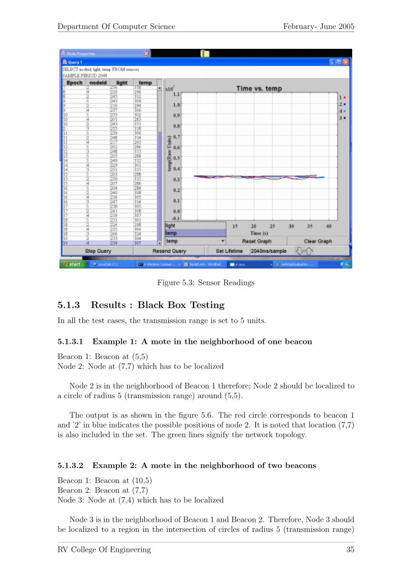
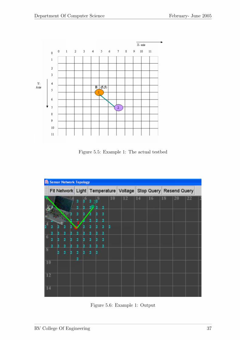
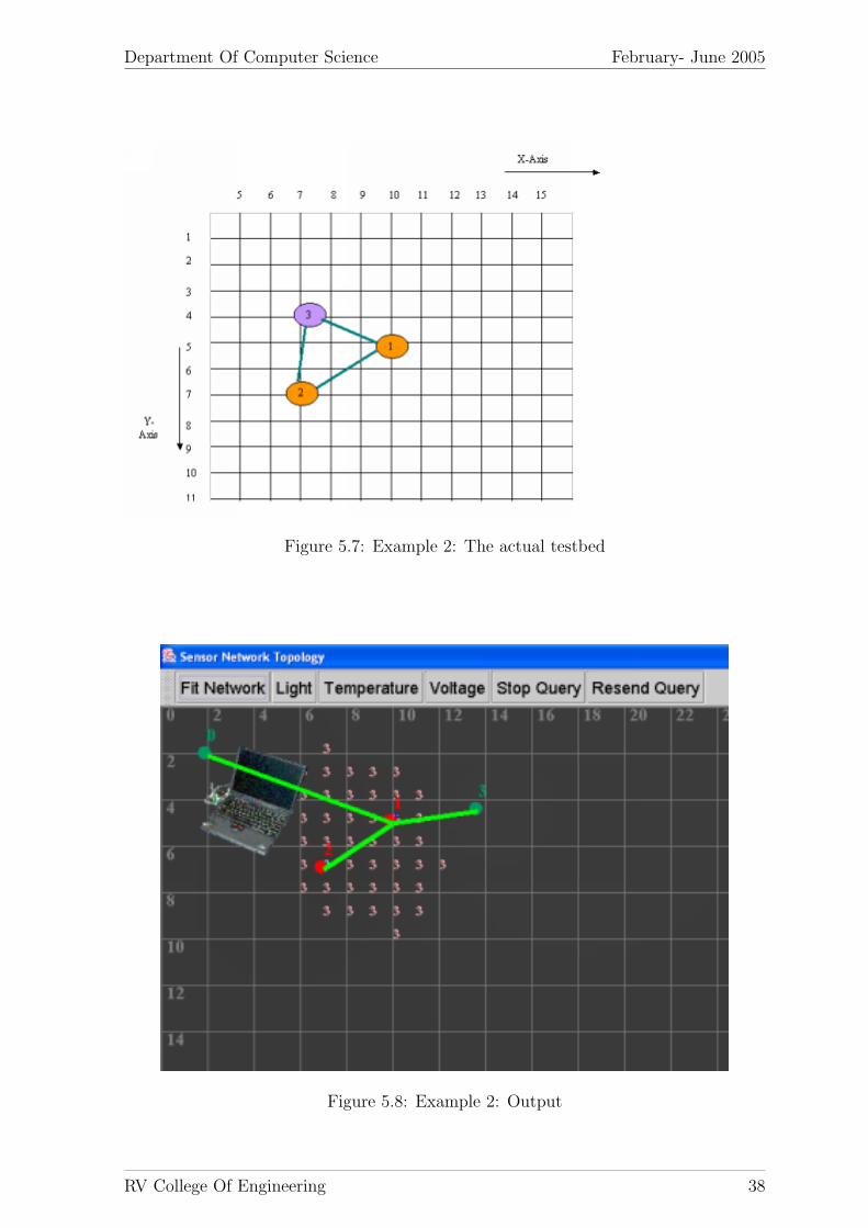
5.1.3.1 Example 1: A mote in the neighborhood of one beacon 355.1.3.2 Example 2: A mote in the neighborhood of two beacons 355.1.3.3 Example 3: A mote in the neighbourhood of one beacon

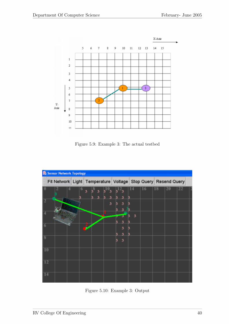
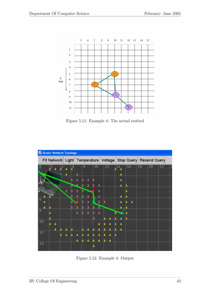
but not the other . . . . . . . . . . . . . . . . . . . . . 395.1.3.4 Example 4: A mote in the neighbourhood of no beacons 41

6 Conclusion 43

7 Limitations and Future Enhancement 44

A nesC Files : Detection of Neighbors 45A.1 Query for Neighbors . . . . . . . . . . . . . . . . . . . . . . . . . . . . 45

A.1.1 SendQueryC.nc . . . . . . . . . . . . . . . . . . . . . . . . . . . 45A.1.1.1 SendQueryM.nc . . . . . . . . . . . . . . . . . . . . . . 45

A.2 Respond to Request/Neighbor Information . . . . . . . . . . . . . . . . 46A.2.1 Receiver.h . . . . . . . . . . . . . . . . . . . . . . . . . . . . . . 46A.2.2 ReceiverC.nc . . . . . . . . . . . . . . . . . . . . . . . . . . . . 47A.2.3 ReceiverM.nc . . . . . . . . . . . . . . . . . . . . . . . . . . . . 47

B Java File : Localization.java 52

RV College Of Engineering iii


List of Figures

2.1 A typical sensor network . . . . . . . . . . . . . . . . . . . . . . . . . . 22.2 Beacon Mote and Localization . . . . . . . . . . . . . . . . . . . . . . . 10

3.1 Crossbow’s mica2 mote and sensor . . . . . . . . . . . . . . . . . . . . 13

4.1 0-Level DFD . . . . . . . . . . . . . . . . . . . . . . . . . . . . . . . . . 264.2 1-Level DFD . . . . . . . . . . . . . . . . . . . . . . . . . . . . . . . . . 274.3 Localization with IR . . . . . . . . . . . . . . . . . . . . . . . . . . . . 27

5.1 TinyDB GUI . . . . . . . . . . . . . . . . . . . . . . . . . . . . . . . . 335.2 Modified frontend to encorporate localization. . . . . . . . . . . . . . . 345.3 Sensor Readings . . . . . . . . . . . . . . . . . . . . . . . . . . . . . . . 355.4 Localization: A multihop scenario . . . . . . . . . . . . . . . . . . . . . 365.5 Example 1: The actual testbed . . . . . . . . . . . . . . . . . . . . . . 375.6 Example 1: Output . . . . . . . . . . . . . . . . . . . . . . . . . . . . . 375.7 Example 2: The actual testbed . . . . . . . . . . . . . . . . . . . . . . 385.8 Example 2: Output . . . . . . . . . . . . . . . . . . . . . . . . . . . . . 385.9 Example 3: The actual testbed . . . . . . . . . . . . . . . . . . . . . . 405.10 Example 3: Output . . . . . . . . . . . . . . . . . . . . . . . . . . . . . 405.11 Example 4: The actual testbed . . . . . . . . . . . . . . . . . . . . . . 425.12 Example 4: Output . . . . . . . . . . . . . . . . . . . . . . . . . . . . . 42

RV College Of Engineering iv


Chapter 1

Synopsis

Localization is a fundamental task in wireless ad-hoc networks. We consider the prob-lem of locating and orienting a network of unattended sensor nodes that have beendeployed in a scene at unknown locations. In a location related system, the aqui-sition of objects’ locations is the critical step for the effective and smooth workingprocedures.The basic concept is to deploy a large number of low-cost, self-poweredsensor nodes that acquire and process data. The sensor nodes may include one or moreacoustic microphones as well as seismic, magnetic, or imaging sensors. A typical sensornetwork objective is to detect, track, and classify objects or events in the neighborhoodof the network.

We consider location estimation in networks where a small proportion of devices,called reference devices or beacons, have a priori information about their coordinates.All devices,regardless of their absolute coordinate knowledge, estimate the range be-tween themselves and their neighboring devices. Such location estimation is called rel-ative location because the range estimates collected are predominantly between pairsof devices of which neither has absolute coordinate knowledge.We intend to implement a simple method of localization called the in-range methodIR to a two-dimensional network of sensor nodes. The basic premise of IR is that thetransmission at a given power can be decoded only upto a maximum distance calledits transmission range. Therefore, if a node is able to receive a signal from a beacon,this would imply that the node can be localized to a set of positions represented by adisc of radius equal to the transmission range. Similarly a localized node would be ableto aid the localization of its other neighbours. In this way, an iterative process couldbe used, by which the sensors can collaboratively learn and improve their localizationregions .Nodes use this simple connectivity metric, to infer proximity to a given subset of thesereference points. Nodes localize themselves to their proximate reference points. Theaccuracy of localization is then dependent on the separation distance between twoadjacent reference points and the transmission range of these reference points.

RV College Of Engineering 1


Chapter 2

Introduction

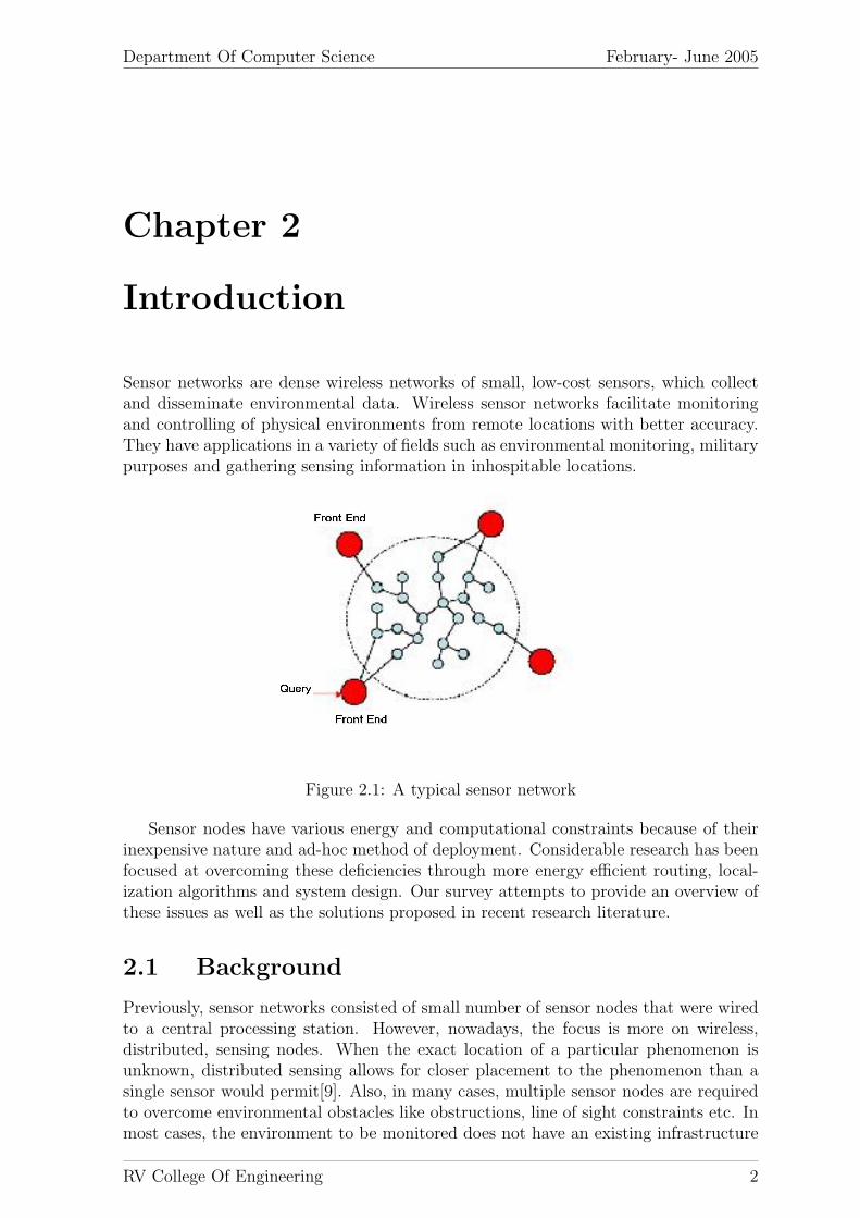
Sensor networks are dense wireless networks of small, low-cost sensors, which collectand disseminate environmental data. Wireless sensor networks facilitate monitoringand controlling of physical environments from remote locations with better accuracy.They have applications in a variety of fields such as environmental monitoring, militarypurposes and gathering sensing information in inhospitable locations.

Figure 2.1: A typical sensor network

Sensor nodes have various energy and computational constraints because of theirinexpensive nature and ad-hoc method of deployment. Considerable research has beenfocused at overcoming these deficiencies through more energy efficient routing, local-ization algorithms and system design. Our survey attempts to provide an overview ofthese issues as well as the solutions proposed in recent research literature.

2.1 Background

Previously, sensor networks consisted of small number of sensor nodes that were wiredto a central processing station. However, nowadays, the focus is more on wireless,distributed, sensing nodes. When the exact location of a particular phenomenon isunknown, distributed sensing allows for closer placement to the phenomenon than asingle sensor would permit[9]. Also, in many cases, multiple sensor nodes are requiredto overcome environmental obstacles like obstructions, line of sight constraints etc. Inmost cases, the environment to be monitored does not have an existing infrastructure



for either energy or communication. It becomes imperative for sensor nodes to surviveon small, finite sources of energy and communicate through a wireless communicationchannel. Another requirement for sensor networks would be distributed processingcapability. This is necessary since communication is a major consumer of energy. Acentralized system would mean that some of the sensors would need to communicateover long distances that lead to even more energy depletion. Hence, it would be a goodidea to process locally as much information as possible in order to minimize the totalnumber of bits transmitted.

2.1.1 Sensor Sub-systems

A sensor node usually consists of four sub-systems[10]:

2.1.1.1 A computing subsystem

It consists of a microprocessor(micro controller unit, MCU), which is responsible for thecontrol of the sensors and execution of communication protocols. MCUs usually operateunder various operating modes for power management purposes. But shuttling betweenthese operating modes involves consumption of power, so the energy consumption levelsof the various modes should be considered while looking at the battery lifetime of eachnode.

2.1.1.2 A communication subsystem

It consists of a short-range radio, which is used to communicate with neighboring nodesand the outside world. Radios can operate under the Transmit, Receive, Idle and Sleepmodes. It is important to completely shut down the radio rather than put it in the idlemode when it is not transmitting or receiving because of the high power consumed inthis mode.

2.1.1.3 A sensing subsystem

It consists of a group of sensors and actuators and links the node to the outside world.Using low power components and saving power at the cost of performance, which isnot required, can reduce energy consumption.

2.1.1.4 A power supply subsystem

It consists of a battery, which supplies power to the node. It should be seen that theamount of power drawn from a battery is checked because if high current is drawnfrom a battery for a long time, the battery will die even though it could have goneon for a longer time. Usually the rated current capacity of a battery being used fora sensor node is lesser than the minimum energy consumption required leading to thelower battery lifetimes. Reducing the current drastically or even turning it off oftencan increase the lifetime of a battery.

2.1.2 Challenges

In spite of the diverse applications, sensor networks pose a number of unique technicalchallenges due to the following factors:



• Ad hoc deployment: Most sensor nodes are deployed in regions, which haveno infrastructure at all. A typical way of deployment in a forest would be tossingthe sensor nodes from an aeroplane. In such a situation, it is up to the nodes toidentify its connectivity and distribution.

• Unattended operation: In most cases, once deployed, sensor networks haveno human intervention. Hence the nodes themselves are responsible for reconfig-uration in case of any changes.

• Untethered: The sensor nodes are not connected to any energy source. Thereis only a finite source of energy, which must be optimally used for processingand communication. An interesting fact is that communication dominates pro-cessing in energy consumption. Thus, in order to make optimal use of energy,communication should be minimized as much as possible.

• Dynamic changes: It is required that a sensor network system be adaptable tochanging connectivity (for e.g., due to addition of more nodes, failure of nodesetc.) as well as changing environmental stimuli.

Thus, unlike traditional networks, where the focus is on maximizing channel throughputor minimizing node deployment, the major consideration in a sensor network is toextend the system lifetime as well as the system robustness [8].

2.1.3 Important aspects

2.1.3.1 Localization

In most of the cases, sensor nodes are deployed in an ad hoc manner. It is up tothe nodes to identify themselves in some spatial co-ordinate system. This problem isreferred to as localization. This aspect is discussed later.

2.1.3.2 Energy Efficiency

Energy consumption is the most important factor to determine the life of a sensornetwork because usually sensor nodes are driven by battery and have very low energyresources. This makes energy optimization more complicated in sensor networks be-cause it involved not only reduction of energy consumption but also prolonging the lifeof the network as much as possible. Having energy awareness in every aspect of designand operation can do this. This ensures that energy awareness is also incorporatedinto groups of communicating sensor nodes and the entire network and not only in theindividual nodes.Developing design methodologies and architectures, which help in energy aware designof sensor networks, can reduce the power consumed by the sensor nodes. The lifetime ofa sensor network can be increased significantly if the operating system, the applicationlayer and the network protocols are designed to be energy aware. Power managementin radios is very important because radio communication consumes a lot of energyduring operation of the system. Another aspect of sensor nodes is that a sensor nodealso acts a router and a majority of the packets, which the sensor receives, are meantto be forwarded. Intelligent radio hardware that help in identifying and redirectingpackets which need to be forwarded and in the process reduce the computing overheadbecause the packets are no longer processed in the intermediate nodes.



Traffic can also be distributed in such a way as to maximize the life of the network.A path should not be used continuously to forward packets regardless of how muchenergy is saved because this depletes the energy of the nodes on this path and there isa breach in the connectivity of the network. It is better that the load of the traffic bedistributed more uniformly throughout the network. It is important that the users beupdated on the health of a sensor network because this would serve as a warning of afailure and aid in the deployment of additional sensors.

2.1.3.3 Routing

Conventional routing protocols have several limitations when being used in sensornetworks due to the energy-constrained nature of these networks. These protocolsessentially follow the flooding technique in which a node stores the data item it receivesand then sends copies of the data item to all its neighbors.

• Implosion: If a node is a common neighbor to nodes holding the same data item,then it will get multiple copies of the same data item. Therefore, the protocolwastes resources sending the data item and receiving it.

• Resource management: In conventional flooding, nodes are not resource-aware. They continue with their activities regardless of the energy availableto them at a given time.

The routing protocols designed for sensor networks should be able to overcome boththese deficiencies or/and look at newer ways of conserving energy increasing the lifeof the network in the process. Ad-hoc routing protocols are also unsuitable for sensornetworks because they try to eliminate the high cost of table updates when there ishighly mobility of nodes in the network. But unlike ad-hoc networks, sensor networksare not highly mobile. Routing protocols can be divided into proactive and reactiveprotocols. Proactive protocols attempt at maintaining consistent updated routing in-formation between all the nodes by maintaining one or more routing tables. In reactiveprotocols, the routes are only created when they are needed. The routing can be eithersource-initiated or destination-initiated.

2.1.3.4 Media Access Control in Sensor Networks

Media Access Control in sensor networks is very different than in the traditional net-works because of its constraints on computational ability, storage and energy resources.Therefore media access control should be energy efficient and should also allocate band-width fairly to the infrastructure of all nodes in the network. In sensor networks, theprimary objective is to sample the residing environment for information and send it toa higher processing infrastructure (base station) after processing it. The data trafficmay be low for lengthy periods with intense traffic in between for short periods of time.Most of the time, the traffic is multihop and heading towards some larger processinginfrastructure. At each of the nodes, there is traffic originating out of the node andtraffic being routed through the node because most nodes are both data sources androuters. There are several limitations on sensor nodes too. They have little or no ded-icated carrier sensing or collision detection and they have no specific protocol stacks,which could specify the design of their media access protocol.

• Fairness

The following are the challenges in multihop sensor networks



– The originating traffic from a node has to compete with the traffic beingrouted through that node.

– An undetected node might exist in the network, which might result in un-expected contention for bandwidth with route-thru traffic.

– The probability of corruption and contention at every hop is higher for thenodes, which reside farther away from the higher processing infrastructure.

– Energy is invested in every packet when it is routed through every node.Therefore, the longer a packet has been routed, the more expensive it is todrop that packet.

Listening to the network, which is expensive, can do carrier sensing in sensornetworks. Therefore the listening period should be short to conserve energy.The traffic also tends to be highly synchronized because nearby nodes tend tosend messages to report the same event. Since there is no collision detection,the nodes will tend to corrupt each other’s messages when they send them atthe same time. This could happen every time they detect a common event. Toreduce contentions, a back off mechanism could be used. A node could restrainitself from transmitting for a certain period of time and hopefully the channelbecomes clear after the back off period. This will help in desynchronizing thetraffic too. Contention protocols in traditional networks widely use the Requestto Send(RTS), Clear to Send(CTS) and acknowledgements(ACK) to reduce con-tentions. A RTS-CTS-DATA-ACK handshake is extremely costly though whenused in sensor networks because every message transmitted uses up the low en-ergy resources of the nodes. Therefore, the number of control packets used shouldbe kept as low as possible. Thus, only the RTS and CTS messages are used inthe control scheme. If a node does not receive the CTS after sending the RTSfor a long time, the node will back off for a binary exponentially increasing timeperiod and then transmit again. If it receives a CTS, which is not meant forit or receives a CTS before its own transmission, it will back off to avoid colli-sions. Fairness in allocation between the originating traffic and route-thru trafficshould be achieved. The media access controls the originating traffic when theroute-thru traffic is high and when the originating traffic is high, it applies abackpressure to control the route-thru traffic deep down in the network fromwhere it originated. A linear increase and multiplicative decrease approach isused for transmission control. The transmission rate control is probabilistic andit is linearly increased by a constant and it is decreased by multiplying it with, a,where a is less than 1 and greater than 0. Since dropping traffic which is beingrouted through is wastage of the network’s energy resources, more preference isgiven to it by making its dropping penalty 50

The advantage of this scheme is that the amount of computation required for thisis within the sensor nodes’ computational capability and achieves good energyefficiency when the traffic is low while maintaining the fairness among the nodes.

• S-MAC .The major sources of energy wastage are:

– Collisions

– Overhearing

– Control packet overhead



– Idle listening

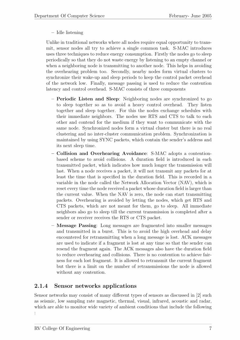
Unlike in traditional networks where all nodes require equal opportunity to trans-mit, sensor nodes all try to achieve a single common task. S-MAC introducesuses three techniques to reduce energy consumption. Firstly the nodes go to sleepperiodically so that they do not waste energy by listening to an empty channel orwhen a neighboring node is transmitting to another node. This helps in avoidingthe overhearing problem too. Secondly, nearby nodes form virtual clusters tosynchronize their wake-up and sleep periods to keep the control packet overheadof the network low. Finally, message passing is used to reduce the contentionlatency and control overhead. S-MAC consists of three components

– Periodic Listen and Sleep: Neighboring nodes are synchronized to goto sleep together so as to avoid a heavy control overhead. They listentogether and sleep together. For this the nodes exchange schedules withtheir immediate neighbors. The nodes use RTS and CTS to talk to eachother and contend for the medium if they want to communicate with thesame node. Synchronized nodes form a virtual cluster but there is no realclustering and no inter-cluster communication problem. Synchronization ismaintained by using SYNC packets, which contain the sender’s address andits next sleep time.

– Collision and Overhearing Avoidance: S-MAC adopts a contention-based scheme to avoid collisions. A duration field is introduced in eachtransmitted packet, which indicates how much longer the transmission willlast. When a node receives a packet, it will not transmit any packets for atleast the time that is specified in the duration field. This is recorded in avariable in the node called the Network Allocation Vector (NAV), which isreset every time the node received a packet whose duration field is larger thanthe current value. When the NAV is zero, the node can start transmittingpackets. Overhearing is avoided by letting the nodes, which get RTS andCTS packets, which are not meant for them, go to sleep. All immediateneighbors also go to sleep till the current transmission is completed after asender or receiver receives the RTS or CTS packet.

– Message Passing: Long messages are fragmented into smaller messagesand transmitted in a burst. This is to avoid the high overhead and delayencountered for retransmitting when a long message is lost. ACK messagesare used to indicate if a fragment is lost at any time so that the sender canresend the fragment again. The ACK messages also have the duration fieldto reduce overhearing and collisions. There is no contention to achieve fair-ness for each lost fragment. It is allowed to retransmit the current fragmentbut there is a limit on the number of retransmissions the node is allowedwithout any contention.

2.1.4 Sensor networks applications

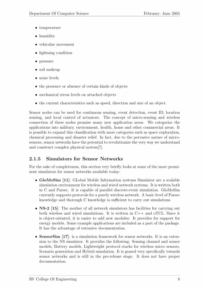
Sensor networks may consist of many different types of sensors as discussed in [2] suchas seismic, low sampling rate magnetic, thermal, visual, infrared, acoustic and radar,which are able to monitor wide variety of ambient conditions that include the following:



• temperature

• humidity

• vehicular movement

• lightning condition

• pressure

• soil makeup

• noise levels

• the presence or absence of certain kinds of objects

• mechanical stress levels on attached objects

• the current characteristics such as speed, direction and size of an object.

Sensor nodes can be used for continuous sensing, event detection, event ID, locationsensing, and local control of actuators. The concept of micro-sensing and wirelessconnection of these nodes promise many new application areas. We categorize theapplications into military, environment, health, home and other commercial areas. Itis possible to expand this classification with more categories such as space exploration,chemical processing and disaster relief. In fact, due to the pervasive nature of micro-sensors, sensor networks have the potential to revolutionize the very way we understandand construct complex physical system[7].

2.1.5 Simulators for Sensor Networks

For the sake of completeness, this section very briefly looks at some of the more promi-nent simulators for sensor networks available today:

• GloMoSim [11]: GLobal Mobile Information systems Simulator are a scalablesimulation environment for wireless and wired network systems. It is written bothin C and Parsec. It is capable of parallel discrete-event simulation. GloMoSimcurrently supports protocols for a purely wireless network. A basic level of Parsecknowledge and thorough C knowledge is sufficient to carry out simulations

• NS-2 [15]: The mother of all network simulators has facilities for carrying outboth wireless and wired simulations. It is written in C++ and oTCL. Since itis object-oriented, it is easier to add new modules. It provides for support forenergy models. Some example applications are included as a part of the package.It has the advantage of extensive documentation.

• SensorSim [17]: is a simulation framework for sensor networks. It is an exten-sion to the NS simulator. It provides the following: Sensing channel and sensormodels, Battery models, Lightweight protocol stacks for wireless micro sensors,Scenario generation and Hybrid simulation. It is geared very specifically towardssensor networks and is still in the pre-release stage. It does not have properdocumentation.



2.2 Localization

In sensor networks, nodes are deployed into an unplanned infrastructure where thereis no a priori knowledge of location. The problem of estimating spatial-coordinatesof the node is referred to as localization. An immediate solution, which comes tomind, is GPS or the Global Positioning System. The different approaches to thelocalization problem have been studied in [3, 4, 5]. However, there are some strongfactors against the usage of GPS. For one, GPS can work only outdoors. Secondly,GPS receivers are expensive and not suitable in the construction of small cheap sensornodes. A third factor is that it cannot work in the presence of any obstruction likedense foliage etc. Thus, sensor nodes would need to have other means of establishingtheir positions and organizing themselves into a co-ordinate system without relyingon an existing infrastructure. Most of the proposed localization techniques today,depend on recursive trilateration/multilateration techniques[8]. One way of consideringsensor networks is taking the network to be organized as a hierarchy with the nodesin the upper level being more complex and already knowing their location throughsome technique (say, through GPS). These nodes then act as beacons by transmittingtheir position periodically. The nodes, which have not yet inferred their position,listen to broadcasts from these beacons and use the information from beacons with lowmessage loss to calculate its own position. A simple technique would be to calculateits position as the centroid of all the locations it has obtained. This is called asproximity based localization. It is quite possible that all nodes do not have accessto the beacons. In this case, the nodes, which have obtained their position throughproximity, based localization themselves act as beacons to the other nodes. This processis called iterative multilateration. As can be guessed, iterative multilateration leads toaccumulation of localization error. Thus, trilateration is a geometric principle whichallows us to find a location if its distance from three already-known locations. Thesame principle is extended to three-dimensional space. In this case, spheres insteadof circles are used and four spheres would be needed. When a localization techniqueusing beacons is used, an important question would be ’how many initial beacons todeploy. Too many beacons would result in self-interference among the beacons whiletoo less number of beacons would mean that many of the nodes would have to dependon iterative multilateration.

2.2.1 Localization Techniques

Localization can be classified as fine-grained, which refers to the methods based ontiming/signal strength and coarse-grained, which refers to the techniques based onproximity to a reference point. [6] gives an over-view of the various localization tech-niques. Examples of fine-grained localization are:

• Timing: The distance between the receiver node and a reference point is deter-mined by the time of flight of the communication signal.

• Signal strength: As a signal propagates, attenuation takes place proportionalto the distance traveled. This fact is made use of to calculate the distance.

• Signal pattern matching: In this method, the coverage area is pre-scannedwith transmitting signals. A central system assigns a unique signature for eachsquare in the location grid. The system matches a transmitting signal from amobile transmitter with the pre-constructed database and arrives at the correct



location. But pre-generating the database goes against the idea of ad hoc de-ployment.

• Directionality: Here, the angle of each reference point with respect to themobile node in some reference frame is used to determine the location.

Examples of coarse-grained localization is proximity based localization as describedearlier. [6] proposes a localization system which is RF-based, receiver-based, ad hoc,responsive, low-energy consuming and adaptive. RF-based transceivers would be moreinexpensive and smaller compared to GPS-receivers. Also in an infrastructure lessenvironment, the deployment would be ad hoc and the nodes should be able to adaptthemselves to available reference points.

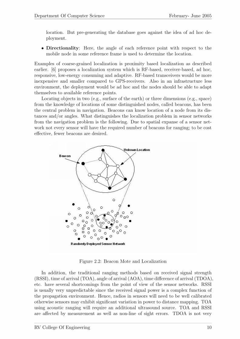
Locating objects in two (e.g., surface of the earth) or three dimensions (e.g., space)from the knowledge of locations of some distinguished nodes, called beacons, has beenthe central problem in navigation. Beacons can know location of a node from its dis-tances and/or angles. What distinguishes the localization problem in sensor networksfrom the navigation problem is the following. Due to spatial expanse of a sensor net-work not every sensor will have the required number of beacons for ranging; to be costeffective, fewer beacons are desired.

Figure 2.2: Beacon Mote and Localization

In addition, the traditional ranging methods based on received signal strength(RSSI), time of arrival (TOA), angle of arrival (AOA), time difference of arrival (TDOA),etc. have several shortcomings from the point of view of the sensor networks. RSSIis usually very unpredictable since the received signal power is a complex function ofthe propagation environment. Hence, radios in sensors will need to be well calibratedotherwise sensors may exhibit significant variation in power to distance mapping. TOAusing acoustic ranging will require an additional ultrasound source. TOA and RSSIare affected by measurement as well as non-line of sight errors. TDOA is not very



practical for a distributed implementation. AOA sensing will require either an antennaarray or several ultra-sound receivers. This motivates us to consider a particularly sim-ple method of localization as in [1], which we call the in-range method (IR). Here weimplement a simple method of localization in sensor networks in which a sensor withunknown location is localized to a disk of radius equal to the transmission range cen-tered at a beacon if the sensor under consideration can receive a transmission from thebeacon. This is a reliable and extremely easy-to-implement technique since it assumesonly a basic communication capability. The real advantage, however, is that once local-ized, a sensor aids the other sensors in localization. This way by collaboration sensorscan learn and improve their localization regions iteratively. We analyze this iterativescheme and construct a distributed algorithm for utilizing it in real sensor networks.The basic premise of IR is that a transmission at a given power can be decoded only upto a maximum distance, called its transmission range. IR then simply localizes a nodewith unknown location to a disk of radius equal to the range centered at a beacon ifthe node under consideration can successfully decode a transmission from the beacon..



Chapter 3

System Requirement Specification

3.1 Hardware specifications

The hardware required is as follows:

• Motes (having a processor with small memory)

• Sensors (to be attached to the motes, to detect temperature, light etc).

• Antennas (for wireless communication between the motes)

• Base Station (attached to the serial port of the PC/Laptop)

• PC/Laptop (to collect the readings from the motes and display the readingsand positions)

3.1.1 Crossbow Mica mote and sensors

Crossbows [16] wireless sensor platform gives the flexibility to create powerful, tether-less, and automated data collection and monitoring systems. Crossbows supports awide range of hardware and sensors for various customer requirements. Most of thehardware can plug-and-play and it all runs TinyOS / nesC from UC Berkeley. Theplatform consists of Processor Radio boards (MPR) commonly referred to as MOTES.These battery powered devices run TinyOS and support two-way mesh radio networks.Sensor and data acquisition cards (MTS and MDA) plug into the Mote Processor Radioboards. Sensor support includes both direct sensing as well interfaces for externalsensors. Finally, gateway and interface products (MIB), allow customers to interfaceMotes to PCs, PDAs, the WWW, and existing wired networks and protocols. TheTinyOS operating system is open-source, extendable, and scalable. Code modulesare wired together allowing fluent-C programmers to custom design systems quickly.Accessory products include antennae, cables, and packaging.

Specifications of Mica mote are as follows:

• Processor: Atmel ATmega 128L

• Frequency Range: 902 to 928 MHz - 433.1 to 434.8 MHz

• Nonvolatile Memory: 512 KB Since these motes have a small memory, runningcomplex calculations on them is not possible.

• Attached AA Battery Pack



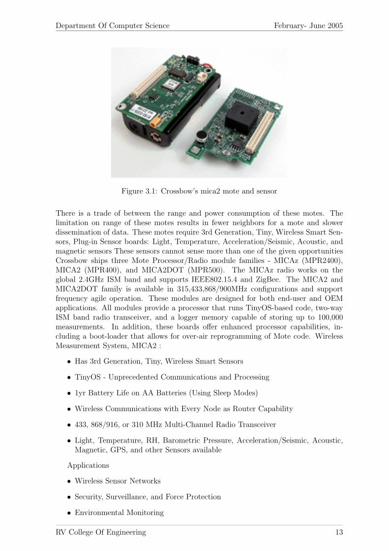
Figure 3.1: Crossbow’s mica2 mote and sensor

There is a trade of between the range and power consumption of these motes. Thelimitation on range of these motes results in fewer neighbors for a mote and slowerdissemination of data. These motes require 3rd Generation, Tiny, Wireless Smart Sen-sors, Plug-in Sensor boards: Light, Temperature, Acceleration/Seismic, Acoustic, andmagnetic sensors These sensors cannot sense more than one of the given opportunitiesCrossbow ships three Mote Processor/Radio module families - MICAz (MPR2400),MICA2 (MPR400), and MICA2DOT (MPR500). The MICAz radio works on theglobal 2.4GHz ISM band and supports IEEE802.15.4 and ZigBee. The MICA2 andMICA2DOT family is available in 315,433,868/900MHz configurations and supportfrequency agile operation. These modules are designed for both end-user and OEMapplications. All modules provide a processor that runs TinyOS-based code, two-wayISM band radio transceiver, and a logger memory capable of storing up to 100,000measurements. In addition, these boards offer enhanced processor capabilities, in-cluding a boot-loader that allows for over-air reprogramming of Mote code. WirelessMeasurement System, MICA2 :

• Has 3rd Generation, Tiny, Wireless Smart Sensors

• TinyOS - Unprecedented Communications and Processing

• 1yr Battery Life on AA Batteries (Using Sleep Modes)

• Wireless Communications with Every Node as Router Capability

• 433, 868/916, or 310 MHz Multi-Channel Radio Transceiver

• Light, Temperature, RH, Barometric Pressure, Acceleration/Seismic, Acoustic,Magnetic, GPS, and other Sensors available

Applications

• Wireless Sensor Networks

• Security, Surveillance, and Force Protection

• Environmental Monitoring



• Large Scale Wireless Networks

• Distributed Computing Platform

3.2 Software Specifications

• TinyOS and NesC: TinyOSis an open source operating system designed forwireless sensor networks that supports Crossbow Mica motes, Mica2 motes andMica2Dot motes and a few other wireless sensor devices. TinyOS is embeddedin Crossbow motes and therefore we will use TinyOS structures for developingthe system. Programming language used to develop software on TinyOS is nesC.nesC is an extension to C that involves the necessary structures and concepts tosupport event-driven execution of TinyOS and this project will be implementedusing nesC programming language.

• TinyDB: TinyDB which is query processing system for extracting informationfrom a network of TinyOS sensors In addition to the mote software, TinyDBprovides a PC interface written in Java. JDK 1.3 or later is required. TheTinyDB software is to be modified to encoorporate the localization algorithm.

• Java: The packet information retrieval, localization algorithm and frontend dis-play along with the topology and the locations is coded in java.

3.2.1 TinyOS

It [14] is an open-source operating system designed for wireless embedded sensor net-works. It features a component-based architecture which enables rapid innovation andimplementation while minimizing code size as required by the severe memory con-straints inherent in sensor networks. TinyOS’s component library includes networkprotocols, distributed services, sensor drivers, and data acquisition tools - all of whichcan be used as-is or be further refined for a custom application. TinyOS’s event-drivenexecution model enables fine-grained power management yet allows the schedulingflexibility made necessary by the unpredictable nature of wireless communication andphysical world interfaces. TinyOS has been ported to over a dozen platforms and nu-merous sensor boards. A wide community uses it in simulation to develop and testvarious algorithms and protocols. New releases see over 10,000 downloads. Over 500research groups and companies are using TinyOS on the Berkeley/Crossbow Motes.Numerous groups are actively contributing code to the sourceforge site and workingtogether to establish standard, interoperable network services built from a base of directexperience and honed through competitive analysis in an open environment.

3.2.1.1 TinyOS Application

Some final comments about a TinyOS application are due and their implications. Sinceeverything in a TinyOS application is static:

• No Dynamic Memory (no malloc)

• No Function Pointers

• No Heap



This means that just about everything is known at compile time by the nesC compiler.This allows the compiler to perform global compile time analysis to detect data raceconditions, and where function inlining will improve performance. This relieves thedeveloper of these burdens and hence development is made easier and the systemsrobustness is improved. The memory map of a TinyOS application is similar to thestructure of an executable image on the Unix OS. The Harvard architecture of a COTSMote (i.e. the Atmel MCU) partitions the memory into two segments: the staticprogram flash memory and the dynamic data SRAM. Each segment has it’s own bus.The advantage of this architecture is it allows data and executable code to be fetchedin parallel and allows many instructions to executed in one CPU cycle. The Mica2generation of COTS Motes ( our case ) consists of 128k of program flash and 4k ofSRAM. The memory image is as follows: In the 128K Program Flash

• ”text” section - Executable Code

• ”data” section - Program Constants

In the 4K SRAM

• ”bss” section - Variables

• The rest of the bss is free space - fixed (no dynamic memory)

• stack - grows down in the free space

3.2.2 nesC

nesC [13](pronounced “NES-see”) is an extension to the C programming languagedesigned to embody the structuring concepts and execution model of TinyOS .TinyOSis an event-driven operating system designed for sensor network nodes that have verylimited resources (e.g., 8K bytes of program memory, 512 bytes of RAM). The basicconcepts behind nesC are:

• Separation of construction and composition: programs are built out of compo-nents, which are assembled (”wired”) to form whole programs. Components haveinternal concurrency in the form of tasks. Threads of control may pass into acomponent through its interfaces. These threads are rooted either in a task or ahardware interrupt.

• Specification of component behaviour in terms of set of interfaces: Interfaces maybe provided or used by components. The provided interfaces are intended torepresent the functionality that the component provides to its user, the usedinterfaces represent the functionality the component needs to perform its job.

• Interfaces are bidirectional: they specify a set of functions to be implementedby the interface’s provider (commands) and a set to be implemented by the in-terface’s user (events). This allows a single interface to represent a complexinteraction between components (e.g., registration of interest in some event, fol-lowed by a callback when that event happens). This is critical because all lengthycommands in TinyOS (e.g. send packet) are non-blocking; their completion issignaled through an event (send done). By specifying interfaces, a componentcannot call the send command unless it provides an implementation of the send-Done event.



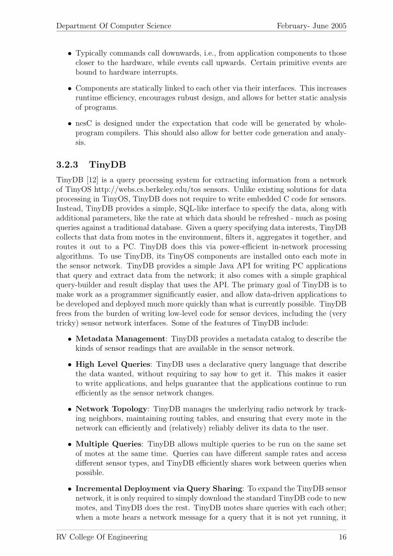
• Typically commands call downwards, i.e., from application components to thosecloser to the hardware, while events call upwards. Certain primitive events arebound to hardware interrupts.

• Components are statically linked to each other via their interfaces. This increasesruntime efficiency, encourages rubust design, and allows for better static analysisof programs.

• nesC is designed under the expectation that code will be generated by whole-program compilers. This should also allow for better code generation and analy-sis.

3.2.3 TinyDB

TinyDB [12] is a query processing system for extracting information from a networkof TinyOS http://webs.cs.berkeley.edu/tos sensors. Unlike existing solutions for dataprocessing in TinyOS, TinyDB does not require to write embedded C code for sensors.Instead, TinyDB provides a simple, SQL-like interface to specify the data, along withadditional parameters, like the rate at which data should be refreshed - much as posingqueries against a traditional database. Given a query specifying data interests, TinyDBcollects that data from motes in the environment, filters it, aggregates it together, androutes it out to a PC. TinyDB does this via power-efficient in-network processingalgorithms. To use TinyDB, its TinyOS components are installed onto each mote inthe sensor network. TinyDB provides a simple Java API for writing PC applicationsthat query and extract data from the network; it also comes with a simple graphicalquery-builder and result display that uses the API. The primary goal of TinyDB is tomake work as a programmer significantly easier, and allow data-driven applications tobe developed and deployed much more quickly than what is currently possible. TinyDBfrees from the burden of writing low-level code for sensor devices, including the (verytricky) sensor network interfaces. Some of the features of TinyDB include:

• Metadata Management: TinyDB provides a metadata catalog to describe thekinds of sensor readings that are available in the sensor network.

• High Level Queries: TinyDB uses a declarative query language that describethe data wanted, without requiring to say how to get it. This makes it easierto write applications, and helps guarantee that the applications continue to runefficiently as the sensor network changes.

• Network Topology: TinyDB manages the underlying radio network by track-ing neighbors, maintaining routing tables, and ensuring that every mote in thenetwork can efficiently and (relatively) reliably deliver its data to the user.

• Multiple Queries: TinyDB allows multiple queries to be run on the same setof motes at the same time. Queries can have different sample rates and accessdifferent sensor types, and TinyDB efficiently shares work between queries whenpossible.

• Incremental Deployment via Query Sharing: To expand the TinyDB sensornetwork, it is only required to simply download the standard TinyDB code to newmotes, and TinyDB does the rest. TinyDB motes share queries with each other;when a mote hears a network message for a query that it is not yet running, it



automatically asks the sender of that data for a copy of the query, and beginsrunning it. No programming or configuration of the new motes is required beyondinstalling TinyDB.

3.2.3.1 System Overview

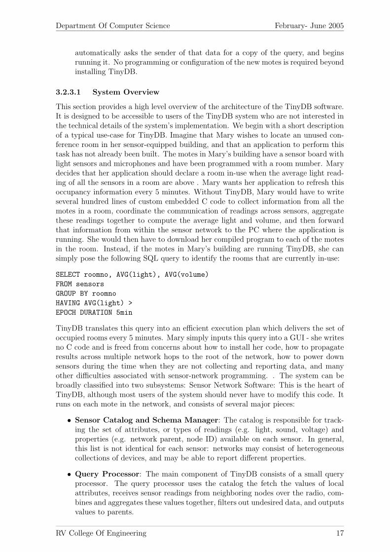
This section provides a high level overview of the architecture of the TinyDB software.It is designed to be accessible to users of the TinyDB system who are not interested inthe technical details of the system’s implementation. We begin with a short descriptionof a typical use-case for TinyDB. Imagine that Mary wishes to locate an unused con-ference room in her sensor-equipped building, and that an application to perform thistask has not already been built. The motes in Mary’s building have a sensor board withlight sensors and microphones and have been programmed with a room number. Marydecides that her application should declare a room in-use when the average light read-ing of all the sensors in a room are above . Mary wants her application to refresh thisoccupancy information every 5 minutes. Without TinyDB, Mary would have to writeseveral hundred lines of custom embedded C code to collect information from all themotes in a room, coordinate the communication of readings across sensors, aggregatethese readings together to compute the average light and volume, and then forwardthat information from within the sensor network to the PC where the application isrunning. She would then have to download her compiled program to each of the motesin the room. Instead, if the motes in Mary’s building are running TinyDB, she cansimply pose the following SQL query to identify the rooms that are currently in-use:

SELECT roomno, AVG(light), AVG(volume)

FROM sensors

GROUP BY roomno

HAVING AVG(light) >

EPOCH DURATION 5min

TinyDB translates this query into an efficient execution plan which delivers the set ofoccupied rooms every 5 minutes. Mary simply inputs this query into a GUI - she writesno C code and is freed from concerns about how to install her code, how to propagateresults across multiple network hops to the root of the network, how to power downsensors during the time when they are not collecting and reporting data, and manyother difficulties associated with sensor-network programming. . The system can bebroadly classified into two subsystems: Sensor Network Software: This is the heart ofTinyDB, although most users of the system should never have to modify this code. Itruns on each mote in the network, and consists of several major pieces:

• Sensor Catalog and Schema Manager: The catalog is responsible for track-ing the set of attributes, or types of readings (e.g. light, sound, voltage) andproperties (e.g. network parent, node ID) available on each sensor. In general,this list is not identical for each sensor: networks may consist of heterogeneouscollections of devices, and may be able to report different properties.

• Query Processor: The main component of TinyDB consists of a small queryprocessor. The query processor uses the catalog the fetch the values of localattributes, receives sensor readings from neighboring nodes over the radio, com-bines and aggregates these values together, filters out undesired data, and outputsvalues to parents.



• Memory Manager: TinyDB extends TinyOS with a small, handle-based dy-namic memory manager

• Network Topology Manager: TinyDB manages the connectivity of motes inthe network, to efficiently route data and query sub-results through the network.

• Java-based Client Interface: A network of TinyDB motes is accessed froma connected PC through the TinyDB client interface, which consists of a setof Java classes and applications. These classes are all stored in the tinyos-1.x/tools/java/tinyos/tinydb package in the source tree.

Major classes include:

• A network interface class that allows applications to inject queries and listen forresults

• Classes to build and transmit queries

• A class to receive and parse query results

• A class to extract information about the attributes and capabilities of devices

• A GUI to construct queries

• A graph and table GUI to display individual sensor results

• A GUI to visualize dynamic network topologies

• An application that uses queries as an interface on top of a network of sensors

3.2.3.2 Installation and Requirements

TinyDB requires a basic TinyOS installation, with a working Java installation (andjavax.comm library). It is currently designed to work with the nesC compiler (nextgeneration C-like language for TinyOS) and avr-gcc 3.3.The most recent version ofTinyDB is always available from the TinyOS SourceForge repository.

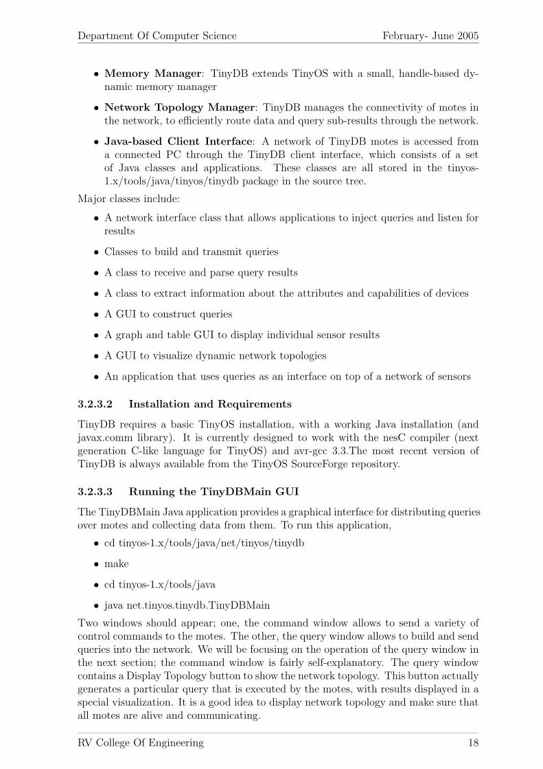
3.2.3.3 Running the TinyDBMain GUI

The TinyDBMain Java application provides a graphical interface for distributing queriesover motes and collecting data from them. To run this application,

• cd tinyos-1.x/tools/java/net/tinyos/tinydb

• make

• cd tinyos-1.x/tools/java

• java net.tinyos.tinydb.TinyDBMain

Two windows should appear; one, the command window allows to send a variety ofcontrol commands to the motes. The other, the query window allows to build and sendqueries into the network. We will be focusing on the operation of the query window inthe next section; the command window is fairly self-explanatory. The query windowcontains a Display Topology button to show the network topology. This button actuallygenerates a particular query that is executed by the motes, with results displayed in aspecial visualization. It is a good idea to display network topology and make sure thatall motes are alive and communicating.



3.2.3.4 Using TinyDB

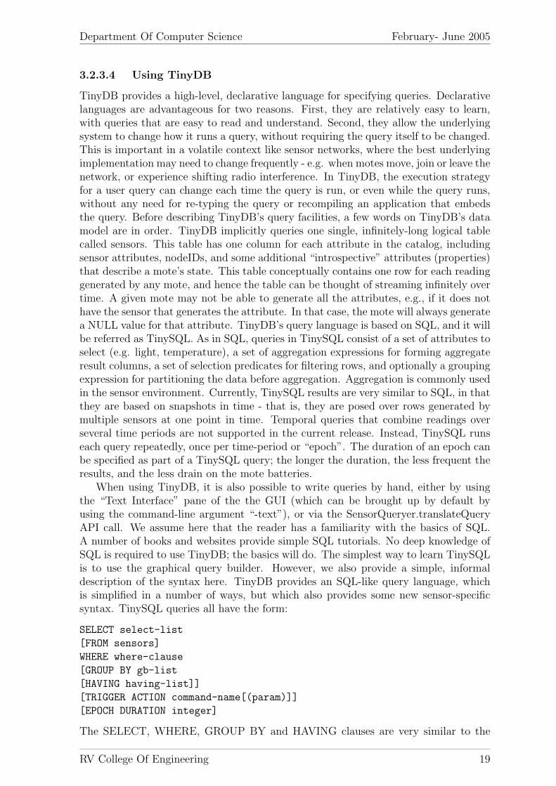
TinyDB provides a high-level, declarative language for specifying queries. Declarativelanguages are advantageous for two reasons. First, they are relatively easy to learn,with queries that are easy to read and understand. Second, they allow the underlyingsystem to change how it runs a query, without requiring the query itself to be changed.This is important in a volatile context like sensor networks, where the best underlyingimplementation may need to change frequently - e.g. when motes move, join or leave thenetwork, or experience shifting radio interference. In TinyDB, the execution strategyfor a user query can change each time the query is run, or even while the query runs,without any need for re-typing the query or recompiling an application that embedsthe query. Before describing TinyDB’s query facilities, a few words on TinyDB’s datamodel are in order. TinyDB implicitly queries one single, infinitely-long logical tablecalled sensors. This table has one column for each attribute in the catalog, includingsensor attributes, nodeIDs, and some additional “introspective” attributes (properties)that describe a mote’s state. This table conceptually contains one row for each readinggenerated by any mote, and hence the table can be thought of streaming infinitely overtime. A given mote may not be able to generate all the attributes, e.g., if it does nothave the sensor that generates the attribute. In that case, the mote will always generatea NULL value for that attribute. TinyDB’s query language is based on SQL, and it willbe referred as TinySQL. As in SQL, queries in TinySQL consist of a set of attributes toselect (e.g. light, temperature), a set of aggregation expressions for forming aggregateresult columns, a set of selection predicates for filtering rows, and optionally a groupingexpression for partitioning the data before aggregation. Aggregation is commonly usedin the sensor environment. Currently, TinySQL results are very similar to SQL, in thatthey are based on snapshots in time - that is, they are posed over rows generated bymultiple sensors at one point in time. Temporal queries that combine readings overseveral time periods are not supported in the current release. Instead, TinySQL runseach query repeatedly, once per time-period or “epoch”. The duration of an epoch canbe specified as part of a TinySQL query; the longer the duration, the less frequent theresults, and the less drain on the mote batteries.

When using TinyDB, it is also possible to write queries by hand, either by usingthe “Text Interface” pane of the the GUI (which can be brought up by default byusing the command-line argument “-text”), or via the SensorQueryer.translateQueryAPI call. We assume here that the reader has a familiarity with the basics of SQL.A number of books and websites provide simple SQL tutorials. No deep knowledge ofSQL is required to use TinyDB; the basics will do. The simplest way to learn TinySQLis to use the graphical query builder. However, we also provide a simple, informaldescription of the syntax here. TinyDB provides an SQL-like query language, whichis simplified in a number of ways, but which also provides some new sensor-specificsyntax. TinySQL queries all have the form:

SELECT select-list

[FROM sensors]

WHERE where-clause

[GROUP BY gb-list

[HAVING having-list]]

[TRIGGER ACTION command-name[(param)]]

[EPOCH DURATION integer]

The SELECT, WHERE, GROUP BY and HAVING clauses are very similar to the



functionality of SQL. Arithmetic expressions are supported in each of these clauses.As in standard SQL, the GROUP BY clause is optional, and if GROUP BY is includedthe HAVING clause may also be used optionally.

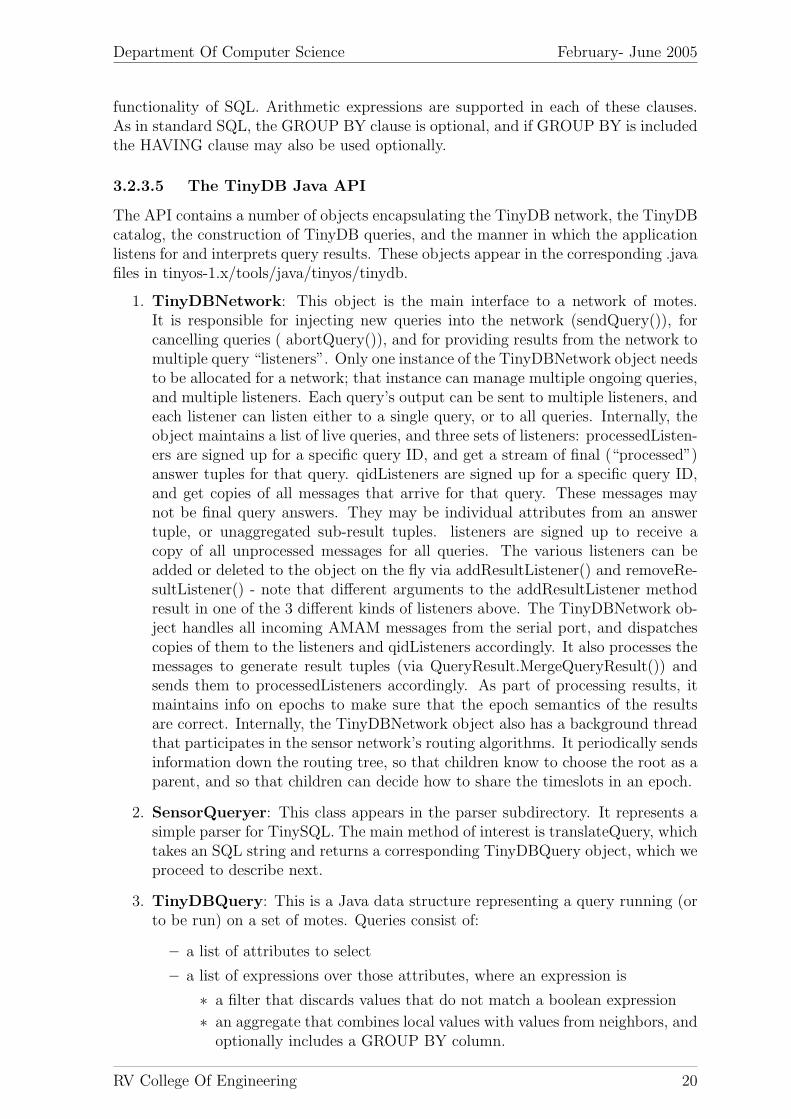
3.2.3.5 The TinyDB Java API

The API contains a number of objects encapsulating the TinyDB network, the TinyDBcatalog, the construction of TinyDB queries, and the manner in which the applicationlistens for and interprets query results. These objects appear in the corresponding .javafiles in tinyos-1.x/tools/java/tinyos/tinydb.

1. TinyDBNetwork: This object is the main interface to a network of motes.It is responsible for injecting new queries into the network (sendQuery()), forcancelling queries ( abortQuery()), and for providing results from the network tomultiple query “listeners”. Only one instance of the TinyDBNetwork object needsto be allocated for a network; that instance can manage multiple ongoing queries,and multiple listeners. Each query’s output can be sent to multiple listeners, andeach listener can listen either to a single query, or to all queries. Internally, theobject maintains a list of live queries, and three sets of listeners: processedListen-ers are signed up for a specific query ID, and get a stream of final (“processed”)answer tuples for that query. qidListeners are signed up for a specific query ID,and get copies of all messages that arrive for that query. These messages maynot be final query answers. They may be individual attributes from an answertuple, or unaggregated sub-result tuples. listeners are signed up to receive acopy of all unprocessed messages for all queries. The various listeners can beadded or deleted to the object on the fly via addResultListener() and removeRe-sultListener() - note that different arguments to the addResultListener methodresult in one of the 3 different kinds of listeners above. The TinyDBNetwork ob-ject handles all incoming AMAM messages from the serial port, and dispatchescopies of them to the listeners and qidListeners accordingly. It also processes themessages to generate result tuples (via QueryResult.MergeQueryResult()) andsends them to processedListeners accordingly. As part of processing results, itmaintains info on epochs to make sure that the epoch semantics of the resultsare correct. Internally, the TinyDBNetwork object also has a background threadthat participates in the sensor network’s routing algorithms. It periodically sendsinformation down the routing tree, so that children know to choose the root as aparent, and so that children can decide how to share the timeslots in an epoch.

2. SensorQueryer: This class appears in the parser subdirectory. It represents asimple parser for TinySQL. The main method of interest is translateQuery, whichtakes an SQL string and returns a corresponding TinyDBQuery object, which weproceed to describe next.

3. TinyDBQuery: This is a Java data structure representing a query running (orto be run) on a set of motes. Queries consist of:

– a list of attributes to select

– a list of expressions over those attributes, where an expression is

∗ a filter that discards values that do not match a boolean expression

∗ an aggregate that combines local values with values from neighbors, andoptionally includes a GROUP BY column.



– an SQL string that should correspond to the expressions listed above.

In addition to allowing a query to be built, this class includes handy methods togenerate specific radio messages for the query, which TinyDBNetwork can use todistribute the query over the network, or to abort the query. It also includes asupport routine for printing the query result schema.

4. QueryResult: This object accepts a query result in the form of an array ofbytes read off the network, parses the results based on a query specification, andprovides a number of utility routines to read the values back. It also providesthe mergeQueryResult functionality for processedListeners. This does concate-nation of multiple aggs as separate attributes of a single result tuple, and finalizesaggregates, by combining data from multiple sensors.

5. AggOp: This provides the code for the aggregation operators SUM, MIN, MAX,and AVG. It includes representation issues (internal network codes for the variousops, and code for pretty-printing), and also the logic for performing final mergesfor each aggregate as part of QueryResult:MergeQueryResult().

6. SelOp: This provides the logic for selection predicates. Currently this includesrepresentations for simple arithmetic comparisons (internal network codes for thearithmetic comparators, and pretty-printing.)

7. Catalog: This object provides a very simple parser for a catalog file - it readsin the file, and after parsing it provides a list of attributes.

8. CommandMsgs: This is a class with static functions to generate message arraysthat can be used to invoke commands on TinyDB motes.

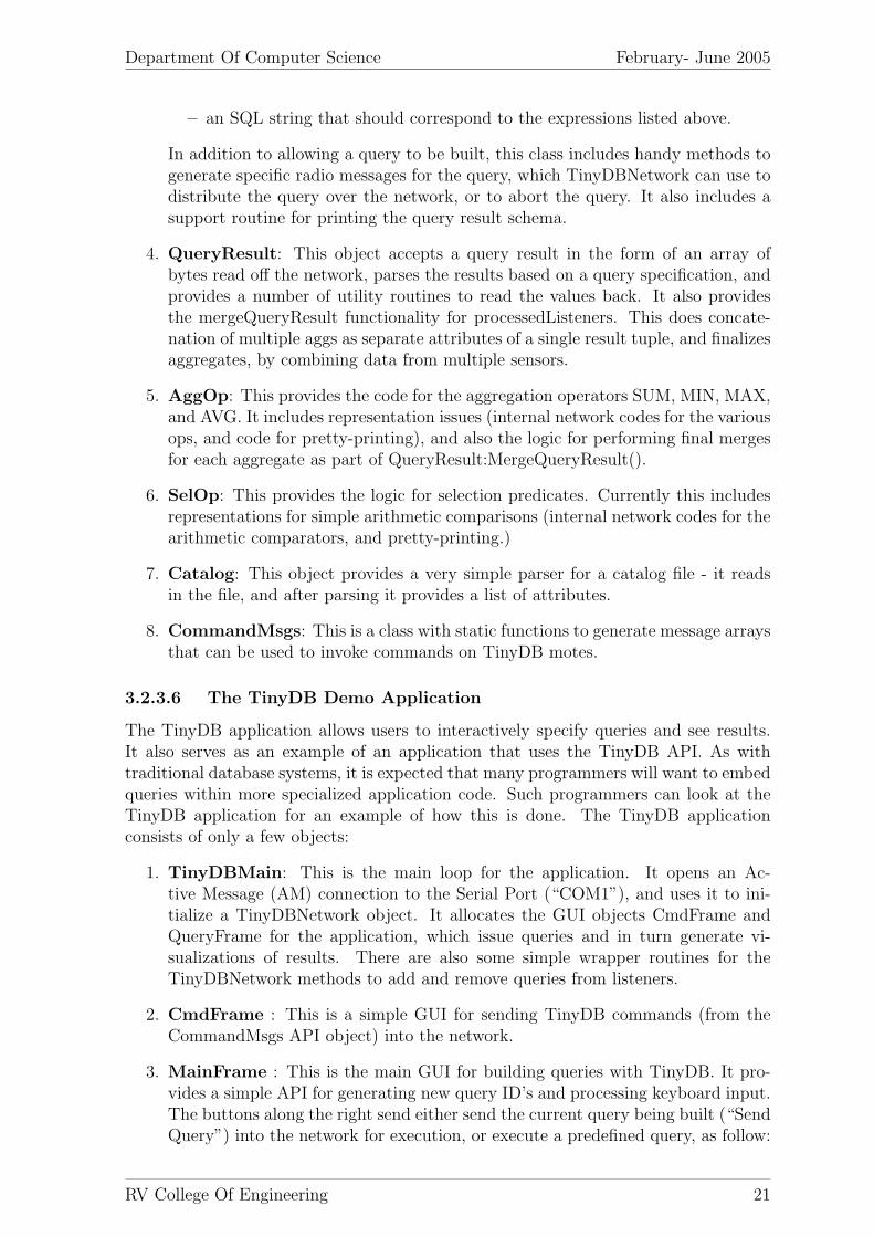
3.2.3.6 The TinyDB Demo Application

The TinyDB application allows users to interactively specify queries and see results.It also serves as an example of an application that uses the TinyDB API. As withtraditional database systems, it is expected that many programmers will want to embedqueries within more specialized application code. Such programmers can look at theTinyDB application for an example of how this is done. The TinyDB applicationconsists of only a few objects:

1. TinyDBMain: This is the main loop for the application. It opens an Ac-tive Message (AM) connection to the Serial Port (“COM1”), and uses it to ini-tialize a TinyDBNetwork object. It allocates the GUI objects CmdFrame andQueryFrame for the application, which issue queries and in turn generate vi-sualizations of results. There are also some simple wrapper routines for theTinyDBNetwork methods to add and remove queries from listeners.

2. CmdFrame : This is a simple GUI for sending TinyDB commands (from theCommandMsgs API object) into the network.

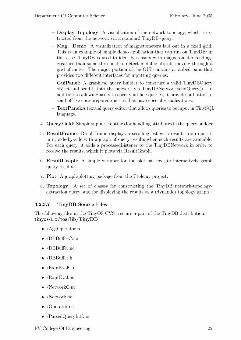
3. MainFrame : This is the main GUI for building queries with TinyDB. It pro-vides a simple API for generating new query ID’s and processing keyboard input.The buttons along the right send either send the current query being built (“SendQuery”) into the network for execution, or execute a predefined query, as follow:



– Display Topology: A visualization of the network topology, which is ex-tracted from the network via a standard TinyDB query.

– Mag. Demo: A visualization of magnetometers laid out in a fixed grid.This is an example of simple demo application that can run on TinyDB: inthis case, TinyDB is used to identify sensors with magnetometer readingsgreather than some threshold to detect metallic objects moving through agrid of motes. The major portion of the GUI contains a tabbed pane thatprovides two different interfaces for inputting queries:

– GuiPanel: A graphical query builder to construct a valid TinyDBQueryobject and send it into the network via TinyDBNetwork.sendQuery() , Inaddition to allowing users to specify ad hoc queries, it provides a button tosend off two pre-prepared queries that have special visualizations:

– TextPanel:A textual query editor that allows queries to be input in TinySQLlanguage.

4. QueryField: Simple support routines for handling attributes in the query builder.

5. ResultFrame: ResultFrame displays a scrolling list with results from queriesin it, side-by-side with a graph of query results when such results are available.For each query, it adds a processedListener to the TinyDBNetwork in order toreceive the results, which it plots via ResultGraph.

6. ResultGraph: A simple wrapper for the plot package, to interactively graphquery results.

7. Plot: A graph-plotting package from the Ptolemy project.

8. Topology: A set of classes for constructing the TinyDB network-topology-extraction query, and for displaying the results as a (dynamic) topology graph.

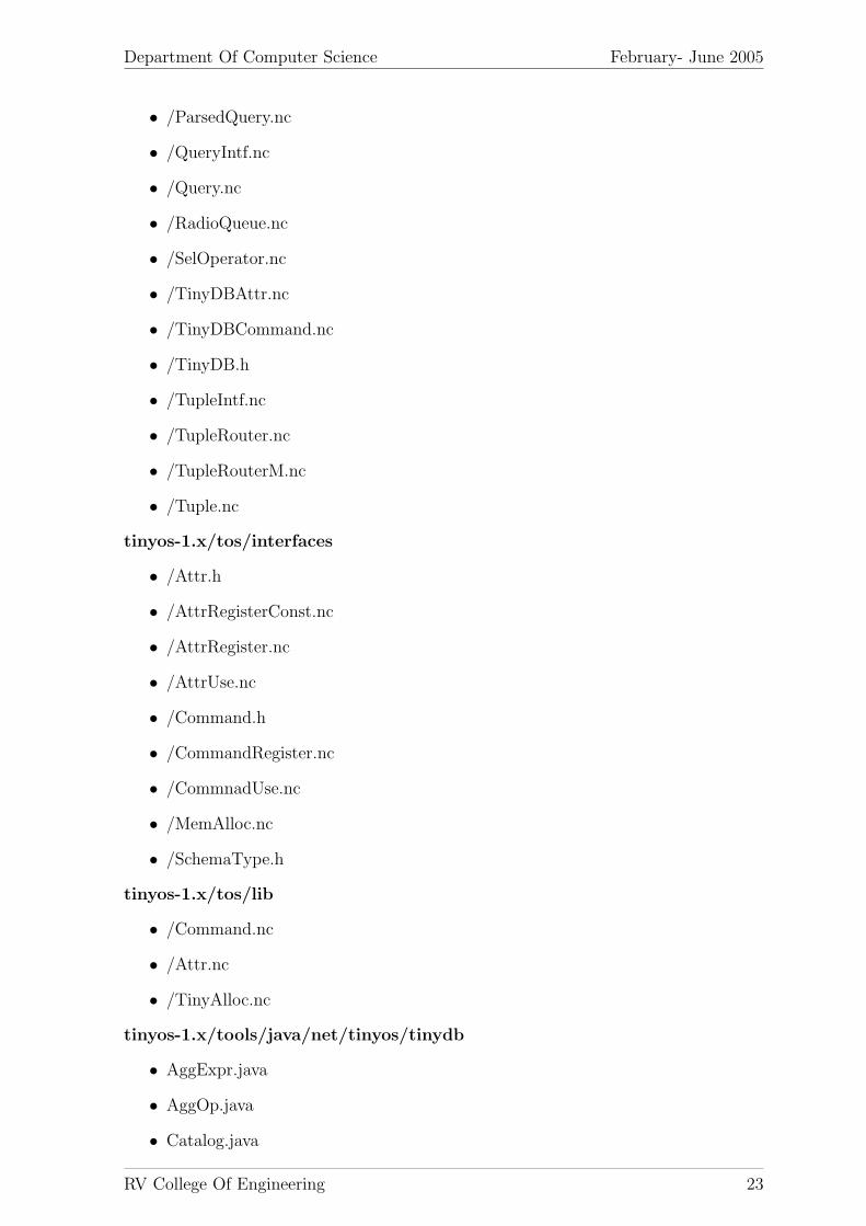
3.2.3.7 TinyDB Source Files

The following files in the TinyOS CVS tree are a part of the TinyDB distribution:tinyos-1.x/tos/lib/TinyDB

• /AggOperator.rd

• /DBBufferC.nc

• /DBBuffer.nc

• /DBBuffer.h

• /ExprEvalC.nc

• /ExprEval.nc

• /NetworkC.nc

• /Network.nc

• /Operator.nc

• /ParsedQueryIntf.nc



• /ParsedQuery.nc

• /QueryIntf.nc

• /Query.nc

• /RadioQueue.nc

• /SelOperator.nc

• /TinyDBAttr.nc

• /TinyDBCommand.nc

• /TinyDB.h

• /TupleIntf.nc

• /TupleRouter.nc

• /TupleRouterM.nc

• /Tuple.nc

tinyos-1.x/tos/interfaces

• /Attr.h

• /AttrRegisterConst.nc

• /AttrRegister.nc

• /AttrUse.nc

• /Command.h

• /CommandRegister.nc

• /CommnadUse.nc

• /MemAlloc.nc

• /SchemaType.h

tinyos-1.x/tos/lib

• /Command.nc

• /Attr.nc

• /TinyAlloc.nc

tinyos-1.x/tools/java/net/tinyos/tinydb

• AggExpr.java

• AggOp.java

• Catalog.java



• CmdFrame.java

• CommandMsgs.java

• MagnetFrame.java

• QueryExpr.java

• QueryField.java

• QueryListener.java

• QueryResult.java

• ResultFrame.java

• ResultGraph.java

• ResultListener.java

• SelExpr.java

• SelOp.java

• TinyDBCmd.java

• TinyDBMain.java

• TinyDBNetwork.java

• TinyDBQuery.java

Makefile

• parser/

– Makefile

– senseParser.cup,lex

• tinyos-1.x/apps/TinyDBApp

– Makefile

– TinyDBApp.nc

3.3 Functional Requirements

The system should be able to

• Fix the positions of the desired beacon motes

• Obtain the neighbours of each sensor in the network

• Based on the knowledge of the positions of beacons and identification of neigh-bours, calculate all possible positions of each sensor in the network i.e localizetheir positions to a fixed set.

• In case of a dynamic system where positions vary constantly, the new locationsof each sensor should also be calculated within a fixed period of time.



3.3.1 Non Functional Requirements

3.3.2 Scalability

Wireless sensor networks generally contain hundreds or even thousands of individualnodes. It is a challenge to show the required performance in functioning of the systemunder such dense networks.

3.3.3 Efficient Data Propagation

Wireless sensor network applications are generally monitoring applications. Most ofthese applications require delivery of data in real-time. Therefore, our system shouldbe efficient while ensuring that it is without extended delays and overheads.

3.3.4 Memory Efficiency

Memory available to the sensors is in the order of KBs, some of which is already filledup by OS and other applications. Therefore, applications and application middlewaresshould be very carefully designed to avoid extensive use of available memory



Chapter 4

Design

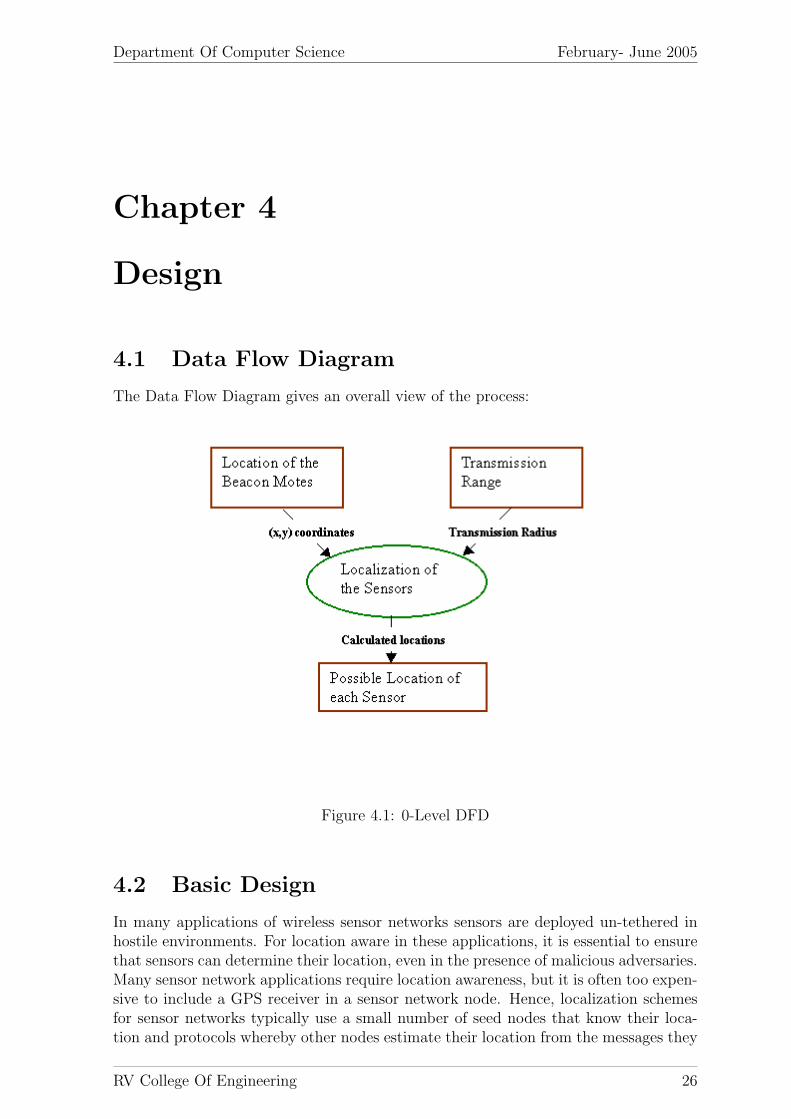
4.1 Data Flow Diagram

The Data Flow Diagram gives an overall view of the process:

Figure 4.1: 0-Level DFD

4.2 Basic Design

In many applications of wireless sensor networks sensors are deployed un-tethered inhostile environments. For location aware in these applications, it is essential to ensurethat sensors can determine their location, even in the presence of malicious adversaries.Many sensor network applications require location awareness, but it is often too expen-sive to include a GPS receiver in a sensor network node. Hence, localization schemesfor sensor networks typically use a small number of seed nodes that know their loca-tion and protocols whereby other nodes estimate their location from the messages they



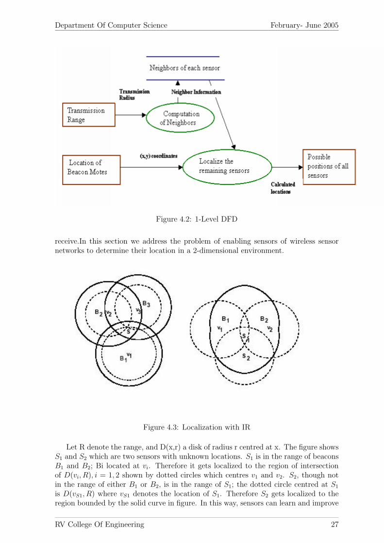
Figure 4.2: 1-Level DFD

receive.In this section we address the problem of enabling sensors of wireless sensornetworks to determine their location in a 2-dimensional environment.

Figure 4.3: Localization with IR

Let R denote the range, and D(x,r) a disk of radius r centred at x. The figure showsS1 and S2 which are two sensors with unknown locations. S1 is in the range of beaconsB1 and B2; Bi located at vi. Therefore it gets localized to the region of intersectionof D(vi, R), i = 1, 2 shown by dotted circles which centres v1 and v2. S2, though notin the range of either B1 or B2, is in the range of S1; the dotted circle centred at S1

is D(vS1, R) where vS1 denotes the location of S1. Therefore S2 gets localized to theregion bounded by the solid curve in figure. In this way, sensors can learn and improve



localization sets iteratively as discussed in [1].

4.3 Algorithm

The algorithm to localize sensors in an ad-hoc network using the in-range method:

1. The positions of beacon motes (the motes whose positions are known) are initial-ized by setting the locX and locY attributes. The entire test bed area is takenas the initial set of positions for the other motes, while the beacon motes haveonly one point in their location set.

2. The neighbors of each sensor are computed as follows:

– Each sensor broadcasts a signal at regular intervals

– The immediate neighbors respond back. The neighbor buffer of the sendersensor is updated each time it receives a response.

– The neighbor information is routed to the main PC via the multi-hop net-work

– The neighbor buffer of each sensor is refreshed periodically (to facilitatedynamic changes)

3. For each sensor, possible locations represented by a set are reckoned by the in-tersection of points in the transmission range of each of its neighbor.

4. If a node is not a neighbor of a sensor, the set of points representing the range ofthe non-neighbor is subtracted from possible locations obtained in step 3. Thisis done because, if a node is a non-neighbor of a sensor, the latter cannot lie inthe range of the former.

5. The intersection of the previous set (calculated in the previous iteration) withthat of possible locations computed from the locations of the neighbors and non-neighbors (from step 4) give the final set of possible locations of the sensor. Thenumber of possible locations of each sensor is non- increasing over iterations.

6. Steps 3 , 4 and 5 are repeated, a chosen number of times till the possible positionsof a sensor is narrowed down to a set of n possibilities, which does not changeover further iterations, or by fixing the number of iterations to a number “n”.



Chapter 5

Testing and Results

When working with embedded devices, it is very difficult to debug applications. Be-cause of this, we have to make sure that the tools that we are using are workingproperly and that the hardware is functioning correctly. This will save countless hoursof searching for bugs in the application when the real problem is in the tools.

5.1 White Box Testing

5.1.1 Unit Testing

Hardware testing involves checking working of the system and the hardware.

5.1.1.1 TinyOS Installation Verification

A TinyOS development environment requires the use of avr gcc compiler, perl, flex,cygwin if you use windows operation system, and JDK 1.3.x or above. TinyOS providesa tool named toscheck to check if the tools have been installed correctly and that theenvironment variables are set.First, we run toscheck (it should be in the current path - a copy is also in tinyos-1.x/tools/scripts). The expected output is as follows:

toscheck

Path:

/usr/local/bin

/usr/bin

/bin

/cygdrive/c/jdk1.3.1_01/bin

/cygdrive/c/WINDOWS/system32

/cygdrive/c/WINDOWS

/cygdrive/c/avrgcc/bin

.

Classpath:

/c/alpha/tools/java:.:/c/jdk1.3.1_01/lib/comm.jar

avrgcc:

/cygdrive/c/avrgcc/bin/avr-gcc

Version: 3.0.2



perl:

/usr/bin/perl

Version: v5.6.1 built for cygwin-multi

flex:

/usr/bin/flex

bison:

/usr/bin/bison

java:

/cygdrive/c/jdk1.3.1_01/bin/java

java version "1.3.1_01"

Java(TM) 2 Runtime Environment, Standard Edition (build 1.3.1_01)

Java HotSpot(TM) Client VM (build 1.3.1_01, mixed mode)

Cygwin:

cygwin1.dll major: 1003

cygwin1.dll minor: 3

cygwin1.dll malloc env: 28

uisp:

/usr/local/bin/uisp

uisp version 20010909

toscheck completed without error.

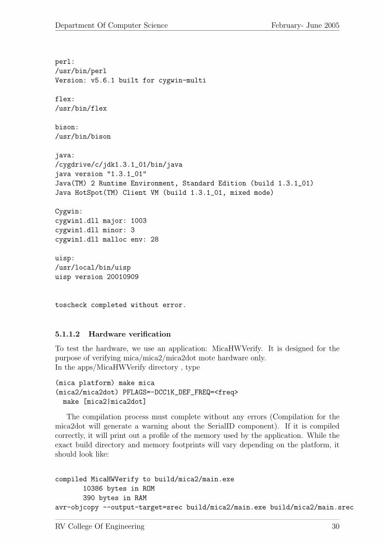
5.1.1.2 Hardware verification

To test the hardware, we use an application: MicaHWVerify. It is designed for thepurpose of verifying mica/mica2/mica2dot mote hardware only.In the apps/MicaHWVerify directory , type

(mica platform) make mica

(mica2/mica2dot) PFLAGS=-DCC1K_DEF_FREQ=<freq>

make [mica2|mica2dot]

The compilation process must complete without any errors (Compilation for themica2dot will generate a warning about the SerialID component). If it is compiledcorrectly, it will print out a profile of the memory used by the application. While theexact build directory and memory footprints will vary depending on the platform, itshould look like:

compiled MicaHWVerify to build/mica2/main.exe

10386 bytes in ROM

390 bytes in RAM

avr-objcopy --output-target=srec build/mica2/main.exe build/mica2/main.srec



Next step is to install the application onto a mote. A powered-on node is placedinto a programming board. The red LED on the programming board should light.The programming board is connected to the parallel port of the computer. To load theprogram on to the device, using a parallel port programmer, we type :

make reinstall [mica|mica2|mica2dot]

The output :

installing mica2 binary

uisp -dprog=<yourprogrammer> -dhost=c62b270 -dpart=ATmega128

--wr_fuse_e=ff --erase --upload if=build/mica2/main.srec

Atmel AVR ATmega128 is found.

Uploading: flash

Fuse Extended Byte set to 0xff

This output shows that the programming tools and the computer’s parallel port areworking.The next step is to verify the mote hardware. First, confirm that the LEDs are blinkinglike a binary counter. Next, the programming board is connected to the serial portof the computer. The hardware verify program will send data over the UART thatcontains it status. To read from the serial port, TinyOS provides a java tool calledhardware check.java. It is located in the same directory. This tool must be builtand run. The commands are shown below assuming COM1 at 57.6 KBaud is used toconnect to the programming board.

make -f jmakefile

MOTECOM=serial@COM1:57600 java hardware_check

The output on the PC is:

hardware_check started

Hardware verification successful.

Node Serial ID: 1 60 48 fb 6 0 0 1d

This program checks the serial ID of the mote (except on the mica2dot), the flashconnectivity, the UART functionality and the external clock. If all status checks arepositive, the hardware verification successful message is printed on the PC screen.If any failure report on the monitor is seen, another mote might be needed.

5.1.1.3 Radio Verification

To verify radio, two nodes are needed . The second node (that has passed the hardwarecheck up to this point) is taken and installed with TOSBase. This node acts as a radiogateway to the first node. Once installed, this node is left in the programming boardand the original node is placed next to it. The hardware check java application is re-run. The output should be the same as shown in the previous section (but will displaythe serial ID of the remote mote). The indication of a working radio system is, again,something like:

hardware_check started

Hardware verification successful.

Node Serial ID: 1 60 48 fb 6 0 0 1d



If the remote mote is turned off or not functioning, it will return a message ”Nodetransmission failure”.If the system and hardware pass all the above tests, TinyOS is ready to be used forbuilding applications.

5.1.1.4 TinyDB Verification

Three motes are required to test the tinydb package. All three are programmed withthe TinyDBApp application, setting their id’s to 0, 1, and 2. The motes are turnedon and are the mote programmed with id 0 is connected to the PC serial port. (Toprogram a mote with a specific id, run make mica install.nodeid, where nodeid is theid with which the mote is associated.)The TinyDBMain class in tools/java/net/tinyos/tinydb is used to interact with themotes The java classes are first built; to do this, we need to ensure that several packagesare in the CLASSPATH. The packages needed are JLex.jar, cup.jar, and plot.jar; allthree are available in tools/java/jars.There is a small program to set your classpath ,called ”javapath” in the tools/java/ directory. To use it, value of the CLASSPATH isset to the output of this command (it will prepend the new directories and jars to yourcurrent CLASSPATH.) To use it under bash (in Cygwin or Linux), we type:

export CLASSPATH=‘path/to/tinyos/tools/java/javapath‘

Under sh or csh ”setenv CLASSPATH ...” is written instead of ”export CLASS-PATH=...”. Now, the java classes are built by typing the following:

cd path/to/tinyos/tools/java/net/tinyos/tinydb

make

This may take several minutes and will output lots of text as the TinyDB query parser iscompiled. Now, the TinyDB GUI is tested by running it from the tools/java directory;

cd ../../..

java net.tinyos.tinydb.TinyDBMain

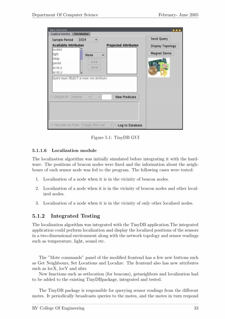
The TinyDB GUI should appear.

The test is complete.

5.1.1.5 GetNeighbours module

The module was loaded in each of the sensors, and the code was tested to ensure thatevery node collects its immediate neigbors accurately. Secondly, the time required toreceive the neighbor information from all the motes was noted. Thirdly, to make surethat the module functions accurately in situations, where nodes change their positionover time, the code was enhanced to encorporate periodic refreshing of the neighborbuffer table. The module was then tested in a dynamic environment.



Figure 5.1: TinyDB GUI

5.1.1.6 Localization module

The localization algorithm was initially simulated before integrating it with the hard-ware. The positions of beacon nodes were fixed and the information about the neigh-bours of each sensor node was fed to the program. The following cases were tested:

1. Localization of a node when it is in the vicinity of beacon nodes.

2. Localization of a node when it is in the vicinity of beacon nodes and other local-ized nodes.

3. Localization of a node when it is in the vicinity of only other localized nodes.

5.1.2 Integrated Testing

The localization algorithm was integrated with the TinyDB application.The integratedapplication could perform localization and display the localized positions of the sensorsin a two-dimensional environment along with the network topology and sensor readingssuch as temperature, light, sound etc.

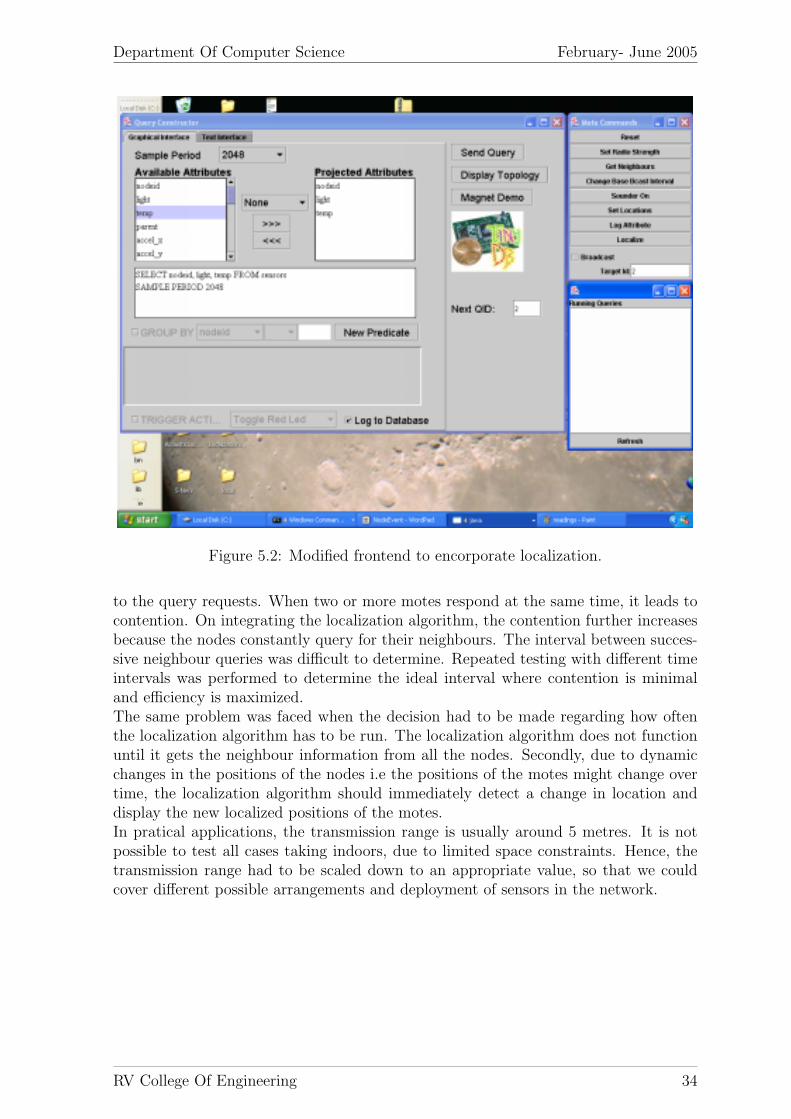
The ”Mote commands” panel of the modified frontend has a few new buttons suchas Get Neighbours, Set Locations and Localize. The frontend also has new attributessuch as locX, locY and nbrs

New functions such as setlocation (for beacons), getneighbors and localization hadto be added to the existing TinyDBpackage, integrated and tested.

The TinyDB package is responsible for querying sensor readings from the differentmotes. It periodically broadcasts queries to the motes, and the motes in turn respond



Figure 5.2: Modified frontend to encorporate localization.

to the query requests. When two or more motes respond at the same time, it leads tocontention. On integrating the localization algorithm, the contention further increasesbecause the nodes constantly query for their neighbours. The interval between succes-sive neighbour queries was difficult to determine. Repeated testing with different timeintervals was performed to determine the ideal interval where contention is minimaland efficiency is maximized.The same problem was faced when the decision had to be made regarding how oftenthe localization algorithm has to be run. The localization algorithm does not functionuntil it gets the neighbour information from all the nodes. Secondly, due to dynamicchanges in the positions of the nodes i.e the positions of the motes might change overtime, the localization algorithm should immediately detect a change in location anddisplay the new localized positions of the motes.In pratical applications, the transmission range is usually around 5 metres. It is notpossible to test all cases taking indoors, due to limited space constraints. Hence, thetransmission range had to be scaled down to an appropriate value, so that we couldcover different possible arrangements and deployment of sensors in the network.



Figure 5.3: Sensor Readings

5.1.3 Results : Black Box Testing

In all the test cases, the transmission range is set to 5 units.

5.1.3.1 Example 1: A mote in the neighborhood of one beacon

Beacon 1: Beacon at (5,5)Node 2: Node at (7,7) which has to be localized

Node 2 is in the neighborhood of Beacon 1 therefore; Node 2 should be localized toa circle of radius 5 (transmission range) around (5,5).

The output is as shown in the figure 5.6. The red circle corresponds to beacon 1and ’2’ in blue indicates the possible positions of node 2. It is noted that location (7,7)is also included in the set. The green lines signify the network topology.

5.1.3.2 Example 2: A mote in the neighborhood of two beacons

Beacon 1: Beacon at (10,5)Beacon 2: Beacon at (7,7)Node 3: Node at (7,4) which has to be localized

Node 3 is in the neighborhood of Beacon 1 and Beacon 2. Therefore, Node 3 shouldbe localized to a region in the intersection of circles of radius 5 (transmission range)



Figure 5.4: Localization: A multihop scenario

around (10,5) and (7,7).The output is as shown in the figure 5.8. The red circles corresponds to beacon 1

and beacon 2. ’3’ in pink indicates the possible positions of node 3. It is noted thatlocation (7,4) is also included in the set. The green lines signify the network topology.



Figure 5.5: Example 1: The actual testbed

Figure 5.6: Example 1: Output







5.1.3.3 Example 3: A mote in the neighbourhood of one beacon but notthe other

Beacon 1: Beacon at (10,5)Beacon 2: Beacon at (7,7)Node 3: Node at (13,5) which has to be localized

Node 3 is in the neighborhood of Beacon 1 but not in the neighborhood of Beacon2. Therefore, Node 3 should be localized to a circle of radius 5 (transmission range)around (10,5) eliminating the points in the circle around (7,7).

The output is as shown in the figure 5.10. The red circles corresponds to beacon 1and beacon 2. ’3’ in pink indicates the possible positions of node 3. It is noted thatlocation (13,5) is also included in the set. The green lines signify the network topology.







5.1.3.4 Example 4: A mote in the neighbourhood of no beacons

Beacon 1: Beacon at (10,5)Beacon 2: Beacon at (7,7)Node 3: Node at (10,9) which has to be localizedNode 4: Node at (12,11) which has to be localized

Node 3 is in the neighborhood of Beacon 1 and in the neighborhood of Beacon 2.Therefore, Node 3 should be localized to the intersections of circles of radius 5 (trans-mission range) with (10,5) and (7,7) as centresNode 4 is only in the neighborhood of Node 3. Therefore Node 4 should be localizedto a set of positions in the neighborhood of the localized positions of Node 3, but aftereliminating the set of points within a circle of radius 5 around (10,5) and (7,7).

The output is as shown in the figure 5.12. The red circles corresponds to beacon 1and beacon 2. ’3’ in pink indicates the possible positions of node 3. It is noted thatlocation (10,9) is also included in the set. ’4’ in yellow indicates the possible positionsof node 4. It is noted that location (12,11) is also included in the set. The green linessignify the network topology.







Chapter 6

Conclusion

Many wireless sensor network applications depend on nodes being able to accuratelydetermine their locations. This is an attempt to study and implement in-range methodof localization in a dynamic environment. This method relies only on the sensorsknowledge of their neighbors and the transmission range. Our main result is thatthe in-range technique can provide accurate localization even when memory limits aresevere, the seed density is low, and network transmissions are highly irregular. Thestrengths of this method lie in its simplicity and efficiency where each sensor localizesitself based on the positions of the beacons and also collaborates with other sensorsaiding their localization. Many issues remain to be explored in future work includinghow well our assumptions hold in different mobile sensor network applications, howdifferent types of motion affect localization, and how our technique can be extended tothe case where RSSI can be used to determine distances between the nodes.



Chapter 7

Limitations and FutureEnhancement

While the in-range method is a simple, non-complex method of finding the positions ofthe sensors, it does not give the accurate position of the sensor. The maximum error inthe position is constrained by the transmission range. The worst-case scenario occurs,when a node is in the vicinity of only a single other node (or beacon), then the possiblelocation of the former node becomes the entire transmission range of the latter.Secondly, it is not possible to fix the transmission range exactly to a certain numberof units. The range oscillates from the fixed value by a small value that can be takento be negligible but it coarsens the results.The range changes from environment to environment, from indoor to outdoor. Thus,fixing the range value for the localization algorithm becomes difficult.The neighbor information from each of the motes is routed to the PC. The localizationalgorithm can function only it obtains all the neighbor information. This latency istotally dependent on the number of nodes. As the number of nodes is increased, thecontention and routing time increases.As the number of nodes increases, the number of iterations in the localization in-rangemethod will also increase. Hence, the IR range method has a complexity proportionalto the number of nodes.

Thus, the next task is to find a more optimized solution to the localization aspectin sensor networks. Finding the approximate distance between the nodes by usingother methods could reduce the error in locations. One example is acoustic rangingmethod, where the distances are reckoned by sending a sound signal and the time ofthe signal. Thus, the possible locations confines to a hollow band (taking toleranceinto consideration) rather than an entire circular area of transmission.Once the positions of the nodes have been discovered, the next task is to place a buzzerin the room. The sensors are to be placed on moving vehicles (toy cars for e.g.), whichperiodically sense the buzzer. Based on the intensity of the buzzer signal and themomentary positions of the sensor, the approximate location of the buzzer has to bedetermined. In this way the localization algorithm could used to track other objectsin the environment



Appendix A

nesC Files : Detection of Neighbors

A.1 Query for Neighbors

A.1.1 SendQueryC.nc

c on f i gu r a t i on CmdReg{

}

implementation {

components Main , GetNeighbhorsC , SingleTimer , CmdRegM, Command;

Main . StdControl −> GetNeighbhorsC . StdControl ;Main . StdControl −> CmdRegM. StdControl ;Main . StdControl −> SingleTimer . StdControl ;CmdRegM.Commands −> Command;CmdRegM. Timer −> SingleTimer . Timer ;

}

A.1.1.1 SendQueryM.nc

#define MAX NODE ID 50module CmdRegM {

prov ide s i n t e r f a c e StdControl ;

uses {

i n t e r f a c e CommandUse as Commands ;i n t e r f a c e Timer ;

}

}

implementation {

command r e s u l t t StdControl . i n i t ( ) {return SUCCESS;

}



command r e s u l t t StdControl . s t a r t ( ) {

return c a l l Timer . s t a r t (TIMER ONE SHOT, 1000 ) ;}

command r e s u l t t StdControl . stop ( ) {

return SUCCESS;

}

event r e s u l t t Timer . f i r e d ( ) {

ParamVals paramVals ;char r e su l tBu f [ 1 0 ] ;SchemaErrorNo errorNo ;stat ic u in t 16 t daddr=1;

/∗ Set Des t ina t ion Address ∗/

paramVals . numParams = 1 ;daddr = TOS BCAST ADDR;paramVals . paramDataPtr [ 0 ] = (char ∗)&daddr ;

i f ( c a l l Commands . invoke ( ”SENDMSG” , re su l tBuf ,&errorNo , &paramVals ) == FAIL)

return FAIL ;

return SUCCESS;

}

event r e s u l t t Commands . commandDone(char ∗commandName ,char ∗ re su l tBuf , SchemaErrorNo errorNo ) {

return SUCCESS;}

}

A.2 Respond to Request/Neighbor Information

A.2.1 Receiver.h

#ifndef GLOBAL#define GLOBALenum {

AM GETNEIGHBHORS = 120} ;enum {

DATA LEN = 2} ;enum {

REQUEST = 1} ;enum {

RESPONSE = 2} ;enum {



MAX NUM OF NEIGHBHORS = 25} ;enum {

REFRESH = 255} ;

typedef struct NeighbhorData {u i n t 8 t saddr ;u i n t 8 t msgType ;

} NeighbhorData ;

typedef struct neighbhors {u i n t 8 t addr ;u i n t 16 t r s s i ;

}neighbhors ;#endif

A.2.2 ReceiverC.nc

i n c l ud e s GetNeighbhors ;

c on f i gu r a t i on GetNeighbhorsC {prov ide s i n t e r f a c e StdControl ;

}

implementation {

StdControl = GetNeighbhorsM . StdControl ;//Main . StdContro l −> GetNeighbhorsM . StdContro l ;GetNeighbhorsM . SendMsg −> Comm. SendMsg [AM GETNEIGHBHORS] ;GetNeighbhorsM . ReceiveMsg −> Comm. ReceiveMsg [AM GETNEIGHBHORS] ;GetNeighbhorsM . Reg i s t e r −> Command.Cmd[ unique ( ”Command” ) ] ;GetNeighbhorsM . Leds −> LedsC ;GetNeighbhorsM . CommControl −> Comm. Control ;GetNeighbhorsM . SetValue −> GlobalM . SetValue ;GetNeighbhorsM . GetValue −> GlobalM . GetValue ;GetNeighbhorsM .Commands −> Command;GetNeighbhorsM .Random −> RandomLFSR;GetNeighbhorsM . SetReqSentFlag −> ReqSentFlagM . SetReqSentFlag ;GetNeighbhorsM . GetReqSentFlag −> ReqSentFlagM . GetReqSentFlag ;GetNeighbhorsM . RadioControl −> CC1000ControlM . CC1000Control ;GetNeighbhorsM . MicroTimer −> MicroTimerM . MicroTimer ;GetNeighbhorsM . RefreshNeighbhorsTable −> GlobalM . StdControl ;

}

A.2.3 ReceiverM.nc

i n c l ud e s GetNeighbhors ;

module GetNeighbhorsM {

prov ide s {

i n t e r f a c e StdControl ;}

uses {i n t e r f a c e CC1000Control as RadioControl ;i n t e r f a c e CommandRegister as Reg i s t e r ;



i n t e r f a c e ReceiveMsg ;i n t e r f a c e SendMsg ;i n t e r f a c e StdControl as CommControl ;i n t e r f a c e Random ;i n t e r f a c e Leds ;i n t e r f a c e GetValue ;i n t e r f a c e SetValue ;i n t e r f a c e CommandUse as Commands ;i n t e r f a c e SetReqSentFlag ;i n t e r f a c e GetReqSentFlag ;i n t e r f a c e MicroTimer ;i n t e r f a c e StdControl as RefreshNeighbhorsTable ;

}}

implementation {

TOS Msg retBuf , respBuf , globalTosMsg ;u i n t 16 t globalDaddr ;TOS MsgPtr pmsg=&retBuf ;NeighbhorData ∗data ;

command r e s u l t t StdControl . i n i t ( ) {

c a l l CommControl . i n i t ( ) ;c a l l Leds . i n i t ( ) ;c a l l Random . i n i t ( ) ;

return SUCCESS;}

command r e s u l t t StdControl . s t a r t ( ) {

ParamList paramList ;

c a l l CommControl . s t a r t ( ) ;

/∗ Set Radio Power ∗/

i f ( c a l l RadioControl . SetRFPower (1 ) == FAIL) {

c a l l Leds . ye l lowToggle ( ) ;}

/∗ Reg i s t e r Command to Send Request ∗/

paramList . params [ 0 ] = UINT16 ;paramList . numParams = 1 ;i f ( c a l l Reg i s t e r . registerCommand ( ”SENDMSG” , VOID, 0 ,

&paramList ) == FAIL) {return FAIL ;

}

/∗ Set Timer ∗/

i f (TOS LOCAL ADDRESS != 0) {

c a l l MicroTimer . s t a r t (5000000) ;}



return SUCCESS;}

command r e s u l t t StdControl . stop ( ) {

c a l l CommControl . s top ( ) ;

return SUCCESS;}

event r e s u l t t Reg i s t e r . commandFunc(char ∗commandName , char ∗ re su l tBuf ,SchemaErrorNo ∗ errorNo , ParamVals ∗params ) {

NeighbhorData ∗PayLoad ;u i n t 8 t loca lNode id =0;

/∗ Get Local node ID ∗/

l o ca lNode id = TOS LOCAL ADDRESS;

/∗ Assign to Globa l v a r i a b l e s ∗/

globalDaddr =∗ ( ( u i n t 16 t ∗) params−>paramDataPtr [ 0 ] ) ;

/∗ F i l l Payload ∗/

memset ( ( char ∗)&globalTosMsg , 0 , s izeof ( globalTosMsg ) ) ;PayLoad = ( NeighbhorData ∗) globalTosMsg . data ;PayLoad−>msgType = REQUEST;PayLoad−>saddr = loca lNode id ;globalTosMsg . l ength = DATA LEN;

/∗ Send Request ∗/

i f ( c a l l SendMsg . send ( globalDaddr , DATA LEN,&globalTosMsg ) == FAIL) {


c a l l SetReqSentFlag . s e t ( 1 ) ;

return SUCCESS;}

event r e s u l t t SendMsg . sendDone (TOS MsgPtr msg , r e s u l t t s u c c e s s ) {

char buf [ 1 0 ] ;SchemaErrorNo errNo ;

c a l l Leds . redToggle ( ) ;

return SUCCESS;}

event TOS MsgPtr ReceiveMsg . r e c e i v e (TOS MsgPtr msg) {



TOS Msg tosMsg ;TOS MsgPtr r e t ;NeighbhorData ∗ resData ;u i n t 8 t loca lNode id ;u i n t 16 t backoffTime ;

/∗ Buf fer swapping ∗/

c a l l Leds . greenToggle ( ) ;

r e t = pmsg ;pmsg = msg ;memset ( ( char ∗)&tosMsg , 0 , s izeof ( tosMsg ) ) ;data = ( NeighbhorData ∗)msg−>data ;

/∗ Process Request ∗/

i f ( data−>msgType == REQUEST) {

/∗ Get Local node ID ∗/

l o ca lNode id = TOS LOCAL ADDRESS;resData = ( NeighbhorData ∗) respBuf . data ;resData−>msgType = RESPONSE;resData−>saddr = loca lNode id ;

/∗ Send Response ∗/

i f (TOS LOCAL ADDRESS == 0) {return r e t ;

}

i f ( c a l l SendMsg . send ( data−>saddr ,DATA LEN, &respBuf ) == FAIL) {


return r e t ;}

i f ( data−>msgType == RESPONSE) {c a l l SetValue . s e t ( data−>saddr , msg−>s t r ength ) ;

}

return r e t ;}

event r e s u l t t Commands . commandDone(char ∗commandName ,char ∗ re su l tBuf , SchemaErrorNo errorNo ) {

return SUCCESS;}

async event r e s u l t t MicroTimer . f i r e d ( ) {

ParamVals paramVals ;char buf [ 1 0 ] ;SchemaErrorNo errNo ;



u in t 16 t daddr ;stat ic u i n t 8 t re f r e shCounte r =0;

/∗ Per iod ic Refresh o f Neighbhors Table once in a Minute ∗/

r e f r e shCounte r++;re f r e shCounte r = 0 ;c a l l RefreshNeighbhorsTable . s t a r t ( ) ;c a l l SetValue . s e t (REFRESH, REFRESH) ;

/∗ Send Request f o r Neighbhors ∗/

daddr = TOS BCAST ADDR;paramVals . numParams = 1 ;paramVals . paramDataPtr [ 0 ] = (char ∗)&daddr ;i f ( c a l l Commands . invoke ( ”SENDMSG” ,buf , &errNo , &paramVals ) == FAIL) {


return SUCCESS;

}

} /∗ End implementat ion ∗/



Appendix B

Java File : Localization.java

%\ begin%verbatim}

/∗ The f o l l ow i n g code c a r r i e s out the l o c a l i z a t i o n on the sensors :The ne ighbours o f the motes are taken as the input to the module and thei t e r a t i v e procedure i s ca r r i e d out p e r i o d i c a l l y ∗/

package net . t i nyo s . t inydb ;import java . i o . ∗ ;import net . t i nyo s . t inydb . g l oba l ;

pub l i c c l a s s l o c a l i z a t i o n{

int noofnodes = 20 ;/∗no . o f nodes i s taken to be 20 ; i t can be changed acco rd ing l y ∗/

pub l i c stat ic boolean array [ ] [ ] [ ] ;/∗ the array v a r i a b l e s i g n i f i e s whether i t i s p o s s i b l e f o r a nodeto be occupied at a p a r t i c u l a r p o s i t i o ni f array [ i ] [ x ] [ y]= t rue => ( x , y ) i s a v i a b l e p o s i t i o n o f node i ;i f array [ i ] [ x ] [ y]= f a l s e => ( x , y ) i s a not a v i a b l e p o s i t i o n o f node i ; ∗/

boolean nbrs [ ] [ ] ;/∗ S im i l a r l y i f nbrs [ i ] [ j ]= t rue =>node i i s a neighbour o f node j ;S im i l a r l y i f nbrs [ i ] [ j ]= f a l s e =>node i i s not a neighbour o f node j ; ∗/

boolean beacon [ ] ;/∗ i f beacon [ i ]= t rue => node i i s a beacon mote ;i f beacon [ i ]= f a l s e => node i i s not a beacon mote ; ∗/}

boolean [ ] [ ]i n t e r s e c t i o n ( boolean arr1 [ ] [ ] , boolean arr2 [ ] [ ] )/∗

c a l c u l a t e s the i n t e r s e c t i o n o f 2 s e t s d e p i c t i n g p o s s i b l e l o c a t i o n s∗/

{boolean r e s u l t [ ] [ ] = new boolean [ 2 0 0 ] [ 2 0 0 ] ;

for ( int i = 0 ; i < 200 ; i++)for ( int j = 0 ; j < 200 ; j++)

{r e s u l t [ i ] [ j ] = arr1 [ i ] [ j ] && arr2 [ i ] [ j ] ;

}



return r e s u l t ;}

boolean [ ] [ ]union ( boolean arr1 [ ] [ ] , boolean arr2 [ ] [ ] ) /∗ c a l c u l a t e s

the union o f 2 s e t s d e p i c t i n g p o s s i b l e l o c a t i o n s ∗/{

boolean r e s u l t [ ] [ ] = new boolean [ 2 0 0 ] [ 2 0 0 ] ;


{r e s u l t [ i ] [ j ] = arr1 [ i ] [ j ] | | arr2 [ i ] [ j ] ;

}return r e s u l t ;

}

boolean [ ] [ ] subrange ( int r , boolean arr1 [ ] [ ] )/∗ s u b t r a c t s from the s e t o f p o s s i b l e l o c a t i o n s o f a mote ,s e t s o f l o c a t i o n s which a r i s e fromthe f a c t t h a t some beacons are not i t s ne ighbours ∗/


for ( int i 2 = 0 ; i 2 < 200 ; i 2++)for ( int j 2 = 0 ; j 2 < 200 ; j 2++)

r e s u l t [ i 2 ] [ j 2 ] = true ;


i f ( ar r1 [ i ] [ j ] ){

for ( int i 1 = i − r ; i 1 <= i + r ; i 1++)for ( int j 1 = j − r ; j 1 <= j + r ; j 1++)

i f ( i 1 >= 0 && i1 < 200 && j1 >= 0 && j1 < 200){

i f ( ( i 1 − i ) ∗ ( i 1 − i ) + ( j1 − j ) ∗ ( j 1 − j ) <= r ∗ r )r e s u l t [ i 1 ] [ j 1 ] = f a l s e ;

}}


boolean [ ] [ ] addrange ( int r , boolean arr1 [ ] [ ] )/∗ computes the s e t o f l o c a t i o n s which are in t ransmiss ion rangeo f a po in t f o r each po in t in a s e t o f p o s s i b l e l o c a t i o n s o f a mote ∗/



i f ( ar r1 [ i ] [ j ] ){



for ( int i 1 = i − r ; i 1 <= i + r ; i 1++)for ( int j 1 = j − r ; j 1 <= j + r ; j 1++)

i f ( ( i 1 − i ) ∗ ( i 1 − i ) + ( j1 − j ) ∗ ( j 1 − j ) <= r ∗ r )i f ( i 1 >= 0 && i1 < 200 && j1 >= 0 && j1 < 200)

r e s u l t [ i 1 ] [ j 1 ] = true ;}


voidi n i t i a l i z e ( ) /∗ i d e n t i f i e s the beacon motes

and s e t s t h e i r p o s i t i o n s ∗/{

for ( int i = 0 ; i < noofnodes ; i++)try{

F i l e prim = new F i l e ( i + ” locX . dat” ) ;Fi le InputStream f o s = new Fi leInputStream ( prim ) ;DataInputStream dos = new DataInputStream ( f o s ) ;int x = ( int ) dos . readLong ( ) ;dos . c l o s e ( ) ;f o s . c l o s e ( ) ;prim = new F i l e ( i + ” locY . dat” ) ;f o s = new Fi leInputStream ( prim ) ;dos = new DataInputStream ( f o s ) ;int y = ( int ) dos . readLong ( ) ;dos . c l o s e ( ) ;f o s . c l o s e ( ) ;beacon [ i ] = true ;

for ( int x1 = 0 ; x1 < 200 ; x1++)for ( int y1 = 0 ; y1 < 200 ; y1++)

array [ i ] [ x1 ] [ y1 ] = f a l s e ;

array [ i ] [ x ] [ y ] = true ;}

catch ( Exception e ){

for ( int x1 = 0 ; x1 < 200 ; x1++)for ( int y1 = 0 ; y1 < 200 ; y1++)

array [ i ] [ x1 ] [ y1 ] = true ;}

}

voidi t e r a t e ( ) /∗ c a r r i e s out l o c a l i s a t i o n where a

mote ’ s p o s i t i o n i s l o c a l i s e d to a s e t o f p o s i t i o n sbased on the l o c a t i o n s o f i t s ne ighbours ∗/

{int n o o f i t e r = 5 ;

for ( int i t e r = 0 ; i t e r < n o o f i t e r ; i t e r++){



for ( int node = 0 ; node < 20 ; node++){

boolean y [ ] [ ] = new boolean [ 2 0 0 ] [ 2 0 0 ] ;boolean temp [ ] [ ] = new boolean [ 2 0 0 ] [ 2 0 0 ] ;

for ( int m = 0 ; m < 200 ; m++)for ( int n = 0 ; n < 200 ; n++)

{y [m] [ n ] = temp [m] [ n ] = true ;

}for ( int nbr = 0 ; nbr < 20 ; nbr++)

{i f ( nbrs [ node ] [ nbr ] )

temp = addrange (5 , array [ nbr ] ) ;y = i n t e r s e c t i o n (y , temp ) ;

}array [ node ] = i n t e r s e c t i o n ( array [ node ] , y ) ;

}}

for ( int node = 0 ; node < 20 ; node++)for ( int nbr = 0 ; nbr < 20 ; nbr++)

{i f ( ! nbrs [ node ] [ nbr ] && beacon [ nbr ] && node != nbr )

{boolean temp [ ] [ ] = new boolean [ 2 0 0 ] [ 2 0 0 ] ;temp = subrange (5 , array [ nbr ] ) ;array [ node ] = i n t e r s e c t i o n ( array [ node ] , temp ) ;

}}

}

/∗This func t i on i s c a l l e d when thef i r s t o b j e c t o f the c l a s s i s c rea t ed . ∗/pub l i c voids t a r t 1 ( ){

array = new boolean [ 2 0 ] [ 2 0 0 ] [ 2 0 0 ] ;beacon = new boolean [ 2 0 ] ;nbrs = g l oba l . nbrs ;i n i t i a l i z e ( ) ;i t e r a t e ( ) ;

}

/∗ This func t i on i s evoked p e r i o d i c a l l y , to r e f r e s hthe computation o f l o c a t i o n s ∗/pub l i c voids t a r t ( ){

beacon = new boolean [ 2 0 ] ;nbrs = g l oba l . nbrs ;i n i t i a l i z e ( ) ;i t e r a t e ( ) ;

}

}



References

[1] A. Karnik and A. Kumar. Iterative Localization in Wireless Ad Hoc Sensor Net-works: One-Dimensional Case. Research supported by a grant from the Indo-French Centre for the Promotion of Advanced Research (IFCPAR) (Project No.2900-IT). Institute of Science, Bangalore, 2004.

[2] I.F. Akyildiz et al. Wireless Sensor Networks : A Survey. Georgia Institute ofTechnology, Atlanta, Computer Networks 38(2002) 393-422.

[3] X.Ma. Location Related Issues in Mobile Network Systems. University of Min-nesota, Minneapolis, 2002. AD HOC Wireless Networking pp. 365 - 382

[4] F.Koushanfar et al. Location Discovery in Ad-Hoc Wireless Sensor Net-works.University of California, 2002. AD HOC Wireless Networking pp. 137 -174.

[5] N. Dankwa An Evaluation of Transmit Power Levels for Node Localization on theMica2 Sensor Mote. Yale University, New Haven, 2004.

[6] N. Bulusu at al. GPS-less Low Cost Outdoor Localization For Very Small Devices.IEEE Personal Communications, Special Issue on ”Smart Spaces and Environ-ments”, Vol. 7, No. 5, pp. 28-34, October 2000.

[7] D. Estrin et al. Next Century Challenges: Scalable Coordination in Sensor Net-works. Proceedings of the Fifth Annual International Conference on Mobile Com-puting and Networks (MobiCOM ’99), August 1999, Seattle, Washington.

[8] N. Bulusu et al. Scalable Coordination for wireless sensor networks: Self-Configuring Localization Systems. Proceedings of the Sixth International Sym-posium on Communication Theory and Applications (ISCTA 2001), Ambleside,Lake District,UK, July 2001.

[9] D. Estrin et al. Instrumenting the world with wireless sensor networks. Proceed-ings of the International Conference on Acoustics, Speech and Signal Processing(ICASSP 2001), Salt Lake City, Utah, May 2001.

[10] V. Raghunathan et al. Energy-aware wireless microsensor networks. IEEE SignalProcessing Magazine, Volume: 19 Issue: 2 , March 2002 Page(s): 40 50.

[11] L. Bajaj et al. GloMoSim: A Scalable Network Simulation Environment. UCLAComputer Science Department Technical Report 990027, May 1999.

[12] S. Madden et al. TinyDB : In-Network Query Processing in TinyOS, 2003.

[13] D. Gay et al. nesC 1.1 Language Reference Manual. 2003.



[14] TinyOS Documentation. http://www.tinyos.net/tinyos-1.x/doc/index.html, 2003.

[15] The Network Simulator - NS2. http://www.isi.edu/nsnam/ns/.

[16] Crossbow - Motes and Smart Dust Sensors in Wireless Sensor Networks.http://www.xbow.com/Products/Wireless Sensor Networks.htm.

[17] SensorSim - A Simulation Framework for Sensor Networks.http://nesl.ee.ucla.edu/projects/sensorsim/.


Date post:	02-Jul-2018
Category:	Documents
Upload:	buingoc
View:	219 times
Download:	0 times

Node Localization in Wireless Ad-Hoc Sensor...

Documents