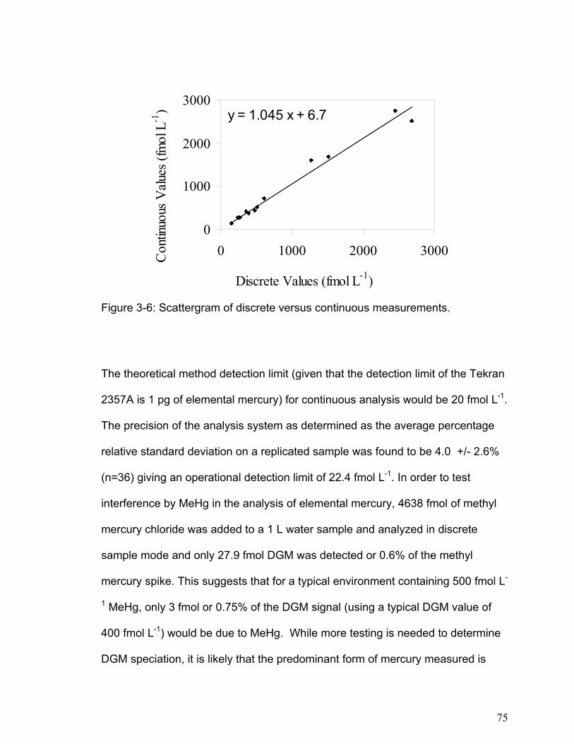
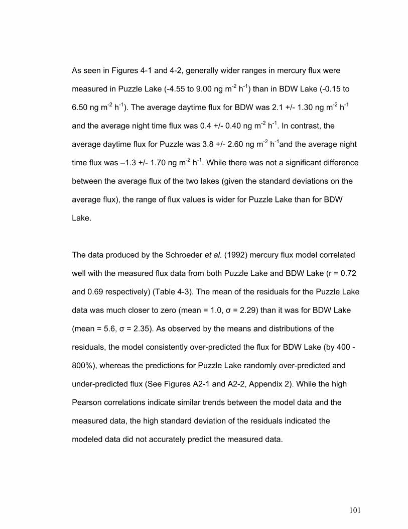
DISSOLVED GASEOUS MERCURY DYNAMICS AND MERCURY VOLATILIZATION IN FRESHWATER LAKES NELSON JAMES O’DRISCOLL Thesis submitted to the Faculty of Graduate and Postdoctoral Studies University of Ottawa in partial fulfillment of the requirements for the Ph.D. degree in the Ottawa-Carleton Institute of Biology Thèse soumise à Faculté des études supérieures et postdoctorales Université d’Ottawa en vue de l’obtention du doctorat L’Institut de biologie d’Ottawa-Carleton
Transcript
DISSOLVED GASEOUS MERCURY DYNAMICS AND MERCURY VOLATILIZATION IN FRESHWATER LAKES
NELSON JAMES O’DRISCOLL
Thesis submitted to the Faculty of Graduate and Postdoctoral Studies
University of Ottawa in partial fulfillment of the requirements for the
Ph.D. degree in the
Ottawa-Carleton Institute of Biology
Thèse soumise à Faculté des études supérieures et postdoctorales
Université d’Ottawa en vue de l’obtention du doctorat
L’Institut de biologie d’Ottawa-Carleton
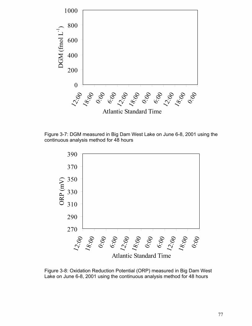
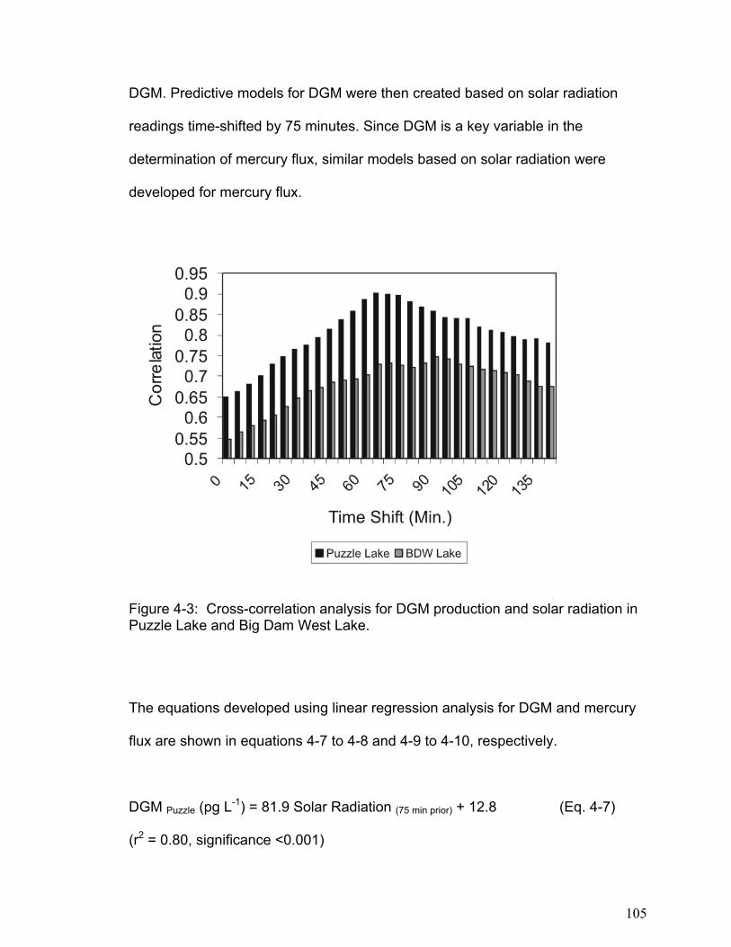
Abstract This thesis examines the production and distribution of dissolved gaseous mercury (DGM) in freshwater ecosystems and its relationship to mercury volatilization. The importance of volatilization was assessed within a multidisciplinary mercury mass balance for Big Dam West Lake (BDW) Kejimkujik Park, Nova Scotia. The magnitude of volatilization was found to be approximately double the direct wet deposition over lake and wetlands, and 27% of the direct wet deposition to the terrestrial catchment. Over the entire basin area the mass of mercury volatilized is 46% of the mass deposited by wet deposition. A new method of continuous (5 minute) DGM analysis was developed and tested. The detection limit for DGM was 20 fmol L-1 with 99% removal efficiency. Control experiments showed that there was no interference due to methyl mercury, which is present in similar concentrations to DGM. Experiments comparing continuous DGM analysis with discrete DGM analysis showed that the results are not significantly affected by typical variations in water temperature (4- 30 o C), oxidation-reduction potential (135-355 mV), dissolved organic carbon (4.5- 10.5 mg L-1), or pH (3.5- 7.8). The continuous analysis was within 4.5% of the discrete analysis when compared across 12 samples analyzed in triplicate. Diurnal patterns for dissolved gaseous mercury (DGM) and mercury flux were measured (using this new DGM method and a Teflon flux chamber method) in two lakes with contrasting dissolved organic carbon (DOC) concentrations in Kejimkujik Park, Nova Scotia. Consistently higher DGM concentrations were found in the high DOC lake as compared to the low DOC lake. Cross-correlation analysis indicated that DGM dynamics changed in response to solar radiation with lag-times of 65 and 90 minutes. An examination of current mercury flux models using this quantitative data indicated some good correlations between the data and predicted flux (r ranging from 0.27 to 0.83) but generally poor fit (standard deviation of residuals ranging from 0.97 to 3.38). This research indicates that DOC and wind speed may play important roles in DGM and mercury flux dynamics that have not been adequately accounted for in current predictive models. The link between DOC concentrations and DGM production was further investigated using tangential ultrafiltration to manipulate DOC concentrations in water samples. In this way, a range of samples with different DOC concentrations was produced for each lake without substantial changes to DOC structure or dissolved ions. This was repeated for four lakes in northern Quebec; two with drainage basins that were extensively logged and two drainage basins were minimally logged. On two separate days for each lake, abiotic water samples of varying DOC concentrations were incubated in clear and dark Teflon bottles on the lake surface with temperature and DGM concentrations measured
2
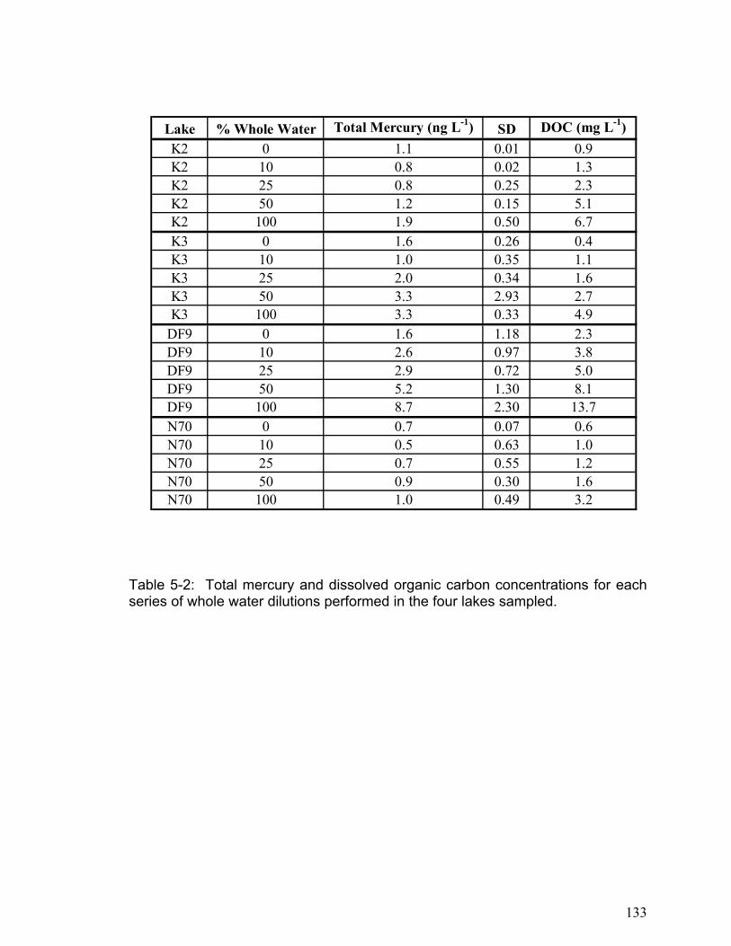
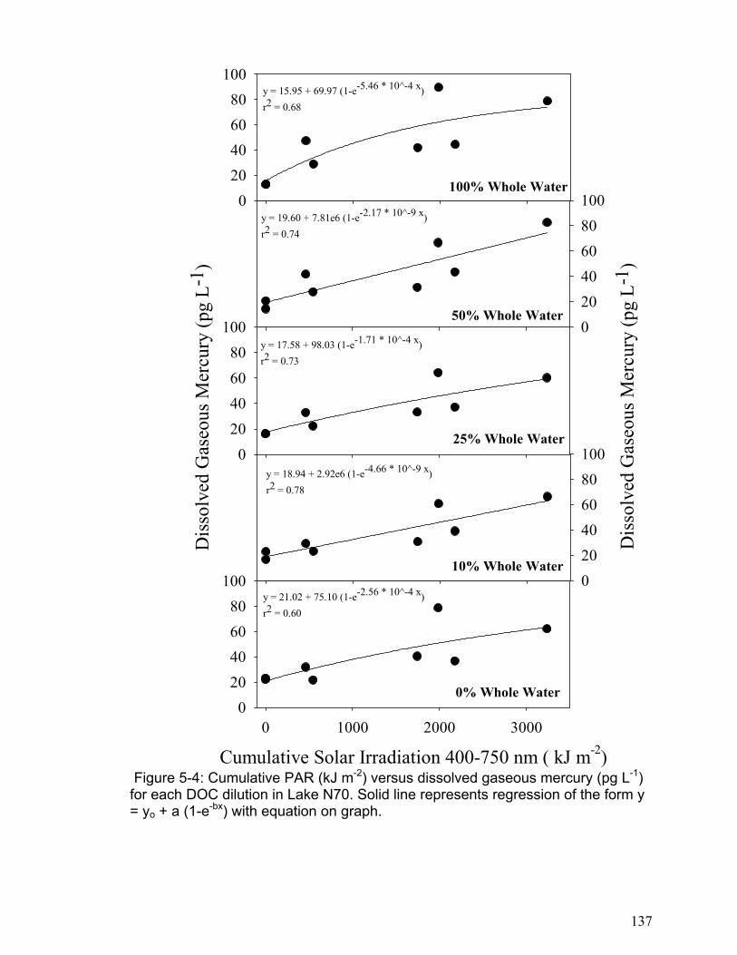
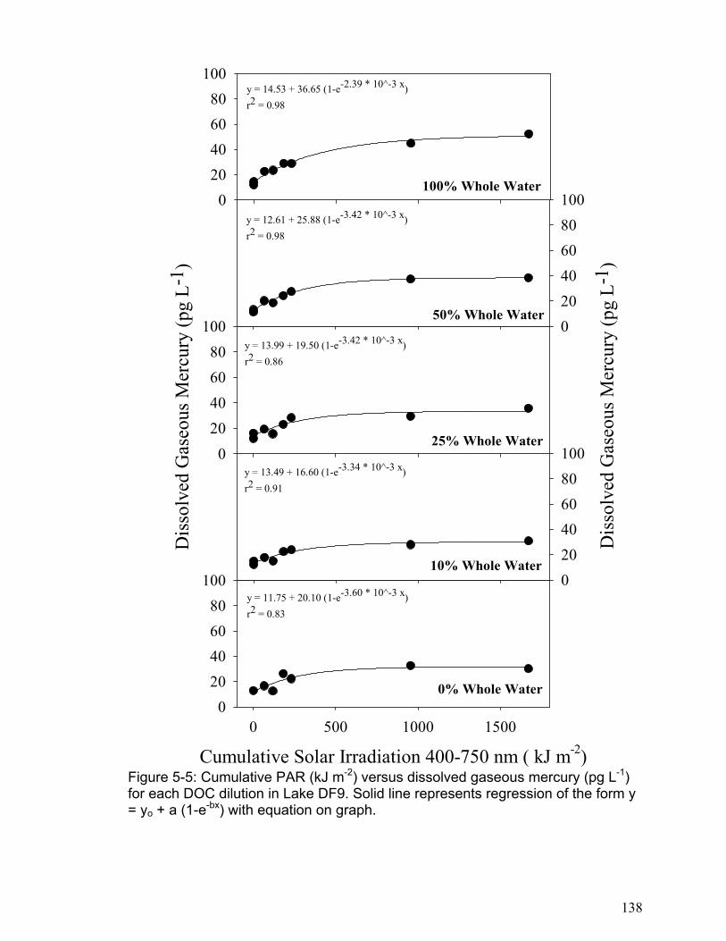
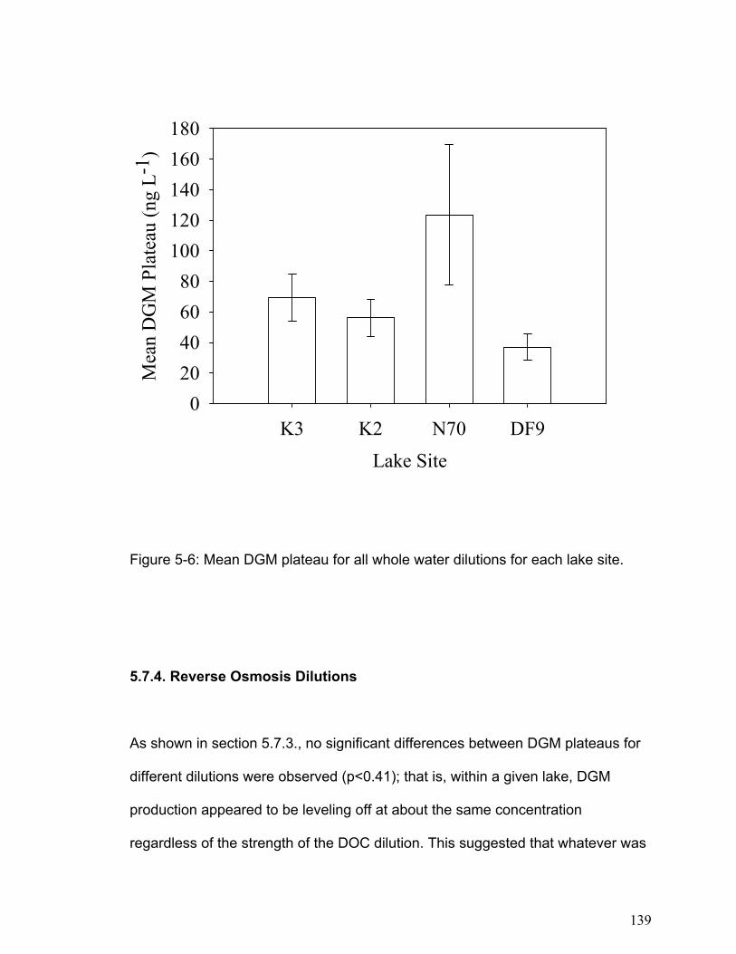
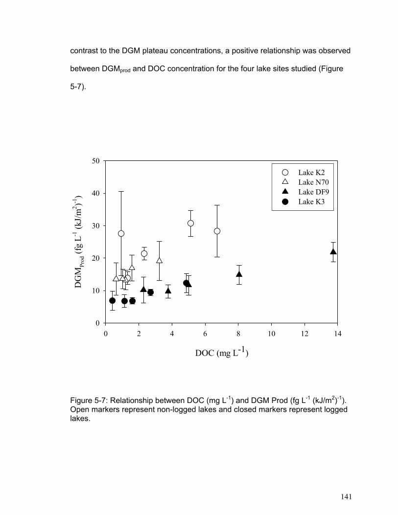
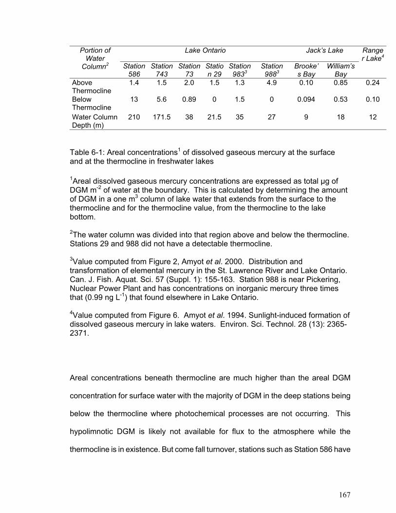
at 3.5-hour intervals over the course of 10.5 hours. Levels of DGM increased with increasing cumulative irradiation for all lakes until approximately 4000 kJ m-2 (400-750 nm, photosynthetically active radiation (PAR)), when DGM concentration reached a plateau (between 20 and 200pg L-1). Assuming that DGM production was limited by the amount of photo-reducible mercury, reversible first-order reaction kinetics fit the observed data well (r2 ranging from 0.59 to 0.98). The DGM plateaus were independent of DOC concentrations but differed between lakes. In contrast photo-production efficiency (DGMprod), i.e. the amount of DGM produced per unit radiation (fg L-1 (kJ/m2)-1) prior to 4000 kJ m-2 PAR, was linearly (P<0.0005) proportional to DOC concentration. Furthermore, logged lakes had a lower (P<0.006) DGMprod per unit DOC than the non-logged lakes. In these four lakes, the rate of DGM production per unit PAR was dependent on the concentration of DOC, with significant differences between lakes presumably due to different DOC structures and dissolved ions. The distribution of DGM in the water columns of shallow and deep freshwater lakes was investigated in lake Ontario and several small freshwater lakes. When DGM concentrations were expressed on an areal basis, DGM concentrations above the thermocline in Lake Ontario average 1.5 ng m-2 and in small freshwater lakes it ranged between 0.1 and 0.8 ng m-2. Further, it was demonstrated that the majority of DGM in large freshwater lakes such as Lake Ontario exists below the thermocline where photochemical oxidation and reduction processes cannot occur. The depth profiles indicate that vertical mixing in the water column may alter the DGM concentration in the upper epilimnion, and that turn over in deep lakes may result in a transfer of large concentrations of DGM from the hypolimnion into the epilimnion. In addition, the results indicate that microbial processes may be an important factor regulating DGM in the water column of freshwater lakes, particularly in the hypolimnion.
3
Résumé
La production et la distribution du mercure gazeux dissous (DGM) dans des écosystèmes d'eau douce ainsi que son rapport avec la volatilisation du mercure ont été étudiés. L'importance de la volatilisation a été évaluée dans un bilan de masse du mercure multidisciplinaire pour le lac Big Dam West (BDW) dans le parc Kejimkujik, en Nouvelle-Écosse. L'ampleur de la volatilisation s'est avérée approximativement le double du dépôt humide direct au-dessus du lac et des terres humides, et 27% du dépôt humide direct sur le bassin-versant. Au-dessus de la superficie entière du bassin, la masse de mercure volatilisé équivaut à 46% de la masse déposée par dépôt humide. Une nouvelle méthode d'analyse continue de DGM (5 minute d’intervalle) a été développée et examinée. La limite de détection du DGM était de 20 fmol L-1, avec un rendement d’élimination de 99%. Des expériences de contrôle ont démontré qu'il n'y avait aucune interférence due au methyl-mercure, qui est présent en concentrations semblables au DGM. Des expériences comparant l'analyse continue de DGM à l'analyse discrète de DGM ont démontré que les résultats ne sont pas significativement affectés par des variations typiques de la température de l'eau (de 4 à 30oC), du potentiel d'oxydation-réduction (de 135 à 355 mV), du carbone organique dissous (de 4,5 à 10,5 mg L-1), ou du pH (de 3,5 à 7,8). L'analyse continue était à moins de 4.5% de l'analyse discrète lorsque ces deux méthodes ont été comparées à l’aide de 12 échantillons analysés en triplicat. Des cycles diurnaux du flux du mercure gazeux dissous (DGM) et du mercure ont été mesurés (en utilisant la nouvelle méthode pour le DGM et une méthode de chambre de flux en Téflon) dans deux lacs ayant des concentrations différentes de carbone organique dissous (DOC) au parc Kejimkujik en Nouvelle-Écosse. Des concentrations uniformément plus élevées de DGM ont été observées dans le lac ayant une concentration élevée de DOC par rapport au lac dont la concentration de DOC était faible. Une analyse de corrélation croisée a indiqué que la dynamique de DGM change selon le rayonnement solaire, avec des temps de réponse de 65 et 90 minutes. Un examen des modèles courants de flux de mercure en employant ces données quantitatives a indiqué de bonnes corrélations entre le flux observé et le flux prédit (r s'étendant de 0,27 à 0,83) mais l’ajustement était généralement faible (écart type des résidus s'étendant de 0,97 à 3,38). Cette recherche indique que la concentration de DOC et la vitesse du vent peuvent jouer des rôles importants dans la dynamique du flux du DGM et du mercure qui ne sont pas pris en compte adéquatement par les modèles de prévision courants. Le lien entre les concentrations de DOC et la production de DGM a été étudié en utilisant l'ultrafiltration tangentielle permettant de modifier les concentrations de DOC dans des échantillons d'eau. De cette façon, une gamme d’échantillons
4
ayant différentes concentrations de DOC a été produite pour chaque lac sans changements importants à la structure du DOC ou des ions dissous. Ceci a été répété pour quatre lacs au nord du Québec; deux lacs pour lesquels la coupe forestière est importante dans le bassin-versant et deux lacs pour lesquels la coupe forestière dans le bassin-versant est minimale. Des expériences ont été entreprises à deux occasions dans chaque lac. Durant celles-ci, des échantillons abiotiques d'eau ayant des concentrations variées en DOC ont été incubés à la surface du lac dans des bouteilles de Téflon claires et foncées. La température et les concentrations de DGM ont été mesurées à 3,5 heures d’intervalle pendant une periode de 10,5 heures. Dans tous les lacs, les niveaux de DGM ont augmenté avec l'augmentation de l'irradiation cumulative, jusqu'à environ 4000 kJ m-2 (de 400 à 750 nm, rayonnement actif photosynthétique (PAR)), niveau d’irradiation auquel la concentration de DGM atteint un plateau (entre 20 et 200 pg L-1). En supposant que la production de DGM était limitée par la quantité de mercure photo-réductible, la cinétique de réaction réversible de premier ordre ajuste bien les données observées (r2 s'étendant de 0,59 à 0,98). Les plateaux de DGM étaient indépendants des concentrations de DOC mais différaient entre lacs. À l’opposé, l'efficacité de photo-production (DGMprod), c’est-à-dire la quantité de DGM produit par unité de radiation (fg L-1 (kJ/m2)-1) sous 4000 kJ m-2 PAR, était linéairement (P<0,0005) proportionnelle à la concentration de DOC. De plus, les lacs autour desquels la coupe forestière est importante avaient un DGMprod par unité de DOC inférieur (P<0,006) à celui des lacs autour desquels la coupe forestière n’est pas importante. Dans ces quatre lacs, le taux de production de DGM par d'unité de PAR dépendait de la concentration du DOC, avec des différences significatives entre les lacs probablement dues à des structures de DOC et à des ions dissous différents. La distribution de DGM dans la colonne d'eau de lacs d'eau douce peu profonds et profonds a été étudiée dans le lac Ontario et dans plusieurs petits lacs d'eau douce. Lorsque les concentrations de DGM sont exprimées en terme de superficie, les concentrations de DGM au-dessus de la thermocline sont en moyenne 1,5 ng m-2 dans le lac Ontario et elles s’étendent de 0,1 à 0,8 ng m-2 dans les petits lacs d'eau douce. De plus, on a démontré que la majorité du DGM dans de grands lacs d'eau douce tels que le lac Ontario se retrouve sous la thermocline, où les processus photochimiques d'oxydation et de réduction ne peuvent pas se produire. Les profils de profondeur indiquent que la concentration de DGM dans la partie supérieure de l'épilimnion peut être altérée par le mélange vertical dans la colonne d’eau, et que le renversement dans les lacs profonds peut résulter en un transfert de grandes concentrations de DGM de l’hypolimnion à l'épilimnion. Également, les résultats indiquent que les processus microbiens peuvent être un facteur important réglant le DGM dans la colonne d'eau des lacs d'eau douce, en particulier dans l’hypolimnion.
5
Acknowledgements
I want to express my sincere thanks to my supervisor Dr. David Lean for his scientific, financial, and moral support throughout the completion of this thesis. I want to thank my primary collaborator Dr. Steven Siciliano for his guidance and advice on all aspects of the thesis work. I would also like to thank Dr. Andy Rencz and Dr. Jules Blais who were exemplary thesis advisors. Thanks to all the members of the TSRI #124 mercury research team who provided guidance and scientific collaboration throughout my research (in particular Dr. Steven Beauchamp and Rob Tordon for collaboration on the mercury flux work). This research was supported by NSERC and OGSST scholarships to Nelson O’Driscoll as well as NSERC research grants to Dr. David Lean. Additional funding was provided by the Toxic Substances Research Initiative (TSRI) Program, the Collaborative Mercury Research Network (COMERN), and the National Center of Excellence for Sustainable Forestry Management. Thanks to Richard Carignan for collaboration on research at Lake Berthelot. Thanks the staff and crew of the Canadian Coast Guard vessel, Limnos for their assistance in conducting this research. Thanks to Graeme Bonham-Carter and Laurier Poissant for their scientific input on volatilization models data. Thanks to John Murimba and the Chakrabarti Lab at Carleton University for cation and anion analysis. Much thanks also to the many other researchers, grad students, and technicians who were instrumental in helping me with field work and analysis along the way (To name a few: Lisa Loseto, Jonathon Holmes, Mike Russel, Carrie Rickwood, Jonathon Hill, Susan Winch, Jeff Ridel, Marc Amyot, Valbonna Cello, J.P. Riox, Tanya Peron, Deb Kliza, John Buckle, Lee Sorenson, Mike Murphy, Ian Myers, John Hopkins, Don Hopkins, JD Whall, Katherine Kepple Jones, Frank Schaedelich, Melissa Legrand, Maya Spitz, ... and the list goes on) . My final (and largest) thanks are to my wife Claire Wilson O’Driscoll. Without you this thesis would have never been completed. You are my editor, my constant moral support, my role model, and my partner in every sense. This thesis is dedicated to the women in my life who made me the person I am today: Mary O’Driscoll (grandmother), Agnes O’Driscoll (mother), Claire Wilson O’Driscoll (wife), and Ellen O’Driscoll (daughter).
1.1. Thesis Rationale ........................................................................................................................... 18 1.2. A Review of Photo-Reduction and Photo-Oxidation..................................................................... 21 1.3. Limitations of Previous DGM Research ....................................................................................... 24 1.4. Thesis Organization...................................................................................................................... 27
1.4.1. General and Specific Objectives............................................................................................ 27 1.4.2. Thesis Overview and Null Hypotheses.................................................................................. 28
CHAPTER 2 .............................................................................................................................................. 34 MERCURY MASS BALANCE FOR BIG DAM WEST LAKE, KEJIMKUJIK PARK, NOVA SCOTIA: EXAMINING THE ROLE OF VOLATILIZATION.............................................................................. 34
2.3.1 Lakewater & Inflow/Outflow Sampling and Analysis............................................................ 39 2.3.2 Total Mercury in Precipitation................................................................................................ 40 2.3.3. Groundwater Sampling .......................................................................................................... 40 2.3.4. Soil-Air and Water-Air Flux.................................................................................................. 41 2.3.5 Sediment ................................................................................................................................. 42 2.3.6 Vegetation............................................................................................................................... 46 2.3.7. Mercury Conceptual Model ................................................................................................... 47
2.4. Results .......................................................................................................................................... 48 2.4.1. Overview of Mass Balance.................................................................................................... 48 2.4.2. Calculation of Uncertainty..................................................................................................... 52
2.5. Discussion .................................................................................................................................... 53 2.5.1. Comparison of Flux Values to Literature .............................................................................. 53 2.5.2. Relative Magnitude of Fluxes............................................................................................... 54 2.5.3. The Role of Wet Deposition in Volatilization ....................................................................... 56 2.5.4. Sources of Error..................................................................................................................... 57 2.5.5. Summary................................................................................................................................ 59
CHAPTER 3 .............................................................................................................................................. 60 CONTINUOUS ANALYSIS OF DISSOLVED GASEOUS MERCURY IN FRESHWATER LAKES 60
CONTINUOUS ANALYSIS OF DISSOLVED GASEOUS MERCURY (DGM) AND MERCURY FLUX IN TWO FRESHWATER LAKES IN KEJIMKUJIK PARK, NOVA SCOTIA: EVALUATING MERCURY FLUX MODELS WITH QUANTITATIVE DATA........................................................... 82
4.3.1. Continuous analysis of DGM ................................................................................................ 86 4.3.2. Continuous Analysis of Gaseous Elemental Mercury in Ambient Air .................................. 88 4.3.3. Continuous Analysis of Mercury Flux from Water ............................................................... 89 4.3.4. Flux Model Evaluation and Description ................................................................................ 90 3.3.5. Mass Transfer Mercury Flux Model ...................................................................................... 91 4.3.6. Temperature- and Wind-Sensitive Mass Transfer Mercury Flux Models.............................. 92 4.3.7. Solar Radiation and Wind Speed (Empirically-Derived) Mercury Flux Model..................... 93 4.3.8. Empirical Approach with Continuous Data ........................................................................... 93 4.3.9. Site Description ..................................................................................................................... 95
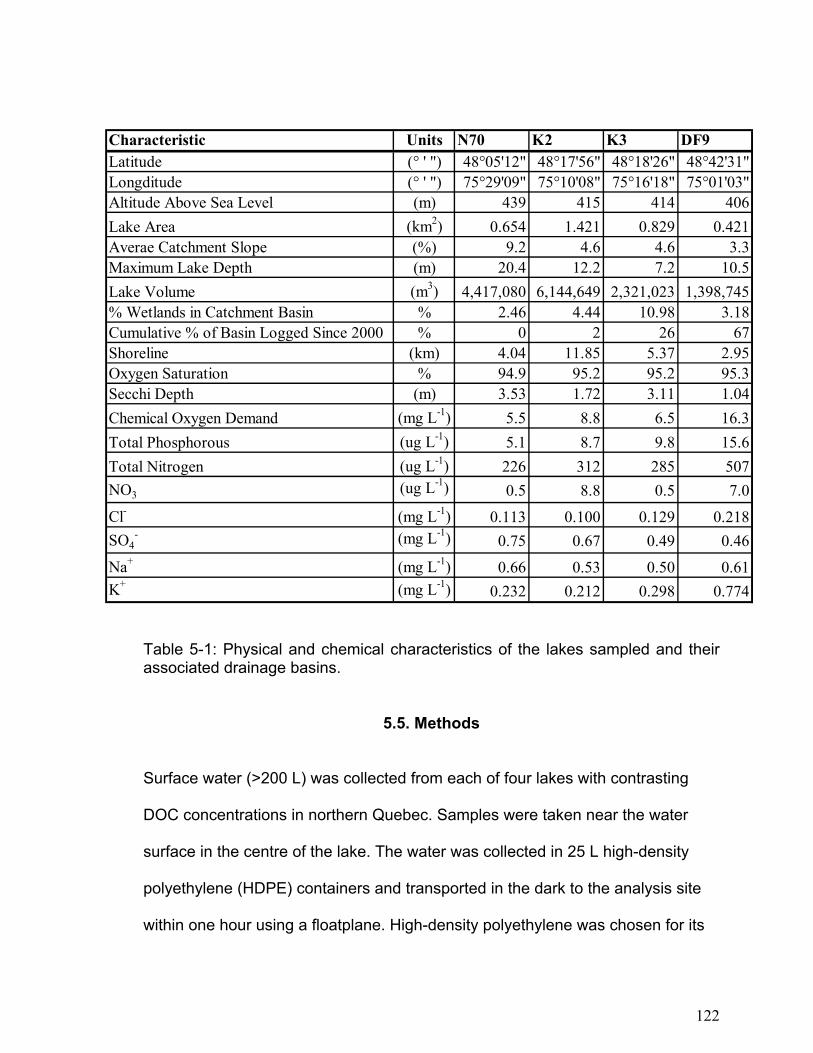
CHAPTER 5 ............................................................................................................................................ 116 EFFECTS OF DISSOLVED ORGANIC CARBON ON THE PHOTO-PRODUCTION OF DISSOLVED GASEOUS MERCURY (DGM) IN FRESHWATER LAKES............................................................. 116
MICROBIAL REDUCTION AND OXIDATION OF HG IN FRESHWATER LAKES..................... 192 Abstract ............................................................................................................................................. 193 Introduction ....................................................................................................................................... 194 Experimental Section......................................................................................................................... 196
Site Description ............................................................................................................................. 196 Analysis of Dissolved Elemental Mercury in Lake Water............................................................. 197 Analysis of Microbial Mercury Reductase and Oxidase Activity.................................................. 198 Hydrogen Peroxide Experiments ................................................................................................... 199
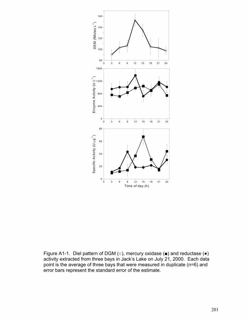
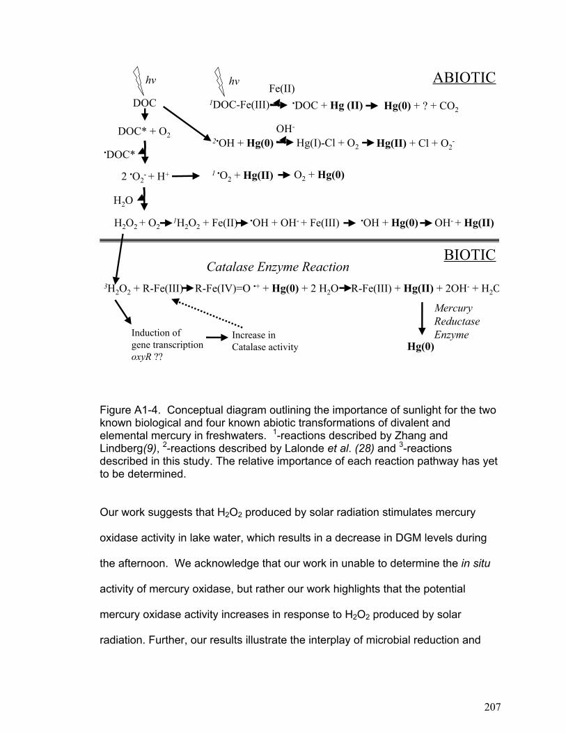
Results and Discussion ...................................................................................................................... 200 Appendix 1 Literature Cited .............................................................................................................. 209
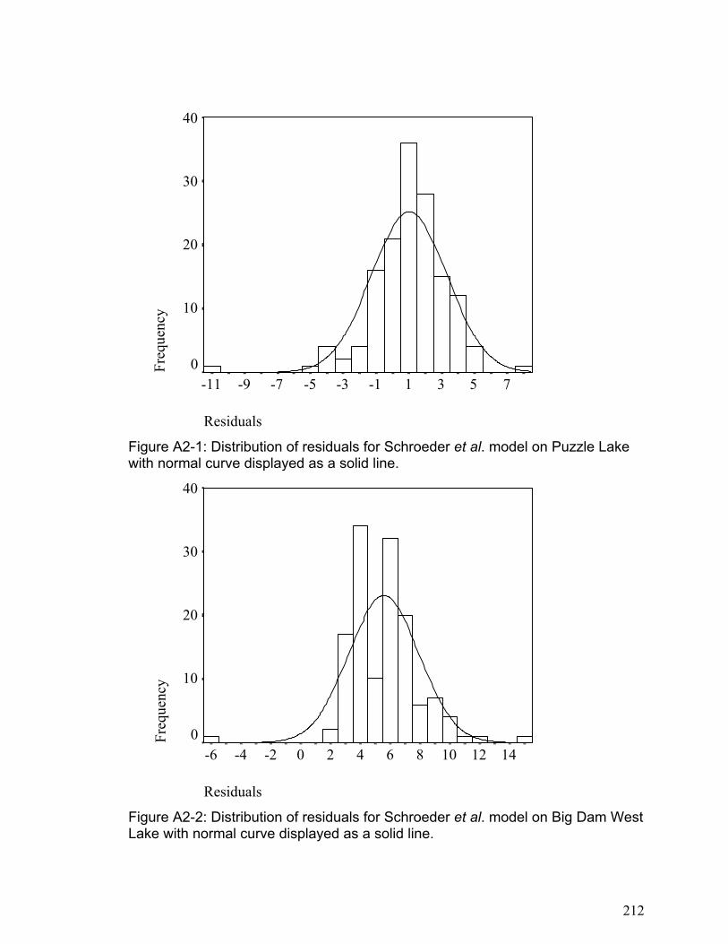
APPENDIX 2 ........................................................................................................................................... 211 SUPPLEMENTARY INFORMATION FOR CHAPTER 4................................................................................... 211
9
List of Figures
Figure 1-1: Conceptual diagram outlining the major processes within the mercury cycle
of freshwater lakes .......................................................................................... 21
Figure 1-2: Conceptual diagram outlining relationship between solar radiation, DGM
formation and mercury volatilization.............................................................. 24
Figure 2-1:Conceptual diagram of mercury cycling in Big Dam West Lake, Kejimkujik
Park, Nova Scotia. Values represent mean mass of mercury flux per year. ... 48
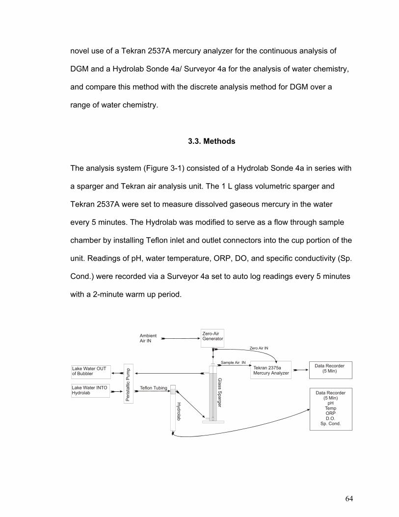
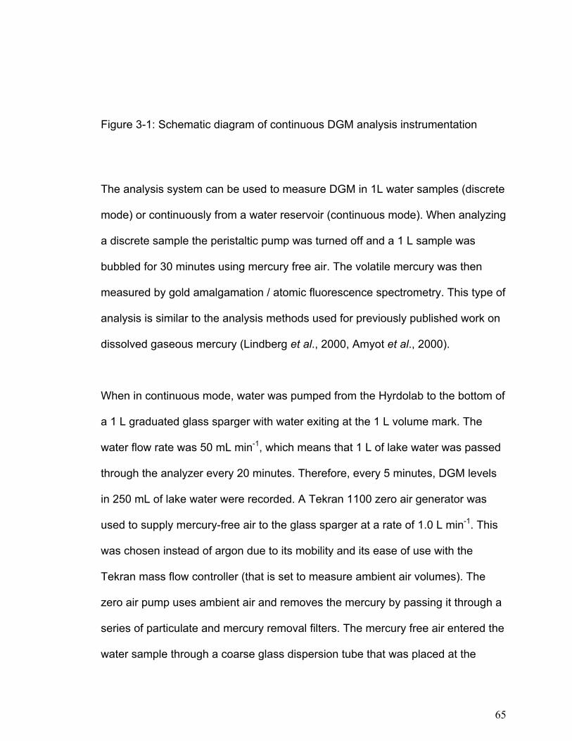
Figure 3-1: Schematic diagram of continuous DGM analysis instrumentation............... 65
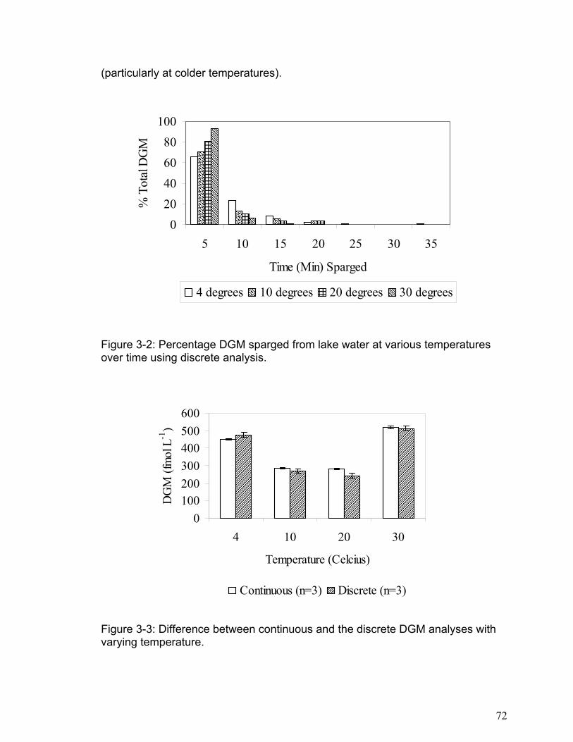
Figure 3-2: Percentage DGM sparged from lake water at various temperatures over time
using discrete analysis..................................................................................... 72
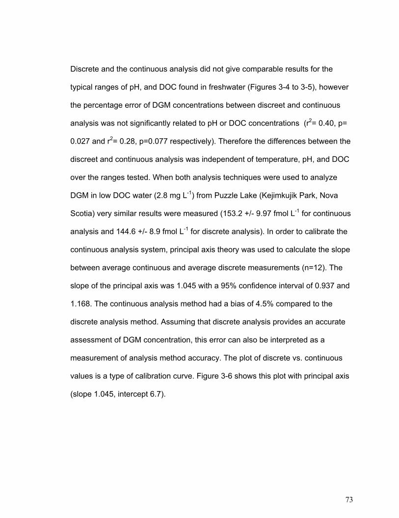
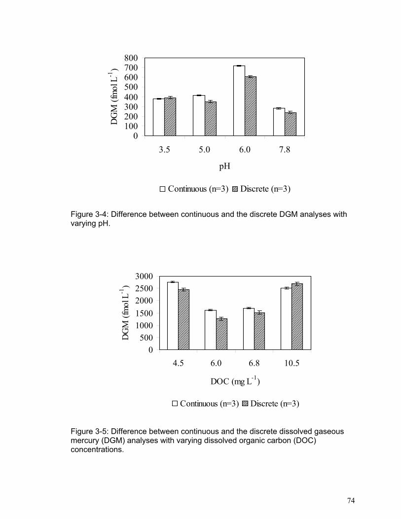
Figure 3-3: Difference between continuous and the discrete DGM analyses with varying
DOC/TOC: Dissolved Organic Carbon / Total Organic Carbon
GEM: Gaseous Elemental Mercury
GIS: Geographic Information System
GMT: Greenwich Mean Time
HDPE/LDPE: High Density Polyethylene / Low Density Polyethylene
IR: Infra Red
MDN: Mercury Deposition Network
MeHg: Methyl Mercury
NADP: National Atmospheric Deposition Program
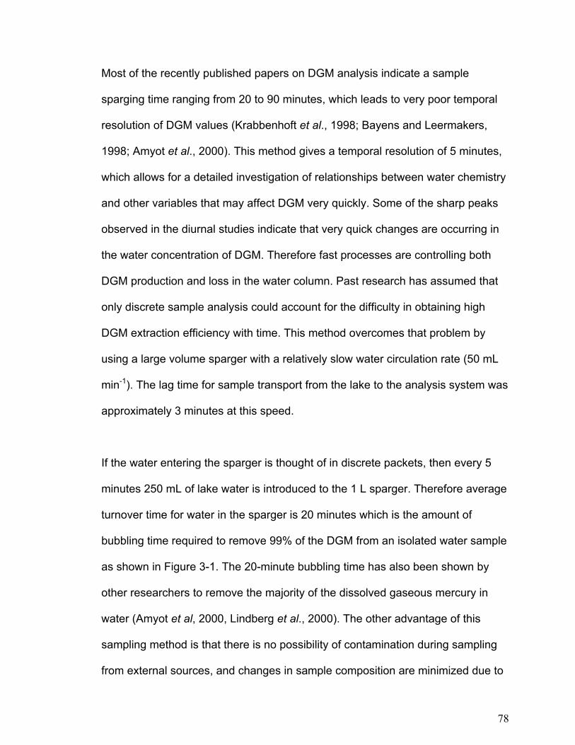
ORP: Oxidation-Reduction Potential
PAR: Photo synthetically Active Radiation
QA/QC: Quality Assurance / Quality Control
RSD: Relative Standard Deviation
SOP: Standard Operating Protocol
TADS: Tekran Automated Dual Sampling System
USEPA: United States Environmental Protection Agency
UV: Ultra Violet
16
Chapter 1
Introduction
17
1.1. Thesis Rationale
Mercury is an important environmental contaminant that bioaccumulates in food
chains and causes severe health effects in aquatic predators and the human
populations that consume them. Mercury pollution first received worldwide
attention with the Minimata Bay disaster in Japan in 1956, when large numbers of
fisherman near the Chisso Chemical Company plant were diagnosed with
neurological disorders (Takizawa & Osame, 2001). Since then, it has been
shown that environmentally realistic concentrations of mercury decrease the
reproductive success of some fish populations (eg. Hammerschmidt et al. 2002),
and that elevated levels of mercury in fish-eating birds can severely reduce clutch
sizes and hatchability as well as increasing hatchling mortality (Wolfe et al.,
1998). Human populations particularly at risk for mercury poisoning are those that
consume large amounts of fish, such as aboriginal peoples (Wheatley and
Paradis, 1995). Effects of mercury exposure in humans include immunotoxicity
(Sweet and Zelikoff, 2001) and neurological damage characterized by ataxia,
sensory disturbances and changes in the mental state (Chang, 1987).
Elevated levels of mercury in biota are present not only in contaminated sites but
also in relatively remote freshwater lakes. For example, Kejimkujik Park in Nova
Scotia has no direct anthropogenic inputs of mercury and yet has loons with the
highest blood mercury concentrations in North America (Burgess et al., 1998;
Evers et al., 1998). Likewise, many fish in other remote lakes have been found to
have elevated mercury levels in tissue (Sorensen et al., 1990; Lathrop et al.,
18
1991; Cabana et al., 1994).
The key to understanding mercury dynamics in the environment is a more
detailed knowledge of the mercury cycle. Indeed, both the US-EPA and Health
Canada have identified the study of mercury cycling in the environment as a top
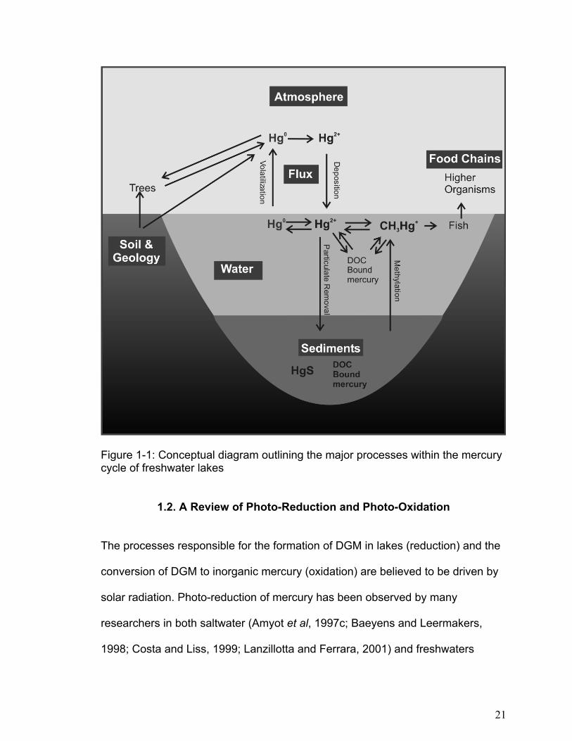
research priority (USEPA, 1997). There are several forms of mercury and a
variety of processes implicated in the mercury cycle (Figure 1-1). The three major
species of mercury are elemental mercury (Hg0), inorganic mercury (Hg2+), and
methyl mercury (CH3Hg+). Elemental mercury is volatile and the main form of
mercury found in the atmosphere, while inorganic mercury is the predominant
form found in water, bound to various organic and inorganic ligands. Methyl
mercury is the form of mercury that bioaccumulates in the food chain. Very low
methyl mercury levels in water (< 0.1 ng L-1) can result in concentrations in higher
trophic levels that exceed human consumption guidelines (> 0.5 µg g-1 wet
weight) (Morel et al., 1998).
One important process in the mercury cycle is the creation of dissolved gaseous
mercury (DGM) in freshwater lakes and its loss to the atmosphere by
volatilization. DGM is believed to consist primarily of elemental mercury (Hg0)
formed from inorganic mercury through the process of reduction (O’Driscoll et al.,
2003b). DGM is the form in which mercury volatilizes from water to air, and
volatilization is one of the primary means of mercury removal from an ecosystem.
19
Mercury volatilization has not been studied in detail in a diversity of ecosystems,
but several researchers have indicated in a general way that it is a significant part
of the mercury cycle. For example, Rolfhus and Fitzgerald (2001) found that
mercury volatilization from Long Island Sound was equivalent to 35% of total
annual mercury inputs to the system, and studies on the Great Lakes show that
mercury volatilization is equivalent to as much as 50% of the total mercury inputs
(Mason and Sullivan, 1997; Watras et al., 1995). In other studies, Mason et al.
(1994) and Amyot et al. (1994) found that mercury volatilization and wet
deposition were close to being in balance. Volatilization has also been shown to
be an important factor in the global distribution of mercury, and Mason et al.
(1994) indicate that mercury volatilization from the ocean surface may account for
approximately 30% of the total global mercury emissions to the atmosphere.
The overall result of DGM formation and volatilization is a reduction in the
mercury burden of freshwater lakes. A reduction in total mercury may ultimately
result in less formation of methyl mercury and therefore in a reduction of mercury
poisoning in the food chain (Nriagu, 1994; Morel et al., 1998). A better
understanding of the factors that affect DGM formation and its relation to
volatilization may help to identify areas at risk for mercury bioaccumulation. This
research may also help to increase the accuracy of global distribution models for
mercury.
20
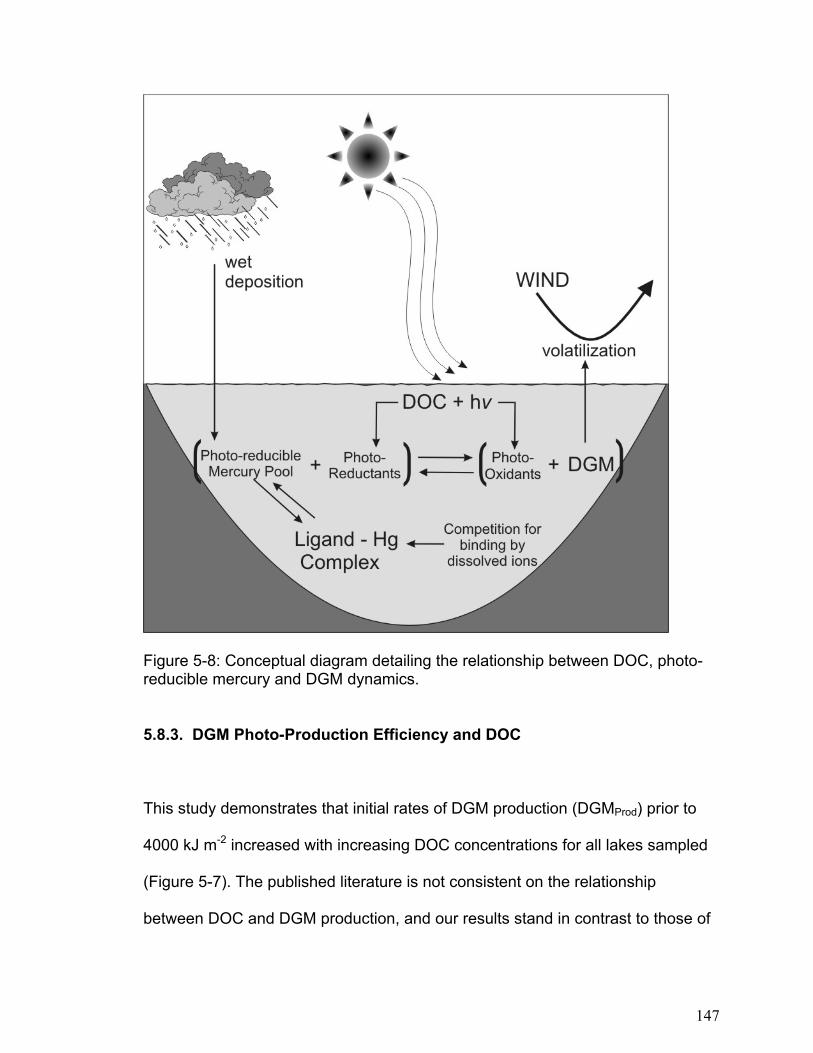
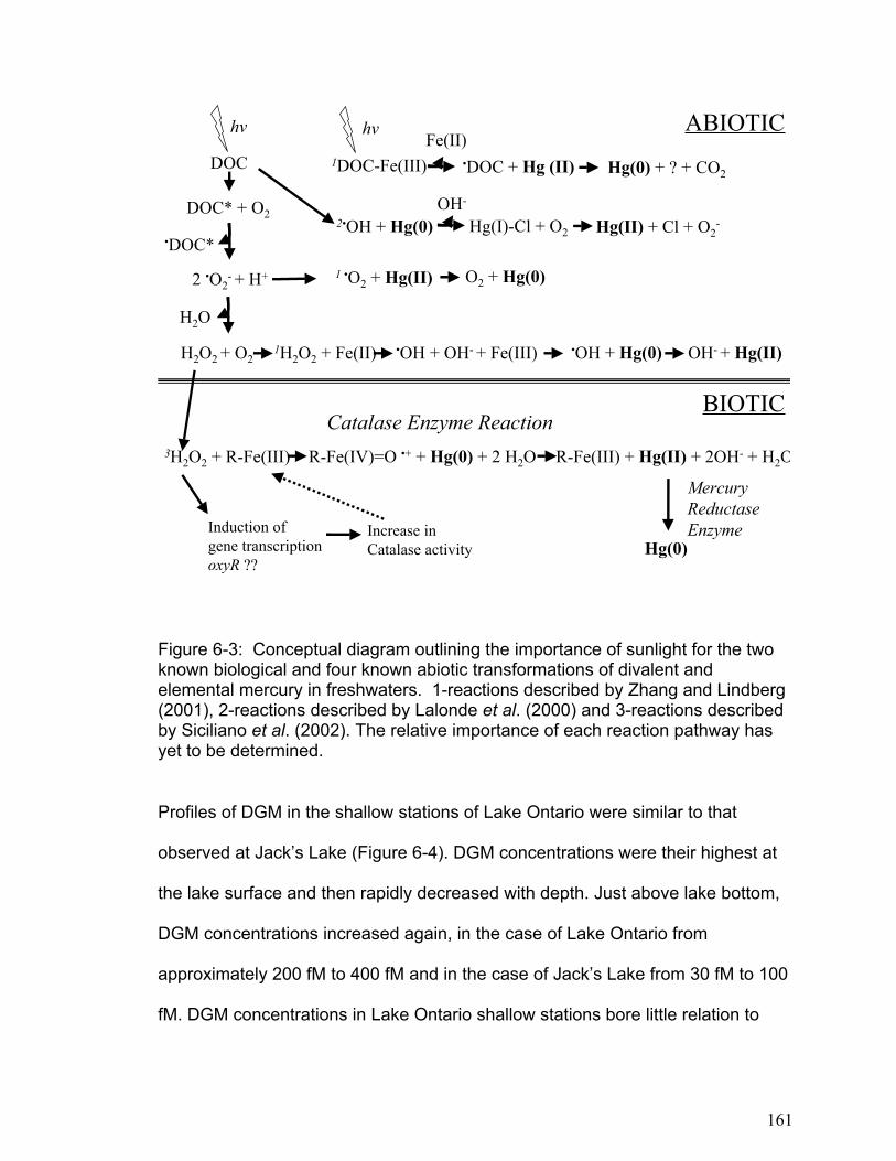
Figure 1-1: Conceptual diagram outlining the major processes within the mercury cycle of freshwater lakes
1.2. A Review of Photo-Reduction and Photo-Oxidation
The processes responsible for the formation of DGM in lakes (reduction) and the
conversion of DGM to inorganic mercury (oxidation) are believed to be driven by
solar radiation. Photo-reduction of mercury has been observed by many
researchers in both saltwater (Amyot et al, 1997c; Baeyens and Leermakers,
1998; Costa and Liss, 1999; Lanzillotta and Ferrara, 2001) and freshwaters
21
(Zhang and Lindberg, 2001; Amyot et al., 1994, 1997a), in temperate lakes and
rivers (Vandal et al., 1991; Amyot et al., 1994, 1997a, 2000), Artic lakes (Amyot
et al., 1997b), and southern wetlands (Krabbenhoft et al., 1998), yet the
mechanisms by which it occurs are not well understood.
Both abiotically- and biotically-mediated mechanisms for photo-reduction have
been suggested in the literature. Nriagu (1994) outlined various abiotic
mechanisms including homogeneous photolysis, reduction by inorganic
particulates and organic molecules, as well as transient reductants. More recently
Zhang and Lindberg (2001) have suggested that iron(III) mediated photo-
reduction is a significant mechanism in DGM formation.
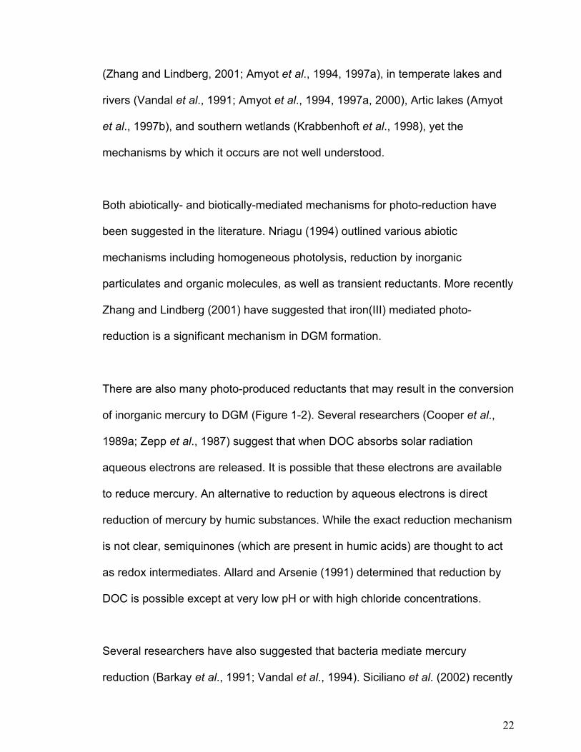
There are also many photo-produced reductants that may result in the conversion
of inorganic mercury to DGM (Figure 1-2). Several researchers (Cooper et al.,
1989a; Zepp et al., 1987) suggest that when DOC absorbs solar radiation
aqueous electrons are released. It is possible that these electrons are available
to reduce mercury. An alternative to reduction by aqueous electrons is direct
reduction of mercury by humic substances. While the exact reduction mechanism
is not clear, semiquinones (which are present in humic acids) are thought to act
as redox intermediates. Allard and Arsenie (1991) determined that reduction by
DOC is possible except at very low pH or with high chloride concentrations.
Several researchers have also suggested that bacteria mediate mercury
reduction (Barkay et al., 1991; Vandal et al., 1994). Siciliano et al. (2002) recently
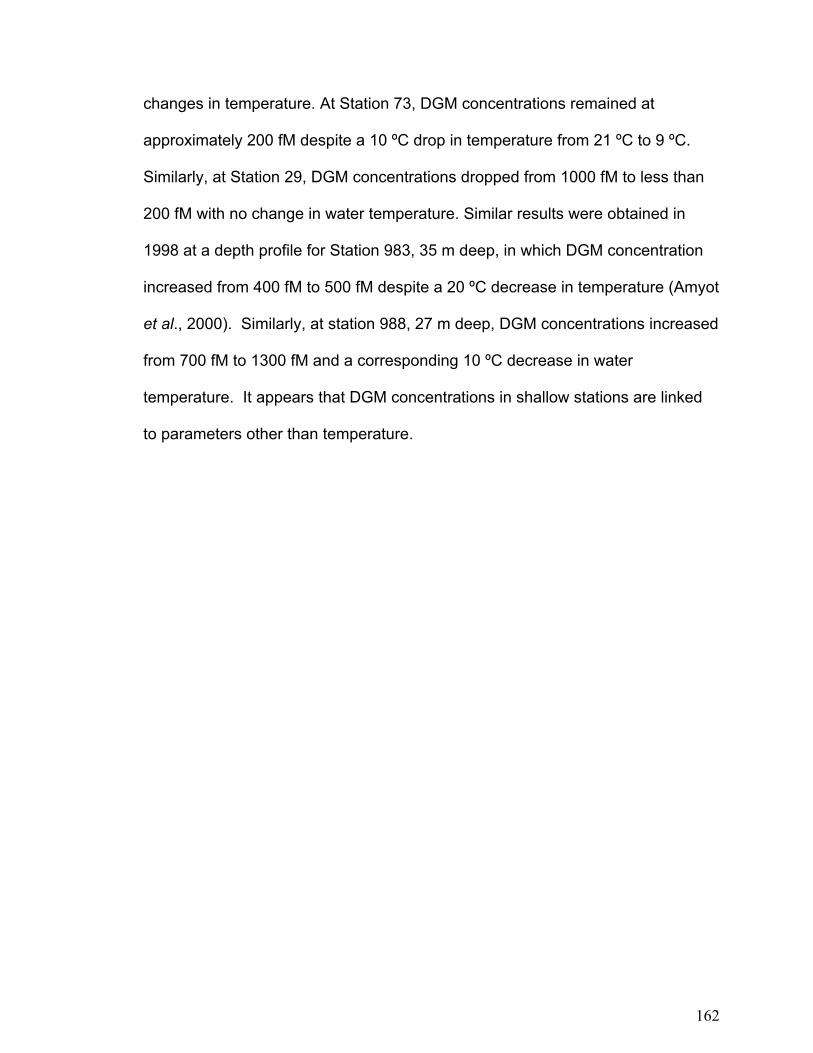
22
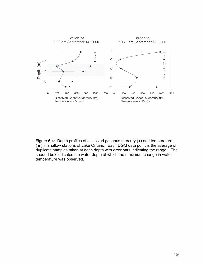
examined the role of microbial reduction and oxidation processes in regulating
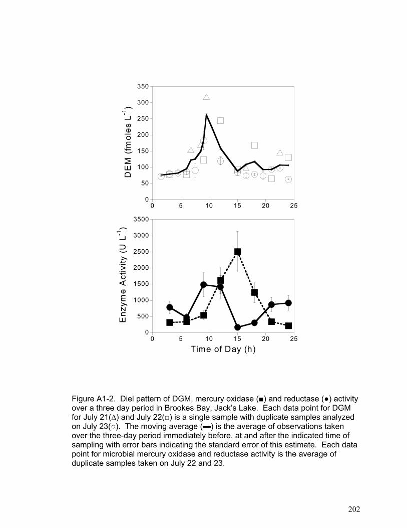
DGM diel patterns in freshwater lakes (Appendix 1). We showed that photo-
chemically produced hydrogen peroxide regulates microbial oxidation processes
and may account for the diel patterns observed in DGM data (Appendix 1).
Overall, the mechanisms responsible for mercury reduction and the relative
contributions of biotic and abiotic processes are still unclear.
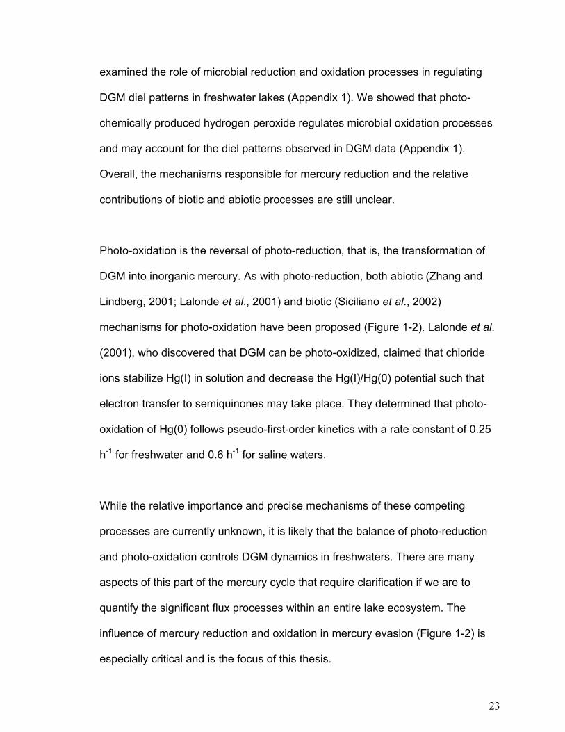
Photo-oxidation is the reversal of photo-reduction, that is, the transformation of
DGM into inorganic mercury. As with photo-reduction, both abiotic (Zhang and
Lindberg, 2001; Lalonde et al., 2001) and biotic (Siciliano et al., 2002)
mechanisms for photo-oxidation have been proposed (Figure 1-2). Lalonde et al.
(2001), who discovered that DGM can be photo-oxidized, claimed that chloride
ions stabilize Hg(I) in solution and decrease the Hg(I)/Hg(0) potential such that
electron transfer to semiquinones may take place. They determined that photo-
oxidation of Hg(0) follows pseudo-first-order kinetics with a rate constant of 0.25
h-1 for freshwater and 0.6 h-1 for saline waters.
While the relative importance and precise mechanisms of these competing
processes are currently unknown, it is likely that the balance of photo-reduction
and photo-oxidation controls DGM dynamics in freshwaters. There are many
aspects of this part of the mercury cycle that require clarification if we are to
quantify the significant flux processes within an entire lake ecosystem. The
influence of mercury reduction and oxidation in mercury evasion (Figure 1-2) is
especially critical and is the focus of this thesis.
23
Figure 1-2: Conceptual diagram outlining relationship between solar radiation, DGM formation and mercury volatilization.
1.3. Limitations of Previous DGM Research
As outlined in the previous section, several studies have identified DGM
volatilization as a significant portion of the mercury cycle (Mason et al., 1994;
Amyot et al., 1994; Watras et al., 1995; Mason and Sullivan, 1997; Rolfhus and
Fitzgerald, 2001). While some mercury mass balances have included values for
volatilization, most studies to date have been pieced together using disparate
data, literature values and theoretical modeling. None have investigated the
importance of mercury volatilization using primary data within a multidisciplinary
24
mass balance model. While volatilization of DGM is thought to be an important
process determining the distribution of mercury, very little research has directly
measured DGM diurnal dynamics in relation to volatilization.
Partly responsible for this are the difficulties presented in the analysis of DGM.
Typically, DGM in freshwater is present at concentrations that are 5 - 20 % that of
total mercury (Amyot et al., 2000). While the total amount of mercury present in
pristine lake water is in the ng L-1 range, the amount that is elemental mercury is
much less (20 - 200 pg L-1 range). The accurate measurement of such small
quantities is difficult, and this has been one of the challenges in performing DGM
research. Another difficulty has been the measurement of fast changes in DGM.
Analysis times typically range from 20 – 90 minutes (Amyot et al., 2000; Lindberg
et al., 2000), while DGM concentrations may change within minutes (O’Driscoll et
al., 2003b). In order to see realistic changes in DGM, an analysis method that
can measure low pg L-1 quantities in a very short time-span is required.
Many researchers have recognized the importance of DGM dynamics and
volatilization in theoretical mercury fate models (Rolfhus and Fitzgerald, 2001;
Mason and Sullivan, 1997; Watras et al., 1995), particularly with regard to the
global cycling of mercury (Mason et al., 1994). While a number of predictive
models for mercury volatilization have been proposed, no work to date has
measured DGM and volatilization simultaneously, nor have they measured
meteorological variables that may have an important influence on DGM dynamics
and mercury flux. Therefore, current theoretical mercury flux models have not
25
been tested or calibrated against quantitative data sets.
There are several factors that are thought to affect DGM formation and
distribution within a lake. One such factor is DOC and the role it plays in DGM
formation. The relationship between DOC and DGM is not consistent in the
published literature, with some authors reporting a positive relationship (O’Driscoll
et al., 2003b; Xiao et al., 1995) and some reporting a negative relationship
(Amyot et al., 1997a; Watras et al., 1995). Part of the confusion may be due to
the confounding effects of DOC structure and dissolved ions on mercury photo-
reduction and photo-oxidation processes. To date no study has attempted to
control changes in DOC structure and dissolved ions while working with natural
freshwater samples. This is likely because it is difficult to alter DOC
concentrations without substantially changing the other chemical constituents
(cations, anions, nutrients) present in lake water. More information on the
complex role that DOC plays in mercury cycling is essential to quantifying the fate
of mercury in ecosystems.
Finally, another important factor that has not been adequately explored is the
distribution of DGM in the water column. A few researchers have attempted a
limited number of depth profiles for DGM, however no clear observations have
emerged (Amyot et al., 1994; 1997a; 1997c). The distribution of DGM in both
shallow and deep freshwater lakes has not been examined, nor have areal
differences in DGM between the epilimnion and the hypolimnion. An
understanding of DGM distribution in the water column is required in order to
26
build whole-lake models for mercury volatilization that incorporate the effects of
water column mixing.
1.4. Thesis Organization
This thesis attempts to address the limitations in current DGM and mercury flux
research that are outlined in Section 1.3. The following is a statement of the
general and specific objectives of the thesis, followed by an overview of chapters
2-6 and the null hypotheses tested in each.
1.4.1. General and Specific Objectives
General Objectives
The general objective of this research is to contribute to a better understanding of
mercury flux processes in the following ways:
• Through the examination of mercury volatilization within a mercury
mass balance for Big Dam West Lake in Kejimkujik Park, Nova Scotia,
using data collected in collaboration with the multidisciplinary research
team supported by the Toxic Substances Research Initiative from
1999-2002;
• Through the development of an improved methodology for the
continuous analysis of dissolved gaseous mercury (DGM) in freshwater
lakes;
• Through a series of studies focused on factors that affect DGM
27
formation and distribution, and on the relationship between these and
mercury volatilization (loss from the ecosystem).
Specific Objectives
• The creation of a mass balance model using quantitative data, to examine
the relative importance of mercury volatilization in the Big Dam West Lake
ecosystem (Chapter 2);
• The development of a method for the near-continuous analysis of DGM
and water chemistry that can be used in remote locations (Chapter 3);
• Examination of the role of DGM in mercury volatilization from lakes, and
specifically the quantification of relationships between DGM, water
chemistry variables, meteorological variables, and mercury volatilization
over a diurnal cycle (Chapter 4);
• Quantification of the relationship between DOC concentration and DGM
photo-production in freshwater, and the development of a logical model
based on field measurements (Chapter 5);
• Examination of trends in DGM distribution through the water columns of
shallow and deep lakes, and the implications for whole-lake modeling of
DGM dynamics (Chapter 6).
1.4.2. Thesis Overview and Null Hypotheses
This thesis consists of five papers (chapters 2-6), each one of which tests a
28
series of hypotheses stemming from one of the specific objectives outlined above
(Section 1.4.1). It should be noted that since each paper has its own introduction
and conclusions, the overall introduction and conclusions of the thesis (Chapters
1 and 7) have been kept intentionally brief to avoid redundancy. An overview of
Chapters 2-6 and the hypotheses they test is provided below.
Chapter 2 describes a multidisciplinary mass balance model of mercury cycling
developed for Big Dam West Lake in Kejimkujik Park Nova Scotia, and examines
the importance of mercury volatilization within this cycle. The following null
hypothesis was tested:
C
t
f
HD H Hm
H02-1: DGM production and volatilization to the atmosphere is not a significant loss process in the mercury cycle of Big Dam West Lake over the course of a year.
hapter 3 details the development, quality assurance/ quality control, and field-
esting of a new methodology for the continuous analysis of DGM in-situ. The
ollowing null hypotheses were tested:
03-1: Continuous measurements of DGM do not calibrate well with discrete GM measurements.
03-2: Methyl mercury does not interfere with DGM measurement.
03-3: Temperature, ORP, DOC and pH will not alter continuous DGM easurements in comparison to discrete measurements.
29
The results of Chapter 3 made it possible to collect the continuous DGM data
outlined in Chapter 4 of the thesis. Chapter 4 investigates the relationships
between DGM, mercury volatilization, water chemistry and meteorological
variables over a diurnal cycle in two freshwater lakes. The data presented here is
also used to test some of the existing theoretical models for mercury flux. The
following null hypotheses were tested:
H04-1: Diurnal dynamics of DGM and mercury volatilization are not correlated with solar radiation. H04-2: There is no time lag between solar radiation measurements and changes in DGM concentration over a diurnal cycle. H04-3: Current mercury flux models accurately predict the relationship between DGM, meteorological variables, and mercury flux. H04-4: Water chemistry and meteorological parameters are not useful predictors of DGM dynamics.
The results of Chapter 4 indicated that current mercury flux models do not
accurately predict diurnal dynamics. However, these models may be improved by
the incorporation of time-shifted solar radiation values and inter-site differences
such as DOC concentration. It was also observed that the high-DOC lake
consistently had higher concentrations of DGM in the surface water than the low-
DOC lake over a diurnal cycle. The effects of DOC on DGM dynamics are not
well understood, with conflicting opinions presented in the published literature. It
was therefore decided to examine this in more detail.
30
Chapter 5 examines the effects of DOC concentration on DGM photo-production
in four freshwater lakes in northern Quebec. Two of the lakes are in logged
catchments, while two are in catchments where little or no logging has taken
place. The following null hypotheses were tested:
H05-1: Changes in DGM concentration are not related to cumulative solar radiation. H05-2: The DGM plateau is not related to changes in DOC concentration. H05-3: The initial DGM production rate is not related to changes in DOC concentration. H05-4: DGM photo-production cannot be accurately modeled as a reversible reaction based on the photo-reduction of the photo-reducible mercury fraction. H05-5: The initial DGM photo-production rate is not different between logged and non-logged freshwater lakes.
The results of chapter 5 indicated that DGM photo-production increases linearly
with solar radiation in all lakes to a point (approximately 4000 kJ m-2 cumulative
PAR), and then it levels to a plateau. The DGM photo-production results were
accurately modeled using kinetic equations based on a first order reversible
reaction. The DGM plateaus were not related to DOC concentrations, but the
initial DGM production rate was significantly related to DOC concentration in each
lake. In addition, the logged lakes were found to have lower rates of initial DGM
production. This indicates that logging may reduce a lake’s ability to produce
DGM and thus result in an increase in a lake’s mercury pool. One important
31
caveat for the presented results is that the experiments were performed on
surface water. In a whole-lake DGM model, the effects of water column mixing
and solar attenuation would have to be taken into account.
Chapter 6 examines the DGM distribution in the water columns of freshwater
lakes. An understanding of DGM distribution with depth is essential to creating
whole-lake models of mercury volatilization that account for the effects of water
column mixing on DGM dynamics. The following null hypotheses were tested:
H06-1: There are no differences between areal DGM concentrations in small and large lakes. H06-2: There are no differences between the areal DGM concentrations above and below the thermocline of large and small lakes. H06-3: Microbial oxidation and reduction processes are not important to the distribution of DGM in the water column.
The results in Chapter 6 show that the small freshwater lakes examined had
lower areal DGM concentrations than lake Ontario. Furthermore, in large
freshwater lakes the majority of DGM exists below the thermocline where photo-
induced oxidation and reduction processes cannot occur. This supports the
theory that microbial reduction processes may be important in DGM production.
This area of study is further examined in a co-authored paper that is included as
Appendix 1. The results presented in Appendix 1 indicate that microbial reduction
and hydrogen peroxide induced microbial oxidation may in part explain the
32
diurnal DGM dynamics observed in lakewater. While the relative importance of
abiotic and biotic mechanisms is still unclear, the work presented in appendix 1
implies that biotic mechanisms may be critical to modeling DGM dynamics. This
thesis is concluded by a brief summary of the major findings in each chapter, the
significance and potential impacts of these findings, and recommendations for
future research in the area of DGM dynamics.
33
Chapter 2
MERCURY MASS BALANCE FOR BIG DAM WEST LAKE,
KEJIMKUJIK PARK, NOVA SCOTIA: EXAMINING THE ROLE OF
VOLATILIZATION
Reproduced in part with permission from: Nelson J. O’Driscoll, Steve D. Siciliano, Steven T. Beauchamp, Andy N. Rencz, Thomas A. Clair, Kevin H. Telmer, and David R.S. Lean. Mercury Cycling in a Wetland Dominated Ecosystem: A Multidisciplinary Study. Chapter 13: Mercury mass balance for Big Dam West Lake, Kejimkujik Park, Nova Scotia: Examining the role of volatilization. SETAC Press. Submitted.
34
2.1. Introduction
The role of volatilization is an important process as it determines the rate at which
mercury is being removed from an ecosystem and returned to the atmosphere
(Schroeder and Munthe 1998; Xu et al. 1999; Poissant et al. 2000). Mercury
accumulation and eventually bioaccumulation may increase if more mercury
enters than leaves an ecosystem. With few exceptions (Rolfhus and Fitzgerald
2001), no studies have attempted to examine the importance of mercury
volatilization within a whole-ecosystem mercury mass balance.
To determine the relative importance of the different mercury flux pathways, a
multidisciplinary team was assembled to determine all known mercury flux
processes within one lake basin (O’Driscoll et al. 2001). The team was comprised
of geologists, chemists, biologists, GIS experts, microbiologists, atmospheric
scientists, and ecologists with a wide range of knowledge in the area of mercury
cycling. We chose Big Dam West Lake in Kejimkujik National Park, NS, as our
study site in part because of the amount of previous mercury research that has
been conducted and because Kejimkujik Park is one of the long-term acid rain
monitoring sites. As such it is one of Canada’s main meteorological stations
where mercury deposition and air concentrations are measured biweekly. There
is also a clear indication that mercury contamination is a serious problem as
loons in Kejimkujik Park have been identified as having some of the highest blood
mercury concentrations in North America (Burgess et al., 1998). While a large
amount of mercury research has been performed in Kejimkujik, the underlying
35
cause of the mercury bioaccumulation problem was not clear prior to our
investigation. This was likely due to the large number of processes that can affect
the speciation and transport of mercury through an ecosystem.
Some of the processes that affect mercury accumulation and fate in ecosystems
include (i) mercury deposition in atmospheric precipitation, (ii) inputs of methyl
mercury from surrounding wetlands (St. Louis et al., 1994; Driscoll et al., 1998),
(iii) atmospheric scavenging and incorporation of mercury into vegetation (St.
Louis et al., 2001), (v) mercury deposition to sediment, and (iv) mercury
volatilization from water, soil and vegetation (Schluter, 2000).
While several researchers have attempted mass balances for mercury in rivers
and lakes (Henry et al., 1995; Lee et al., 1998; Driscoll et al., 1998; Quemerais et
al., 1999), none have attempted to collect quantitative mercury measurements
with a whole-ecosystem approach. Rolfhus and Fitzgerald (2001) examined
mercury evasion in a coastal marine system and estimated it was equivalent to
35 % of the total annual mercury inputs to the system. However, the authors used
predictive models rather than take direct measurements of mercury volatilization.
In many studies volatilization and interaction with vegetation is often not taken
into account. The purpose of this study was to examine a complete set of
mercury fluxes in order to assess the role of volatilization in the Big Dam West
lake basin.
36
2.2. Site Description
Kejimkujik National park is located in the southwestern Nova Scotia, Canada. The
topography is relatively flat with clusters of glacial derived landforms such as
drumlins and erratics (Rencz et al., 2003). In general the Kejimkujik lakes and
streams are characterized by shallow depths (mean depth ranging from 1.0 to 4.4
m), high dissolved organic carbon (2.6 to 17 mg L-1), low pH (4.2 to 5.5), and high
percentage wetlands (1 to 26 % of the drainage basin area) in the catchment
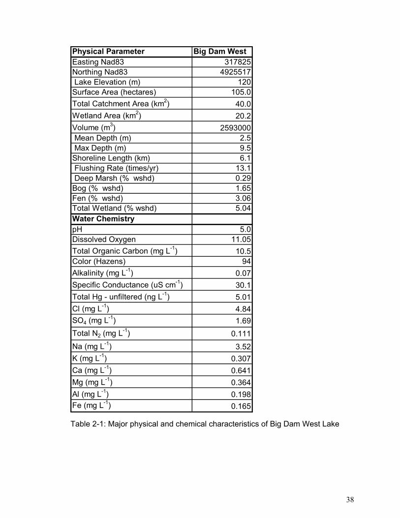
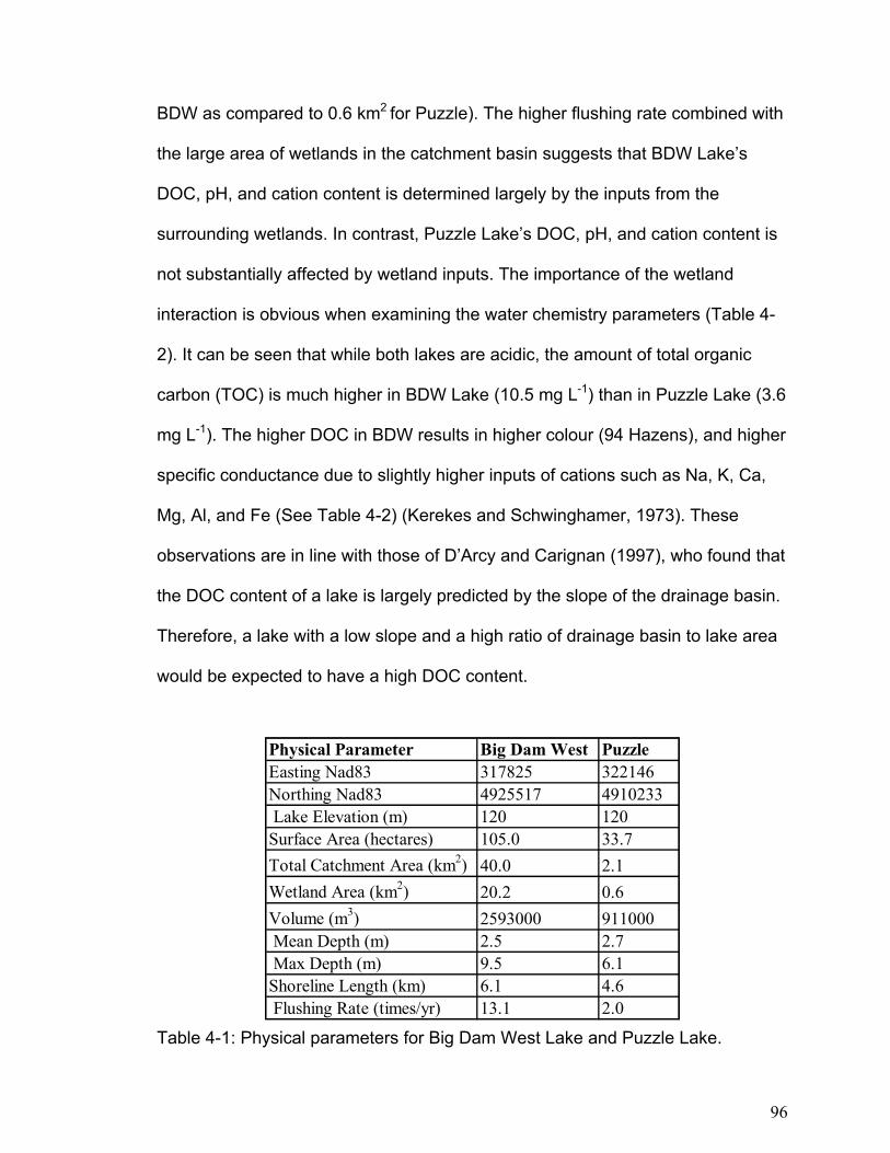
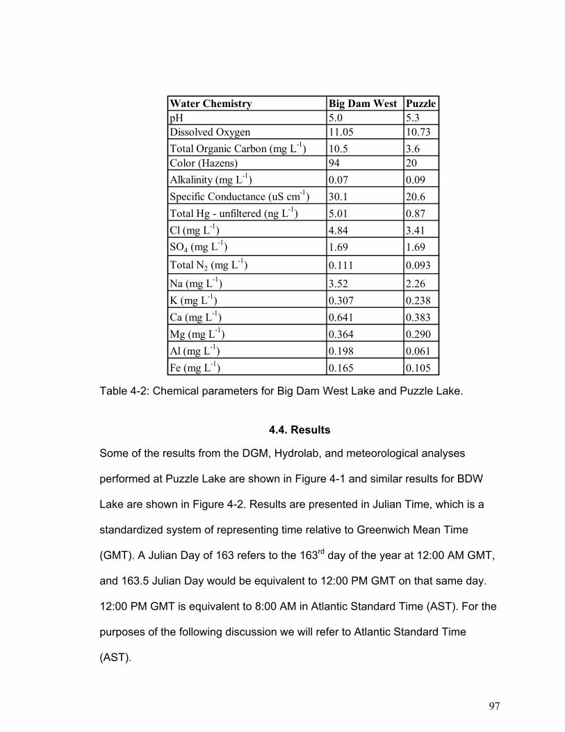
Table 2-1: Major physical and chemical characteristics of Big Dam West Lake
38
2.3 Methods
Various methods were used to obtain the data from different media presented in
this paper. The following is a summary of the major sampling and analytical
methods used to derive data for the presented mass balance.
2.3.1 Lakewater & Inflow/Outflow Sampling and Analysis
Water samples were collected from the major inlets (Thomas Meadow Brook,
Ford Brook, BDE inlet), outlets (Still Brook), and the center of the lake for total
mercury analysis. Total mercury samples were collected in 500 mL Teflon bottles.
The bottles were pre-cleaned in the laboratory through several stages: washing
with Contrad70 detergent / purified water, soaking for one week with reagent
grade HNO3, , followed by a purified water rinse, soaking for one more week with
Seastar high purity HNO3, final rinsing with copious amounts of polished high
purity water (>10 Mohms), and filling to the top with high purity water and stored
until use in individual Ziplock bags with a pair of latex surgical gloves for
manipulation of samples. After sampling the bottles were returned to the bags for
shipping.
Total mercury samples were digested in the presence of bromine monochloride
(BrCl) and UV irradiation. All samples were then pre-reduced with hydroxylamine
hydrochloride and reduced to elemental form with SnCl2. The Hg0 is purged from
39
the sample with nitrogen onto a gold-coated wire trap, and desorbed by heating
and purging the trap with a stream of argon into the atomic fluorescence detector
(CV-AFS). The method detection limit is 0.2 ng L-1.
2.3.2 Total Mercury in Precipitation
Precipitation samples used for mercury analysis were collected using an
Aerochem Metrics Model 301 automatic sensing wet/dry precipitation collector
with Teflon coated lid supports and gasket pads to prevent evaporative sample
loss. The sampler was equipped with a 128 cm sampling orifice and a borosilicate
glass sampling train leading to a 1 L borosilicate glass bottle housed in a
temperature controlled enclosure. The sampler was located at the CAPMON
research site near the entrance of Kejimkujik Park (~ 8km South East of BDW
Lake). Precipitation amounts were measured using a Belfort Model B-5-780
recording rain gauge results of which were confirmed by comparison with an
adjacent fixed mount standard rain gauge. The precipitation sample collection,
analysis and QA/QC were carried out according to protocols developed by the
National Atmospheric Deposition Program (NADP) Mercury Deposition Network
(MDN). Descriptions of instrumentation, sampling, analytical and QA/QC
protocols are contained in NADP (1996a, 1996b).
2.3.3. Groundwater Sampling
Groundwater samples were obtained from 11 piezometers and 4 seepage meters
40
installed near shore at 60 – 90 cm depth. A galvanized stainless steel pipe (6’
length; ¾″ i.d.) was driven into the near shore sediment and a LDPE tube (7’
length; ½ ″ o.d.) fitted with a piezometer tip was inserted into the steel pipe. The
piezometer tip consists of a LDPE tube (5’ length; ⅜” i.d.), with 1 cm holes and
wrapped with 0.25 mm Nitex (nylon monofilament) screening. The metal pipe was
slowly removed and the surrounding sediment compacted to ensure a good seal.
Ground water was collected using a hand pump in line with a 1000 mL glass
filtration flask connected to the LDPE tubing. Water was pumped prior to
sampling to reduce silt content. Fitting the tube with an opaque HDPE bag below
the water surface allowed for water collection over longer time spans (24 – 48
hours). After collection water samples were prepared for total mercury analysis
as outlined above. Steel cylindrical seepage meters (area of 1.07 m2) were
installed in close proximity to the piezometers. An opening in the cylinder top was
fitted with a rubber stopper connecting a HDPE tube and polypropylene reservoir
bag. The water was collected over a 12 - 24 hour period.
2.3.4. Soil-Air and Water-Air Flux
Air-surface mercury exchange was measured on BDW Lake and the surrounding
forested site using a rectangular Teflon flux chamber (Carpi & Lindberg, 1998)
placed over the substrate enclosing an open surface area of 0.12 m2 (Kim &
Lindberg, 1995; Carpi & Lindberg, 1997). Teflon sampling lines and fittings were
used throughout the mercury flux measurement system. Gaseous elemental
mercury (GEM) concentration in air was measured using a Tekran Model 2537A
41
CV-AFS calibrated using an internal mercury permeation source and an external
Tekran Model 2505 primary mercury vapor calibration system.
Unfiltered ambient air was sampled for 5 minutes alternating every 10 minutes
(duplicate 5 min integrated samples) between ambient and chamber air.
Switching between ambient and chamber air sampling was done using a Tekran
Model 1110 Synchronized Automated Dual Sampling (TADS) switching system.
To avoid stagnation of air in the system when samples were not being taken, air
was continuously drawn through the system using an air pump set to 1.5 L min-1.
Flow rates in the analysis system (1.5 to 10 L min-1) were controlled using
Hastings-Teledyne mass flow controllers and mass flow meters. Mercury flux
was calculated as the difference between the mercury concentrations in ambient
air versus air which had passed through the chamber (Schroeder et al., 1989 and
Xiao et al., 1991).
System quality control (QC) procedures including the use of standard operating
procedures (SOPs), analyzer and sensor calibrations, chamber/system blanks
and Hg injection-recovery tests were performed on a regular basis. Chamber
blanks were performed in the laboratory and in situ using the complete system
(lines, fittings, solenoid switches and the chamber). Flux rates presented in this
study are blank corrected.
2.3.5 Sediment
42
Sediment samples were obtained using an open-barrel coring system that is best
suited for sampling of soft-bottom sediments (Blomqvist, 1991; Stephenson et al.,
1996). Cores were obtained (July of 1999 and 2000) using a modified Kajak-
Brinkhurst (KB) gravity corer, fitted with 1-metre long polycarbonate tubes (i.d. 3”,
1/8 “wall). All cores (disturbed cores were discarded) were extruded and
sectioned immediately in the field using a aluminum extruding stand. Supernatant
water was siphoned off (to 5 cm water cover) prior to extrusion. Cores were
sectioned as follows: every 0.5 cm for first 10 cm, every 1-cm from 10-30 cm,
every 2 cm from 30-50 cm, and every 4 cm for depths greater than 50 cm. All
equipment was rinsed with distilled de-ionized (d.d.) water and Kimwipes
between samples. Sediment samples were collected in WhirlPak bags and kept
cold until analysis.
Two cores were used to determine the down core changes in water content and
bulk density using centrifugation and drying weights. Sediment samples were
freeze-dried and then ground to a homogenous powder in a class-100 clean
room using a mortar and pestle. The digestions were performed in a Questron
QLAB 6000 Microwave Digestion Oven. Very High Pressure (VHP) Teflon
digestion vessels were used to digest each 0.2 g of the dry, homogenized
sediment. The following pressure control program was used for 25 minutes: 600
W power, 200°C temperature limit, and 200 psi pressure limit. 5 mL of HNO3 and
2 mL of HF was added to the jar and digested to dryness. Once dry, 2 mL of
environmental grade 8 N HNO3 was added and digested to dryness again. This
43
step was repeated one more time and then 2.5 mL of environmental grade 8 N
HNO3 was added to the vessel and digested until all of the sample dissolved.
The contents of the jar were transferred to 125 mL HDPE container. The
digestate was diluted with MQ water to a final weight of 100 g.
Dating of the sediment deposits and determination of the sedimentation rates
were based on 210Pb and 137Cs methods, measured by γ-ray spectrometry at the
USGS Geochronology Laboratory in Denver, Colorado. Four cores were taken
from each lake and then the corresponding depth sections from each core were
combined in a WhirlPak bag as one sample. From these samples, 30 were
selected (15 from each lake) for freeze-drying and γ-ray spectrometry. Gamma-
ray spectrometry for the determination of 210Pb and 137Cs was done with a high-
purity Germanium well-type semiconductor of 16 mm diameter. From the activity
of 210Pbex and log 210Pbex vs depth plots, the age and sedimentation rates can be
determined. In attempt to verify the results of 210Pb dating, 137Cs was also
measured as an independent chronostratigraphic marker.
Mercury in sediment samples were analyzed by aqua-regia (3:1 HCl : HNO3, and
0.01% K2Cr2O7) digestion method. 5 mL of aqua-regia was slowly added to 0.1 g
of dry, homogenized sample in a pre-weighed 50 mL polypropylene Falcon
centrifuge tube and left to stand for at least 5 hours. After this time, the caps
were tightened and the vessels were shaken vigorously for about one minute.
The tubes were then placed in a hot water bath for 5 hours at 80°C, and then left
44
overnight to cool. The digested sample was then diluted to 50 mL with 0.01%
K2Cr2O7 in distilled de-ionized water, re-capped, and the final weight recorded.
The diluted digests were then shaken again for approximately one minute and
then centrifuged for 10 minutes at 3500 rpm. The digested samples were
analyzed by CV-AFS using a PS Analytical Millennium Merlin/Galahad mercury
analyzer.
Sedimentation rates of mercury were also obtained using sediment traps to
compare deposition with net accumulation. Four sediment traps collected sample
over an 11-month period (August 14, 2000 to July 12, 2001). An aluminium frame
(61 cm diagonal measurement) secured the traps in an upright position and
prevented substantial movements. The sediment chambers consisted of
polycarbonate plastic core tubes (10.2 cm diameter, 88 cm long) with 5 cm deep
ABS caps on the bottom. This provided an aspect ratio (depth/width) of 9.5 to
avoid sediment resuspension and loss during mixing events. The traps were
located in Big Dam West at 3.6 m at a water depth of 6.1 m using polyethylene
rope attached to a rock in the sediments and held in place using a subsurface
float. The samples were collected, frozen, and then freeze-dried. The amount (+/-
SD) for BDW was expressed on an areal basis by dividing by the area of the
traps (0.08023 m2) and correcting for 12 months to obtain annual sedimentation
rates. The rates in BDW were 45.58 +/- 3.34 mg m-2 y-1 (n = 4).
The interpretation of sediment trap data has been widely debated due to
problems of decomposition, sediment re-suspension, changing redox conditions,
45
predation by zooplankton and other invertebrates, and death and decay by these
opportunistic animals. Nevertheless, the data obtained provides some
confirmation of the lead isotope results. From the sediment trap data the mercury
sedimentation rate in BDW was found to be 91.2 µg m-2 y-1 or 95.73 g y-1. In this
study the lead isotope estimates of sedimentation have been used for all
calculations.
2.3.6 Vegetation
Samples of leaf and twig tissue from the dominant tree species were collected in
and around Kejimkujik Park. Dominant trees included: red maple (Acer rubrum),
white pine (Pinus strobus), eastern hemlock (Tsuga canadensis) and white birch
(Betula papyrifera). Duplicate samples were taken from adjacent trees at one in
every 10 sites, however not all species were present at each of the sites.
Samples were placed in paper bags, air-dried and returned to the lab for
chemical analyses (Rencz et al., 2003), along with control materials in order to
verify lab accuracy. Mercury concentrations were determined by the Milestone
Advance Mercury Analyzer (AMA-254).
In order to calculate the net uptake of mercury into vegetation surrounding Big
Dam West Lake average mercury concentrations were calculated for coniferous
and deciduous tree species. This was incorporated into a GIS analysis by
producing a look-up table in PCI (version 6.3) for average mercury for each of the
Canadian land classification units derived from remote sensing imagery. Using
46
the look up table and the land classification index layer for Kejimkujik Park, a new
GIS layer was created containing the average mercury concentrations in
vegetation (ng Hg g-1 plant tissue). Primary productivity was then used provide an
average net mercury in vegetation layer with units ng 25 m-2 y-1(this is, the
average mercury per 25 m-2 pixel block). Average net mercury in vegetation was
then calculated for the Big Dam West Lake basin and multiplied by the terrestrial
area in the basin to obtain the average net mass of mercury incorporated into the
vegetation within the Big Dam West lake basin.
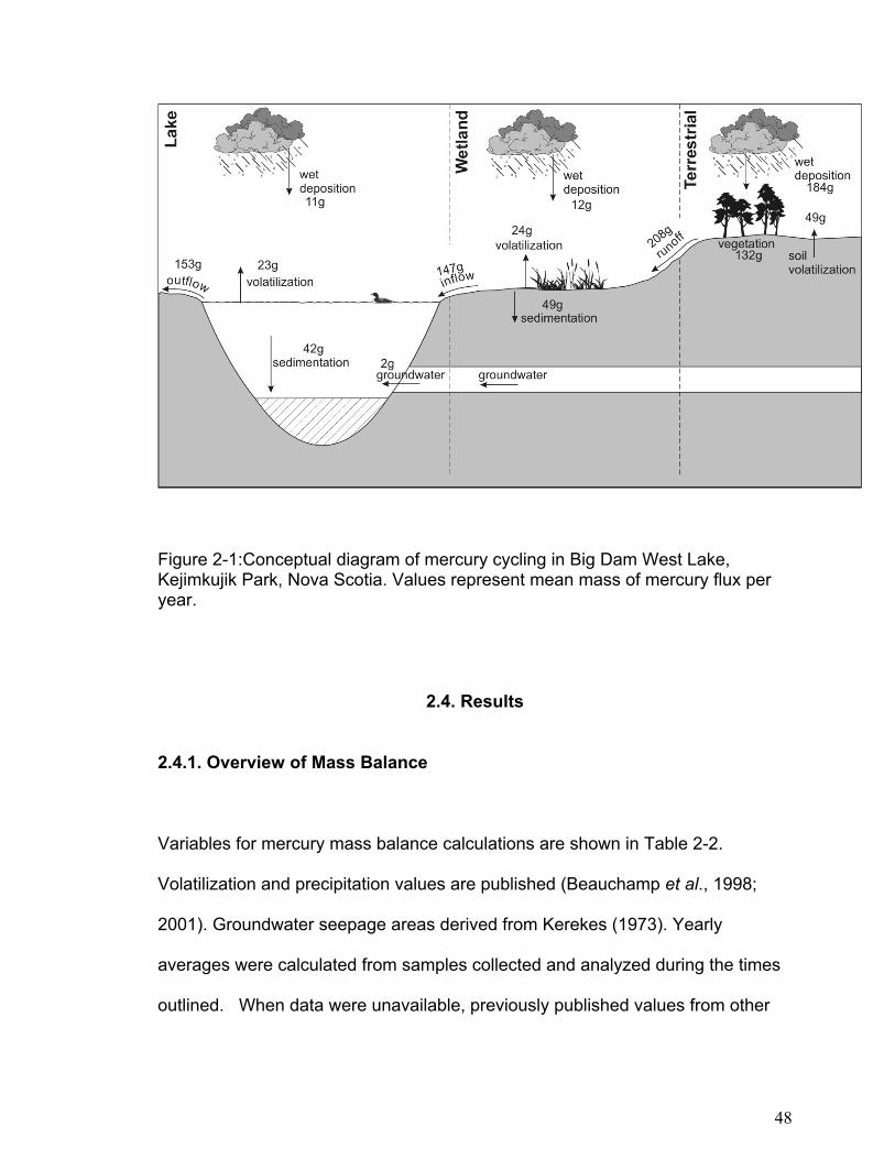
2.3.7. Mercury Conceptual Model
Figure 2-1 is a conceptual model of mercury movements in BDW watershed. The
watershed was divided into 3 units based on the Canadian Land Classification
Index and remote sensing data. Lake represents only the area covered by the
lake surface, wetland is classified as areas that have standing water with
vegetation, and the terrestrial portion as dry land that is covered by vegetation.
These areas were calculated using remote sensing data.
47
Figure 2-1:Conceptual diagram of mercury cycling in Big Dam West Lake, Kejimkujik Park, Nova Scotia. Values represent mean mass of mercury flux per year.
2.4. Results
2.4.1. Overview of Mass Balance
Variables for mercury mass balance calculations are shown in Table 2-2.
Volatilization and precipitation values are published (Beauchamp et al., 1998;
2001). Groundwater seepage areas derived from Kerekes (1973). Yearly
averages were calculated from samples collected and analyzed during the times
outlined. When data were unavailable, previously published values from other
48
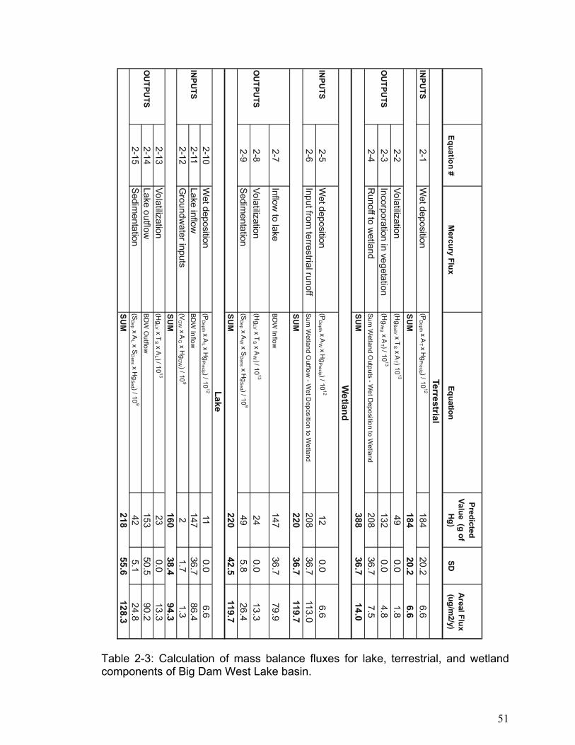
studies were used. Watersheds were divided into 3 distinct units for examination
of mercury flux based on the conceptual model shown in Figure 2-1. This model
was thought appropriate since inflows from wetlands are the primary source of
water flow in Big Dam West Lake, and negligible amounts of water inputs are due
to direct runoff (as suggested by water balances of inflow and outflow budgets)
(Clair et al., In Press). Mass movement of mercury within and between these
units was calculated using the equations outlined in Table 2-3.
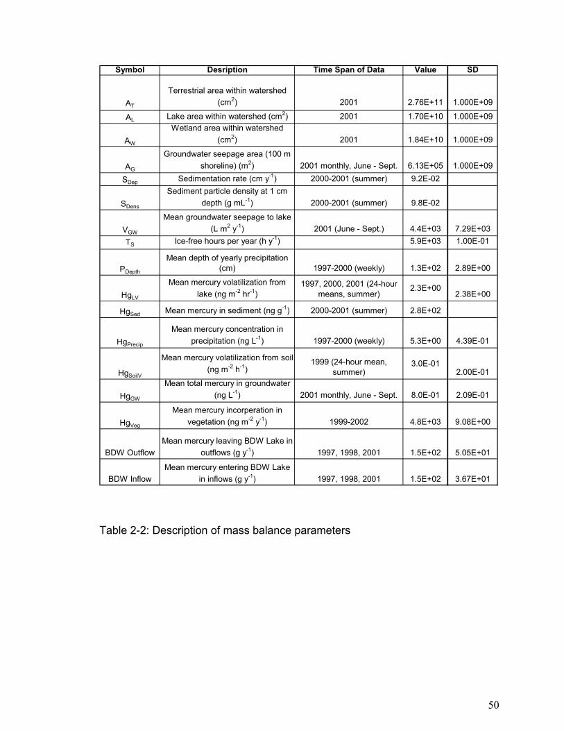
The ecosystem data, estimated uncertainty, data source and time span are
shown in Table 2-2, while the calculations and results used to populate the
conceptual model are displayed in Table 2-3. When possible precision was
expressed as one standard deviation.
49
Symbol Desription Time Span of Data Value SD
AT
Terrestrial area within watershed (cm2) 2001 2.76E+11 1.000E+09
AL Lake area within watershed (cm2) 2001 1.70E+10 1.000E+09
AW
Wetland area within watershed (cm2) 2001 1.84E+10 1.000E+09
AG
Groundwater seepage area (100 m shoreline) (m2) 2001 monthly, June - Sept. 6.13E+05 1.000E+09
in inflows (g y-1) 1997, 1998, 2001 1.5E+02 3.67E+01
Table 2-2: Description of mass balance parameters
50
Table 2-3: Calculation of mass balance fluxes for lake, terrestrial, and wetland components of Big Dam West Lake basin.
Equation #M
ercury FluxEquation
Predicted Value (g of
Hg)
SDA
real Flux (ug/m
2/y)
Terrestrial IN
PUTS
2-1W
et deposition(P
Depth x A
T x Hg
Precip ) / 1012
18420.2
6.6
SU
M184
20.26.6
2-2Volatilization
(Hg
SoilV x TS x A
T ) 1013
490.0
1.8O
UTPU
TS2-3
Incorporation in vegetation(H
gVeg x A
T ) / 1013
1320.0
4.82-4
Runoff to w
etlandSum
Wetland O
utputs - Wet D
eposition to Wetland
20836.7
7.5
SUM
388
36.714.0
Wetland
INPU
TS2-5
Wet deposition
(PD
epth x AW
x Hg
Precip ) / 1012
120.0
6.62-6
Input from terrestrial runoff
Sum W
etland Outflow
- Wet D
eposition to Wetland
20836.7
113.0
SU
M
22036.7
119.7
2-7Inflow
to lakeBD
W Inflow
14736.7
79.9
OU
TPUTS
2-8Volatilization
(Hg
LV x TS x A
W ) / 1013
240.0
13.32-9
Sedimentation
(SD
ep x AW x S
Dens x H
gS
ed ) / 109
495.8
26.4SU
M220
42.5119.7
Lake 2-10
Wet deposition
(PD
epth x AL x H
gPrecip ) / 10
1211
0.06.6
INPU
TS2-11
Lake inflowBD
W Inflow
14736.7
86.42-12
Groundw
ater inputs(V
GW x A
G x Hg
GW ) / 10
92
1.71.3
SU
M160
38.494.3
2-13Volatilization
(Hg
LV x TS x A
L ) / 1013
230.0
13.3O
UTPU
TS2-14
Lake outflowBD
W O
utflow153
50.590.2
2-15Sedim
entation(S
Dep x A
L x SD
ens x Hg
Sed ) / 10
942
5.124.8
SU
M218
55.6128.3
51
2.4.2. Calculation of Uncertainty
The standard deviation for each flux calculation was calculated as consistently as
possible given that the data was collected at different times and over different
time scales. It should also be noted that calculated deviations are only
methodological and sample analysis related and do not reflect all sources of
environmental variations. In cases where too little data was available to assess
sample variations, method detection limits were used for standard deviation (e.g.
number of ice free hours, area calculations from remote sensing, etc).
The lake inlet and outlet numbers are calculated as the mean of samples
collected over the years 1997, 1998, and 2001. If we calculate the standard
deviation as the deviation between yearly means (with each yearly mean derived
from 26 measurements), this results in a % RSD of 25 and 33 % for inflows and
outflows respectively. Therefore differences observed between inflows and
outflows are insignificant. It is likely that the calculated mean does not accurately
represent the long-term yearly average due to the small sample size, and the
above calculations of error are very rough estimates.
Variation between lake water flux numbers were calculated as the variation
between the means of three 24-hour readings taken over BDW water in the
summers of 1997, 2000, 2001. No variation is available for undisturbed forest soil
as only one 24-hour mean was measured in the summer of 1999. Therefore, a
52
value for mean positive flux method detection limit was used (3X standard
deviation of blank).
Detailed descriptions of sediment lead isotope calculations are available from
Telmer and DesJardins (In Press). Variation for precipitation was taken from
values of mean precipitation amounts measured weekly for the years 1997 -
2000. Similar variations were calculated for volume weighted mean
concentrations of mercury in precipitation. These flux values were scaled up to a
yearly flux value assuming that no significant flux occurs during the periods of ice
and snow cover (December – March Inclusive).
2.5. Discussion
2.5.1. Comparison of Flux Values to Literature
The results obtained for mercury fluxes are consistent with the published
literature. The mean water-to-air volatilization observed on Big Dam West Lake
(2.3 ng m-2 h-1, σ = 2.38) is less than what has been observed in contaminated
wetland systems (mean = 43 ng m-2 h-1, σ = 5) (Wallschlager et al. 2002).
However, it is similar to readings over Lake Ontario and the upper St. Lawrence
River (median = 1.85 and 1.76 ng m-2 h-1 respectively) using the gradient
technique for flux measurement (Poissant et al. 2000). The mean soil-to-air
volatilization (0.3 ng m-2 h-1, σ = 0.20) was similar to Xiao et al. (1991) who (using
53
a stainless steel flux chamber) observed mercury fluxes ranging from –2 to 2 ng
m-2 h-1 over uncontaminated forest soils.
The mean mercury in precipitation value of 5.3 ng L-1 (σ = 0.439 between annual
means) observed in this study falls towards the lower end of the 5 – 100 ng L-1
range observed by several researchers (Lee and Iverfeldt, 1991; Pleijel and
Munthe, 1995; US EPA, 1997, St. Louis et al., 2001). The mercury in ground
water observed in this study (0.80 ng L-1, σ = 0.209) is similar to that found by
Krabbenhoft and Barbiarz (1992) (2-4 ng L-1). Krabbenhoft and Barbiarz (1992)
also observed mercury inputs of 0.7 g y-1 to Pallete Lake, Wisconsin; which is
similar to the 2.0 g y-1 (σ = 1.7) calculated for Big Dam West Lake in this study.
2.5.2. Relative Magnitude of Fluxes
Wet precipitation was the only source of mercury considered to the terrestrial
system accounting for 184 (σ = 20.2) g of mercury deposited. The total outputs
from the terrestrial system accounted for 388 g (σ = 36.7), of that, 34% (132 g, σ
= 0.0) was incorporated into vegetation and, 13% (49 g, σ = 0.0) was volatilized
from the soil surface. Although were unable to measure mercury runoff directly,
208 g would be necessary in order to balance the inputs and outputs of the
wetland component. While this value is not significantly larger than what falls in
wet deposition (given the error on the mean values), a larger output value might
indicate mercury transport associated with soil erosion.
54
It should be emphasized that the source of mercury to vegetation and terrestrial
runoff is unclear and is not necessarily wet precipitation. Direct atmospheric
uptake and root uptake of mercury are possible mechanisms that were not
accounted for in this budget. Therefore the imbalance of terrestrial inflows and
outflows that results from this calculation would be improved with data for root to
vegetation flux measurements. Runoff was the only flux in the mass balance that
has been calculated by the difference of other inputs and outputs.
Of the mean 220 g (σ = 36.7) of mercury inputs to wetlands, 95% (208 g, σ =
36.7) was due to terrestrial runoff and 5% (12 g, σ = 0.0) was due to wet
deposition. The total outputs from the wetland accounted for 220 g (σ = 36.7),
67% (147 g, σ = 36.7) was removed by outflow to the lake, 22% (49 g, σ = 3.6)
was deposited to sediment and, 11% (24 g, σ = 0.0) was volatilized from the
wetland surface.
Of the mean 160 g (σ = 38.4) of mercury inputs directly to the lake, 92% (147 g, σ
= 36.7) was due to inflow from wetlands, 7% (11 g, σ = 0.0) was due to wet
precipitation and, 1% (2 g, σ = 1.7) was due to groundwater inflow. The total
outputs from the lake accounted for 218 g, 70% (153 g, σ = 50.5) was removed
by outflow, 19% (42 g, σ = 3.6) was deposited to sediments and, 11% (23 g, σ =
0.0) was volatilized from the lake surface. It should be noted that total outputs
were larger than inputs by 58 g (see section 13.5.4.), however this is not
significant in light of the deviation observed in these values.
55
Henry et al. (1995) performed a mass balance on Onondaga Lake, NY and found
that total mercury inputs accounted for 14.116 kg. Of the total inputs, 96.3%
(13.6 kg) was due to terrestrial inflows, 3.1% (0.44 kg) was atmospheric
deposition, 0.4% (0.056 kg) was sediment flux and, 0.1% (0.02 kg) was
groundwater. Of the 13.916 kg of outputs, sedimentation accounted for 79.8%
(11.1 kg), outflow 20.1% (2.8 kg), and volatilization 0.1% (0.016 Kg). These
results compare well with what was observed in this study with inflows
contributing the majority of the total mercury, followed by precipitation and
groundwater. However, the outputs of the two lakes are quite different. Outflow is
the primary sink in BDW Lake, whereas sedimentation is the dominant sink in
Onondaga Lake. The lakes are in fact opposite in terms of outflow versus
sedimentation. The level of volatilization is substantially higher in BDW as
opposed to Onondaga Lake (11% and 0.1 % respectively) (See Figure 2-1)
2.5.3. The Role of Wet Deposition in Volatilization
The area within the BDW drainage basin is largely dominated by the terrestrial
ecosystem. Of the 31.18 km2 in the BDW watershed 88.7 % is terrestrial, 5.9 % is
wetland, and 5.5 % is lake surface. The 207 g of mercury deposited in
precipitation follows a similar distribution. Of the 96 g of mercury volatilized from
all surfaces in the BDW watershed 51% is from the terrestrial soil, 26% is from
the wetlands, and 24% is from the lake surface. In this context, it may appear that
soil volatilization is the most important mercury removal process, however the
percentage of volatilization relative to the amount of direct wet deposition within
56
the terrestrial, wetland and lake compartments is 27%, 200%, and 200%
respectively. The high amounts of mercury volatilization relative to wet
precipitation indicate that volatilization is an important process within this
ecosystem, particularly over water (double the direct wet deposition). Over the
entire basin area the mass of mercury volatilized is 46% of the mass deposited
by wet deposition. It is likely that a combination of several factors limit mercury
volatilization. Some limiting factors might include the availability of photo-
reducible mercury in wet deposition, wind speed, or amounts of cumulative solar
radiation.
Several researchers have found that levels of DGM formation and mercury
volatilization from lake surfaces are linked to rainfall events. Vandal et al. (1994)
observed that that the influx of reactive mercury in wet deposition may account
for a large portion of elemental mercury production in Pallette Lake Wisconsin,
USA. Similarly soil moisture contents have been linked to precipitation and
volatilization. Johnson and Lindberg (1995) found that elemental mercury
concentrations in soil increased exponentially with moisture content.
2.5.4. Sources of Error
The inputs and outputs of the lake component are close to being in balance,
while the terrestrial is substantially out of balance (184 g inputs and 388 g
outputs). The reason for the imbalance may be due either to error in
measurements that were not accounted for, or due to missing inputs or outputs.
57
There are several possible fluxes of mercury that have not been adequately
accounted for in this study. We were unable to account for mercury volatilization
or scavenging by the forest canopy. The forest canopy has been found by many
researchers to have dynamic exchanges with the atmosphere (St. Louis et al,
2001; Leonard et al., 1998a; Leonard et al., 1998b). St. Louis et al. (2001) found
that through fall volumes at boreal ecosystem sites ranged between 43 - 69 % of
the direct wet deposition, due to canopy interception and evapotranspiration.
Litter fall is another source of mercury within the terrestrial system that has not
been accounted for in this mass balance. Grigal (2002) estimates that deposition
to lake surfaces is only about one fourth the deposition to forests by through fall
and litter fall combined. We were also not able to account for mercury uptake by
tree roots. We were also unable to measure any interaction between geology and
mercury movement into runoff. An average value for mercury in the soil Ah
horizon (silt size fraction) surrounding BDW lake is 466 ng g-1 (Rencz et al.,
2003). Since there is a large pool of mercury stored in soil and geology, any
mobilization of this pool would affect our interpretation of mass movements.
Mobilization of mercury from the sediment storage pool was also not measured in
this study and may constitute an important input to lake mercury levels. In
addition, since no sediment sampling was performed for the wetland area of the
catchment, the rate of sedimentation in the wetland portion of the mass balance
was assumed to be equal to the lake portion of the catchment. This is likely a
very rough estimate.
58
The importance of mercury dry deposition and reactive gaseous mercury
deposition was not examined in this mass balance. This is an emerging area of
research with the new analysis technology currently being assessed and tested.
However we acknowledge that these unaccounted inputs may in part explain the
imbalances observed. Future research may shed some light on the magnitude of
these inputs.
2.5.5. Summary
In summary, volatilization of mercury was found to be an important process in the
Big Dam West Lake catchment. The magnitude of volatilization appears to be
approximately double the direct wet deposition over the lake and wetland areas,
and 27% of the direct wet deposition to the terrestrial area of the catchment. Over
the entire basin area the mass of mercury volatilized is 46% of the mass
deposited by wet deposition. In addition, it was observed that the terrestrial
catchment dominates the processes occurring in the BDW watershed. Terrestrial
vegetation was found to play a significant role in mercury movement as
evidenced by the large amount of mercury uptake found in this study (132g). The
importance of terrestrial vegetation is not fully explored since 3 important mercury
fluxes were not measured: (i) uptake from roots, (ii) volatilization from leaves, and
(iii) litter fall.
59
Chapter 3
CONTINUOUS ANALYSIS OF DISSOLVED GASEOUS MERCURY
IN FRESHWATER LAKES
Reproduced in part with permission from: O’Driscoll, N.J., Siciliano, S., and Lean, D.R.S. 2003. Continuous analysis of dissolved gaseous mercury in freshwater ecosystems. Science of the Total Environment. 304(1-3): 285-294. Copyright (2003) Elsevier Press.
60
3.1. Abstract
The concentration of dissolved gaseous mercury (DGM) in freshwaters changes
more quickly than the 40-minute processing time of current analytical methods. A
new method for continuous field analysis of DGM was developed using a Tekran
2537A to achieve a DGM analysis time of 5 minutes. Samples are concurrently
analyzed for temperature, oxygen, conductivity, pH, and oxidation-reduction
potential using a Hydrolab. The method detection limit for DGM was 22.4 fmol L-1
with 99% removal efficiency. Control experiments showed that there was no
interference due to methyl mercury (MeHg), which is present in similar
concentrations to DGM. Controlled experiments comparing continuous DGM
analysis with discrete DGM analysis showed that the results are not significantly
affected by typical variations in water temperature (4- 30 o C), oxidation-reduction
Figure 3-5: Difference between continuous and the discrete dissolved gaseous mercury (DGM) analyses with varying dissolved organic carbon (DOC) concentrations.
74
0
1000
2000
3000
0 1000 2000 3000
Discrete Values (fmol L-1)
Con
tinuo
us V
alues
(fm
ol L
-1) y = 1.045 x + 6.7
Figure 3-6: Scattergram of discrete versus continuous measurements.
The theoretical method detection limit (given that the detection limit of the Tekran
2357A is 1 pg of elemental mercury) for continuous analysis would be 20 fmol L-1.
The precision of the analysis system as determined as the average percentage
relative standard deviation on a replicated sample was found to be 4.0 +/- 2.6%
(n=36) giving an operational detection limit of 22.4 fmol L-1. In order to test
interference by MeHg in the analysis of elemental mercury, 4638 fmol of methyl
mercury chloride was added to a 1 L water sample and analyzed in discrete
sample mode and only 27.9 fmol DGM was detected or 0.6% of the methyl
mercury spike. This suggests that for a typical environment containing 500 fmol L-
1 MeHg, only 3 fmol or 0.75% of the DGM signal (using a typical DGM value of
400 fmol L-1) would be due to MeHg. While more testing is needed to determine
DGM speciation, it is likely that the predominant form of mercury measured is
75
elemental.
Some of the results of the DGM and Hydrolab analyses performed at Big Dam
West Lake are shown in Figures 3-7 and 3-8 respectively (similar data was
collected for Puzzle Lake). Both lakes showed smooth changes in DGM, pH,
ORP, and water temperature, (indicating reproducible readings in these
parameters). The accuracy of the pH, ORP, and temperature probes used in the
Hydrolab are +/- 0.2 pH units, +/- 1 mV, and +/- 0.1 oC respectively (Hydrolab,
1997). Over 1000 data points for each parameter was successfully collected over
the two 48-hour testing periods with a loss of less than 1% of the data due to a
power failure.
3.5. Discussion
DGM analysis has been the subject of many other research papers, however, it is
still unclear what DGM actually is. Elemental mercury has been suggested by
other researchers to be the primary constituent of DGM due to its high Henry’s
law constant and presence in the atmosphere (Schroeder et al., 1991, Vandel et
al., 1991). We have demonstrated in this study that methyl mercury does not
interfere with DGM analysis, but it is unknown if the same is true for other volatile
mercury species.
76
0
200
400
600
800
1000
12:0
018
:00
0:00
6:00
12:0
018
:00
0:00
6:00
12:0
018
:00
0:00
Atlantic Standard Time
DG
M (f
mol
L-1
)
Figure 3-7: DGM measured in Big Dam West Lake on June 6-8, 2001 using the continuous analysis method for 48 hours
270
290
310
330
350
370
390
12:0
018
:00
0:00
6:00
12:0
018
:00
0:00
6:00
12:0
018
:00
0:00
Atlantic Standard Time
OR
P (m
V)
Figure 3-8: Oxidation Reduction Potential (ORP) measured in Big Dam West Lake on June 6-8, 2001 using the continuous analysis method for 48 hours
77
Most of the recently published papers on DGM analysis indicate a sample
sparging time ranging from 20 to 90 minutes, which leads to very poor temporal
resolution of DGM values (Krabbenhoft et al., 1998; Bayens and Leermakers,
1998; Amyot et al., 2000). This method gives a temporal resolution of 5 minutes,
which allows for a detailed investigation of relationships between water chemistry
and other variables that may affect DGM very quickly. Some of the sharp peaks
observed in the diurnal studies indicate that very quick changes are occurring in
the water concentration of DGM. Therefore fast processes are controlling both
DGM production and loss in the water column. Past research has assumed that
only discrete sample analysis could account for the difficulty in obtaining high
DGM extraction efficiency with time. This method overcomes that problem by
using a large volume sparger with a relatively slow water circulation rate (50 mL
min-1). The lag time for sample transport from the lake to the analysis system was
approximately 3 minutes at this speed.
If the water entering the sparger is thought of in discrete packets, then every 5
minutes 250 mL of lake water is introduced to the 1 L sparger. Therefore average
turnover time for water in the sparger is 20 minutes which is the amount of
bubbling time required to remove 99% of the DGM from an isolated water sample
as shown in Figure 3-1. The 20-minute bubbling time has also been shown by
other researchers to remove the majority of the dissolved gaseous mercury in
water (Amyot et al, 2000, Lindberg et al., 2000). The other advantage of this
sampling method is that there is no possibility of contamination during sampling
from external sources, and changes in sample composition are minimized due to
78
the extremely quick processing time. During the field trials, the Teflon lines were
run from the platform (at an approximate depth of 2 feet underwater) to an
analysis tent located on the lakeshore to minimize interaction with solar radiation.
We estimate that only 7.6% of incident solar radiation is available at this depth,
therefore the effects of photoreduction would be minimal during the 3-minute
sample tube residence time.
Since DGM extraction is temperature dependent (Figure 3-2) not all of the DGM
in the 5-minute sampling is extracted during that time. Since there is some carry-
over of DGM from one 5-minute sparging to the next we decided to give the
sparger a 20-minute residence time. Therefore all DGM is removed from water
entering the sparger during its 20-minute residence time. It is noted that there will
be some carry-over of DGM between each 5-minute data point (that will be most
noticeable at low temperatures). However at water temperatures ~20 oC, each
sampling point can be considered a composite value (i.e. approximately 80% of
the current 5 minute sample plus 15% of the previous five minute sample, etc..).
This gives the advantage of being able to observe sharp changes in DGM
concentration every 5 minutes while avoiding the underestimation and
temperature sensitivity of a 5-minute sparger residence time.
While calibration of analysis instrumentation has been a problem in previous
DGM studies due to a lack of obtainable or stable standard reference materials
for DGM, the Tekran 2357A mercury analyzer contains an internal elemental
mercury calibration standard for the measurement of mercury in air. The Tekran
79
is calibrated both to this standard and to standard injections of gaseous
elemental mercury in air to check the calibration source. While no liquid
calibration samples were analyzed (due to the unavailability of a suitable stable
standard for DGM) it was assumed that all volatile mercury is removed from the
sample within the analysis time. This was checked by re-sparging a sparged
sample and finding little DGM. Since 1 L of analysis air per minute is passed
through the sparger it is a safe assumption that the removal efficiency is high.
The removal efficiency is also aided by the sparger design, which is tall and thin
to allow for maximum sample interaction with the analysis air.
The close relationship between near-continuous and discrete measurements over
a range of pH, DOC, and temperature conditions indicates that the near-
continuous method gives consistent results within 4.5%. It is likely that this is just
due to analytical error that is involved with any chemical analysis. Sources of this
error may include changes in sample flow during the analysis or changes in redox
conditions during sample bubbling.
An example of the data collected for Big Dam West Lake is shown in Figures 3-7
and 3-8. The sharp peaks observed in DGM readings indicate the necessity of
having a fine time resolution for diurnal DGM data. Diurnal cycles were obvious in
both lakes for DGM and many Hydrolab parameters (ORP shown in Figure 3-8).
Recent research has identified a number of processes that can influence the
levels of DGM in lake water. The balance between photoreduction and
photooxidation processes (initiated by solar radiation principally in the UVA and
80
UVB spectrum) has been identified as important determinants of DGM
concentrations (Amyot et al., 1994). More recently, the role of microbial oxidation
and reduction processes in DGM diurnal cycles has been identified (Siciliano et
al., 2002). The Hydrolab parameters that were measured may also have an effect
on DGM production and volatilization, however they have not been previously
examined in detail over a diurnal cycle. Redox processes and reaction rates are
intimately linked to water temperature, pH, and ORP measurements in lake
water. A detailed examination of the data collected at both lakes is available in
Chapter 4.
In conclusion this method has been thoroughly tested and found to provide
consistent results when compared with the discrete analysis method. This
method has been determined to have a low detection limit, high accuracy and
precision, and a much reduced sample analysis time as compared with discrete
sample analysis. The automated system was tested at two remote freshwater
lakes and was found to collect 99% of the data (over 1200 data points) during two
48-hour periods. Applications of this method may include the examination of
quick ecosystem processes that alter DGM concentrations in water or real time
surveying of water chemistry both spatially and with depth in the water column.
81
Chapter 4
CONTINUOUS ANALYSIS OF DISSOLVED GASEOUS MERCURY
(DGM) AND MERCURY FLUX IN TWO FRESHWATER LAKES IN
KEJIMKUJIK PARK, NOVA SCOTIA: EVALUATING MERCURY
FLUX MODELS WITH QUANTITATIVE DATA
Reproduced in part with permission from: O’Driscoll, N.J., Beauchamp, S., Siciliano, S.D., Lean, D.R.S., and Rencz, A.N. 2003. Continuous analysis of dissolved gaseous mercury (DGM) and mercury flux in two freshwater lakes in Kejimkujik Park, Nova Scotia: Examining flux models with quantitative data. Environmental Science and Technology. 37(10): 2226-2235. Copyright (2003) American Chemical Society.
82
4.1. Abstract
Diurnal patterns for dissolved gaseous mercury (DGM) concentration, mercury
flux, several water variables (pH, oxidation reduction potential (ORP), water
temperature), and meteorological variables (wind speed, air temperature, %
relative humidity, solar radiation) were measured in two lakes with contrasting
dissolved organic carbon (DOC) concentrations in Kejimkujik Park, Nova Scotia.
A continuous analysis system made it possible to measure quick changes in
DGM over time. Consistently higher DGM concentrations were found in the high
DOC lake as compared to the low DOC lake. An examination of current mercury
flux models using this quantitative data indicated some good correlations
between the data and predicted flux (r ranging from 0.27 to 0.83) but generally
poor fit (standard deviation of residuals ranging from 0.97 to 3.38). Cross-
correlation analysis indicated that DGM dynamics changed in response to solar
radiation with lag-times of 65 and 90 minutes. This relationship with solar
radiation was used to develop new predictive models of DGM and mercury flux
dynamics for each lake. We suggest that a generalized approach using time-
shifted solar radiation data to predict DGM can be incorporated into existing
mercury flux models. It is clear from the work presented that DOC and wind
speed may also play important roles in DGM and mercury flux dynamics, and
these roles have not been adequately accounted for in current predictive models.
83
4.2. Introduction
Dissolved gaseous mercury (DGM), which is composed primarily of elemental
mercury, can volatilize from a lake’s surface to the atmosphere thus reducing the
amount of total mercury present (Baeyens et al., 1991; Vandal et al., 1991;
Amyot et al., 1997a). There is a positive correlation between the total amount of
mercury in freshwater lakes and the amount of methyl mercury (MeHg) present
during summer months (Driscoll et al., 1994; Watras et al., 1995; O’Driscoll et al.,
2001). Thus, predictive models of DGM flux to the atmosphere would help identify
ecosystems likely to retain more total mercury and accumulate MeHg, which is
the form of mercury that will bioaccumulate in aquatic food webs (Morel et
al.,1998).
There are significant changes in DGM over a diurnal cycle for both freshwater
and seawater systems (Amyot et al., 1994; 1997c; Lanzillotta and Ferrara, 2001).
These changes are the result of several oxidation and reduction processes
occurring simultaneously. Supporting the early work of Amyot et al. (1994),
Zhang & Lindberg (2001) found that iron-mediated photo-reduction and photo-
oxidation processes play a role in DGM dynamics. In addition to these chemical
processes, photo-induced microbial reduction and oxidation processes also
contribute to DGM dynamics (Siciliano et al., 2002).
In addition to studies of DGM, several recent publications have examined
mercury flux between water and air. Loux (2000) found that temperature effects
84
on chemical properties such as Henry’s law constants, and diffusive layer
properties may explain up to 44 % of diurnal mercury flux variations. Zhang and
Lindberg (2000) produced a box model of DGM evasion rates based primarily on
solar radiation and dissolved reactive mercury availability. All of the current
research indicates that solar radiation is directly or indirectly the driving force
behind diurnal variations in DGM and mercury flux.
Researchers often use predictive models to estimate mercury flux given a known
DGM concentration (Baeyens et al., 1991; Schroeder et al., 1992). Most of the
current mercury flux models are based on modified measurements of carbon
dioxide water-to-air transport (Schroeder et al., 1992; Poissant et al., 2000).
Some authors have also attempted to incorporate wind parameters into these flux
models based on theoretical calculations involving changes to the diffusive layer.
Current flux models have not been rigorously tested using large datasets of
quantitative field measurements due to significant challenges associated with
DGM analysis in lake water (as outlined in Chapter 3). Our group recently
developed and calibrated (under a wide range of DOC, pH, and water
temperatures) a continuous analysis system capable of measuring DGM and
Hydrolab readings (ORP, water temperature, pH, specific conductivity, dissolved
oxygen) every 5 minutes (O’Driscoll et al., 2003a). An alternative continuous
DGM analysis system was independently and simultaneously developed by
Amyot et al. (2001).
Several researchers (Schroeder et al., 1992; Boudala et al., 2000; Poissant et al.,
85
2000) have investigated spatial and temporal trends in mercury flux over water
using various chamber and micrometeorological designs. While it is recognized
that mercury movement between water and air is an important part of the
mercury cycle, only a few papers have measured DGM and mercury volatilization
at the same time, and none have done so continuously to examine diurnal
patterns (Poissant et al., 2000). The purpose of this paper was to examine diurnal
patterns in DGM and mercury flux continuously in two lakes with contrasting DOC
contents, and then use this data to evaluate current predictive models for
mercury flux from water.
4.3. Methods
4.3.1. Continuous analysis of DGM
Water was sampled from each lake site using ¼ inch diameter Teflon tubing that
had been pre-cleaned by passing 5 L of 5% HCl through it, followed by large
amounts (~20 L) of distilled de-ionized water. The Teflon tubing was also rinsed
with 5-10 L of the lake water being sampled, prior to starting the sampling
system. The sample inlet was fixed 10-15 cm below a floating Teflon platform that
was located approximately 15 meters from shore. The sample depth was chosen
to give a representation of near-surface water while avoiding flux chamber
interferences and air sampling during high wave conditions. The Teflon tubing
was 60 cm below the surface of the water until it reached the shore and then was
exposed to sunlight over a 1 m interval between the tent and shoreline. A solar
86
radiation extinction coefficient of 4.6 m-1 was calculated by extrapolating the
dependence of two-year (1979-1981) extinction coefficients for Beaverskin,
Kejimkujik and Pebbleloggitch Lakes on colour (Hazen units, r2 = 0.979) to Big
Dam West Lake (Hazen unit = 94) (Beauchamp et al.,1989). Thus the tubing was
exposed to only 7.6% of the surface incident radiation (3.8% of total radiation) for
a total of 3 minutes while in transport to the analyzer (Environment Canada,
1982). A detailed description of the analysis system is available in Chapter 3.
When in continuous mode, water was pumped (using a two channel peristaltic
pump with silicone pump tubing) from the lake to the Hydrolab for analysis of
water chemistry (Hydrolab, 1997), and then to the bottom of a 1 L graduated
glass sparger. Water was then pumped from the sparger at the 1 L volume mark
back to the lakeshore. With a flow rate of 50 mL min-1 the volume of sample
analysed was 250 mL every 5 minutes. This flow rate and sparge time has been
shown to be comparable with previous discrete analysis methods (O’Driscoll et
al., 2003a). A Tekran 1100 zero air generator was used to supply mercury-free
air to the glass sparger at a rate of 1.0 L min-1. The mercury-free air bubbled the
sample through a coarse glass dispersion tube that was placed at the bottom of
the glass sparger close to the lake water inlet. The DGM is carried from the
sparger to the sample inlet of the Tekran 2537A and analyzed for mercury
content. Each Tekran 2537A used for this study was calibrated prior to this
analysis using the internal mercury permeation calibration source. The internal
mercury calibration source was checked for accuracy with a standard air injection
87
of elemental mercury using a Hamilton digital syringe and a Tekran 2505
mercury vapour calibration unit. The analysis system was allowed to warm up
and stabilize for a minimum of 2 hours before readings were recorded for
interpretation. Using this method the detection limit for DGM was 20 fmol L-1 and
the relative standard deviation (RSD) of duplicates (n=36) was 4.0 +/- 2.6 %
(O’Driscoll et al., 2003b).
4.3.2. Continuous Analysis of Gaseous Elemental Mercury in Ambient Air
Gaseous elemental mercury (GEM) concentration in air was measured using a
Tekran™ Model 2537A cold vapour atomic fluorescence (λ=253.7nm)
spectrophotometer (CVAFS) calibrated using an internal mercury permeation
source and an external Tekran™ Model 2505 primary mercury vapour calibration
system. Ambient air was continuously sampled at a rate of 1.5 L min-1 for 5 min
through a heated sampling line. GEM in ambient air was trapped onto the gold
cartridges then thermally desorbed at 800 oC. The Tekran™ analyzer underwent
automatic calibrations every 25 hours using an internal mercury permeation
source in addition to quarterly calibrations done manually using an external
Tekran™ Model 2505 primary mercury vapour calibration system. Quality
assurance (QA) and quality control (QC) checks were performed regularly
including injection testing for line loss, zero air-flow checks for line source and
flow meter/controller calibrations.
88
4.3.3. Continuous Analysis of Mercury Flux from Water
Air-surface mercury exchange was measured using a rectangular Teflon flux
chamber (Carpi and Lindberg, 1998) placed over the substrate enclosing an open
surface area of 0.12 m2 (Kim and Lindberg, 1995; Carpi and Lindberg, 1997).
Teflon sampling lines and fittings were used throughout the mercury flux
measurement system. Unfiltered ambient air was sampled for 5 minutes
alternating every 10 minutes (duplicate 5 min integrated samples) between
ambient and chamber air. Switching between ambient and chamber air sampling
was done using a Tekran™ Model 1110 Synchronized Automated Dual Sampling
(TADS) switching system. Since the Tekran™ draws air samples alternately from
the flux chamber line and the ambient air line there is a possibility of air
stagnating in the areas of the system not being measured. Stagnation of air in the
system may result in adsorption of mercury on the Teflon lines. To avoid this, a
solenoid valve system and air pump was used to maintain flow rates of 10 L min-1
when the Tekran™ was not measuring GEM. Flow rates in the system (10 L min-
1) were controlled using Hastings-Teledyne mass flow controllers and mass
flow meters. Mercury flux was calculated as the difference between mercury
concentrations in ambient air versus air that had passed through the chamber
(Scroeder et al., 1989; Xiao et al.,1991).
System quality control (QC) procedures were performed on a regular basis,
including the use of standard operating procedures (SOPs), analyzer and sensor
calibrations, chamber/system blanks and Hg injection-recovery tests. Chambers
89
were closed with a clean Teflon sheet to perform blanks in the laboratory and in
situ using the complete system (lines, fittings, solenoid switches and the
chamber). Mean blank fluxes for the system were 0.07 ng m-2 h-1 (σ = 0.11, n =
48). Flux rates presented in this study are blank-corrected.
A RM Young model 05103 wind monitor was used to collect data on wind
speed and direction. This instrument is a Meteorological Service of Canada
(MSC) standard instrument and has a sensitivity of 1.0 m s-1 and an accuracy of
0.1 m s-1. Monitors were calibrated prior to use. The wind monitor was located at
a height of 1 m above the lake surface, near shore. The following calculation (Eq.
4-1) was used to convert the readings to a 10 m height for use in some predictive
models (assuming an unstable atmosphere during the day and smooth surface
conditions).
Wind Speed10 meter height = Wind Speed1 meter height (10/1)0.11 (Eq. 4-1)
4.3.4. Flux Model Evaluation and Description
Three mercury flux models were chosen from the current published literature to
be evaluated in comparison to the collected quantitative data. Predicted flux
values were calculated using each model and the Pearson correlation coefficient
between the predicted data and measured flux was assessed. The residual
values for each model prediction were calculated by subtracting the measured
flux values from the predicted flux values (Eq. 4-2).
Table 4-2: Chemical parameters for Big Dam West Lake and Puzzle Lake.
4.4. Results
Some of the results from the DGM, Hydrolab, and meteorological analyses
performed at Puzzle Lake are shown in Figure 4-1 and similar results for BDW
Lake are shown in Figure 4-2. Results are presented in Julian Time, which is a
standardized system of representing time relative to Greenwich Mean Time
(GMT). A Julian Day of 163 refers to the 163rd day of the year at 12:00 AM GMT,
and 163.5 Julian Day would be equivalent to 12:00 PM GMT on that same day.
12:00 PM GMT is equivalent to 8:00 AM in Atlantic Standard Time (AST). For the
purposes of the following discussion we will refer to Atlantic Standard Time
(AST).
97
Julian Day
162.5 163.0 163.5 164.0 164.5 165.0
DG
M (p
g L-1
)
0
20
40
60
80
100
120
Mer
cury
Flu
x (n
g m
-2 h
-1)
-10
-5
0
5
10
15
20
DGM Mercury Flux
Oxi
datio
n R
educ
tion
Pote
ntia
l (m
V)
260
280
300
320
340
360
380
400
Win
d Sp
eed
(m s-1
)
0
1
2
3
4
5
6
ORP Wind Speed
Sola
r Rad
iatio
n (k
W m
-2)
0.0
0.2
0.4
0.6
0.8
1.0
1.2
% R
elat
ive
Hum
idity
30
40
50
60
70
80
90
100
Solar Radiation% Relative Humidity
Wat
er T
empe
ratu
re (o C
)
18
19
20
21
22
23
24
25
Air
Tem
pera
ture
(o C)
8101214161820222426
Water Temperature Air Temperature
8:00
PM
AST
8:00
PM
AST
8:00
AM
AST
8:00
AM
AST
Figure 4-1: Water temperature, air temperature, solar radiation, % relative humidity, oxidation reduction potential, wind speed, dissolved gaseous mercury, and mercury flux readings for Puzzle Lake over 48 hours.
98
Julian Day
157.5 158.0 158.5 159.0 159.5 160.0
DG
M (p
g L-1
)
20406080
100120140160180200
Mer
cury
Flu
x (n
g m
-2 h
-1)
-1
0
1
2
3
4
5
6
7
DGM Mercury Flux
Oxi
datio
n R
educ
tion
Pote
ntia
l (m
V)
260
280
300
320
340
360
380
Win
d Sp
eed
(m s-1
)
0
2
4
6
8
ORP Wind Speed
Sola
r Rad
iatio
n (k
W m
-2)
0.0
0.2
0.4
0.6
0.8
1.0
1.2
1.4
% R
elat
ive
Hum
idity
20
40
60
80
100
120
Solar Radiation% Relative Humidity
Wat
er T
empe
ratu
re (o C
)
16
18
20
22
24
26
Air
Tem
pera
ture
(o C)
68101214161820222426
Water Temperature Air Temperature
8:00
PM
AST
8:00
PM
AST
8:00
AM
AST
8:00
AM
AST
Figure 4-2: Water temperature, air temperature, solar radiation, % relative humidity, oxidation reduction potential, wind speed, dissolved gaseous mercury, and mercury flux readings for Big Dam West Lake over 48 hours.
99
It can be seen that water and air temperatures follow diurnal patterns with peaks
occurring at midday (10:00AM - 2:00PM AST) and lows at midnight (10:00PM -
2:00AM AST). Wind speed can be seen to follow a similar diurnal pattern for both
lakes with the highest values occurring during daylight (6:00AM - 6:00PM AST)
and very little wind at night. The wind speed readings are somewhat erratic,
ranging between 0 – 7.0 m s-1. Oxidation-reduction potential (ORP) and %
relative humidity followed an inverse diurnal pattern with lows at midday and
highs at midnight. It can be seen in Figures 4-1 and 4-2 that water and air
temperatures, ORP, and % relative humidity readings had similar ranges for both
lakes (19 - 25 oC, 8 – 24 oC, 270 – 390 mV, and 40 – 90 % respectively). Solar
radiation for both lakes ranged between 0 - 1.0 kW m-2. Little change was
observed in the specific conductivity or dissolved oxygen concentration in either
lake during the course of the sampling.
Diurnal patterns for DGM concentration and water-to-air mercury flux were
observed in both lakes with highs occurring at midday and lows at midnight. More
detail is available for the DGM measurements and quick changes in
concentration can be observed. Sharp changes in DGM concentration are
observed during the daylight hours for both BDW and Puzzle Lake, with values
changing as much as 40 pg L-1 over a 20-minute period. It can be seen that the
range of DGM values and the average DGM concentration is consistently higher
for BDW Lake (range: 32.4 – 182.6 pg L-1, mean 76, σ = 31.1 pg L-1) than for
Puzzle Lake (range: 1.3 – 110.0 pg L-1, mean 27, σ = 21.8 pg L-1).
100
As seen in Figures 4-1 and 4-2, generally wider ranges in mercury flux were
measured in Puzzle Lake (-4.55 to 9.00 ng m-2 h-1) than in BDW Lake (-0.15 to
6.50 ng m-2 h-1). The average daytime flux for BDW was 2.1 +/- 1.30 ng m-2 h-1
and the average night time flux was 0.4 +/- 0.40 ng m-2 h-1. In contrast, the
average daytime flux for Puzzle was 3.8 +/- 2.60 ng m-2 h-1and the average night
time flux was –1.3 +/- 1.70 ng m-2 h-1. While there was not a significant difference
between the average flux of the two lakes (given the standard deviations on the
average flux), the range of flux values is wider for Puzzle Lake than for BDW
Lake.
The data produced by the Schroeder et al. (1992) mercury flux model correlated
well with the measured flux data from both Puzzle Lake and BDW Lake (r = 0.72
and 0.69 respectively) (Table 4-3). The mean of the residuals for the Puzzle Lake
data was much closer to zero (mean = 1.0, σ = 2.29) than it was for BDW Lake
(mean = 5.6, σ = 2.35). As observed by the means and distributions of the
residuals, the model consistently over-predicted the flux for BDW Lake (by 400 -
800%), whereas the predictions for Puzzle Lake randomly over-predicted and
under-predicted flux (See Figures A2-1 and A2-2, Appendix 2). While the high
Pearson correlations indicate similar trends between the model data and the
measured data, the high standard deviation of the residuals indicated the
modeled data did not accurately predict the measured data.
101
Puzzle LakeModel Pearson Correlation Mean of Residuals Standard Deviation of ResidualsSchroeder et al, 1992 0.72 1.0 2.29Poissant et al., 2000 0.27 -0.7 3.033 m/s Wind 0.69 0.1 2.59Boudala et al., 2000 0.32 0.9 3.38
BDW LakeModel Pearson Correlation Mean of Residuals Standard Deviation of ResidualsSchroeder et al, 1992 0.69 5.6 2.35Poissant et al., 2000 0.47 0.0 1.533 m/s Wind 0.83 2.0 0.97Boudala et al., 2000 0.63 1.0 2.45
Table 4-3: Pearson correlation, mean of residuals, and standard deviation of residuals for mercury flux predictive models in comparison to measured flux data.
The data produced by the Poissant et al. (2000) mercury flux model did not
correlate well with the measured mercury flux data (r = 0.27 and 0.47, for Puzzle
and BDW Lakes, respectively). The replacement of the wind speed variable with
a constant wind speed of 3 m s-1 resulted in a better correlation between the
predicted flux and the measured flux (r = 0.69 and 0.83 for Puzzle and BDW
Lakes, respectively). The mean of the residuals for Puzzle Lake was –0.7 (σ =
3.03) for the model with variable wind speed and 0.1 (σ = 2.59) for the model with
a constant wind speed of 3 m s-1. The mean of the residuals for BDW Lake was
0.0 (σ = 1.53) for the model with variable wind speed and 2.0 (σ = 0.97) for the
model with a constant wind speed of 3 m s-1 (Table 4-3). The distribution and
means of the residuals indicated the model with variable wind under-predicted the
measured flux while the model with constant wind speed over-predicted (Figures
SI-3 to SI-6, Appendix 2). The lower standard deviations of the residuals for the
102
model with a constant wind speed of 3 m s-1 indicates that the constant wind
speed results in a more accurate prediction of the measured flux for Puzzle Lake.
The mercury flux model produced by Boudala et al. (2000) was found to work
well with the dataset from which it was produced (r = 0.81 for BDW Lake).
However, as shown in Table 4-3, the data produced by the same predictive
equation for the lakes in this current dataset did not correlate with the measured
flux data as well (r = 0.32 for Puzzle and 0.63 for BDW). This is likely due to the
lack of wind during the study period, and the strong wind dependence implicit in
the model. The mean of the residuals for the Boudala et al. (2000) model were
0.9 (σ = 3.38) for Puzzle Lake and 1.0 (σ = 2.45) for BDW Lake. The distribution
and means of the residuals indicated that the model over-predicted the measured
flux (Figures SI-7 and SI-8, Appendix 2). The high standard deviation of the
residuals also indicated that the modeled data did not accurately predict the
measured data (Table 4-3).
Initial attempts were made to produce multivariate predictive equations based on
the meteorology and Hydrolab readings collected during this study. Stepwise
linear regression was performed on all variables and the standardized beta
coefficients were examined to determine key variables. A multiple linear
regression was performed on these key variables to produce predictive models
for DGM in Puzzle and BDW Lakes. The predictive equations produced by this
type of analysis were found to fit the data quite well within the dataset used to
103
produce the equations (r > 0.80, significance < 0.001), but did not show a causal
relationship between the variables. The variables most important to DGM and
mercury flux prediction often included water and air temperature, pH, and %
relative humidity. Initial tests to develop more generalized predictive equations for
DGM and flux were performed, based on the temperature difference between
water and air. However, this approach did not accurately predict DGM or mercury
flux either (r < 0.2). Predictive equations based on solar radiation and wind speed
raised to the exponent of 1.5 (similar to the Boudala et al. (2000) model) were
then created for Puzzle and BDW Lakes using multiple linear regression on the
current dataset. These models were also found to have a poor relationship with
measured flux.
Since the correlations with measured data were not high for empirical models
based on wind and solar radiation (Boudala et al. (2000) models), we decided to
examine the role of solar radiation in more detail. The high degree of temporal
resolution in the dataset permitted an analysis of time-lags in the photo-
production of DGM. Solar radiation was significantly correlated with DGM for both
Puzzle and BDW Lakes (r = 0.65 and 0.55 respectively) but when the solar
radiation data was time-shifted the correlations increased substantially. By time-
shifting the solar radiation data (cross-correlation analysis), maximum
correlations of 0.90 and 0.75 were observed between DGM and solar radiation
for Puzzle and BDW Lakes respectively. This corresponds with time shifts of 65
and 90 minutes (Figure 4-3). That is, peaks and lows in solar radiation were
observed to occur 65 to 90 minutes before corresponding peaks and lows in
104
DGM. Predictive models for DGM were then created based on solar radiation
readings time-shifted by 75 minutes. Since DGM is a key variable in the
determination of mercury flux, similar models based on solar radiation were
developed for mercury flux.
Figure 4-3: Cross-correlation analysis for DGM production and solar radiation in Puzzle Lake and Big Dam West Lake.
The equations developed using linear regression analysis for DGM and mercury
flux are shown in equations 4-7 to 4-8 and 4-9 to 4-10, respectively.
DGM Puzzle (pg L-1) = 81.9 Solar Radiation (75 min prior) + 12.8 (Eq. 4-7)
(r2 = 0.80, significance <0.001)
105
DGM BDW (pg L-1) = 59.2 Solar Radiation (75 min prior) + 59.2 (Eq. 4-8)
(r2 = 0.53, significance <0.001)
Flux Puzzle (ng m-2 h-1) = 9.48 Solar Radiation (75 min prior) – 0.62 (Eq. 4-
9)
(r2 = 0.47, significance <0.001)
Flux BDW (ng m-2 h-1) = 2.64 Solar Radiation (75 min prior) + 0.46 (Eq. 4-10)
(r2 = 0.53, significance <0.001)
4.5. Discussion In this study we have evaluated previously published DGM flux models with
continuously measured data and have found that these models were not good
predictors of mercury flux over a diurnal period. Time-shifted solar radiation was
found to be a good predictor of diurnal changes in DGM. Our results highlight the
strengths of the current mercury flux models and suggest that incorporation of
time-delayed photo-dependent processes may improve the models fit to
measured data.
The continuous DGM analysis system was found to perform well in remote
environments. The use of a closed-loop sampling system reduced the likelihood
of contamination, which can occur during manual sampling. The quick changes in
106
DGM concentrations observed in samples by Siciliano et al. (2002) in a
laboratory setting were confirmed during this analysis. The quick changes in
DGM concentrations observed indicate that the maximum sample storage time
may be much shorter than previously believed. Lindberg et al. (2000) indicate
that loss rates in sample containers approaching 1 h-1 may be appropriate for
DGM; this study suggests that significant changes can occur over a 20-minute
period in lake water.
The data obtained at BDW and Puzzle Lakes compares well with previously
published values for DGM in lake water. Krabbenhoft et al. (1998) observed
similar diel patterns in the Florida Everglades (DGM concentrations ranging from
5 pg L-1 to 39 pg L-1 at solar noon). Amyot et al. (1994) found that lake water
showed diel patterns in DGM concentrations ranging from approximately 40 –
120 pg L-1. Zhang and Lindberg (2000) have also reported DGM values for
Whitefish Bay, MI, of 29 +/- 12 pg L-1.
There are several variables that have been proposed to affect DGM production in
lakewater and the resulting mercury flux. Loux (2000) examined diel temperature
effects on the water-to-air exchange of mercury, and observed significant
changes in Henry’s law constants that are not currently accounted for in mercury
flux models. Another important factor in the production and volatilization of DGM
is the level of dissolved organic carbon present in the lake water. DOC may act
as a ligand, an intermediate photosensitizer of abiotic and biotic redox reactions,
or be directly involved in the redox reactions of mercury (Mackay and Yeun,
107
1983). Matthiessen (1998) found that an increase in pH resulted in an increase in
elemental mercury production. This pH dependence was explained by the
dissociation of phenolic functional groups in DOC. While Matthiessen (1998)
observed no changes in DGM with changes in DOC, changes in the structure of
the DOC were not explored in detail. Several researchers have observed diurnal
patterns of hydrogen peroxide in surface waters and others have suggested that
hydrogen peroxide can act as an oxidizing or reducing agent depending on the
water’s ORP, ionic strength, and the presence of ligands such as DOC (Brosset,
1987; Cooper and Lean, 1989; Cooper et al., 1989b; Schroeder et al., 1990).
In this study DGM concentrations were found to be consistently higher in the dark
water lake (BDW) than in the clear water lake (Puzzle). BDW has a DOC
concentration of 10.5 mg L-1 while Puzzle has only 3.6 mg L-1. Nriagu (1994)
reviewed the role that DOC may play in the photo-reduction of Hg(II) in lake
waters. He noted that the interaction might be complicated by the ability of DOC
to bind inorganic mercury as well as other reactions that might inhibit the role of
DOC in photosensitization. Chlorine was also suggested as a competing ion that
may inhibit photo-reduction in high concentrations. While admittedly the
concentrations of chlorine are low, this relationship does not seem to hold true in
this study since the chlorine concentration in BDW (4.84 mg L-1) is higher than
that of Puzzle (3.41 mg L-1) (Table 4-2). The relationship between DOC content
and freshwater photo-reduction is still unclear, as other researchers have
observed no reduction of mercury by humic substances (Matthiessen, 1998).
108
While the mechanisms for producing DGM are still being explored, it is clear from
the literature that solar radiation plays a major role (Amyot et al., 1994; Boudala
et al., 2000; Zhang and Lindberg, 2001). Researchers have suggested photo-
reductive processes and photo-induced microbiological processes follow trends in
solar radiation. While a correlation has been observed between DGM and solar
radiation in previous papers (Amyot et al., 1994; Amyot et al., 1997a), the level of
detail was not sufficient to explore time-lag effects in a natural setting. In this
study the maximum correlation between solar radiation and DGM occurred with a
time-lag of 65 and 90 minutes for Puzzle and BDW Lakes, respectively. This
suggests that the mechanisms involved in these photo-induced processes require
over an hour to take place. It is also possible that the longer time-lag in BDW
Lake is linked to lake water characteristics such as the quality and amount of
DOC present. Hydrogen peroxide has been found to follow similar diurnal photo-
production dynamics in freshwater lakes and also has recently been linked to
microbial reduction mechanisms (Siciliano et al., 2002; Sculley et al., 1995).
Interestingly, lab studies on Lake Ontario water found that modulation of DGM
levels by hydrogen peroxide-induced microbial processes occurred with a time-
lag on the order of 75 minutes (Appendix 1).
The DGM and mercury flux models examined in this study were linear regression
models based on empirical data (Boudala et al., 2000) or parameter-derived
models based on lab experiments for a number of different chemicals such as in
the work of Schroeder et al. (1992) and Poissant et al. (2000) The Poissant et al.
(2000) mercury flux model was found to be highly dependant on the wind speed
109
variable due to its prominence in the calculation of the water mass transfer
coefficient (see Eq. 4-5). Since the water mass transfer coefficient dominates the
overall mass transfer equation, wind has a large effect on the predictive flux.
While the use of this wind speed parameter seems intuitive, the model does not
work well for low wind conditions. When a constant wind speed of 3 m s-1 (or 10.8
km h-1) was applied to the Kejimkujik data the Pearson correlation between the
predicted and actual flux increased from 0.27 to 0.69 for Puzzle Lake and from
0.47 to 0.83 for BDW Lake (Table 4-3). Previous tests of this model were
performed with data collected under high wind speed conditions (25 – 30 km h-1
during the day) and therefore its applicability to low wind speed conditions was
not explored (Poissant et al., 2000).
Other researchers have had similar problems incorporating wind speed into
predictive equations for mercury flux. Boudala et al. (2000) produced a flux model
based on measurements of wind speed and solar radiation (taken over a 48-hour
period) for BDW Lake. The parameters gave an equation of best fit with r2 = 0.81.
It was observed that the predicted values fit well with wind speeds in excess of
1.3 m s-1, but tended to over-predict the flux when the wind speed was low.
Unfortunately there were no extended periods with high wind speeds during the
experiment, however we speculate that similar inaccuracies would have occurred
with high winds. An examination of the Boudala et al. (2000) model displays its
sensitivity to wind. A wind speed of 0 m s-1 will result in a 1.1 ng m-2 h-1 flux.
However, with increasing wind speed the flux increases exponentially such that
with a constant solar radiation of 0.5 kW m-2, increasing wind speeds of 0.5, 1, 5,
110
and 10 m s-1 result in fluxes of 1.5, 2.3, 14.7, and 39.7 ng m-2 h-1; respectively.
Wangberg et al. (2001) created a model similar to the Poissant et al. (2000)
mercury flux model, however a slightly different calculation was employed for the
effects of wind speed. Gas transfer velocities were calculated using equation 4-
11 (Wanninkhof, 1992). However, wind speed still dominates the calculation, and
the model will again in this case be inaccurate for low and high wind speed
conditions.
Kw = 0.31 U210 (ScHg/ ScCO2)-0.5 (Eq. 4-11)
Where: Kw= the water mass transfer coefficient (m h-1), U10 = wind speed at 10
meters above water (m s-1), and ScHg = the Schmidt number of mercury, and
ScCO2 = the Schmidt number of carbon dioxide (assumed to be 600 in freshwater
at 20oC).
Similarly, a water-air mercury flux model proposed by Xu et al. (1999) attempts to
account for changes in wind speed over 5 m s-1, but does not work for very low
wind speeds. The kw for normal wind speeds in this model (< 5 m s-1) is similar to
that used in the work of Poissant et al. (2000) but is based on the experiments of
Mackay and Yeun (1983) for organic molecules (Eq. 4-12). For wind speeds over
5 m s-1, equation 13 is employed which attempts to account for changes in friction
velocities due to changes in surface roughness (Eq. 4-13).
111
Kw = 1.0 x 10⁻⁶ + 144 x 10-4 (U*)2.2 Sc-0.5 (Eq. 4-12)
Where: kw = the mass transfer coefficient for water (m s-1), U* = wind speed <5 (m
s-1), and Sc = the Schmidt number of mercury.
Kw = 2.778 x 10⁻⁶{[(69.8U-236.4)+Wc[115200-(69.8U-236.4)]}Sc -0.5 +2.778 x 10-
6(-37/α + 6120α-0.37Sc-0.18)Wc
(Eq. 4-13)
Where: kw = the mass transfer coefficient, U = wind speed at 10 m (m s-1), Wc =
the fractional whitecap coverage linked to wind speed, and α = the Ostwald
solubility.
None of the models presented in this paper are capable of modeling negative flux
(deposition) values such as those observed in our dataset. This may either be a
criticism of the models themselves or a problem with the flux measurement
technique. Gustin et al. (1999) found that mean mercury flux rates on Nevada soil
measured using the micromet method were nearly 3 times higher than those
measured with the chamber method. It is still unclear whether these observed
differences were due to actual analysis errors, differences in analytical design, or
differences in site heterogeneity.
Issues related to the chamber method for the analysis of mercury flux have
previously been examined in detail (Wallschlager et al., 1999). One of the main
112
criticisms of the chamber method has been the possible isolation of the water
surface from the effects of wind. Assuming that increased wind increases water-
to-air flux of mercury, this would imply that the flux values measured with the
chamber are low. This, however, does not explain the over-predictions observed
with the Schroeder et al. (1992) mercury flux model, since this model is largely
based on changes in elemental mercury concentrations between air and water. In
comparison, the Poissant et al. (2000) and Boudala et al. (2000) model
predictions (which are largely wind biased) are periodically lower. The high flow
rate through the Teflon chamber should have captured all volatile mercury such
that any changes in flux would be detectable. When an artificial wind speed inside
the chamber was assumed, the models still indicated a poor fit to measured data.
The consistent flux rates and low levels of wind observed in this study indicate
that wind was not a critical variable controlling mercury flux within this dataset.
While accurate and sensitive wind measurement techniques are clearly crucial to
the testing of the models outlined in this paper, it is also obvious that the models
themselves do not accurately reflect the role of wind in mercury volatilization over
a wide range of wind speeds. The wind readings in this study are among the
most accurate and sensitive that can be taken. The instrument employed would
have easily recorded wind speeds less than 3 m s-1, which is the wind speed
required for the Poissant et al. (2000) mercury flux model to produce modeled
flux values close to the measured flux values. Interestingly, wind speeds less
than 3 m s-1 have been found to result in laminar flow conditions over water
(Valhos et al., 1995). This fits well with the results obtained in this study that
113
mass transfer models such as the Schroeder et al. (1992) estimate the observed
flux as well as wind-adapted models.
The result of the modeling on Puzzle and BDW lakes indicates that diurnal trends
in DGM can be predicted within a lake using time-shifted solar radiation values
(Eq. 4-7 and Eq. 4-8). The slope of these equations are relatively close
considering the differences between the two lake sites (81.9 in Puzzle and 59.2 in
BDW). This suggests that solar radiation influences the diurnal dynamics of DGM
in both lakes in a similar manner. Changes in the constant values in these
equations are likely related to variations between lakes that do not display a
strong diurnal pattern, but do vary substantially between lake sites and seasons
(such as DOC and total mercury content). Such parameters must be assessed in
the absence of photo-dependant reactions. The night time DGM value
represents the level of DGM in each lake in the absence of solar radiation (13 pg
L-1 for Puzzle and 59 pg L-1 in BDW). Since this night time value is quite different
between the two lakes, a simplified DGM model for inter-lake variability would be
useful to underlie the diurnal model. A combination of two such models would
give the capability to predict DGM in any lake at any time of day. It is possible
that night time DGM values could be used as a baseline for future DGM and
mercury flux models. What has not yet been adequately described are variations
in DGM with seasonal changes. This may yet prove to be an important area of
research and in the meantime the predictive equations presented here may only
be considered valid for summer readings within these lake sites.
114
It is clear from this work that none of the mercury flux models examined were
capable of accurately predicting the measured mercury flux in our dataset. In
addition, time-shifted solar radiation alone was not found to be a good predictor
of mercury flux with r2 values of 0.47 and 0.53 for BDW and Puzzle lakes
respectively (Eq. 4-8 and Eq. 4-9). However, these mercury flux models may be
improved by the incorporation of variables that govern DGM dynamics, such as
time-shifted solar radiation and DOC concentration. Wind speed is also an
important variable affecting mercury flux, however it is not accurately
incorporated into current models (predictions show poor fit to measured data
particularly during low wind speed conditions). This work emphasizes the
usefulness of on-site continuous analysis for examining diurnal trends in DGM.
The observed time-lag between DGM and solar radiation is similar to recent time-
lag observations by Siciliano et al. (2002) which link DGM production and
destruction to sunlight-induced microbial processes (Appendix 1).
115
Chapter 5
EFFECTS OF DISSOLVED ORGANIC CARBON ON THE PHOTO-
PRODUCTION OF DISSOLVED GASEOUS MERCURY (DGM) IN
FRESHWATER LAKES
Reproduced in part with permission from: O’Driscoll, N.J., Lean, D.R.S., Losetto, L.L. and Siciliano, S.D. 2003. The effect of DOC on the photo-production of dissolved gaseous mercury (DGM) in freshwater lakes: Examining the potential impacts of forestry. Environmental Science and Technology. Submitted.
116
5.1. Abstract
The production of dissolved gaseous mercury (DGM) in freshwater lakes is
induced by solar radiation, and is also thought to be linked to processes mediated
by dissolved organic carbon (DOC). Studies investigating these processes using
comparisons between lakes are often confounded by differences in DOC content
and structure. In this study, we investigated the link between DOC
concentrations and DGM production by using tangential ultrafiltration to
manipulate DOC concentrations in water samples taken from a given lake. In this
way, a range of samples with different DOC concentrations was produced without
substantial changes to DOC structure or dissolved ions. This was repeated for
four lakes in northern Quebec; two with highly logged drainage basins and two
with minimally logged drainage basins. On two separate days for each lake,
water samples (filtered free of microorganisims) with varying DOC concentrations
were incubated in clear and dark Teflon bottles on the lake surface. Temperature
and DGM concentrations were measured at 3.5-hour intervals over the course of
10.5 hours. Levels of DGM increased with increasing cumulative irradiation for all
lakes until approximately 4000 kJ m-2 (400-750 nm, photosynthetically active
radiation (PAR)), when DGM concentration reached a plateau (between 20 and
200 pg L-1). If we assume that DGM production was limited by the amount of
photo-reducible mercury, reversible first-order reaction kinetics fit the observed
data well (r2 ranging from 0.59 to 0.98). The DGM plateaus were independent of
DOC concentrations but differed between lakes. In contrast photo-production
efficiency (DGMprod), i.e. the amount of DGM produced per unit radiation (fg L-1
117
(kJ/m2)-1) prior to 4000 kJ m-2 PAR, was linearly (P<0.0005) proportional to DOC
concentration. Furthermore, logged lakes had a lower DGMprod per unit DOC
(P<0.006) than the non-logged lakes. In these four lakes, the rate of DGM
production per unit PAR was dependent on the concentration of DOC, with
significant differences between lakes presumably due to different DOC structures
and dissolved ions. These results are consistent with the observation that
elevated levels of mercury exist in biota in lakes with logged drainage basins.
5.2. Introduction
Production of DGM is an important process in lakes, as DGM is the primary form
of mercury that can volatilize from the water surface to the atmosphere. The
production and evasion of DGM from lakes is an important means by which lakes
can reduce their mercury pool. Our recent research observed a direct link
between the formation of DGM in lake water and water-to-air mercury flux over a
diurnal cycle (O’Driscoll et al., 2003b). Existing models failed to accurately predict
the measured DGM flux (O’Driscoll et al., 2003b), which may reflect the
uncertainty surrounding factors that affect rates of mercury photo-reduction and
photo-oxidation in freshwaters.
Solar radiation induces both chemical (Amyot et al., 1997a) and microbial
(Siciliano et al., 2002) mercury reduction in lake water. These reactions likely
involve other variables, including dissolved ions, availability of photo-reducible
mercury, and DOC concentration (Amyot et al., 1997a; 1997b; 1997c; Nriagu,
118
1994; Zhang and Lindberg, 2001). DOC is widely acknowledged to be important
in the photo-reduction of mercury (Matthiessen, 1996, 1998), but the exact
manner in which DOC affects DGM production is not known.
Watras et al. (1995) sampled surface water from 23 Northern Wisconsin lakes
and found that increasing DOC concentration was related to an exponential
decrease in the ratio of DGM to total mercury. Xiao et al. (1995) spiked water
samples with 100 nM of mercury and found that increases in DOC concentration
corresponded with significant increases in DGM photo-production. Amyot et al.
(1997b) sampled water from low DOC Artic lakes, spiked it with 1-8 mg L-1 of
fulvic acids and exposed it to varying levels of solar radiation without observing
any significant changes in DGM. Yet, in another study Amyot et al. (1997a)
compared a low DOC lake (2.2 mg L-1) with two higher DOC lakes (8.7 and 5.0
mg L-1) and found that hourly DGM production was 1.8 and 7.7 times higher in
the low DOC lake as compared to the two high DOC lakes (Amyot et al. 1997a).
In contrast to these results, we have observed DGM concentrations in surface
water in southern Nova Scotia that were 2-4 times higher in a high DOC (10.5 mg
L-1) lake as compared to a low DOC (3.6 mg L-1) lake over a 48-hour period (n =
576) (See Chapter 4; O’Driscoll et al., 2003b).
Part of the reason for such conflicting reports on the role of DOC in mercury
photo-reduction processes is that DOC may differ between lakes, not only in
concentration but also in structure. Thus, comparing DGM production in lakes of
differing DOC contents is confounded by inherent differences in DOC structure
119
and the unknown impact that these may have on the processes being examined.
Consequently, in order to accurately study the effects of DOC concentration on
DGM production, the DOC within a lake must be changed in concentration
without changing other variables. Such an approach would allow for the
assessment of photo-production rates while avoiding the confounding effects of
DOC structure.
The separation of DOC from lake water has been achieved in the past using
various methods, including XAD extraction, liquid chromatography (O’Driscoll and
Evans, 2000), ultrafiltration, tangential ultrafiltration, and reverse osmosis (Clair et
al., 1991; Sun et al., 1995). XAD extraction and liquid chromatography involve
drastic pH changes (2-10) or the addition of buffers that may alter DOC structure
or result in aggregation and physical trapping of adsorbed material (Town and
Powell, 1993). Ultrafiltration can be prone to clogging of membranes and binding
of metals to membrane surfaces, and is generally used for samples of small
volume (Weber, 1988). Reverse osmosis has been found to be an efficient
method for concentrating large volumes of DOC in lake water, however, the small
pore sizes used in this process result in a concentration of inorganic ions in the
retentate (Clair et al., 1991) that may affect photo-reduction processes (Zhang
and Lindberg, 2001). Tangential ultrafiltration is therefore the method of choice
for altering DOC concentrations in large volumes of lake water, since it involves
no chemical alterations, causes no clogging of pores, and the concentration of
inorganic ions (smaller than the membrane pore size) remains largely unchanged
during separations (Barbiarz et al., 2000; Hoffmann et al., 2000).
120
Previous research has indicated that logging of a drainage basin may increase
mercury in the biota of the associated lake (Garcia and Cariganan 1999; 2000).
However, the mechanism that results in increased bioaccumulation with logging
is unclear. The purpose of this study was to examine the effects of DOC
concentration on the photo-production of DGM in two freshwater lakes with
logged drainage basins and two non-logged lakes in northern Quebec. For each
lake, tangential ultrafiltration was used to produce water samples of different
DOC concentrations while minimizing the changes in dissolved ions and DOC
structure that can occur with alternative DOC extraction methodologies.
5.4. Site Description
Four lakes in northern Quebec were chosen to represent a range of DOC
concentrations within both logged and non-logged drainage basins. Table 5-1
lists some of the physical and chemical characteristics of each lake. Lakes K2
and N70 have catchments where very little logging has occurred (0 and 2 % of
basin, respectively), and have DOC concentrations of 6.7 and 3.2 mg L-1,
respectively. In contrast, lakes K3 and DF9 have logged catchments (26 and 67
% of basin, respectively) and DOC concentrations of 4.9 and 13.7 mg L-1,
respectively (See Tables 5-1 and 5-2). All lakes are relatively small (< 1.5 km2)
and are well saturated with oxygen (>94%) (See Table 5-1).
Table 5-2: Total mercury and dissolved organic carbon concentrations for each series of whole water dilutions performed in the four lakes sampled.
133
5.7.2. Modeling DGM Dynamics
Graphs of cumulative PAR versus DGM for the five whole water dilutions for each
of the 4 lakes sampled are shown in Figures 5-2 to 5-5. Equation 5-6 was found
to fit the measured data well, with r2 ranging between 0.59 and 0.98. The lowest
r2 values were observed for data collected at Lake N70.
5.7.3. Examination of DGM plateaus
Within each whole water dilution for the four lakes studied, DGM concentration
was observed to increase with cumulative solar radiation until approximately 4000
kJ m-2, where it began to plateau. The DGM concentration at which this plateau
was reached was calculated for each of the dilutions. The mean DGM
concentration (for all dilutions) at plateau for each lake site is shown in Figure 6.
The mean DGM concentration at plateau for all samples was 72 pg L-1 (σ = 40.3).
DGM plateau concentrations were tested for normality of residuals and
homogeneity using the Anderson Daily normality test and Levene’s test,
respectively, and analysed by ANOVA to test for differences between dilutions
and between lakes. The ANOVA results indicated that DGM plateau
concentrations were independent of dilution factor (p<0.41), but differed
(P<0.001) between lake sites (Figure 5-6). Due to the small data set combined
interactions between factors could not be examined.
134
Figure 5-2: Cumulative PAR (kJ m-2) versus dissolved gaseous mercury (pg L-1) for each DOC dilution in Lake K3. Solid line represents regression of the form y = yo + a (1-e-bx) with equation on graph.
Figure 5-3: Cumulative PAR (kJ m-2) versus dissolved gaseous mercury (pg L-1) for each DOC dilution in Lake K2. Solid line represents regression of the form y = yo + a (1-e-bx) with equation on graph.
Figure 5-4: Cumulative PAR (kJ m-2) versus dissolved gaseous mercury (pg L-1) for each DOC dilution in Lake N70. Solid line represents regression of the form y = yo + a (1-e-bx) with equation on graph.
Figure 5-5: Cumulative PAR (kJ m-2) versus dissolved gaseous mercury (pg L-1) for each DOC dilution in Lake DF9. Solid line represents regression of the form y = yo + a (1-e-bx) with equation on graph.
Figure 5-6: Mean DGM plateau for all whole water dilutions for each lake site.
5.7.4. Reverse Osmosis Dilutions
As shown in section 5.7.3., no significant differences between DGM plateaus for
different dilutions were observed (p<0.41); that is, within a given lake, DGM
production appeared to be leveling off at about the same concentration
regardless of the strength of the DOC dilution. This suggested that whatever was
139
affecting the balance between DGM production and oxidation (dissolved ions or
DOC) was present in sufficient quantity even in the weakest of our whole water
dilutions (1 kDa filtrate). To test this, 1 kDa filtrates from lakes K3 and N70 were
further diluted with reverse osmosis filtrate to 1 kDa filtrate concentrations of 100,
50, 25, and 10%. These dilutions were incubated for 7 hours with the same
cumulative PAR exposure as the whole water dilutions. Subsequent linear
regression analysis indicated that there was no significant relationship between
DGM concentrations and percentage dilution (r2 = 0.5, p<0.185 for lake K3 and r2
= 0.02, p<0.803 for lake N70). However, average DGM for all reverse osmosis
permeate dilutions was 45 (σ = 7.9) pg L-1 for lake K3 and 73 (σ = 7.7) pg L-1 for
lake N70 were similar to the results obtained with whole water dilutions. These
results indicated that changes in the dissolved ions and DOC concentrations that
should have resulted from further dilutions of the 1kDa filtrate did not affect the
DGM plateau.
5.7.5. DGM Photo-Production Efficiency and DOC
DGM photo-production efficiency (DGMprod) was calculated for each whole water
dilution as the slope of the best-fit line obtained for DGM concentration (fg L-1) vs.
cumulative PAR (kJ m-2), prior to the plateau at approximately 4000 kJ m-2. These
linear regression calculations resulted in slopes that were significant (<0.043)
with the exception of two slopes (lake K2 0% whole water and lake K3 0% whole
water) that were close to being significant (0.093 and 0.078, respectively).
DGMprod ranged between 7 and 30 fg L-1 (kJ/m2)-1 for all samples analyzed. In
140
contrast to the DGM plateau concentrations, a positive relationship was observed
between DGMprod and DOC concentration for the four lake sites studied (Figure
5-7).
DOC (mg L-1)
0 2 4 6 8 10 12 1
DG
MPr
od (f
g L-1
(kJ/
m2 )-1
)
0
10
20
30
40
50Lake K2Lake N70Lake DF9Lake K3
4
Figure 5-7: Relationship between DOC (mg L-1) and DGM Prod (fg L-1 (kJ/m2)-1). Open markers represent non-logged lakes and closed markers represent logged lakes.
141
The relationship between DGMprod, DOC concentrations, and logging of drainage
basins was further analyzed using ANCOVA. The analysis indicated that DGMprod
in non-logged lakes (mean = 20, σ = 7) was double (p<0.006) that of logged lakes
(mean = 10, σ = 5) investigated in this study. It was also found that DGMprod
significantly increased with DOC concentration (p<0.0005). The combined
interactions of DOC concentrations and logging of drainage basins were not
found to significantly affect DGMprod (p<0.069) in this study, but it should be noted
that the interaction is close to being significant and may be significant within a
larger dataset.
5.8. Discussion
In this investigation, we systematically varied DOC concentration with minimal
changes in lake chemistry or DOC structure and observed DGM dynamics in
sterile lake water. We found that DGM production was closely linked to DOC
concentration and that within our dataset lakes with logged drainage basins have
lower efficiency of DGM production.
5.8.1. Modeling DGM Dynamics
Both photo-reduction and photo-oxidation of mercury are known to be important
processes in DGM dynamics. Various mechanisms for mercury photo-reduction
and more recently mercury photo-oxidation (Lalonde et al, 2001) have been
142
suggested. The following is a brief summary of this work and its application to
our results.
5.8.1.1. Theoretical Mechanisms for Photo-Reduction
There are many photo-produced reductants that may result in the conversion of
inorganic mercury to DGM. Several researchers (Cooper et al., 1989; Zepp et al.,
1987) suggest that DOC absorbs solar radiation to emit aqueous electrons (Eq.
5-7), which are then available to reduce mercury (Eq. 5-8).
[DOC] + hv [DOC٠+] + e- (aq) (Eq. 5-7)
2 e- (aq) + [Hg2+] [Hg0] (Eq. 5-8)
Zepp et al. (1987) suggest that a realistic quantum yield for the aqueous electron
in natural waters is 0.17 x 10⁻³ to 1.2 x 10⁻³. Taking into account quenching by
oxygen and normalizing for DOC, Zepp et al. (1987) determined a steady state
concentration of 2 x 10-17 mol L-1 for the aqueous electron. It should be noted that
this calculation overestimates the role of the aqueous electron since it assumes a
constant concentration equal to that which would be found at noon after a
morning of continuous sunlight. Using the concentration of 2 x 10-17 mol L-1, and
assuming a 2:1 production of DGM from aqueous electrons (i.e. two electrons for
every inorganic mercury ion) we can determine a steady state concentration of
DGM that is 1 x 10-17 mol L-1 (equivalent to 2 x 10⁻³ pg L-1). Since this is 10,000
143
times less than the DGM concentrations observed in this study, other photo-
reductants and reduction mechanisms likely predominate. An alternative to
reduction by the aqueous electron is direct reduction of mercury by humic
substances. While the exact reduction mechanism is not clear, semiquinones
(which are present in humic acids) are thought to act as redox intermediates.
Allard and Arsenie (1991) determined that reduction by DOC is possible except at
very low pH or with high chloride concentrations.
5.8.1.2. Theoretical Mechanisms for Photo-Oxidation
Lalonde et al. (2001), who discovered that DGM can be photo-oxidized, claimed
that chloride ions stabilize Hg(I) in solution and decrease the Hg(I)/Hg(0) potential
such that electron transfer to semiquinones may take place. They determined
that photo-oxidation of Hg(0) follows pseudo-first-order kinetics with a rate
constant of 0.25 h-1 for freshwater and 0.6 h-1 for saline waters. These results
suggest that dissolved ions may play an integral role in determining photo-
oxidation rates.
We modeled DGM dynamics by assuming that DGM dynamics were the result of
a reversible first-order reaction (see Eqs 5-1 to 5-6). This model fit the observed
data very well (r2 ranging between 0.59 and 0.98) for the four lakes studied. The
fit of the kinetic curve to the data indicated that parameter b ranged between 4.66
x 10-9 and 3.60 x 10⁻³ (kJ/m2)-1, with a mean value of 1.26 h-1 (σ = 1.33) for all
dilutions in all four lakes (assuming a constant radiant flux of 1000 kJm-2). Since b
144
is defined as the sum of the forward (photo-reduction) and backward (photo-
oxidation) first-order rate constants (Eq. 5-5), we must conclude that while there
is a wide variation in the samples analyzed, the photo-oxidation rate constant
suggested by Lalonde et al. (2001) of 0.25 h-1 for freshwater is a reasonable
estimate. With a photo-oxidation rate of 0.25 h-1 (Lalonde et al., 2001) and the
mean value for b (1.26 h-1), a mean abiotic DGM photo-production rate constant
of 1.01 h-1 (σ = 1.33) can be calculated for all samples analyzed in this study. .
It should be noted that we assumed a linear relationship between photo-
reductants and cumulative PAR throughout the incubations, while the relationship
may in fact be more complicated. It is known that not all absorbed light results in
photo-chemical reactions, and Miller (1998) has outlined several other processes
resulting from absorbed light, including: (i) internal conversion (energy loss within
singlet spin states); (ii) intersystem crossing (transition between singlet and triplet
spin states, and; (iii) emission of light energy by fluorescence or
phosphorescence.
5.8.2. DGM plateaus and DOC
In contrast to close dependence of DOC concentration on DGM production, we
found that the DGM plateau was independent of DOC concentration but differed
between lakes (see Section 5.7.3.). Differences in dissolved ions, concentration
of ligands, and DOC structure between lake sites may have affected the balance
between oxidation and reduction (DGM plateau).
145
Other authors have also reported plateaus of DGM concentration such as those
observed in this study. Amyot et al. (1997a) observed that on different sampling
dates a plateau of DGM concentration was reached in Ranger Lake after
incubations were exposed to approximately 2000 - 6000 kJ m-2 total incident
radiation. The authors attributed this non-linear production of DGM to the limited
availability of photo-reducible Hg(II) due to its complexation with DOC.
While our data indicates that the balance between photo-oxidation and photo-
reduction is affected by site-specific factors, the actual mechanism is still unclear.
Factors that affect mercury binding to ligands (Figure 5-8), such as DOC
structure, the presence of ligands other than DOC, and the competition for
binding by dissolved ions (Benedetti et al., 1995) may be important to the balance
of photo-oxidation and reduction. Some of these factors have been suggested to
influence photo-oxidation processes as described by Lalonde (2001). The
percentage of total mercury that was photo-reduced in each 100% whole water
sample over the course of the incubations ranged from 0.4 to 12.4% (lake DF9
0.4%, lake K3 2.1%, lake K2 3.0%, and lake N70 12.4%). This also corresponds
well to results reported by Amyot et al. (1997a), who observed a range of 0.2 to
8% of total mercury being photo-reduced during incubations in a series of
freshwater lakes.
146
Figure 5-8: Conceptual diagram detailing the relationship between DOC, photo-reducible mercury and DGM dynamics. 5.8.3. DGM Photo-Production Efficiency and DOC
This study demonstrates that initial rates of DGM production (DGMProd) prior to
4000 kJ m-2 increased with increasing DOC concentrations for all lakes sampled
(Figure 5-7). The published literature is not consistent on the relationship
between DOC and DGM production, and our results stand in contrast to those of
147
several researchers who have observed a negative relationship between DOC
and DGM production. For example, Amyot et al. (1997a) found that solar
radiation induced higher DGM yields in a low DOC lake (2.3 fM DGM kJ-1) than in
two high DOC lakes (1.0 and 1.3 fM DGM kJ-1). Similarly Watras et al. (1995)
found that the ratios of DGM:total Hg decreased exponentially with increasing
DOC in a series of lakes, suggesting lower DGM production in high DOC lakes.
The reasons for the negative relationship observed in these studies may lie in
experimental designs that could not exclude the effects of other inter-site
differences that may affect photo-reduction processes. That is, it is possible that
the observed differences in DGM production reflect other lake characteristics that
change in relation to DOC.
A laboratory study performed by Xio et al. (1995) found that Hg(II) in the form of
HgCl2 and Hg(OH)2 is reduced to Hg(0) more efficiently in the presence of humic
and fulvic acids. The work of Xio et al. (1995) clearly indicates that some level of
DOC is required for efficient production of DGM, though the effects of changing
concentrations and DOC binding were not explored. We propose that the positive
relationship between DOC concentration and DGM production observed in this
study is due to changes in photo-reducible mercury between dilutions, and is not
related to changes in DOC structure or dissolved ions. Assuming mercury that is
bound to strong ligands is unavailable for photo-reduction, an increase in photo-
reducible mercury with increases in DOC concentration may represent mercury
that is weakly bound to DOC, and therefore available for photo-reduction.
148
The relationship of DGM dynamics to forestry is an important global issue that
requires more research. In this study DGMprod was significantly higher for the
non-logged lakes than for the logged lakes used in this study. We hypothesize
that this relationship is due to differences concentrations of photo-reducible
mercury arising from variations in DOC structure, and dissolved ions between
lake sites. This data shows that logging may reduce a lake’s ability to produce
DGM and thus may ultimately reduce mercury evasion. A reduction in mercury
evasion may result in an increase in the mercury pool of lakes with extensive
logging in their drainage basins. Several researchers have examined the effects
of forestry on water quality and mercury fate. Carignan et al. (2000) found that
DOC concentrations were up to 3 times higher and K+, Cl-, and Ca2+
concentrations were up to 6 times higher in lakes with logged drainage basins as
compared to reference lakes. Garcia and Carignan (1999) found that methyl
mercury concentrations were higher in the zooplankton of lakes with logged
drainage basins than in non-logged lakes. Garcia and Carignan (2000) found that
mercury concentrations in northern pike were significantly higher in lakes with
logged drainage basins (3.4 µg g-1 wet wt.) than in reference lakes (1.9 µg g-1).
It should be noted that while there is a direct relationship between DOC
concentrations and DGM production observed in this study, this does not
necessarily imply greater overall amounts of DGM in high DOC lakes. Our results
were obtained with incubations at the lake surface. While the creation of DGM at
the lake surface is important, the effects of solar radiation attenuation with depth,
water column mixing, and volatilization of mercury to the atmosphere would need
149
to be accounted for in a whole lake model. In addition, our assumption of excess
photo-reductants may not hold true at greater depths in the water column where
sunlight is limited. It should also be noted that we have assumed that mercury
bound to strong ligands is unavailable for photo-reduction (Figure 8). In contrast,
Allard and Arsenie (1991) have speculated that binding of mercury to DOC could
facilitate the reduction by electron transfer if intra-molecular processes are
important. The relative importance of DOC-instigated intra-molecular and extra-
molecular photo-reduction processes is currently unknown. The role of strong
and weak binding sites in the photo-reduction of mercury is also unclear, however
we suspect that weakly bound mercury may be available for photo-reduction as
evidenced by our results.
The results of this study indicate that a reversible first-order reaction equation for
the abiotic photo-production of DGM can accurately describe DGM dynamics in
freshwater lakes. The balance of the photo-oxidation and photo-reduction
processes may in part explain the lag time between solar radiation and DGM
observed in chapter 4. More research is required to clarify the role of abiotic and
biotic reactions in this lag effect.
It is clear that in surface waters, DOC plays an important role in DGM dynamics.
Increases in initial DGM production rates were observed with increases in DOC
concentration within each lake. We hypothesize that photo-reductants are
present in excess such that the level of photo-reducible mercury is the primary
factor regulating DGM production with low levels of solar radiation. The level of
150
photo-reducible mercury is, in turn, determined by its binding to ligands. A better
understanding of DOC structure and factors affecting competition for ligand
binding is required in order to understand site-to-site differences in levels of
photo-reducible mercury. The balance of oxidation and reduction (i.e. DGM
plateau) was found to be different between sites, which suggests an effect of
DOC structure and dissolved ions. In this study, lakes with logged drainage
basins were observed to have lower rates of initial DGM production, which may
indicate differences in mercury binding to strong ligands. Our data predicts that
logging may reduce a lake’s ability to produce DGM and may ultimately reduce
mercury evasion.
151
Chapter 6
DISSOLVED GASEOUS MERCURY PROFILES IN FRESHWATERS
Reproduced in part with permission from: Siciliano, S.D., O'Driscoll, N.J., and Lean, D.R.S. 2003. Dissolved Gaseous Mercury Profiles in Freshwaters. In Cai, Y. & Braids, O.C. (Editors), Biogeochemistry of Environmentally Important Trace Elements. ACS Symposium Series # 835. Copyright (2003) American Chemical Society.
152
6.1. Abstract
The importance of dissolved gaseous mercury (DGM) profiles in shallow and
deep freshwaters has not been previously investigated in detail. In this study we
evaluate DGM depth profiles for four sampling stations on Lake Ontario and
several bays of Jack’s Lake near Apsely, Ontario. When DGM concentrations
are expressed on an areal basis, DGM concentrations above the thermocline in
Lake Ontario average 1.5 µg m-2 and in small freshwater lakes it ranged between
0.1 and 0.8 µg m-2. Further, it was demonstrated that the majority of DGM in
large freshwater lakes such as Lake Ontario exists below the thermocline where
photochemical oxidation and reduction processes cannot occur. The importance
of this DGM to atmospheric flux rates is discussed. In addition the results indicate
that microbial processes may be an important factor regulating DGM in the water
column of freshwater lakes, particularly in the hypolimnion.
6.2. Introduction
The evasion of Hg0 from freshwater bodies is believed to be major route of
mercury loss (Loux, 2000). Previous models of mercury volatilization (See
Chapter 4) have focused mainly on surface water DGM concentrations and have
not incorporated the effects of DGM distribution in the water column, which would
be necessary in a whole-lake model. Areal concentrations of DGM may be a
useful point of comparison between ecosystems in such a whole lake model.
153
The areal extent of DGM in freshwater has not yet been determined but it is
known that DGM profiles in lake water can vary significantly. For example, DGM
in the water column of Ranger Lake varied from 240 fM to 6 fM (Amyot et al,
1994) and in Lake Ontario it varied from 1290 fM to 696 fM (Amyot et al, 2000).
Elemental mercury in freshwater lakes is regulated by a combination of
photochemical and biological processes. Zhang and Lindberg (2001)
hypothesized that the photochemical process is mediated by reactive iron in the
water column, which initiates a free radical reaction scheme that reduces Hg2+ to
Hg0. Other parameters such as Cl and organic carbon also mediate the
photochemical transformations of Hg0 (Lalonde et al., 2001). Recently our
laboratory group demonstrated that microorganisms play an important role in
DGM cycling in freshwater systems. The photochemical production of hydrogen
peroxide initiates the microbial oxidation of Hg0 to Hg2+ and mercury reductase
activity reduces this Hg2+ back to Hg0 (Siciliano et al., 2002; See Appendix 1).
The majority of DGM research has taken place in the uppermost portion of the
water column. Little is known about deep-water DGM processes but these deep
waters may contain the majority of DGM and thus play an important role in
modulating DGM over a seasonal cycle.
In addition to the atmosphere-water boundary, there are other boundaries in lake
water that are known to influence the distribution of contaminants in freshwaters.
At the thermocline sharp gradients of NO3, NH4, SO4, H2S, Fe3+, Fe2+, CH4, N2O,
and H2O2 have been observed (Knowles and Lean, 1987; Lean and Knowles,
1987; Taylor et al., 1987; Cooper et al., 1989). Changes in the redox state of
154
water might also influence biologically mediated transformations of DGM because
as metal’s move from one redox state to another, H2O2 is produced (Cooper et
al., 1989) and this may influence the H2O2 dependent mercury oxidase enzyme.
In this work, we investigate DGM concentrations and associated enzyme
activities in detailed depth profiles under a variety of conditions. The purpose of
this study was to characterize the distribution of DGM through the water columns
of deep and shallow water lakes.
6.3. Materials and Methods
Samples from two bays, Brookes and Williams, in Jack’s Lake, (44° 41' 20'' N,
72° 02' 54'' W), were collected from a fiberglass boat using a Go-Flo sampler on
July 21, 2000. Jack’s Lake is a mesotrophic lake near the Canadian Shield with
an average of 14 mg of Ca2+ L-1, 12 µg P L-1 and pH of 7.22. Brookes Bay has a
dissolved organic carbon (DOC) concentration of 7.8 mg L-1 and Williams Bay
has a DOC of 6.0 mg L-1. Samples from Lake Ontario were collected using a Go-
Flo sampler on September 12, 2000 at 10:26 from Station 29 (43° 49' 51'' N, 78°
52' 08'' W) and at 18:30 from station 743 (43° 31' 13'' N, 78° 11' 16'' W). On
September 14, 2000 samples were collected at 09:08 from Station 73 (43° 38'
01'' N, 76° 17' 12'' W) and at 17:49 from station 586 (43° 29' 07'' N, 77° 02' 48''
W).
DGM was analyzed by bubbling approximately 20 L (1 L min-1 for 20 minutes) of
mercury free air produced by a Tekran 1100 Zero Air Generator through a 1 L
155
water sample contained in a glass graduated sparger. The bubbled gas was
analyzed for dissolved gaseous mercury using a Tekran 2537A with pre-cleaned
Teflon lines and connections. This analytical system had a daily detection limit of
5-25 fM. Daily detection limit was determined as three times the standard
deviation of the baseline. The average percent difference between duplicates was
32 % (n = 24). After analysis of DGM in Jack’s Lake, 500 mL of lake water was
combined with 100 mL of glycerol and the samples were frozen in amber glass
bottles for microbial analysis.
Microbial mercuric reductase and oxidase activity was assessed on protein
extracts of 500 mL of unfiltered lake water. Microbial cells were concentrated and
lysed as previously described (Ogunseitan, 1997) and assessed for mercury
reductase activity (Ogunseitan, 1998). Mercuric reductase consumes NADPH to
reduce mercury. To assess mercuric reductase, NADPH consumption over a 20
minute time period is compared between samples with or without 20 nmoles of
Hg2+. One unit of enzyme activity (U) was defined as the equivalent to 1 µmole of
NADPH consumed in response to the Hg2+ aliquot, i.e. NADPH consumption in
the presence of mercury – NADPH consumption without mercury. Microbial
oxidation of elemental mercury was measured using 1 mL additions of water
saturated with Hg0 to 200 µL enzyme extracts of lake water (Smith et al., 1998).
Enzyme extracts were incubated at 22 °C for 1 hour and a U designated as 10
fmoles of inorganic mercury formed. Boiled controls were prepared by heating
enzyme samples (100°C) for 10 minutes and background mercury oxidation is
subtracted from the reported value. Protein levels were quantified using the
156
Lowry Protein Assay (Koch, 1994).
Areal concentrations of DGM were calculated by estimating the mass of DGM
present in a m2 of the water column that extends to the bottom of that section of
lake. For surface water samples, the thermocline was assumed to be the bottom.
Hence the amount of DGM present in a 1 m2 area that extends from the surface
to the thermocline was calculated. Similarly, areal concentrations below the
thermocline were calculated by extending the 1 m2 column to the lake bottom and
calculating DGM present in that column.
6.4. Results and Discussion
Dissolved gaseous mercury concentrations in Brookes Bay increased with depth
throughout the epilimnion and decreased immediately above the thermocline
(Figure 6-1). In the hypolimnion, DGM concentrations were highest just below the
thermocline and then decreased with depth. Levels of mercury reductase activity
in the epilimnion followed a similar pattern with maximal mercury reductase
activity co-inciding with the maximum DGM concentrations. However, in the
hypolimnion this trend did not continue with mercury reductase activity remaining
relatively constant despite decreasing DGM concentrations with depth. Mercury
oxidase activity was highest in the surface waters, corresponding with a low DGM
concentration and then steadily decreased until 7 meters where a sharp increase
in activity was evident. This is consistent with the observation that mercury
oxidase activity is closely linked to H2O2 (Siciliano et al., 2002; Appendix 1). The
157
increase at 7 meters co-incided with the lowest level of DGM observed in the
hypolimnion.
Dissolved Gaseous Mercury (fM)Temperature X 10 (C)
20 40 60 80 100 120 140 160 180 200 220 240
Dep
th (m
)
-10
-8
-6
-4
-2
0
Enzyme Activity (U L-1)
0 500 1000 1500 2000 2500
Figure 6-1: Depth profiles of dissolved gaseous mercury (●), temperature (▲), mercury reductase activity (▼) and mercury oxidase activity (■) in Brookes Bay, Jack’s Lake. Each data point is the average of duplicate samples taken at each depth with error bars indicating the range. The shaded box indicates the water depth at which the maximum change in water temperature was observed.
In William’s Bay (Figure 6-2), similar trends were observed with DGM
concentrations reaching a peak in the epilimnion at 2.5 meters followed by a
sharp decrease within the thermocline and oxocline and then an increase in the
hypolimnion just below the thermocline. In contrast to Brookes Bay, mercury
reductase activity was higher in the hypolimnion compared to the epilimnion and
bore little relation to observed DGM concentrations. Mercury oxidase activity in
158
William’s Bay was 10 times less than that observed at Brooke’s Bay but it
followed a similar pattern with maximal activity observed near the surface and a
rapid decrease with depth. Perhaps reflecting low mercury oxidase activity, the
concentrations of DGM are 4 times greater in William’s compared to Brooke’s
Bay and there is a correspondingly large differential between mercury reductase
and oxidase activity in William’s Bay. This suggests that both DGM formation and
transformation by microrganisms are important in regulating DGM concentrations
in freshwaters.
Dissolved Gaseous Mercury (fM)Temperature X 10 (C)
0 200 400 600 800-20-18-16-14-12-10
-8-6-4-20
Enzyme Activity (U L-1)
0 500 1000 1500 2000 2500
Dep
th (m
)
Figure 6-2: Depth profiles of dissolved gaseous mercury (●), temperature (▲),mercury reductase activity (▼) and mercury oxidase activity (■) in Williams Bay, Jack’s Lake. Each data point is the average of duplicate samples taken at each depth with error bars indicating the range. The shaded box indicates the water depth at which the maximum change in water temperature was observed.
159
Our results in Jack’s Lake are similar to that observed in Pettaquamscutt (Mason
et al., 1993) and Kejimikujik (O’Driscoll et al., 2003b) in which DGM and
temperature were closely linked but differ from results obtained at Ranger Lake
(Amyot et al, 1994). Dissolved gaseous mercury is formed by a combination of
photochemical and biological processes (Siciliano et al., 2002; Appendix 1). It is
likely that basis for the differences in DGM concentrations observed in different
lakes is the result of a complex interaction between iron cycling, Cl levels, organic
matter and microbial activity (Zhang and Lindberg, 2001; Lalonde et al., 2001).
Figure 6-3 illustrates the complexity of reactions regulating DGM concentrations
in freshwaters. This figure suggest that redox based processes may be largely
responsible for deep water DGM transformations. However, as of yet, few
investigations have assessed the interaction between abiotic and biotic
Figure 6-3: Conceptual diagram outlining the importance of sunlight for the two known biological and four known abiotic transformations of divalent and elemental mercury in freshwaters. 1-reactions described by Zhang and Lindberg (2001), 2-reactions described by Lalonde et al. (2000) and 3-reactions described by Siciliano et al. (2002). The relative importance of each reaction pathway has yet to be determined.
Profiles of DGM in the shallow stations of Lake Ontario were similar to that
observed at Jack’s Lake (Figure 6-4). DGM concentrations were their highest at
the lake surface and then rapidly decreased with depth. Just above lake bottom,
DGM concentrations increased again, in the case of Lake Ontario from
approximately 200 fM to 400 fM and in the case of Jack’s Lake from 30 fM to 100
fM. DGM concentrations in Lake Ontario shallow stations bore little relation to
161
changes in temperature. At Station 73, DGM concentrations remained at
approximately 200 fM despite a 10 ºC drop in temperature from 21 ºC to 9 ºC.
Similarly, at Station 29, DGM concentrations dropped from 1000 fM to less than
200 fM with no change in water temperature. Similar results were obtained in
1998 at a depth profile for Station 983, 35 m deep, in which DGM concentration
increased from 400 fM to 500 fM despite a 20 ºC decrease in temperature (Amyot
et al., 2000). Similarly, at station 988, 27 m deep, DGM concentrations increased
from 700 fM to 1300 fM and a corresponding 10 ºC decrease in water
temperature. It appears that DGM concentrations in shallow stations are linked
to parameters other than temperature.
162
Station 739:08 am September 14, 2000
Dissolved Gaseous Mercury (fM)Temperature X 50 (C)
0 200 400 600 800 1000 1200
-30
-20
-10
0
Station 2910:26 am September 12, 2000
Dissolved Gaseous Mercury (fM)Temperature X 50 (C)
0 200 400 600 800 1000 1200
-20
-15
-10
-5
0
Dep
th (m
)
Figure 6-4: Depth profiles of dissolved gaseous mercury (●) and temperature (▲) in shallow stations of Lake Ontario. Each DGM data point is the average of duplicate samples taken at each depth with error bars indicating the range. The shaded box indicates the water depth at which the maximum change in water temperature was observed.
163
Station 58617:49 pm September 14, 2000
Dissolved Gaseous Mercury (fM)Temperature X 25 (C)
0 200 400 600
Dep
th(m
)
-200
-150
-100
-50
0
Station 74318:30 pm September 12, 2000
Dissolved Gaseous Mercury (fM)Temperature X 25 (C)
0 200 400 600
-160
-140
-120
-100
-80
-60
-40
-20
0
Figure 6-5: Depth profiles of dissolved gaseous mercury (●) and temperature (▲) in deep stations of Lake Ontario. Each DGM data point is the average of duplicate samples taken at each depth with error bars indicating the range. The shaded box indicates the water depth at which the maximum change in water temperature was observed.
164
In contrast to the shallow stations, deep stations of Lake Ontario displayed high
concentrations of DGM in the hypolimnion (Figure 6-5). Similar DGM patterns
were observed in the surface waters with a high concentration at the surface
followed by a rapid decline but underneath the thermocline, DGM concentrations
increased to double that seen in the surface waters. This is now the second study
that has observed significant concentrations of DGM near the lake bottom (Amyot
et al., 2000). As of yet there is no explanation for this increase in DGM. It is
unlikely that it is a H2O2 mediated pathway. However, up-core enrichment of
mercury in lake sediments has been repeatedly observed. It is possible, that
microorganisms exposed to inorganic mercury are reducing it to Hg0. The mer
gene has been observed in sediments (Hobman et al., 2000) but the prevalence
of this pathway in Lake Ontario is not known. Alternatively, sediment redox
processes may be contributing to Hg0 production. The importance of sediment
processes on DGM in the water column is an area that warrants further
investigation.
Areal concentrations of the surface of Lake Ontario remained relatively constant
at approximately 1.5 µg m-2 (Table 6-1) and are very similar to those obtained
previously for lake Ontario (Amyot et al., 2000). The high concentration of DGM
near Pickering may be related to higher total mercury (0.99 ng L-1) in the area
compared to the remainder of Lake Ontario (0.33 ng L-1). Jack’s Lake had a
much more variable areal concentration that was at least 50% lower than that
observed in Lake Ontario. Previous areal values obtained for Ranger Lake
(Amyot et al., 1994) are between the areal DGM concentrations of Brookes and
165
William’s bays in Jack’s Lake. Average water-to-air mercury flux rates recorded
for a three-day period for two shallow freshwater lakes, North Cranberry and Big
Dam West, were 1.1 ng m-2 h-1 and 5.4 ng m-2 h-1 respectively (Boudala et al.,
2000). The values for Big Dam West are skewed by a one day period during the
day in which mercury flux was 12.5 ng m-2 h-1, trimming this value gives an
average flux rate of 2.5 ng m-2 h-1. The following year flux rates at Big Dam West
over a 48-hour period were 1.2 ng m-2 h-1 and for another small lake, Puzzle
Lake, they were 0.9 ng m-2 h-1 (unpublished observations). In contrast, flux rates
over the deep water of Lake Ontario were found to be between 2 and 4 ng m-2 h-1
(Poissant et al., 2000).
DGM flux to the atmosphere is partially controlled by the concentration of DGM in
the uppermost region of the epilimnion. In turn, these DGM concentrations are
the result of two processes, net production / destruction in the irradiated layer and
the diffusion of DGM from the remainder of the epilimnion. In deep lakes diffusion
of DGM from the large available pool observed the hypolimnion may offset
periods when DGM is being destroyed by photochemical or biological processes
in the uppermost layer of the epilimnion. This is a possibility, which awaits further
experimental verification.
166
Lake Ontario Jack’s Lake Portion of Water
Column2 Station 586
Station 743
Station 73
Station 29
Station 9833
Station 9883
Brooke’s Bay
William’s Bay
Ranger Lake4
Above Thermocline
1.4 1.5 2.0 1.5 1.3 4.9 0.10 0.85 0.24
Below Thermocline
13 5.6 0.89 0 1.5 0 0.094 0.53 0.10
Water Column Depth (m)
210 171.5 38 21.5 35 27 9 18 12
Table 6-1: Areal concentrations1 of dissolved gaseous mercury at the surface and at the thermocline in freshwater lakes
1Areal dissolved gaseous mercury concentrations are expressed as total µg of DGM m-2 of water at the boundary. This is calculated by determining the amount of DGM in a one m3 column of lake water that extends from the surface to the thermocline and for the thermocline value, from the thermocline to the lake bottom.
2The water column was divided into that region above and below the thermocline. Stations 29 and 988 did not have a detectable thermocline.
3Value computed from Figure 2, Amyot et al. 2000. Distribution and transformation of elemental mercury in the St. Lawrence River and Lake Ontario. Can. J. Fish. Aquat. Sci. 57 (Suppl. 1): 155-163. Station 988 is near Pickering, Nuclear Power Plant and has concentrations on inorganic mercury three times that (0.99 ng L-1) that found elsewhere in Lake Ontario.
4Value computed from Figure 6. Amyot et al. 1994. Sunlight-induced formation of dissolved gaseous mercury in lake waters. Environ. Sci. Technol. 28 (13): 2365-2371.
Areal concentrations beneath thermocline are much higher than the areal DGM
concentration for surface water with the majority of DGM in the deep stations being
below the thermocline where photochemical processes are not occurring. This
hypolimnotic DGM is likely not available for flux to the atmosphere while the
thermocline is in existence. But come fall turnover, stations such as Station 586 have
167
15 µg DGM m-2 whereas Station 73 has only 2.8 µg DGM m-2. The influence this has
upon DGM flux to the atmosphere is not known.
This study has illustrated that DGM concentration changes substantially with
depth in freshwater lakes. We have also found that the deep stations of Lake
Ontario contain a substantial amount of DGM in the hypolimnion. We suggest
that microbial processes are an important regulator of DGM concentrations at
depth in freshwater lakes.
168
Chapter 7
THESIS SUMMARY
169
7.1. Conclusions
The research presented in this thesis has led to many important advances in the
areas of DGM dynamics and mercury volatilization. The mercury mass balance
described for Big Dam West Lake (BDW) (Kejimkujik Park, Nova Scotia) in
Chapter 2 is unique as it is based primarily on original data collected by a
multidisciplinary research team. This mass balance indicates that mercury
volatilization from BDW lake surface is equivalent to 200% of mercury deposited
in wet deposition directly to lake. This demonstrates that volatilization is a
significant process determining mercury fate in the BDW ecosystem. The mass
balance also suggests that the terrestrial portion of the catchment is important for
mercury movement in the BDW system (since the terrestrial portion receives the
majority (88.7%) of the mercury deposited in wet deposition).
Chapter 3 describes a new method that was developed for the continuous
analysis of DGM and found to work well for a wide range of water temperature,
pH, ORP, and DOC concentrations. QA/QC indicated that it compared quite well
to older methods of discrete DGM analysis and had a method detection limit of
22.4 fmol L-1 with an RSD of 4.0 +/- 2.6 % on duplicates. This is an important
advance in DGM research, as for the first time DGM can be measured accurately
and continuously in field locations. In this study, methyl mercury was not found to
interfere with DGM analysis. Water temperature was found to affect DGM
extraction such that the best data resolution for continuous analysis was at higher
temperatures.
170
The new method outlined in Chapter 3 was used in Chapter 4, in conjunction with
water-to-air mercury flux measurements, to observe relationships between these
variables and some additional meteorological measurements. Correlations were
observed between solar radiation and DGM as well as between solar radiation
and mercury flux. Cross-correlation analysis indicated that the maximum
correlation between solar radiation and DGM occurred at a time-lag of
approximately 75 minutes. These results support the theory that solar radiation is
the driving force behind DGM formation and mercury flux from the water surface,
and suggest that there is a time lag of 75 minutes between solar radiation
reaching the water, and the initiation of photo-reduction. It was also noted in this
study that there were substantial differences in the DGM concentrations
measured for a low DOC lake as compared to a high DOC lake over a diurnal
cycle. This suggested that DOC might be an important factor affecting DGM
production and led to the work outlined in chapter 5.
The data collected for Chapter 4 were further used to test a series of mercury flux
models found in the current published literature. The data showed that the
predictive models did not accurately represent the relationship between DGM and
mercury flux. Attempts to produce a new predictive model using the data were
also unsuccessful, and it was concluded that water chemistry and meteorological
measurements alone are not sufficient to produce an accurate predictive model
of mercury flux. It is suggested that the models examined in this chapter could be
improved with the incorporation of time-delayed solar radiation measurements,
171
measurements of site-specific factors such as DOC concentration, and a more
thorough understanding of the relationship between wind and mercury flux.
In Chapter 5, the relationship between DOC and DGM production was examined
in more detail. DGM was found to increase with increasing solar radiation in all
samples from four lakes studied, to a point (approximately 4000 kJ m-2) at which
it reached a plateau. The level of the DGM plateau differed somewhat between
lake sites but was independent of DOC concentration. However, the initial rate of
DGM production prior to the plateau was shown to increase with increasing DOC
concentrations in all lakes studied. These results suggest that DOC concentration
is linked to the production rate of DGM, perhaps by regulating the availability of
photo-reducible mercury. Differences in the DGM plateaus between lakes may be
due to differences in water chemistry and DOC structure that regulate the
balance of photo-oxidation and photo-reduction.
Interestingly, the rates of initial DGM production observed in this study were
significantly lower in the two logged lakes than in the two lakes whose
catchments had not been logged (independent of DOC concentration). This
suggests the possibility that less mercury is being volatilized from logged lakes,
and corresponds with the results of some other researchers who have reported
elevated levels of mercury in the biota of logged lakes (Garcia and Carignan,
1999; 2000). Overall, the results of this study demonstrate that DOC plays an
important role in the regulation of photo-reducible mercury and production of
DGM in lakes. However, the effects of solar attenuation with depth and DGM
172
distribution in the water column need to be accounted for in a whole lake model.
In Chapter 6, the distribution of DGM was examined in the water columns of both
shallow and deep freshwater lakes. In all lakes studied, DGM concentration was
generally observed to be highest at the surface, decreasing steadily with depth
through both the epilimnion and hypolimnion (apart from an increase in DGM
above the thermocline in Jack=s Lake). In the deeper parts of the hypolimnion of
the deep lake (Lake Ontario) an increase in DGM was observed that might be
due to sources other than photo-reduction. This research demonstrates that
vertical mixing in the water column will substantially affect DGM concentrations in
the surface of these freshwater lakes and therefore will affect rates of DGM
volatilization. The importance of DGM concentration in the hypolimnion is unclear,
though it may be significant in lakes where a buildup of DGM in the hypolimnion
could become available for volatilization with lake turnover.
7.2. Significance of Findings
The conclusions outlined in the previous section are significant for DGM and
mercury research in several ways. The first and most straightforward contribution
of the thesis is the development of a new analysis system for DGM that can take
continuous on-site measurements in a way that was previously impossible. This
new method was used throughout the rest of the research presented in the
thesis, and we believe it will be instrumental to new discoveries in the future.
173
Overall, the research presented in the rest of the thesis shows that the
relationship between DGM and mercury volatilization in freshwaters is complex
and not accurately represented by current predictive models. Two fundamental
problems with these models are that: (i) they do not incorporate the parameters
necessary to make them applicable to a wide range of ecosystems, and (ii) the
incorporation of wind speed in the calculation of the mass transfer co-efficient
leads to many inaccuracies in predicting mercury diurnal dynamics. It is proposed
that a new model needs to be developed that is specific to mercury volatilization,
and that it should incorporate factors important to DGM surface dynamics. Three
such factors that have emerged from the work presented here are time-delayed
photo-reactions, DOC concentration and structure, and mixing in the water
column.
It has long been accepted that solar radiation is a driving force behind DGM
formation, but our work suggests that there is a time lag of about 75 minutes
between sunlight reaching the water surface and DGM being formed. DOC has
also been proposed before as a factor affecting DGM dynamics, but the results
presented in this thesis demonstrate specifically that DOC concentration is
positively correlated with rates of DGM photo-production. We propose that DOC
regulates photo-reducible mercury and that this must be considered in models
describing DGM dynamics in surface water. While our results suggest that a high
DOC lake may produce DGM more easily than a low DOC lake, changes in solar
attenuation with depth and DGM distribution must also be considered.
174
The depth profile work presented here has highlighted several ways in which
water column mixing can alter concentrations of DGM at the lake surface. An
important finding was the presence of large amounts of DGM below the
thermocline in deep lakes, which indicates a source of DGM that is not related to
photo-reduction processes. The importance of such a process in DGM
distribution and mercury volatilization has yet to be evaluated. However, it
suggests that turnover of such lakes may result in increased DGM concentrations
in surface waters, and a periodic increase in mercury volatilization.
More research into the relationship between DGM and mercury volatilization may
help to identify other key variables required to improve our ability to model these
processes.
Finally, another important discovery of this research was the observation that
logging is related to lower rates of DGM photo-production in freshwater. This
suggests that levels of logging near freshwaters will directly affect DGM
production and potentially alter levels of mercury volatilization. While we cannot
specifically say why logging affects DGM production, we suggest it is related to
changes in dissolved ions that balance photo-oxidation and photo-reduction
processes. It is possible that these changes are linked to soil erosion (instigated
by tree removal). The potential impacts of logging and its affects on the mercury
cycle will need to be evaluated globally
175
7.3. Recommendations for Future Research
The results and conclusions discussed in this thesis highlight several areas in
which further research is critical to a better understanding of DGM dynamics and
mercury volatilization.
Chapter 2 demonstrates the need for more research into the terrestrial portions of
lake catchments and the role they play in mercury cycling in lake ecosystems. In
particular, the role of vegetation in the mobilization of mercury is an area that
requires more attention. It is also not clear to what extent differences in mercury
volatilization affect the available mercury pool and the bioaccumulation of
mercury in different ecosystems. The development of more mass balances would
facilitate comparisons between ecosystems and would help to answer questions
such as this one.
The new method presented in Chapter 3 is a significant advance for DGM
analysis. Future research with this new analysis method will take advantage of
the ability to analyze continuously in remote locations with contamination-free
sampling. Several such analyzers would give the ability to measure DGM
dynamics with depth in the water column over time, something which was
previously not possible. Laboratory experiments may involve kinetic analyses of
DGM photo-production that may shed more light on the observed time-lag
between solar radiation and DGM production.
176
While this new method is a major improvement there are still several analysis
issues that need to be clarified with more research. The problem of temperature
effects on extraction, as well as the current inability to obtain an aqueous DGM
standard is an area that needs to be resolved. While limited research has been
performed on DGM speciation the complete speciation of DGM in freshwaters
has never been clarified. Current extraction and analysis techniques for DGM
primarily measure elemental mercury, so that the term DGM continues to be
defined in part by limitations of methodology.
The study of the mechanisms responsible for photo-reduction and photo-
oxidation (Chapter 4) is an area in which much progress can be made. New
evidence has been reported for biotic redox mechanisms (Siciliano et al., 2002)
however, more research is required to identify the relative importance of abiotic
and biotic reduction and oxidation reactions in different ecosystems. The
discovery of a time lag between solar radiation and DGM formation requires more
investigation, particularly to see if it is apparent in different ecosystems. The role
of abiotic and biotic reactions in determining this time-lag should be explored
further. The incorporation of time-delayed, solar-induced mechanisms in current
flux models may improve their accuracy. The calibration of these predictive
models with quantitative data is also an area in which much progress can be
made. It is apparent that meteorological variables are important to flux
calculations, however more work is required on incorporating parameters such as
wind into predictive models, as the current approach does not work well for
extreme conditions.
177
Chapter 5 provides a very preliminary look at the complex relationship between
DOC concentration, forestry practices, and the photo-production of DGM. The
development of a whole-lake DGM model would have to account for solar
radiation attenuation with depth in the water column. The role of specific
wavebands in the production of DGM is also an area that has not been examined
in detail. While our preliminary research suggests that forestry may decrease the
rate of DGM formation in lakes, more data is required in order to confirm this
important discovery. The effects of forestry on DGM production and mercury
evasion is a new area of research that may be critically important to
understanding increases in mercury bioaccumulation observed in logged lakes. A
larger-scale study linking forestry practices to DGM production and mercury
volatilization is warranted.
While Chapter 6 shows differences in DGM distribution between shallow and
deep lakes, the reasons for these differences are unclear. The large amounts of
DGM found in the hypolimnion of deep lakes has yet to be explained and should
be explored over a seasonal time-span in a range of stratified lakes. It is possible
that substantial quantities of DGM are introduced into the water column with lake
turn over. The mechanisms that govern DGM formation in the absence of solar
radiation are currently unknown. However, biotic mechanisms are a potentially
important source of DGM in the hypolimnion of deep lakes.
178
Overall, this thesis has contributed substantial new knowledge to the area of
DGM dynamics and mercury volatilization. In particular the following advances
have been made; (i) the creation of new methodology for DGM analysis, (ii) the
observation of a time lag between solar radiation and DGM production, (iii) the
assessment of flux model weaknesses with quantitative data, (iv) the clarification
of the role of DOC in DGM production, (v) the identification of possible effects of
forestry on DGM production, and (vi) the examination of DGM distribution in the
water column with potential implications for a whole lake mercury model. While
the relationship between DGM and mercury volatilization is complex and will
continue to present us with many challenges, we are ever closer to a more
complete understanding of the fate of mercury in freshwater ecosystems.
179
References Allard, B.; Arsenie, I. 1991. Abiotic reduction of mercury by humic substances in aquatic system- an important process for the mercury cycle. Water, Air, and Soil Pollution. 56:457-464. Amyot, M.; Mierle, G.; Lean, D.R.S.; McQueen, D.J. 1994. Sunlight-induced formation of dissolved gaseous mercury in lake waters. Environmental Science and Technology. 28:2366-2371. Amyot, M.; Mierle, G.; Lean, D.; McQueen, D. 1997a. Effect of solar radiation on the formation of dissolved gaseous mercury in temperate lakes. Geochemica et Cosmochemica Acta. 61(5):975-987. Amyot, M.; Lean, D.; Mierle, G. 1997b. Photochemical formation of volatile mercury in high artic lakes. Environmental Toxicology and Chemistry. 16(10): 2054-2063. Amyot, M.; Gill, G.A.; Morel, F.M.M. 1997c. Production and loss of dissolved gaseous mercury in coastal seawater. Environmental Science and Technology. 31:3606-3611. Amyot, M.; Lean, D.R.S.; Poissant, L.; Doyon, M. 2000. Distribution and transformation of elemental mercury in the St. Lawrence River and Lake Ontario. Canadian Journal of Fisheries and Aquatic Sciences. 57(Suppl. 1):155-163 Amyot, M.; Auclair, J.C.; Poissant, L. Analytica Chimica Acta. 2001. In situ high temporal resolution analysis of elemental mercury in natural waters. 447:153-159. Babiarz, C. L.; Hoffmann, S.R.; Hurley, J.P.; Andren, A.W.; Armstrong, D.E. 2000. A critical evaluation of tangential-flow ultrafiltration for trace metal studies in freshwater systems. 2. Total mercury and methylmercury. Environmental Science and Technology 34:3428-3434. Baeyens, W.; Leermakers, M.; Dedeurwaerder, H.; Lansens, P. 1991. Modelization of the mercury fluxes at the air-sea interface. Water, Air, and Soil Pollution. 56: 731-744. Baeyens, W.; Leermakers, M. 1998. Elemental mercury concentrations and formation rates in the Scheldt estuary and North Sea. Marine Chemistry. 60:257-266. Barkay, T.; Turner, R.R.; Van den Brook, A.; Liebert, C. 1991. The relationship of Hg(II) volatilization from a fresh-water pond to the abundance of mer genes in the gene pool of the indigenous microbial community. Microbial Ecology. 21: 151-161.
180
Beauchamp, S.; Kerekes, J. 1989. Effects of acidity and dissolved organic carbon on planktonic community structure and production in three acid lakes (Nova Scotia). Water, Air and Soil Pollution 46:323-333. Beauchamp, S.; Burgess, N.; D’Entremont, A.; Tordon, R.; Brun, G.; Leger, D.; Schroeder, W.; Abraham, J. 1998. Mercury in Air, Water and Biota in Kejimkujik National Park, Nova Scotia, Canada In: Munro, Willison JHM, editors. Proceedings of the Third International Conference of Science and the Management of Protected Areas. Linking Protected Areas with Working Landscapes Conserving Biodiversity. N.W.P Calgary. May 12-16, 1997. Beauchamp, S.; Tordon, R.; Phinney, L.; Abraham, K.; Pinette, A.; MacIntosh, A.; Rencz, A.; Wong, H.; Dalziel, J. 2001. Air-surface exchange of mercury in natural and anthropogenically impacted landscapes in Atlantic Canada. Geochemistry: Exploration, Environment, Analysis (GEEA). Benedetti, M.F.; Milne, C.J.; Kinniburgh, D.G.; Van Riemsdijk, W.H.; Koopal, L.K. 1995. Metal ion binding to humic substances: Application of the non-ideal competitive adsorption model. Environmental Science and Technology. 29:446-457. Blomqvist S. 1991. Quantitative Sampling of Soft-Bottom Sediments - Problems and Solutions. Marine Ecology-Progress Series 72(3):295-304 Boudala, F.S.; Folkins, I.; Beauchamp, S.; Tordon, R.; Neima, J.; Johnson, B. 2000. Mercury flux measurements over air and water in Kejimkujik National Park, Nova Scotia. Water, Air and Soil Pollution 122:183-202 Brosset, C. 1987. The behavior of mercury in the physical environment. Water, Air, and Soil Pollution.34:145. Burgess, N.; Beauchamp, S.; Brun, G.; Clair, T.; Roberts, C.; Rutherford, L.; Tordon, R.; Vaidia, O. 1998. Mercury in Atlantic Canada: a Progress Report. Environment Canada. Sackville, New Brunswick Cabana, G.; Tremblay, A.; Kalff, J.; Rasmussen, J.B. 1994. Pelagic food chain structure in Ontario lakes: a determinant of mercury levels in lake trout (Salvelinus namaycush). Journal of Fisheries and Aquatic Sciences. 51:381-389. Carignan, R.; D'Arcy, P.; Lamontagne, S. 2000. Comparative impacts of fire and forest harvesting on water quality in Boreal Shield lakes. Canadian Journal of Fisheries and Aquatic Sciences. 57:105-117. Carpi, A.; Lindberg, S.E. 1997. Sunlight mediated emission of elemental mercury from soil amended with municipal sewage sludge. Environmental Science and Technology 31:2085-2091
181
Carpi, A.; Lindberg, S.E. 1998. Application of a Teflon dynamic flux chamber for quantifying soil mercury fluxes: Tests and results over background soils. Atmospheric Environment 32:873-882 Chang, L.W. 1987. The experimental neuropathology of methyl mercury. Chapter 5. In: The toxicity of methyl mercury. Eccles, C.U.; Annau, Z. (Editors). The John Hopkins University Press. p54. Clair, T.A.; Kramer, J.R.; Sydor, M.; Eaton, D. 1991. Concentration of aquatic dissolved organic carbon by reverse osmosis. Water Research. 25(9):1033-1037. Clair, T.A.; Arp, P.; Gabriel, C.E.; Staicer, C.; Brun, G.L.; Holmes, J.; Lean, D.R.S. In Press. Aquatic input-output mercury budgets from a clear and a brownwater lake in Kejimkujik National Park, Canada. In: O’Driscoll, N.J.; Rencz, A.N. (editors). Mercury Cycling in a Wetland Dominated Ecosystem: A Multidisciplinary Study. SETAC Press. Cooper, W.J.; Zika, R.G.; Petasne, R.G.; Fischer, A.M. 1989a. Chapter 22: Sunlight-induced photochemistry of humic substances in natural waters: Major reactive species. In: Aquatic Humic Substances: Influences on Fate and Treatment of Pollutants. Suffet, I.H.; MacCarthy, P. (Editors). American Chemical Society. Cooper, W. J.; Lean, D. R. S.; Carey, J. H. 1989b. Spatial and temporal patterns of hydrogen peroxide in lake waters Canadian Journal of Fisheries and Aquatic Sciences. 46: 1177-1231. Cooper, W.J.; Lean, D.R.S. 1989. Hydrogen peroxide concentration in a Northern lake: Photochemical formation and diel variability. Environmental Science Technology. 23:1425-1428. Costa, M.; Liss, P.S. 1999. Photoreduction of mercury in sea water and its possible implications for Hg0 air-sea fluxes. Marine Chemistry. 68: 87-95. D’Arcy, P.; Carignan, R. 1997. Influence of catchment topography on water chemistry in southeastern Quebec Shield Lakes. Canadian Journal of Fisheries and Aquatic Sciences. 54(10):2215-2227. Driscoll, C.T.; Schofield, C.L.; Munson, R.; Holsapple, J. 1994. The mercury cycle and fish in the Adirondack Lakes. Environmental Science and Technology 1994, 28(3), 136A. Driscoll, C.T.; Holsapple, J.; Schofield, C.L.; Munson, R. 1998. The chemistry and transport of mercury in a small wetland in the Adirondack region of New York, USA. Biogeochemistry 40:137-146
182
Environment Canada. 1982. Canadian Climate Normals; Solar Radiation 1951-1980. Environment Canada, Ottawa, Canada. p.36 Evers, D.C.; Kaplan, J.D.; Meyer, M.W.; Reaman, P.S.; Braselton, W.E.; Major, A.; Burgess, N.; Scheuhammer, A.M. 1998. Geographic trends in mercury measured in common loon feathers and blood. Environmental Toxicology and Chemistry. 17:173-183. Garcia, E.; Carignan, R. 1999. Impact of wildfire and clear-cutting in the boreal forest on methyl mercury in zooplankton. Canadian Journal of Fisheries and Aquatic Sciences. 56:339-349. Garcia, E.; Carignan, R. 2000. Mercury concentrations in northern pike (Esox lucius) from boreal lakes with logged, burned, or undisturbed catchments. Canadian Journal of Fisheries and Aquatic Sciences. 57:129-135. Gustin, M.; Lindberg, S.E.; Marsik, F.; Casimir, A.; Ebingaus, R.; Edwards, G.; Hubble-Fitzgerald, C.; Kemp, R.; Kock, H.; Leonard, T.; London, J.; Majewski, M.; Montecinos, C.; Owens, J.; Pilote, M.; Poissant, L.; Rasmussen, P.; Schaedlich, F.; Schneeberger, D.; Schroeder, W.; Sommar, J.; Turner, R.; Vette, A.; Wallschlaeger, D.; Xiao, Z.; Zhang, H. 1999. Nevada STORMS project: Measurement of mercury emissions from naturally enriched surfaces. Journal of Geophysical Research. 104( D17): 21829-21844. Grigal, D.F. 2002. Inputs and outputs o mercury from terrestrial watersheds: a review. Environmental Reviews. 10:1-39 Hall, G.E.M. 1998. Cost-effective protocols for the collection, filtration and preservation of surface waters for detection of metals and metalloids at ppb (:g l-1) and ppt (ng l-1) levels. Aquatic Effects Technology Evaluation Program (Task Force on Water Quality Issues). CAnMET, National Resources Canada. Hall, G.E.M.; Pelchat, J.C.; Pelchat, P.; Vaive, J.E. 2002. Sample collection, filtration and preservation protocols for the determination of ‘total dissolved’ mercury in waters. The Analyst. 127: 674-680 Hammerschmidt, C.R.; Sanderheinrich, M.B.; Wiener, J.G.; Rada, R.G. 2002. Effects of dietary methylmercury on reproduction of fathead minnows. Environmental Science and Technology. 36:877-883. Henry, E.A.; Dodge-Murphy, L.J.; Bigham, G.N.; Klein, S.M.; Gilmour, C.C. 1995. Total mercury and methylmercury mass balance in an alkaline, hypereutrophic urban lake (Onondaga Lake, NY). Water, Air, and Soil Pollution 80:509-518 Hobman, J. L.; Wilson, J. R.; Brown, N. L. 2000 In Environmental Microbe-metal Interactions; Lovley, D. R., Ed.; ASM Press: Washington, DC. pp 177-197.
183
Hoffmann, S. R.; Shafer, M.M.; Babiarz, C.L.; Armstrong, D.E. 2000. A critical evaluation of tangential-flow ultrafiltration for trace metal studies in freshwater systems. 1. Organic Carbon. Environmental Science and Technology. 34:3420-3427. Howell, G.D. 1989. Seasonal patterns of mineral and organic acidification in two streams in southwestern Nova Scotia. Water, Air and Soil Pollution. 46:165-175 Hydrolab.1997. MiniSonde User’s Manual; Water Quality Multiprobes. HL# 003078, Revision D., Technical Note 204. August 1997. Johnson, D.W.; Lindberg, S.E. 1995. The biogeochemical cycling of Hg in forests: alternative methods for quantifying total deposition and soil emission. Water Air and Soil Pollution. 80:1069-1077 Kerekes, J.; Schwinghamer, P. 1973. Kejimkujik National Park, N.S. Aquatic resources Inventory Part 3. Hydrographic Maps, Area and Volume Curves. Parks Canada, Canadian Wildlife Service Eastern Region. Kerekes, J.; Freedman, B. 1989. Seasonal variations of water chemistry in oligotrophic streams and rivers in Kejimkujik National Park, Nova Scotia. Water Air and Soil Pollution. 46:131-144 Kim, K.; Lindberg, S.E. 1995. Design and initial test of a dynamic enclosure chamber for measurements of vapour-phase mercury fluxes over soils. Water, Air and Soil Pollution. 80:1059-1068 Knowles, R.; Lean, D. R. S. 1987. Nitrification causes oxygen depletion under winter ice. Canadian Journal of Fisheries and Aquatic Sciences. 44: 743-749. Koch, A. L. 1994. In Methods for general and molecular bacteriology.; Gerhardt, P., Ed.; American Society of Microbiology: Washington, DC. pp 248-277. Krabbenhoft, D.P.; Barbiarz, C.L. 1992. The Role of groundwater in aquatic mercury cycling. Water Research. 28(12):3119-3128 Krabbenhoft, D.P.; Hurley, J.P.; Olsen, M.L.; Cleckner, L.B. 1998. Diel variability of mercury phase and species distributions in the Florida everglades. Biogeochemistry. 40:311-325. Lalonde, J.D.; Amyot, M.; Kraepiel, A.M.; Morel, F.M.M. 2001. Photooxidation of Hg(0) in artificial and natural waters. Environmental Science and Technology. 35:1367-1372. Lanzillotta, E.; Ferrara, R. 2001. Daily trend of dissolved gaseous mercury concentration in coastal seawater of the Mediterranean Basin. Chemosphere. 45:935-940.
184
Lathrop, R.C.; Rasmussen, P.W.; Knauer, D.R. 1991. Mercury concentrations in walleye from northern Wisconsin (USA) lakes. Water, Air, and Soil Pollution. 56:295-307. Lean, D. R. S.; Knowles, R. 1987. Nitrogen transformations in Lake Ontario.Canadian Journal of Fisheries and Aquatic Sciences. 24: 2133-2143. Lee, Y.H.; Bishop, K.H.; Munthe, J.; Iverfeldt, A.; Verta, M.; Parkman, H.; Hultberg, H. 1998. An examination of current Hg deposition and export in Fenno-Scandian catchments. Biogeochemistry. 40:125-135 Lee, Y.H.; Iverfeldt, A. 1991. Measurement of methylmercury and mercuy in run-off, lake and rain waters. Water air and soil Pollution. 56:405-414 Leonard, T.L.; Taylor, G.E.; Gustin, M.S.; Fernandez, G.C.J. 1998a. Mercury and plants in contaminated soils: 1. Uptake, partitioning, and emission to the atmosphere. Environmental Toxicology and Chemistry. 17(10):2063-2071 Leonard, T.L.; Taylor, G.E.; Gustin, M.S.; Fernandez, G.C.J. 1998b. Mercury and plants in contaminated soils: 2. Environmmental and physiological factors governing mercury flux to the atmosphere. Environmental Toxicology and Chemistry. 17(10):2072-2079 Lindberg, S.E.; Vette, A.F.; Miles, C.; Schaedlich, F. 2000. Mercury speciation in natural waters: Measurement of dissolved gaseous mercury with a field analyzer. Biogeochemistry. 48:237-259. Liss, P.S.; Slater, P.G. 1974. Flux of gases across the air-sea interface. Nature. 247:181-184. Loux, N.T. 2000. Diel temperature effects on the exchange of elemental mercury between the atmosphere and underlying waters. Environmental Toxicology and Chemistry. 19(4): 1191-1198. Mackay, D.; Yeun, A.T.K. 1983. Mass transfer coefficient correlations for volatilization of organic solutes from water. Environmental Science and Technology. 17: 211-217. Mason, R.P.; Sullivan, K.A. 1997. Mercury in Lake Michigan. Environmental Science and Technology. 31:942-947. Mason, R. P.; Fitzgerald, W. F.; Hurley, J. P.; Hanson, A. K.; Donaghay, P. L.; Sieburth, J. M. 1993. Mercury biogeochemical cycling in a stratified estuary. Limnology and Oceanography. 38, 1227-1241. Mason, R.P.; Fitzgerald, W.F.; Morel, F.M.M. 1994. The biogeochemical cycling of
185
elemental mercury: Anthropogenic influences. Geochimica et Cosmochimica Acta. 58:3191-3198. Matthiessen, A. 1996. Kinetic aspects of the reduction of mercury ions by humic substances I. Experimental Design. Fresenius Journal of Analytical Chemistry. 354:747-749. Matthiessen, A. 1998. Reduction of divalent mercury by humic substances- Kinetic and quantitative aspects. The Science of the Total Environment. 213:177-183. Miller, W. 1998. Effects of UV radiation on aquatic humus: Photochemical principals and experimental considerations. Chapter 6. In: Ecological Studies, Vol 133. Aquatic humic substances. Hessen and Tranvik (editors). Springer Verlag, Berlin Heidelberg. Morel, F. M. M.; Kraepiel, A. M. L.; Amyot, M. 1998. The chemical cycle and bioaccumulation of mercury. Annual Review of Ecological Systems. 29:543-566. NADP. 1996a. Instruction Manual NADP/MDN Site Operation. NADP. Colorado State Univ. Colorado. p.89. NADP. 1996b. National Atmospheric Deposition Program Mercury Deposition Network: A Descriptive Summary. NADP. Colorado State Univ. Colorado. p. 11. Nriagu, J.O. 1994. Mechanistic steps in the photoreduction of mercury in natural waters. The Science of the Total Environment.154:1-8. O’Driscoll, N.J.; Evans, R.D. 2000. Analysis of methyl mercury binding to freshwater humic and fulvic acids by gel permeation chromatography/hydride generation ICP-MS, Environmental Science and Technology. 34(18):4039-4043. O’Driscoll, N.; Clair, T; Rencz, A. Cycling of Mercury in Kejimkujik National Park: Toxic Substance Research Initiative #124 Summary December 2001.Occasional Report # 18; Environment Canada, Sackville, NB. Cat. No. CW69-12/18-2001E. 2001. p 93. O’Driscoll, N.J.; Siciliano, S.D.; Lean, D.R.S. 2003a Continuous analysis of dissolved gaseous mercury in freshwater ecosystems The Science of the Total Environment. 304(1-3):285-294. O’Driscoll, N.J.; Beauchamp, S.; Siciliano, S.D.; Lean, D.R.S.; Rencz, A.N. 2003b. Continuous analysis of dissolved gaseous mercury (DGM) and mercury flux in two freshwater lakes in Kejimkujik Park, Nova Scotia: Examining flux models with quantitative data. Environmental Science and Technology. 37(10): 2226-2235.
186
Ogunseitan, O. A. 1997. Direct extraction of catalytic proteins from natural microbial communities. Journal of Microbiological Methods. 28:55-63. Ogunseitan, O. A. 1998. Protein method for investigating mercuric reductase gene expression in aquatic environments. Applied and Environmental Microbiology. 64: 695-702. Pleijel, K.; Munthe, J. 1995. Modeling the atmospheric mercury cycle – chemistry in fog droplets. Atmospheric Environment. 29:1441–1457 Poissant, L.; Pilote, M. 1998. Mercury concentrations in a single event precipitation in southern Quebec. The Science of the Total Environment. 213:65-72. Poissant, L.; Amyot, M.; Pilote, M.; Lean, D. 2000. Mercury water-air exchange over the upper St. Lawrence River and Lake Ontario. Environmental Science and Technology. 34:3069-3078 Quemerais B, Cossa D, Rondeau B, Pham TT, Gagnon P, Fortin B. 1999. Sources and fluxes of mercury in the St. Lawrence River. Environmental Science and Technology 33:840-849 Rencz, A. 2000. Natural Resources Canada. TSRI Mercury Research Project CD. Version 1.0, July 2000. ISBN: 0-662-29241-3. Catalogue Number: CW6-I88/2000E-MRC. Rencz, A.N.; O’Driscoll, N.J.; Hall, G.E.M.; Peron, T.; Telmer, K.; Burgess, N.M. 2003. Spatial variation and correlations of mercury levels in the terrestrial and aquatic components of a wetland dominated ecosystem: Kejimkujik Park, Nova Scotia, Canada. Water, Air, and Soil Pollution. 143(1):271-288. Rolfhus, K.R.; Fitzgerald, W.F. 2001. The evasion and spatial/temporal distribution of mercury species in Long Island Sound, CT-NY. Geochimica et Cosmochimica Acta. 65(3):407-418 Sanemasa, I. 1975. The solubility of elemental mercury vapor in water. Bull. Chem. Soc. Jpn. 48:1795-1798. Schluter, K. 2000. Review: evaporation of mercury from soils. An integration and synthesis of current knowledge. Environmental Geology. 39(3-4):249-271 Schroeder, W.H.; Munthe, J. 1998. Atmospheric mercury- An overview. Atmospheric Environment. 32(5):809-822 Schroeder, W.; Munthe, J.; Lindqvist, O. 1989. Cycling of mercury between air, water and soil compartments of the environment. Water, Air and Soil Pollution. 48:337-347
187
Schroeder, W.H.; Yarwood, G.; Niki, H. International Conference on Mercury as a Global Pollutant. Gavle, Sweden, June 11-13, 1990. Schroeder, W.H.; Yarwood, G.; Niki, H. 1991. Transformation processes involving mercury species in the atmosphere: Results from a literature survey. Water, Air, and Soil Pollution. 56: 653-666 Schroeder, W.; Lindqvist, O.; Munthe, J.; Xiao, Z. 1992. Volatilization of mercury from lake surfaces. Science of the Total Environment. 125:47-66. Sculley, N.M.; Lean, D.R.S.; McQueen, D.J.; Cooper, W.J. 1995. Photochemical formation of hydrogen peroxide in lakes: Effects of dissolved organic carbon and UV radiation. Canadian Journal of Fisheries and Aquatic Sciences. 52:2675-2681. Siciliano, S.D.; O’Driscoll, N.J.; Lean, D.R.S. 2002. Microbial reduction and oxidation of mercury in freshwater lakes. Environmental Science and Technology 36:3064 –3068. Siciliano, S.D.; O'Driscoll, N.J.; Lean, D.R.S. 2003. Dissolved gaseous mercury profiles in freshwaters. Chapter 17. In: Biogeochemistry of Environmentally Important Trace Elements. ACS Symposium Series. Cai, Y.(Editor). pp. 232-243. Smith, T.; Pitts, K.; McGarvey, J. A.; Summers, A. O. 1998. Bacterial oxidation of mercury metal vapor, Hg(0). Applied and Environmental Microbiology. 64:1328-1332. Sokal, R.R.; Rohlf, F.J. 1981. Biometry: The Principles and Practice of Statistics in Biological Research., 2nd, pp. W.H. Freeman, San Francisco, CA, USA. Sorensen, J.A.; Glass, G.E.; Schmidt, K.W.; Huber, J.K.; Rapp, G.R. Jr. 1990. Airbourne mercury deposition and watershed characteristics in relation to mercury concentration in water, sediments, plankton and fish of eighty northern Minnesota lakes. Environmental Science and Technology. 24:1716-1727. Steinfeld, J.I.; Francisco, J.S.; Hase, W.L. 1998. Chemical Kinetics and Dynamics; Second Edition. Chapter 2: Complex Reactions. Prentice Hall, Upper Saddle River, New Jersey. pp 22-86. Stephenson, M.; Klaverkamp, J.; Motycka, M.; Baron, C.; Schwartz, W. 1996. Coring Artifacts and Contaminant Inventories in Lake Sediment. Journal of Paleolimnology. 15(1):99-106
188
St. Louis, V.L.; Rudd, J.W.M.; Kelly, C.A.; Beaty, K.G.; Bloom, N.S.; Flett, R.J. 1994. Importance of wetlands as sources of methyl mercury to boreal forest ecosystems. Canadian Journal of Fisheries and Aquatic Sciences. 5:1065-1076 St. Louis, V.L.; Rudd, J.W.M.; Kelly, C.A.; Hall, B.D.; Rolfhus, K.R.; Scott, K.J.; Lindberg, S.E.; Dong, W. 2001. Importance of the forest canopy to fluxes of methyl mercury and total mercury to Boreal ecosystems. Environmental Science and Technology. 35:3089-3098 Sun, L.; Perdue, E.M.; McCarthy, J.F. 1995. Using reverse osmosis to obtain organic matter from surface and ground waters. Water Research. 29(6):1471-1477. Sweet, L.I.; Zelikoff, J.T. 2001. Toxicology and immunotoxicology of mercury: A comparative review in fish and humans. Journal of Environmental Health, Part B. 4:161-205. Takizawa, Y.; M. Osame. 2001. Understanding of Minimata Disease: Methylmercury Poisoning in Minimata and Niigata, Japan., Japan Public Health Association, Tokyo. Taylor, W. B.; Fricker, H.-J.; Lean, D. R. S. 1987. Zooplankton succession in Lake Ontario.Canadian Journal of Fisheries and Aquatic Sciences. 44: 2178-2184. Telmer, K.; DesJardins, M. In Press. Chapter 5. Mercury in lake sediments and porewaters. In: O’Driscoll, N.J.; Rencz, A.N. (editors). Mercury Cycling in a Wetland Dominated Ecosystem: A Multidisciplinary Study. SETAC Press. Thurman, E.M.; Malcolm, R.L. 1981. Preparative isolation of aquatic humic substances. Environmental Science & Technology. 15:463-466. Town, R.M.; Powell, H.K.J. 1993. Limitations of XAD resins for the isolation of the non-colloidal humic fraction in soil extracts and aquatic samples. Analytica Chimica Acta. 271:195-202. USEPA. 1997. Mercury Study Report to Congress, United States Environmental Protection Agency. EPA-452/ R-97-005. Office of Air Quality Planning and Standards, Office of Research and Development, US Government Printing Office, Washington DC, December 1997. Valhos, P.; Mackay, D.; Eisenreich, S.J.; Hornbuckle, K.C.1995. In Physics and Chemistry of Lakes; Second Edition. Lerman, A.; Imboden, D.; Gat, J. Eds. Springer-Verlag. Chapter 6. Vandal, G.M.; Mason, R.P.; Fitzgerald, W.F. 1991. Cycling of volatile mercury in temperate lakes. Water, Air, and Soil Pollution. 56:791-803.
189
Vandal, G.M.; Fitzgerald, W.F.; Rolfhus, K.R.; Lambourg, C.H. 1994. Modeling the elemental mercury cycle in Pallette Lake, Wisconsin, USA. In: Mercury as a Global Pollutant: Toward Intergration and Synthesis. Lewis Publishers, Chelsea, MI. pp. 529-538. Wallschlager, D.; Turner, R.; London, J.; Ebinghaus, R.; Kock, H.; Xiao, Z. 1999. Factors affecting the measurement of mercury emissions from soils with flux chambers. Journal of Geophysical Research. 104 (D17): 21859-21871. Wallschlager, D.; Kock, H.H.; Schroeder, W.H.; Lindberg, S.E.; Ebinghaus, R.; Wilken, R. 2002. Estimating gaseous mercury emissions from contaminated floodplain soils to the atmosphere with simple field measurement techniques. Water, Air and Soil Pollution. 135:39-54 Wangberg, I.; Schmolke, S.; Schager, P.; Munthe, J.; Ebinghaus, R.; Iverfeldt, A. 2001. Estimates of air-sea exchange of mercury in the Baltic Sea. Atmospheric Environment. 35: 5477-5484. Wanninkhof, R. ; Ledwell, J.R. ; Broecker, W.S. 1985. Gas exchange-wind speed relation measured with sulfur hexafluoride on a lake. Science. 227:1224-1226. Wanninkhof, R. J. 1992. Relationship between gas exchange and wind speed over the ocean. Journal of Geophysical Research. 97: 7373-7381. Watras, C.J.; Morrison, K.A.; Host, J.S. 1995. Concentration of mercury species in relationship to other site-specific factors in the surface waters of northern Wisconsin lakes. Limnology and Oceanography. 40(3):556-565. Weber, J.H. 1988. Binding and transport of metals by humic materials. In: Humic substances and their role in the environment. Frimmel, F.H. and Christman, R.F. (editors). John Wiley & Sons Limited. pp: 165-178. Wetzel, R.G. 1983. Limnology; Second Edition. Saunders College Publishing. Fort Worth. Wheatley, B.; Paradis, S. 1995. Exposure of Canadian aboriginal peoples to methylmercury. Water, Air, and Soil Pollution. 80:3-11. Wolfe, M.F.; Schwarzbach, S.; Sulaiman, R.A. 1998. Effects of mercury on wildlife: A comprehensive review. Environmental Toxicology and Chemistry. 17:146-160. Xiao, Z.; Munthe, J.; Schroeder, W.; Lindqvist, O. 1991. Vertical fluxes of volatile mercury over forest soil and lake surfaces in Sweden. Tellus. Series. B 43:267-279.
190
Xiao, Z.F.; Stromberg, D.; Lindqvist, O. 1995. Influence of humic substances on photolysis of divalent mercury in aqueous solution. Water, Air, and Soil Pollution. 80:789-798. Xu, X.; Xiusheng, Y.; Miller, D.R.; Helble, J.J.; Carley, R.J. 1999. Formulation of bi-directional atmosphere-surface exchanges of elemental mercury. Atmospheric Environment. 33:4345-4355. Zepp, R.G.; Braun, A.M; Hoigne, J.; Leenheer, J.A. 1987. Photoproduction of hydrated electrons from natural organic solutes in aquatic environments. Environmental Science and Technology. 21: 485-490. Zhang, H.; Lindberg, S.E. 2000. Air/water exchange of mercury in the Everglades I: the behavior of dissolved gaseous mercury in the Everglades nutrient removal project. Science of the Total Environment. 259:123-133. Zhang, H.; Lindberg, S.E. 2001. Sunlight and iron(III)-induced photochemical production of dissolved gaseous mercury in freshwater. Environmental Science and Technology. 35:928-935.
191
Appendix 1
MICROBIAL REDUCTION AND OXIDATION OF HG IN FRESHWATER LAKES
Reproduced with permission from: Siciliano, S.D., O’Driscoll, N.J., and Lean, D.R.S. 2002. Microbial reduction and oxidation of mercury in freshwater lakes. Environmental Science and Technology 36: 3064 – 3068. Copyright (2002) American Chemical Society.
192
Abstract
The evasion of elemental mercury represents a significant pathway for reducing
the level of this toxic material in aquatic ecosystems. The evasion rate is
controlled by the concentration of dissolved gaseous mercury (DGM) across the
air-water interface, water and air temperature as well as wind speed. Here we
investigate the role of microbial mercury oxidation and reduction in regulating
DGM diel patterns in two freshwater lakes, Jack’s Lake and Lake Ontario. Three
replicate diurnal cycles of DGM in Brookes Bay, Jack’s Lake peaked at 313 fM
between 9:00 and 10:30 and decreased to 79.6 fM by 16:00. Microbial mercury
reductase activity (converts Hg2+ to Hg0) increased with DGM concentrations and
mercury oxidase activity (converts Hg0 to Hg2+) increased as DGM concentrations
decreased in the mid-afternoon. This suggested that mercury oxidase activity
was linked to hydrogen peroxide (H2O2) diurnal patterns. Thirty minutes after
spiking Lake Ontario water with H2O2, mercury oxidase activity increased by
250% and sixty minutes after the H2O2 spike, DGM decreased to 28% of it’s initial
value. Two hours after the H2O2 spike, mercury oxidase activity had declined but
mercury reductase activity and DGM both increased. Four hours after the spike,
mercury reductase and DGM levels had returned to original levels. Our results
suggest that in the morning, microbial activity produces DGM but by mid-day,
photochemically produced H2O2 induces the biologically mediated decrease in
DGM concentrations throughout the afternoon. To predict concentration of DGM
in surface waters and relate changes to flux rates, the contribution of
193
photoreduction and photooxidation must be placed in context with reduction and
oxidation rates due to microbial activity.
Introduction
A significant route of mercury loss from lakes, rivers and wetlands occurs by
evasion of elemental mercury into the atmosphere. It is a function of the mercury
concentration gradient across the water-air interface, the temperature and the
wind speed (1, 2, 3). Strong diel fluctuations in DGM concentrations have been
observed in most lakes with levels of DGM peaking at noon(4, 5). Investigators
have attributed this increase to photochemical processes that involve the
production of reductive species or direct electron transfer(6, 7, 4). However,
neither the reactive species involved nor the mechanism of direct electron
transfer initiated by solar radiation has been shown(8) although reactive iron is
thought to play a role(9). The reduction in DGM levels commonly observed in
mid-afternoon is thought to be due to increased flux of DGM from lake water as
well as mixing of surface water within the epilimnion of lakes(3, 10).
The role of microbial activity in regulating freshwater diel patterns of DGM has
been largely ignored. In marine waters, DGM concentrations and phytoplankton
pigments are correlated(11) but investigators have attributed this correlation to
non-specific reactions occurring as a consequence of microbial growth(10). In
fresh waters it has been postulated that microbial activity, especially
heterotrophic bacteria, may play a role in DGM production in freshwaters(12, 13).
194
These investigators spiked isolated lake water with Hg and observed the
production of DGM. However, microbial production of DGM in unpolluted
freshwaters has been discounted because mercury concentrations, 3-20 pM, in
pristine freshwater environments are below that required for the induction of the
bacterial mer operon, between 10pM (George Golding, U of Manitoba,
unpublished data) and 50 pM(8) However, bacteria maintain a basal level of
mercury reductase activity that is able to efficiently reduce even very low
concentrations of Hg2+ to Hg0 (14) and the expression of mercury reduction
activity by bacteria is dependent on factors other than mercury concentrations in
water(15). In addition to theoretical arguments discounting microbial DGM
production, investigators observed that DGM was produced in filtered (0.7 µm)
lake water at rates comparable to unfiltered water(5) suggesting that
microorganisms were not a significant source of DGM production in lake water.
Many bacteria in oligotrophic environments are well known to have diameters
<0.7 µm and could pass through the filters used in that study. Thus, the role of
microorganisms in DGM production in pristine freshwaters cannot be discounted.
We postulate that in addition to being a source of DGM, microbial activity may
also reduce levels of DGM in lake water. Bacterial enzymes induced by H2O2,
e.g. hydroperoxidase-catalase (KatG) and other unidentified catalases, oxidize
Hg0 to Hg2+ (16). These enzymes are not restricted to a particular group of
organisms but are widely distributed amongst the eubacteria(16). The oxidation
of Hg0 to Hg2+ has not been shown to be a specific reaction of a distinct catalase
195
but rather, may be a non-specific reaction of microbial catalases. H2O2 follows a
strong diel pattern with increasing levels of H2O2 in lake water typically occurring
in late afternoon(17, 18) but H2O2 is not capable of directly reducing Hg2+ to
elemental mercury(19). H2O2 induces bacterial catalase activity because bacteria
need to protect themselves from the harmful effect of H2O2 on intracellular
processes. This induction may occur through a stimulation of genetic
transcription, e.g. via oxyR, or an increase in catalase activity may be the result
of increasing the co-substrate, H2O2 , for the catalase reaction. Hence, the
induction of microbial oxidase activity by H2O2 is a possible explanation for the
decrease in DGM levels observed in freshwater lakes during the afternoon. In this
study, we investigated the role of microbial activity and its interaction with
photochemical processes, in the diel patterns of DGM in lake water.
Experimental Section
Site Description
We measured DGM concentrations every 45-90 minutes as well as microbial
mercury reductase and oxidase activity in three bays at Jack’s Lake, located
approximately 200 km northeast of Toronto, Canada (44°,41',20'' N, 72°,02',54''
W) on July 21, 22, and 23, 2000 and in Lake Ontario during the week of
September 10-14, 2000. Similar weather prevailed over the three day period of
July 21, 22 and 23 at Jack's Lake with no rain occurring and each day being
sunny and clear. Jack’s Lake, which has been the site of detailed H2O2
196
studies(20), is a mesotrophic lake on the edge of the Canadian Shield with an
average of 14 mg of Ca2+ L-1, 12 µg P L-1 and pH of 7.2(21). Brookes Bay is
shallow, coloured, and shows pronounced anoxia below 5m with a shallow mixing
depth. In contrast, Sharpes Bay is clear and shows little hypolimnetic oxygen
depletion to the max depth of 43m. Williams Bay has features that are between
the other bays but has metalimnetic peaks of chlorophyll and sulfate reducing
bacteria(22). Together these three bays which are present in a single water
body, represent the physical features of most temperate lakes.
Analysis of Dissolved Elemental Mercury in Lake Water
Samples of Jack's Lake water were collected from a fiberglass boat 15 cm below
the surface by placing a narrow mouth TeflonR bottle directly into water by hand.
Samples of Lake Ontario water were collected using a Go-Flo sampler. DGM
was analyzed by bubbling approx. 20L (1 L min-1) of mercury free air produced by
a Tekran Zero Air Generator through a 1 L water sample contained in a closed
glass graduated cylinder. The bubbled gas was analyzed for elemental mercury
using a Tekran 2537A with pre-cleaned Teflon lines and connections. This
instrument first amalgamates mercury onto a pure gold cartridge, then
thermodesorbs this mercury, which is analyzed by cold vapour atomic
fluorescence spectrophotometry every 5 minutes. This closed analytical system
removes 99% of the DGM from a 1 L sample within 20 minutes with a daily
detection limit of 5-25 fM. Daily detection limit was determined as three times the
197
standard deviation of blanks. The average coefficient of variation of 17 samples
analyzed in triplicate was 13%. To the best of our knowledge, no di-atomic
volatile Hg species have been reported in freshwaters. Consequently, values are
expressed in fM based on the assumption that only mono-atomic Hg species
were detected with this instrument. After analysis of DGM, 500 ml of lake water
was combined with 100 ml of glycerol and the samples were frozen for microbial
analysis.
Analysis of Microbial Mercury Reductase and Oxidase Activity
Microorganisms were extracted from water by centrifugation of 1L of lake water,
lysed and the amount of protein extracted was quantified(23). Protein extracted
varied between 95 and 170 µg L-1 throughout the three day sampling period.
Protein, i.e. enzyme, extracts were assessed for their mercury reductase
activity(24), with a U equivalent to 1 µmole of NADPH consumed in response to
an aliquot of inorganic mercury. Microbial oxidation of elemental mercury was
measured using 1 ml additions of water saturated with Hg0 to 200 µL enzyme
extracts of lake water(16). Enzyme extracts were incubated at 22°C for 1 hour
and a U designated as 10 fmoles of inorganic mercury formed. Boiled controls
were prepared by heating enzyme samples (100°C) for 10 minutes and
background mercury oxidation is subtracted from the reported value. The
oxidation of Hg0 was found to be proportional to the amount of enzyme.
198
Hydrogen Peroxide Experiments
DGM concentrations for Lake Ontario were from seven different stations
encountered over the five day cruise. Weather patterns varied considerably over
this time. Lake Ontario surface (sampler was set to 1m) water was collected with
a GoFlo Sampler from Stations 9 (43°,35',12'' N, 79°,23',42'' W), 81(44°,01',00''
N, 76°,40',18'' W) and 752 (43°,29',55'' N, 79°,28',58'' W) in the morning for the
H2O2 experiments and station 83 (44° 00’ 00”N, 76° 50’ 36”W) was sampled
around 11 am for the sunlight incubation experiments. The sunlight incubations
were performed on the rear deck on the Limno’s cruise vessel between 13:00
until 18:00 on a clear and sunny day with dark samples kept inside a cupboard on
board. Isolated samples were spiked with 100 nM H2O2 that is a typical mid-day
concentration of H2O2 in Lake Ontario(25). DGM, mercury reductase and
oxidase activities were determined every thirty minutes for 5 hours. Data was
normalized to the DGM concentrations observed immediately (< 5 minutes) after
lake water was spiked with 100 nM H2O2. Lake water was filtered in an attempt
to determine the relative contribution of abiotic and biotic processes on DGM
production. Lake water was filtered through a 0.22 µM syringe top SterivexTM
filter(26) and protein concentration(27) used to detect biological activity.
199
Results and Discussion
DGM concentrations in all three bays in Jack’s Lake peaked at ca. 159 fM (n=6,
standard deviation of 26%) at 12:00 and decreased to ca. 90 fM, by 18:00 for the
remainder of the day (Figure A1-1). These DGM concentrations are similar to
that observed in Ranger lake(5). Microbial reductase and oxidase activity
patterns were similar in all three bays with a strong increase in mercury
reductase activity in the morning followed by mercury oxidase activity peaking in
late afternoon. Similarly, DGM concentrations in Lake Ontario were the highest
before noon peaking at 736 fM (standard deviation of 209 fM, n=3) and the
lowest, 284 fM (standard deviation of 100 fM, n=4) in the afternoon. This pattern
is also similar to that previously observed in Ranger lake(5) and the Florida
Everglades(4) suggesting that we are observing a general pattern of DGM in the
uppermost surface water of freshwaters lakes. Levels of DGM in lake Ontario
were somewhat higher than that previously observed, 145 ±85 fM n=5, in Lake
Michigan (12) but it is not clear at what time of day these samples were collected.
200
80
100
120
140
160
0 3 6 9 12 15 18 21 24
DE
M (
fMol
es L
-1)
0
400
800
1200
1600
0 3 6 9 12 15 18 21 24
Enz
yme
Act
ivity
(U L
-1)
0
20
40
60
80
0 3 6 9 12 15 18 21 24
Spe
cific
Act
ivity
(U µ
g-1)
T ime of day (h)
Figure A1-1. Diel pattern of DGM (○), mercury oxidase (■) and reductase (●) activity extracted from three bays in Jack’s Lake on July 21, 2000. Each data point is the average of three bays that were measured in duplicate (n=6) and error bars represent the standard error of the estimate.
201
0
50
100
150
200
250
300
350
0 5 10 15 20 25
DE
M (f
mol
es L
-1)
0
500
1000
1500
2000
2500
3000
3500
0 5 10 15 20 25
Enz
yme
Act
ivity
(U
L-1
)
Time of Day (h)
Figure A1-2. Diel pattern of DGM, mercury oxidase (■) and reductase (●) activity over a three day period in Brookes Bay, Jack’s Lake. Each data point for DGM for July 21(∆) and July 22(□) is a single sample with duplicate samples analyzed on July 23(○). The moving average (▬) is the average of observations taken over the three-day period immediately before, at and after the indicated time of sampling with error bars indicating the standard error of this estimate. Each data point for microbial mercury oxidase and reductase activity is the average of duplicate samples taken on July 22 and 23.
202
-0.5
0
0.5
1
1.5
2
2.5
3
0 50 100 150 200 250 300
Enz
yme
Act
ivity
(Rel
ativ
e to
Initi
al L
evel
)
T ime after H2O
2 addition (min)
0
0.5
1
1.5
2
2.5
3
0 50 100 150 200 250 300
DE
M(R
elat
ive
to In
itial
Lev
el)
-0.5
0
0.5
1
1.5
2
2.5
3
0 50 100 150 200 250 300
Enz
yme
Act
ivity
(Rel
ativ
e to
Initi
al L
evel
)
Time after H2O
2 addition (min)
0
0.5
1
1.5
2
2.5
3
0 50 100 150 200 250 300
DE
M(R
elat
ive
to In
itial
Val
ue)
Filtered Unfiltered
Figure A1-3. Induction of microbial mercury oxidase (■) and reductase (●) activity and resulting DGM (○) concentrations by the addition of H2O2 to Lake Ontario water. Each data point for DGM is the average of independent incubations from three different sampling locations on Lake Ontario. Each data point for enzymes from unfiltered water is from the three different sampling locations but for filtered water, it is the average of two different sampling locations only.
203
Diel patterns of DGM in Brookes Bay (Figure A1-2) were highly reproducible over
a three-day period peaking between 10:00 and 12:00 followed by a steady
decrease to the baseline concentration of DGM of ca. 100 fM by 16:00. Mercury
reductase activity paralleled DGM levels in lake water with a sharp increase in
reductase activity occurring in the early morning, peaking by 12:00 and
decreasing by 15:00. Mercury oxidase activity, i.e. DGM consumption, did not
significantly increase until later in the day, peaking at 15:00. Mercury reductase
activity increased again after 15:00 but at that point mercury oxidase activity was
elevated and thus, the net result on DEM concentrations was minimal. The
regulation of mercury reductase activity at environmental mercury concentrations
and in in situ communities is an area that requires further research. The strong
reproducibility of the diel patterns in Brookes bay supports our assertion that
these diel patterns are a general phenomenon of freshwater lakes.
The diel pattern of mercury oxidase activity observed in all three bays as well as
Lake Ontario was similar to previously published diel patterns of hydrogen
peroxide(21, 17). However, no H2O2 additions were made at Jack’s Lake
because other researchers had observed no effect on DGM levels measured four
hours after H2O2 addition in samples from Rangers Lake(5). At that time, DGM
analysis was more time consuming and thus, it was not possible for researchers
to develop more detailed time course data. The strong similarity between H2O2
and DGM patterns convinced us that H2O2 may be related to DGM
204
concentrations in water but that it may occur over a time scale, that previous
investigators were unable to determine. Additions of H2O2 increased mercury
oxidase activity by 250% within 30 minutes, and 60 minutes after H2O2 addition,
DGM had decreased to 28% of the initial value (Figure A1-3). At time 0, unfiltered
samples contained 390 fM (stdev of 95fM, n=3) DGM and for filtered samples
467 fM (stdev of 130 fM, n=3) DGM which is well within the range observed at
other sampling stations on Lake Ontario. At time 0, there was 1060 U L-1 mercury
reductase and 720 U L-1 mercury oxidase activity in unfiltered water but only 58 U
L-1 mercury reductase and 60 U L-1 mercury oxidase activity in filtered water.
Hydrogen peroxide may increase mercury oxidase activity by either inducing
peroxidase enzymes such as katG or alternatively, by increasing the amount of
intracellular co-substrate for the oxidation of Hg0(16). In a manner similar to that
observed at Jack’s Lake, mercury reductase activity and DGM concentrations in
water paralleled one another with only a short time lag of 30 minutes occurring
between the increase in mercury reductase activity and an increase in DGM
concentrations. This increase in mercury reductase may be related to the
stimulation of mercury reductase activity by the increase in divalent mercury, c.a.
246 fM, in the environment. DGM stabilized by 240 minutes at levels comparable
to that initially seen. Previous investigator’s DGM data, measured 0 and 240
minutes after H2O2 addition, does not reflect the remarkable transformations
which may take place over this four hour period(5). Hydrogen peroxide induced
DGM fluctuations were not observed in filtered lake water suggesting that the
changes in DGM concentrations observed in non-filtered lake water were a result
of biological activity and confirm earlier work that H2O2 is not capable of reducing
205
Hg2+ to elemental mercury(19). The H2O2 spiking experiments implicate microbial
oxidation activity in the regulation of DGM concentrations in lake water. The
sine-wave pattern observed with the H2O2 spiking experiments was not observed
during the diel patterns and is likely due to the continuous production of H2O2
throughout the peak periods of the day. These experiments illustrate that a
cascade of microbial driven mercury transformations is triggered by H2O2
production in lake waters. From our results it is not clear the mechanism by
which H2O2 induces mercury oxidase activity. It could be the induction of the
mercury oxidase gene as observed in pure culture studies(16). Alternatively, the
increase in electron acceptor concentrations for the catalase reaction, in this case
H2O2, may result in an increase in the oxidation of mercury by pre-existing
Figure A1-4. Conceptual diagram outlining the importance of sunlight for the two known biological and four known abiotic transformations of divalent and elemental mercury in freshwaters. 1-reactions described by Zhang and Lindberg(9), 2-reactions described by Lalonde et al. (28) and 3-reactions described in this study. The relative importance of each reaction pathway has yet to be determined.
Our work suggests that H2O2 produced by solar radiation stimulates mercury
oxidase activity in lake water, which results in a decrease in DGM levels during
the afternoon. We acknowledge that our work in unable to determine the in situ
activity of mercury oxidase, but rather our work highlights that the potential
mercury oxidase activity increases in response to H2O2 produced by solar
radiation. Further, our results illustrate the interplay of microbial reduction and
207
oxidation activities with photochemical processes in controlling levels of DGM in
surface water of lakes. This interplay is illustrated in Figure A1-4. Irradiation of
lakes begins a cascade of photochemical reactions that in turn trigger four known
abiotic and two known biotic transformations involving elemental mercury.
Important co-factors in these reactions such as benzoquinones and Fe(III) are
just now beginning to be uncovered by investigators(9,28). The relative
contribution of photoreduction and photooxidation must now be placed in context
with reduction and oxidation rates due to microbial activity in order to develop an
accurate model for DGM levels in surface waters. Future investigations will focus
on a comparison of actual in situ rates of photooxidation/reduction to in situ rates
of microbial mercury oxidation and reduction.
208
Appendix 1 Literature Cited
1. Poissant, L.; Amyot, M.; Pilote, M.; Lean, D. R. S. Environ. Sci. Technol. 2000, 34, 3069.
2. Xu, X.; Yang, X.; Miller, D. R.; Helble, J. J.; Carley, R. J. Atmos. Environ.
1999, 33, 4345. 3. Loux, N. T. Environ. Toxicol. Chem. 2000, 19, 1191. 4. Krabbenhoft, D. P.; Hurley, J. P.; Olson, M. L.; Cleckner, L. B.
Biogeochem.y 1998, 40, 311. 5. Amyot, M.; Mierle, G.; Lean, D. R. S.; McQueen, D. J. Geochim.
Cosmochim. Acta 1997, 61, 975. 6. Costa, M.; Liss, P. S. Mar. Chem. 1999, 68, 87. 7. Amyot, M.; Lean, D. R. S.; Mierle, G. Environ. Toxicol. Chem.1997, 16,
2054. 8. Morel, F. M. M.; Kraepiel, A. M. L.; Amyot, M. Annu. Rev. Ecol. Syst. 1998,
29, 543. 9. Zhang, H.; Lindberg, S. E. Environ. Sci. Technol. 2001, 35, 928. 10. Boudala, F. S.; Folkins, I.; Beauchamp, S.; Tordon, R.; Neima, J.;
Johnson, B. Water Air Soil Pollut. 2000, 122, 183. 11. Baeyens, W.; Leermakers, M. Mar. Chem. 1998, 60, 257. 12. Sullivan, K. A.; Mason, R. P. Sci. Tot. Environ. 1998, 213, 213. 13. Mason, R. P.; Morel, F. M. M.; Hemond, H. F. Water Air Soil Pollut. 1995,
80, 775. 14. Yu, H.; Chu, L.; Misra, T. K. J. Bacter. 1996, 178, 2712. 15. Nazaret, S.; Jeffrey, W. H.; Saouter, E.; Von Haven, R.; Barkay, T. Appl.
Environ. Microbiol. 1994, 60, 4059. 16. Smith, T.; Pitts, K.; McGarvey, J. A.; Summers, A. O. Appl. Environ.
Microbiol. 1998, 64, 1328.
209
17. Scully, N. M.; Lean, D. R. S.; McQueen, D. J.; Cooper, W. J. Can. J. Fish. Aquat. Sci. 1995, 52, 2675.
18. Cooper, W. J.; Lean, D. R. S. Environ. Sci. Technol. 1989, 23, 1425. 19. Wigfield, D. C.; Perkins, S. L. Can. J. Chem. 1985, 63 , 275. 20. Scully, N. M.; Vincent, W. F.; Lean, D. R. S. Arch. Hydrobiologia 1999, 21. Scully, N. M.; Vincent, W. F.; Lean, D. R. S.; MacIntyre, S. Aquat. Sci.
1998, 60, 169. 22. Pick, F. R.; Nalewajko, C.; Lean, D. R. S. Limnol. Oceano. 1984, 29, 960. 23. Ogunseitan, O. A. J. Microbiol. Meth. 1997, 28, 55. 24. Ogunseitan, O. A. Appl. Environ. Microbiol. 1998, 64, 695. 25. Cooper, W. J.; Lean, D. R. S.; Carey, J. H. Can. J. Fish. Aquat. Sci. 1989,
46, 1227. 26. Hall, G.E.M. Cost-effective protocols for the collection, filtration and
preservation of surface waters for detection of metals and metalloids at ppb (�g l-1) and ppt (ng l-1) levels. Aquatic Effects Technology Evaluation Program (Task Force on Water Quality Issues). CAnMET National Resources Canada: Ottawa, Ontario, Canada. 1998.
27. Koch, A.L. In Methods for general and molecular bacteriology. P.
Gerhardt, Ed; American Society of Microbiology: Washington, DC. 1994; pp. 248-277.
28. Lalonde, J. D.; Amyot, M.; Kraepiel, A. M. L.; Morel, F. M. M. Environ. Sci.
Technol. 2001, 35, 1367.
210
Appendix 2
Supplementary Information for Chapter 4
211
Residuals
7531-1-3-5-7-9-11
Freq
uenc
y
40
30
20
10
0
Figure A2-1: Distribution of residuals for Schroeder et al. model on Puzzle Lake with normal curve displayed as a solid line.
Residuals
14121086420-2-4-6
Freq
uenc
y
40
30
20
10
0
Figure A2-2: Distribution of residuals for Schroeder et al. model on Big Dam West Lake with normal curve displayed as a solid line.
212
Residuals
531-1-3-5-7-9-11-13-15
Freq
uenc
y
40
30
20
10
0
Figure A2-3: Distribution of residuals for Poissant et al. model on Puzzle Lake with normal curve displayed as a solid line.
Residuals
1110987654321-1-2-3
Freq
uenc
y
50
40
30
20
10
0
Figure A2-4: Distribution of residuals for Poissant et al. model on Big Dam West Lake with normal curve displayed as a solid line.
213
Figure A2-5: Distribution of residuals for Poissant et al. model with constant 3 ms-
1 wind speed on Puzzle Lake with normal curve displayed as a solid line.
Residuals
531-1-3-5-7-9-11-13
Freq
uenc
y
40
30
20
10
0
Figure A2-6: Distribution of residuals for Poissant et al. model with constant 3 ms-
1 wind speed on Big Dam West Lake with normal curve displayed as a solid line.
Residuals
654321-1-2
Freq
uenc
y
40
30
20
10
0
214
Residuals
18141062-2-6-10-14
Freq
uenc
y
50
40
30
20
10
0
Figure A2-7: Distribution of residuals for Boudala et al. model on Puzzle Lake with normal curve displayed as a solid line.
Residuals
14121086420-2-4
Freq
uenc
y
80
60
40
20
0
Figure A2-8: Distribution of residuals for Boudala et al. model on Big Dam West Lake with normal curve displayed as a solid line.