Non-linear dynamic vehicle model and its inverse for brake control E.J.H. de Vries 1 , D.J. Rixen 2 1 Delft University of Technology, Department Engineering Dynamics Mekelweg 2, 2628 CD, Delft, The Netherlands email: [email protected]2 Delft University of Technology, Department Engineering Dynamics Mekelweg 2, 2628 CD, Delft, The Netherlands Abstract For automated controlled braking of cars, a feed-forward control strategy is proposed that uses the inverse of a quarter-car model, with a LuGre tyre model. To build the inverse of this non-linear system the theory of flatness has been applied, by defining the vehicle velocity as flat output. In the derivation of the inverse of a quarter-car, the assumption of a constant wheel load during braking can be questioned. A half car model with a front and rear wheel shows dynamic wheel load variations during braking. These variations can be incorporated in the inverse model, but they also influence the brake force demand on the front and rear wheel. To allow individual assessment of the front and rear brake force, their impulses are presented as the ‘flat outputs’ for a feed-forward control. The force distribution can then be defined separately from the inverse model, which fits in a layered, modular control architecture. Initial experiments with feed- forward control of a single braked wheel on an indoor test rig were shown. 1 Introduction With the numerous control systems and driver support systems that are entering modern cars, there is a need for a more structured approach to global chassis control. In many of the control frameworks that have been developed one can distinguish a master layer and ‘slave’ or ‘client’ layers, to solve the control of the over-actuated and non-linear vehicle. The aim of this paper is to provide a brake controller to operate as a client in such a structure. In a brake by wire set-up our brake controller interacts directly with an instrumented brake pedal, receiving deceleration demands from the driver. The control strategy aims at controlling the vehicle deceleration; no direct control over velocity is aspired. We do want to establish a feed-forward control that prevents ABS intervention. The anticipating property of the feed-forward control makes it possible to reach the desired wheel slip quicker than the successive corrective actions of an ABS control, meanwhile the driver comfort will be improved. It is intended to base our ‘client’ brake torque control, on a half vehicle model. In that model the limited road friction, which is the dominant non-linearity for braking a car, is incorporated by the LuGre tyre model. The feed-forward control will be based on the inverse of the modelled system. In control engineering this is an established approach. For linear systems the inverse model can be derived relatively easily; for the non-linear vehicle, the dynamic inverse modelling is not trivial. In this paper the framework of flatness will be introduced. With this method the flat output and a number of its time derivatives, are the basis for the inverse calculation. Before inverting the vehicle behaviour the essential properties of the braking vehicle will be modelled. At this stage of the work straight line braking will be considered. 4109
Transcript
Non-linear dynamic vehicle model and its inverse for brake control
EJH de Vries1 DJ Rixen2 1 Delft University of Technology Department Engineering Dynamics Mekelweg 2 2628 CD Delft The Netherlands email ejhdevriestudelftnl 2 Delft University of Technology Department Engineering Dynamics Mekelweg 2 2628 CD Delft The Netherlands
Abstract For automated controlled braking of cars a feed-forward control strategy is proposed that uses the inverse of a quarter-car model with a LuGre tyre model To build the inverse of this non-linear system the theory of flatness has been applied by defining the vehicle velocity as flat output In the derivation of the inverse of a quarter-car the assumption of a constant wheel load during braking can be questioned A half car model with a front and rear wheel shows dynamic wheel load variations during braking These variations can be incorporated in the inverse model but they also influence the brake force demand on the front and rear wheel To allow individual assessment of the front and rear brake force their impulses are presented as the lsquoflat outputsrsquo for a feed-forward control The force distribution can then be defined separately from the inverse model which fits in a layered modular control architecture Initial experiments with feed-forward control of a single braked wheel on an indoor test rig were shown
1 Introduction
With the numerous control systems and driver support systems that are entering modern cars there is a need for a more structured approach to global chassis control In many of the control frameworks that have been developed one can distinguish a master layer and lsquoslaversquo or lsquoclientrsquo layers to solve the control of the over-actuated and non-linear vehicle The aim of this paper is to provide a brake controller to operate as a client in such a structure In a brake by wire set-up our brake controller interacts directly with an instrumented brake pedal receiving deceleration demands from the driver The control strategy aims at controlling the vehicle deceleration no direct control over velocity is aspired We do want to establish a feed-forward control that prevents ABS intervention The anticipating property of the feed-forward control makes it possible to reach the desired wheel slip quicker than the successive corrective actions of an ABS control meanwhile the driver comfort will be improved It is intended to base our lsquoclientrsquo brake torque control on a half vehicle model In that model the limited road friction which is the dominant non-linearity for braking a car is incorporated by the LuGre tyre model The feed-forward control will be based on the inverse of the modelled system In control engineering this is an established approach For linear systems the inverse model can be derived relatively easily for the non-linear vehicle the dynamic inverse modelling is not trivial In this paper the framework of flatness will be introduced With this method the flat output and a number of its time derivatives are the basis for the inverse calculation Before inverting the vehicle behaviour the essential properties of the braking vehicle will be modelled At this stage of the work straight line braking will be considered
4109
2 Development of a simple half car model
The straight line motion allows us to consider just one half of a left-right symmetrical car Such model takes into account the pitching and the additional loading of the front axle during braking Conversely the rear axle-load is reduced during braking In the horizontal direction front and rear tyre models provide the brake force in response to the wheel slip The LuGre tyre model describes the brake force generation on both wheels The weight of the unsprung masses is neglected the vertical tyre-load variation will contain low frequencies due to the absence of the wheel-hop mode in the model Furthermore the road is assumed to be flat Without loosing generality for abbreviation in the paper the front and rear axle properties and the front and rear tyre parameters have been considered identical on both axles
Figure 1 The half-car model
First the vertical and pitch dynamics have been derived
( ) ( )( )( ) ( ) ( ) ( ) (
( ) ( ) ( ) ( )
2 2 2 21 2
1 2
2 2
and
z z z z
x x z z z z
n z z n z z
my mg k y c y k a b c a b
I h y F F k a b y c a b y k a b c a b
F k y a c y a F k y b c y b
= minus minus minus minus θ minus minus θ
θ = minus minus + minus minus minus minus minus + θ minus + θ
= + θ + + θ = minus θ + minus θ
)
(1)
(2)
(3)
Here y denotes the vertical degree of freedom of the centre of gravity x denotes the horizontal direction and vx is the vehicle speed taken positive in driving direction The pitch degree of freedom is denoted with θ The suspension stiffness is denoted cz and the damping kz The front and rear axle are located at a distance of a and b with respect to the centre of gravity Fn denotes the normal load and Fx is the longitudinal force taken positive in driving direction Braking typically results in a negative Fx An additional suffix i is introduced showing a 1 for the front axle and a 2 for the rear axle The moment arm (hminusy) of the brake forces will be approximated with h so by neglecting products of variations non-linearity in the pitch model has been avoided The brake forces are calculated with the LuGre tyre model that introduces an internal deformation state zi as the basis for the force calculation
( )
1 2 0
0
0
with x x x x i n i
i i e n i i b i
r i ii r i e i i
r i
mv F F F F z
I r F z M
v zz v r z
v
= + = minus σ
Ω = σ minus
σ= minus minus κ Ω
μ
i
(4)
(5)
(6)
The wheel speed is given by Ω the relative speed at the contact point is defined by
4110 PROCEEDINGS OF ISMA2010 INCLUDING USD2010
r i x i ev v r= minus Ω (7)
σ0 is a normalized tyre stiffness parameter The LuGre damping parameters σ1 and σ2 have been assumed zero Still good correspondence could be found between the LuGre model and measured stationary tyre characteristic κ introduces lsquoconvection lossrsquo to the tyre deformation The complexity of the Stribeck friction description ( )rvμ has a strong influence on the feasibility of the inverse dynamic system therefore Vermeer [2] after [3][4] proposes a simple friction law (8) as an alternative for the more common normal function or exponential decaying functions
( ) c r s sr
r s
vv
v vvμ + μ
μ =+
(8)
A strictly positive value can be assigned to the parameter vs and the | | sign on vr can be dropped since vr gt 0 is ensured during braking
21 Reduction to a quarter car
Assuming a constant normal load and using in equation (4) a quarter car mass that is being decelerated by the brake force Fxi the above equations for the LuGre tyre can constitute a quarter car model with a single braked wheel The quarter-car mass represents the static wheel load of front or rear wheel and thus depends on the centre of gravity location The mass thus differs from the exact quarter vehicle mass
14
0x nm v F z= minusσ (9)
Figure 2 Transition from initial steady state to desired steady state xvminus and have been
drawn to comply with their physical direction during braking bF = minus xF
3 Definition of flatness
Some definitions of flatness take vector-algebra as the language to establish the definition We have an engineering viewpoint The next definition follows Rotfuβ et al [1] Definition 1 Flatness of nonlinear systems A nonlinear system
( ) ( ) 0 0 ( ) ( )n mt t= = isinx F x u x x x u isin (10)
is called flat if there exists a (possibly fictitious) output
VEHICLE CONCEPT MODELLING 4111
( 1 Tm )f f=f hellip (11)
with ( ) ( )dim dimm= =f u that fulfills the following conditions
bull The fictitious output f is defined by a nonlinear function ϕ of the states x the inputs ui and a
finite number of their time derivatives ( )kiu k = 1hellipαi
( )( )1 =f x u u αϕ hellip (12)
bull The states x and the input u can be described by the nonlinear functions φ and ψ of the fictitious output f (see equation (11)) and a finite number of its time derivatives
( )( ) =x f f f βφ hellip (13)
( )( )1 +=u f f f βψ hellip (14)
If these conditions are satisfied at least locally1 then the (possibly fictitious) output is called flat output and the system is flat For abbreviation the so-called multi-index ( )β has been used to denote the order of differentiation for each flat output fi in the above equation Equation (14) is called the inverse system since it describes the input u as function of the flat output ( )tf and a number of its time derivatives Sometimes this flatness is referred to as ldquothe inverse does not have any dynamicsrdquo [8] which means that the calculation of the input u from (14) is purely algebraic It has been proven by Rotfuβ in [1] that the condition of linear independent flat outputs can always be guaranteed when ( ) ( )dim dimm= =f u
31 Flatness of the LuGre model with vx as flat output
The quarter car model with a single braked wheel uses one input the brake torque Mb It is clear from that the flat output will be a scalar variable that can generically be denoted f ( ) ( )dim dim 1=u f =
In this section it is hypothesised the vx is the flat output f for the quarter-car model with LuGre tyre model To proof this hypothesis all system states (vxzΩ) and the input Mb must be calculated based on vx and a finite number of its time derivatives ie find φ and ψ of (13) and (14) First a block diagram of the brake actuation of a quarter-car model with a generic non-linear tyre is given in Figure 3
Eulerrsquos Law Slip definition
Figure 3 Schematic illustration of the calculations in the quarter-car model with an unspecified
stationary tyre model
1 The bounded domain and range of φ and domain of ψ can restrict the validity to a subset of n
Ω Ω M IΣ = Ω
λ x e
x
v rvminus Ω
λ =
re
ndash
dtΩint
Tyre characteristic Newtonrsquos Law Mb
x xF mv=
|Fx|
λ xv dtint
v x
4112 PROCEEDINGS OF ISMA2010 INCLUDING USD2010
The general principle of the inverse calculation is illustrated with the flow chart of Figure 4
Newtonrsquos Law Tyre characteristic Slip definition
Ω
Figure 4 Schematic illustration of the inverse model calculations for a model containing an
unspecified stationary tyre model
The actual calculation will be performed with the LuGre tyre model that contains a deformation state z Therefore this LuGre model shows a transient tyre force response that differs from its stationary non-linear tyre characteristic
Figure 5 Calculation scheme for the LuGre tyre model
Flatness of the quarter-car with the LuGre tyre model can be proven using the following steps Equation (4) is rewritten and derived with respect to time under the working hypothesis of Fn being constant for the quarter car model
0 0
x
n n
mv mvz zF F
= rArr = x
minus σ minus σ (15)
This variable z and its time derivative can be substituted in the original description of the LuGre deformation state derivative (6)
( )0
0 0( )r x r x
r e r er n r n
v mv v mv mvz v z r z v rv F v F
σ= minus minus κ Ω rArr = + minus κΩ
μ minus σ μx
nFminus σ
The relative velocity is replaced by (7) and substituting ( )rvμ of equation (8) results in
( )( )( )( )0 0
s x e x e xx xx e e
n nc x e s s n
v v r v r mvmv mvv r rF Fv r v F
+ minus Ω minus Ω= minus Ω + minus κΩ
minus σ minus σμ minus Ω + μ (16)
( )( ) ( ) ( )( )( )( ) ( )( )
0
0
c x e s s x n x e c x e s s
s x e x e x e x c x e s s
v r v mv F v r v r v
v v r v r mv r mv v r v
μ minus Ω + μ = minus σ minus Ω μ minus Ω + μ minus
σ + minus Ω minus Ω minus κΩ μ minus Ω + μ
hellip (17)
xv λ Ωx xF mv= x e
e
v rr
minus Ωλ =
Ω d
dt I
re
ndash
|Fx| ddt
λ
xv Mb
Newtonrsquos Law Tyre model Mb
x xF mv= xv ddt
Ω
re
I Ω ndash
LuGre-1 zz⎫⎬⎭
Fx ddt
VEHICLE CONCEPT MODELLING 4113
The roots equation obtained from (17) give an algebraic equation for Ω depending on [ From the two roots the largest wheel speed is selected
] x x xv v v
minus12minus10
minus8minus6
minus4minus2
0
0
10
20
30
40
500
20
40
60
80
100
120
140
160
vx [msminus1]
Gminus1
isomorphism on bounded domain
vx[msminus2]
Ω[r
adsminus
1]
Figure 6 The essential part of state transformation 2φ where the steady-state of constant deceleration is used ( 0xv )= to draw Ω as a function of 0+ minus⎡ ⎤isin ⎣ ⎦z
( ) ( ) ( ) ( )( )( )
( ) ( )( ) ( )( )
2
2 2 20 0
0 0 0 0
20 0 0
4where
2
( ) ( )
2 ( ) ( ) ( ) ( ) ( ) 2 ( ) ( ) ( )
( ) ( ) (
n c c x x
n s s n c x s s x s x c x x x x c x
n s s x n c x s x
b b a c
a
a F r mr v t mr v t
b F rv F r v t mrv v t mrv v t mr v t v t mr v t v t mr v t
c F v v t F v t mv v t
minus + minusΩ =
= minus μ σ + κμ minus σ
= μ σ + μ σ minus κμ + σ minus κμ + σ + μ
= minus μ σ minus μ σ minus σ
z z z z
z
z
z
z ( )20) ( ) ( ) ( ) ( ) ( ) ( )x x x s s x c x xv t m v t v t mv v t m v t v tminus σ minus μ minus μ
(18)
And thus the transformation from flat states to the original states is complete
( )1
+ root of eqn(18)eqn(15)
z⎡ ⎤⎢ ⎥⎢ ⎥⎢ ⎥⎣ ⎦
x = zφ = (19)
From (19) it can be seen that and are simple trivial expressions The function for Ω 1φ 3φ 2φ (18) is more
complicated In Figure 6 the transformation based on varying flat states xv and xv is illustrated Ω is plotted on the vertical axis in relation to both deceleration and velocity on the x- and y-axis respectively Although the isomorphism is to be developed on a three dimensional state space to + minus⎡ ⎤isin sub ⎣ ⎦z D
4114 PROCEEDINGS OF ISMA2010 INCLUDING USD2010
enable the visualisation of Ω has been used first in 3 0xv z= = Figure 6 The condition 3 0xv z= = defines the steady-state of constant deceleration The curve in the x-y plane of the graph in Figure 6 defines the bound of allowable decelerations at a given velocity One can now find the inverse system ψ for Mb it results in expression equation (A1)
( ) ( ) appendix eqn(A1)b x x x xw M v v v v= =zψ
This result yields the proof of flatness of the quarter-car with the LuGre tyre model for the flat output vx The validity of the proof is restricted to the sub-space D where ψ and φ are defined The software code to make the calculation is generated with help of symbolic computation in Maplereg
311 Simulation results From the concept of flatness and the inverse equations that have been derived we observe that the raw input needs to be smoothened so that higher order derivatives exist and are finite In this case the term xv contributes in the brake torque and thus it is required to ensure xv to be continuous if a continuous brake torque is desired Since the inverse calculations are algebraic equations on the flat states and the derivatives the state derivatives need to be provided to the inverse model The future desired behaviour of the vehicle system can now be planned and characterised by ( )x dv t In the literature [8] polynomial planning over fixed transition intervals is very common In [6][7] we propose the use of shaping filters to reach the desired smoothness on and to blend the time-derivations with the filter In ( )x dv t Figure 7 this procedure is illustrated Since the aim is to control vehicle deceleration the velocity vx is taken from the vehicle instead of from the planning The deceleration will affect the real vehicle speed
Figure 7 control strategy with quarter-car variables
The system is parameterized using the values given in Table 1 Table 1 Quarter-car model parameters
parameter value Ref parameter value ref
M 400 kg κ 367 m-1 [5]
Fn 4000 N μs 12 σ0 18154 m-1 [2]
μc 07 σ1 0 vstribeck 657 [2]σ2 0 vx0 16 ms-1
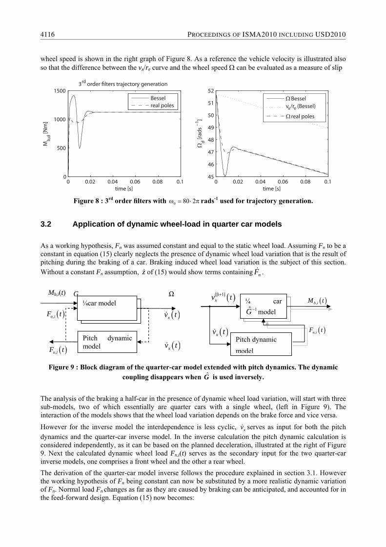
For Figure 8 the input for the trajectory shaping filters is a step in deceleration request from 0 to 09middotg The left axis shows the brake moment calculated with the Bessel filter as a solid line and the Mb from the real-poles filter as a dashed line Initially the brake is strongly engaged but after 10 ms a strong reduction follows This negative peak dynamically counteracts the tendency to wheel lock ( ) The desired 0Ω rarr
Vehicle
deceleration demand
Trajectory shaping filter
x d
v x dv
x dv
Inverse system
1flatGminus
1xv xv
dΩΩ
bMx dv
xvdriver
xv
switch
GCC
VEHICLE CONCEPT MODELLING 4115
wheel speed is shown in the right graph of Figure 8 As a reference the vehicle velocity is illustrated also so that the difference between the vxre curve and the wheel speed Ω can be evaluated as a measure of slip
0 002 004 006 008 010
500
1000
1500
time [s]
Mb
d [Nm
]
3rd order filters trajectory generation
0 002 004 006 008 0145
46
47
48
49
50
51
52
Ωd [r
ads
minus1 ]
time [s]
Besselreal poles
Bessel Ωv (Bessel)xre
real poles Ω
Figure 8 3rd order filters with 0 80 2ω = sdot π rads-1 used for trajectory generation
32 Application of dynamic wheel-load in quarter car models
As a working hypothesis Fn was assumed constant and equal to the static wheel load Assuming Fn to be a constant in equation (15) clearly neglects the presence of dynamic wheel load variation that is the result of pitching during the braking of a car Braking induced wheel load variation is the subject of this section Without a constant Fn assumption of z (15) would show terms containing nF
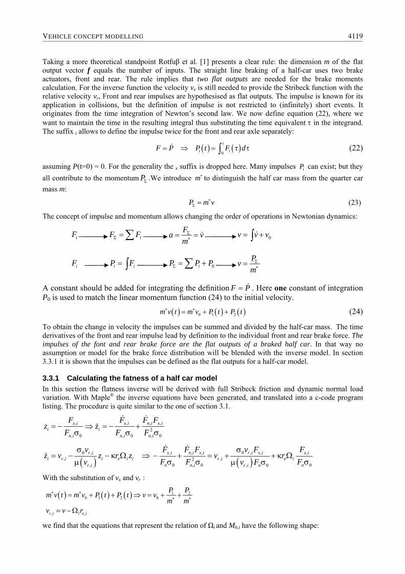
Figure 9 Block diagram of the quarter-car model extended with pitch dynamics The dynamic
coupling disappears when is used inversely G
The analysis of the braking a half-car in the presence of dynamic wheel load variation will start with three sub-models two of which essentially are quarter cars with a single wheel (left in Figure 9) The interaction of the models shows that the wheel load variation depends on the brake force and vice versa
However for the inverse model the interdependence is less cyclic xv serves as input for both the pitch dynamics and the quarter-car inverse model In the inverse calculation the pitch dynamic calculation is considered independently as it can be based on the planned deceleration illustrated at the right of Figure 9 Next the calculated dynamic wheel load Fni(t) serves as the secondary input for the two quarter-car inverse models one comprises a front wheel and the other a rear wheel The derivation of the quarter-car model inverse follows the procedure explained in section 31 However the working hypothesis of Fn being constant can now be substituted by a more realistic dynamic variation of Fn Normal load Fn changes as far as they are caused by braking can be anticipated and accounted for in the feed-forward design Equation (15) now becomes
frac14car model ( )n iF t
frac14car model
Pitch dynamic model
G
( )n iF t
Ω
( )xv t
Mbi(t)
( )xv t
frac14 car model
( )n iF t
frac14 car 1Gminus model
( )xv t
(( ) )1xv tβ+
( )b iM t
Pitch dynamic model
4116 PROCEEDINGS OF ISMA2010 INCLUDING USD2010
2
0 0 0
n i i xi x i xi i
n i i n i i n i i
F m vm v m vz zF F F
= rArr = +minus σ minus σ σ
Regenerating the c code by symbolic computation we find the inverse functions Ωi and Mbi Regenerating the c code by symbolic computation we find the inverse functions Ωi and Mbi
( ) i x x x n i n if v v v F FΩ = (20)
( ) b i e i i x i x x x x n i n i n iM r m v I f v v v v F F F= minus minus (21)
Leaving 3 extra inputs to be defined ( ) ( ) ( ) n i n i n iF t F t F t The front and rear axle load variations show
linear dependence on xv since the normal load ( )n iF t results from the linear differential equations with
xv as input Since the pitch dynamics has been described with linear differential equations we can obtain
using the same transfer function that resulted in ( )nF t ( )n iF t and use an order higher derivative of the
input use xv instead of xv as input
Table 2 Model parameters defining the vertical dynamics of the half car
0 02 04 06 08 13000
3500
4000
4500
5000
time[s]
Fn[N
]
Fn1 vx = minus5msminus2
Fn2 vx = minus5msminus2
Fn1 vx = minus9msminus2
Fn2 vx = minus9msminus2
parameter value Dimension
Iθ 1000 kgm2
cz 80000 Nm-1 kz 4000 Nsm-1 a 12 m b 15 m h 06 M
Figure 10 The dynamic wheel load during braking
By using quarter-car models for this calculation the contribution to the total deceleration of the vehicle depends on the static wheel load distribution The desired brake moment and wheel rotational velocity for the front and rear wheels are displayed in Figure 11 To guarantee that the requested deceleration is inside the domain D for the unloaded rear axle the deceleration was lowered to 65g It is a promising result that we can anticipate on a predicted wheel load change However in the top diagrams of Figure 11 the following phenomenon can be observed a reduction of vertical force instantaneously changes the brake force To maintain the constant brake force the tyre is demanded to compensate for the reduced vertical load by increasing the slip This can be seen in Figure 11(b) as the increased distance of Ω to vre at 01 seconds The increased slip value is reached by decelerating the wheel these low frequent variations can be seen in the brake torque Mb Figure 11a It can be shown that each wheel delivers an equal contribution of the brake force regardless of the changed normal load on the individual wheels This is a consequence of the fact that each wheel is related to a quarter-car model which is assumed to represent a given portion of the total mass of the vehicle The remaining question is whether this approach is desirable
VEHICLE CONCEPT MODELLING 4117
0 01 02 03 040
200
400
600
800
1000
1200
time [s]
Mb [N
m]
Wheel load dependent distribution
0 01 02 03 0440
45
50
55
time [s]
Ω [r
adsminus
1 ]
0 01 02 03 040
200
400
600
800
1000
1200
time [s]
Mb [N
m]
Fixed brake force distribution
M
bf
Mbr
0 01 02 03 0440
45
50
55
time [s]
Ω [r
adsminus
1 ]
Ω
f
Ωr
vxr
e
Figure 11 The desired brake torque and wheel rotational speed taking into account the dynamic wheel load reduction at the rear axle Desired deceleration lowered to 065 g τt 32ms polynomial
planning
In the bottom graphs of Figure 11 we assign a brake force proportional to the normal load on the specific wheel This can be emulated in the quarter car by introducing a time-varying quarter car mass
( ) ( )n ii
F tm t
g=
It is illustrated that the wheel slip behaviour complies with the criterion of being small and rather constant to ensure good road-holding Moreover it can be shown that with this proportionality zi loses its dependence on Fni and the derivation becomes similar to 31
33 The Flatness of a half car model
From the previous section it can be concluded that the quarter car model unintentionally fixes the brake force distribution with the definition of the quarter-car mass Introducing varying mass provides a provisional solution In this section we define two flat outputs Equation (4) shows that both brake forces contribute to the deceleration In an inverse approach the global deceleration will not discriminate the individual forces that have caused it The braked halve-car can never be inverted uniquely based on vx as a flat output In 32 information about the distribution between front and rear of the brake forces was added as a closing condition As these synthetic closing conditions are blended with the inverse model it loses it generality
4118 PROCEEDINGS OF ISMA2010 INCLUDING USD2010
Taking a more theoretical standpoint Rotfuβ et al [1] presents a clear rule the dimension m of the flat output vector f equals the number of inputs The straight line braking of a half-car uses two brake actuators front and rear The rule implies that two flat outputs are needed for the brake moments calculation For the inverse function the velocity vx is still needed to provide the Stribeck function with the relative velocity vr Front and rear impulses are hypothesised as flat outputs The impulse is known for its application in collisions but the definition of impulse is not restricted to (infinitely) short events It originates from the time integration of Newtonrsquos second law We now define equation (22) where we want to maintain the time in the resulting integral thus substituting the time equivalent τ in the integrand The suffix i allows to define the impulse twice for the front and rear axle separately
( ) ( )0
t
i iF P P t F= rArr = τint dτ (22)
assuming P(t=0) = 0 For the generality the x suffix is dropped here Many impulses can exist but they all contribute to the momentum We introduce
iPPΣ mlowast to distinguish the half car mass from the quarter car
mass m
P m vlowastΣ = (23)
The concept of impulse and momentum allows changing the order of operations in Newtonian dynamics
iF iF FΣ = sum Fa vm
Σlowast= = 0v v v= +int
iF 0iP PΣ
A constant should be added for integrating the definition F P= Here one constant of integration P0 is used to match the linear momentum function (24) to the initial velocity
( ) ( ) ( )0 1 2m v t m v P t P tlowast lowast= + + (24)
To obtain the change in velocity the impulses can be summed and divided by the half-car mass The time derivatives of the front and rear impulse lead by definition to the individual front and rear brake force The impulses of the font and rear brake force are the flat outputs of a braked half car In that way no assumption or model for the brake force distribution will be blended with the inverse model In section 331 it is shown that the impulses can be defined as the flat outputs for a half-car model
331 Calculating the fatness of a half car model In this section the flatness inverse will be derived with full Stribeck friction and dynamic normal load variation With Maplereg the inverse equations have been generated and translated into a c-code program listing The procedure is quite similar to the one of section 31
2
0 0 0
x i x ii i
n i n i n i
F Fz z
F F= minus rArr = minus +
σ σn i x iF F
F σ
( ) ( )0 0
20 0 0
r i x i n i x i r i x i x ii r i i e i i r i e i
n n i nr i r i n
v F F F v Fz v z r z v r
F F Fv vσ σ
= minus minus κ Ω rArr minus + = + + κ Ωσ σμ μ 0
FF σσ
With the substitution of vx and vr
( ) ( ) ( ) 1 2
0 1 2 0
r i i e i
P Pm v t m v P t P t v vm m
v v r
lowast lowastlowast lowast= + + rArr = + +
= minus Ω
we find that the equations that represent the relation of Ωi and Mbi have the following shape
P= +sum Pvmi iP F= int = Σ
lowast
VEHICLE CONCEPT MODELLING 4119
( ) i i i n i n iP P F FΩ = PF
( ) b i e i i i i n i n i n iM r P P P F F F= + P PF (25)
where In [ 1 2TP P=P ] (25) Fni is not a separate flat output The complete half-car model inverse
is composed similarly to the calculation scheme in Figure 9 The switch from the vector of flat outputs P to the scalar brake impulse Pi corresponding to the ith axle shows that the coupling is present in the low order time derivatives
Figure 12 Calculation scheme for half-car inverse
0 01 02 03 04 050
200
400
600
800
1000
1200
time [s]
Mb
d [Nm
]
Flatness based halfminuscar inverse
M
bf
Mbr
0 01 02 03 04 0535
40
45
50
55
time [s]
Ωd [r
adsminus
1 ]
Ω
f
Ωr
vxr
e
Figure 13 Half car inverse Independent front and rear force planning example Fbf=3396 N
Fbr=1953 N with both 23 ms transition time in polynomial planning 068g deceleration planned equivalent to Figure 11
In Figure 13 the half car inverse model calculates Mb and wheel speed Ω for front and rear wheels respectively Left right symmetry during the manoeuvre has been assumed thus equal values are calculated for both wheels on one axle The brake force contribution of each axle can now be planned independently In this simple example a brake force set point Fb1=3396 N has been chosen for the front axle Fb2=1953 N with both 23 ms transition time in polynomial planning P1 and P2 are found as the time integrals of the independently planned brake forces The two target brake forces togetter result in a 068g deceleration so that their mutual effect is equivalent to Figure 11
1 1 1 n n nF F F⎡ ⎤⎣ ⎦
1ˆfGminus model
frac12 car Pitch model
( ) ( )t t⎡ ⎤⎣ ⎦P P
( ) ( ) ( ) ( ) t t t t⎡ ⎤⎣ ⎦P P P P ( )1bM t
1ˆrGminus model ( )2bM t
2 2 2 n n nF F F⎡ ⎤⎣ ⎦
( ) ( ) ( ) ( )1 1 t t P t P t⎡ ⎤⎣ ⎦P P
( ) ( ) ( ) ( )2 2 t t P t P t⎡ ⎤⎣ ⎦P P
4120 PROCEEDINGS OF ISMA2010 INCLUDING USD2010
4 First Implementation results
In the Laboratory of Delft University a drum test rig allows indoor testing of a single braked wheel The system is driven by a large steel drum located under the tyre The axle height is constrained so that the vertical load can be adjusted only statically The wheel axle is braked by a conventional brake disc and a caliper whose hydraulic pressure can be servo-controlled This system comprises analog electronics and receives the desired brake pressure from a high hierarchy D-Space control system The wheel-axle being supported by load sensing platforms just above two axle bearings the brake torque can be measured in a connecting axle between brake disc and the wheel Also the wheel speed can be measured accurately using an industrial optical encoder
wheel velocityencoder
25 m drum
Piezo electricelements
frame
disc brake
flexibleconnections
torque sensor
tyre
Figure 14 Drawing of front view of the single braked wheel on the drum test-rig
Ideally the inertia of the test drum with a 25 m diameter represents the quarter car mass Unfortunately the inertia is a factor 16 larger The controller of the electromotor of the drum can be asked to track a rapidly decreasing vehicle velocity reference It will then mimic the deceleration of the quarter car by electrical braking of the drum while performing a brake experiment
Brake Torque Sensor Brake caliper
Figure 15 Photos of the drum test rig with a single braked wheel in TU Delft Laboratory
The parameters of the tyre have been estimated in dedicated experiments before The inverse model has been used to calculate a brake torque signal that delivers brake force according to a desired trajectory A shaping filter has been implemented to provide the required smoothness of the flat output ie the input of the inverse
Brake pressure signal Brake Disk
Pad
Disk
Infrared thermometer Encoder
VEHICLE CONCEPT MODELLING 4121
09 1 110
5
10
15
20
Time [s]
Pre
ssur
e [b
ar]
Brake pressure response (n = 9)
Desired pressureActual pressure
09 1 110
5
10
15
20
Time [s]
Pre
ssur
e [b
ar]
Brake pressure response (n = 11)
Desired pressureActual pressure
Figure 16 The brake caliper pressure control left step response rigtht the desired brake torque
calmed down by putting the poles of the shaping filter at -322π rads-1
From the initial tests we observe the limitations in the time response of the brake system a time lag occurs and the pressure rate is limited as can be seen from the left graph of Figure 16 Taking into account these actuator limitations the poles of the shaping filter have been decreased to -322π rads-1 in order to slow down the desired brake pressure response allowing a better tracking by the actual brake pressure in the right graph of Figure 16
0 05 1 15 2 25200
400
600
800
1000Avarage brake force minusFx (n = 12)
Time [s]
minusFx
[N]
Figure 17 The brake force averaged over 12 repeated experiments
The brake force signal in Figure 17 is quite disturbed by harmonic force components that could be a result of unbalance or varying properties around the tyre circumference The transition of the brake force is so dynamic that low-pass filtering would influence the measured signal Therefore averaging has been applied Both random measurement errors and harmonic components should be reduced by averaging many responses provided that the harmonic features are randomly spaced in phase Still the force response of the system is disappointing The brake torque control is held responsible since already the calliper pressure doesnt follow the intended time response
4122 PROCEEDINGS OF ISMA2010 INCLUDING USD2010
Conclusions
The quarter car model with LuGre tire can be inverted to obtain a feed-forward control signal The inversion fits the framework of flatness where a fictitious output can be selected for the quarter car it has been proven that vx is the flat output This output needs to be planned andor controlled Based on the flat output and a number of time derivatives the input is the result of an algebraic inverse function Special attention is needed to the domain of validity of the original to flat state transformation and the domain of the inverse relation (not discussed in detail here) The assumption of a constant normal load that is an element in the quarter car flatness is not very realistic Therefore a half car with dynamic load transfer has been developed The application of the dynamic normal load variation in a tandem of quarter cars without reconsidering the brake force distribution lead to unsatisfactory results To avoid the brake force distribution even as an implicit assumption to be blended with the inverse calculation an inverse with two outputs needs two inputs It has been shown that the impulse of both front brake force and rear brake force can serve as flat outputs of the half car model and an inverse model can be established using these flat outputs as the inputs of the inverse Creating feedback control on the flat states besides the feed-forward presented here may become feasible when force-sensing bearings (FSB) become available
Recommendations
The initial results on the drum test rig show that the brake actuation limitations stand in the way of validating the presented feed-forward control To improve the brake control we propose to reduce the length of the brake hose and replace it with a metal braided brake hose Further one should remove the analogue electronics and control the servo valve in the brake system directly from the high hierarchy D-space
References
[1] Ralf Rotfuszlig Joachim Rudolph Michael Zeitz Flachheit Ein neuer Zugang zur Steuerung und Reglung nichtlinearer Systeme in Automatisierungstechnik 45 vol 11 1997 pp 517-525
[2] Erik Vermeer Model based Wheel Speed Controller Design MSc thesis TU Delft 2005 [3] Brian Armstrong-Heacutelouvry Pierre Dupont Carlos Canudas de Witt A Survey of Models
Analysis Tools and Compensation Methods for the Control of Machines with Friction Automatica Vol 30 no 7 pp 1083-1138 1994
[4] DP Hess A Soom Friction at a Lubrificated line contact operating at oscillating Sliding Velocities Journal of Tribology Vol 112 pp 147-152 January 1990
[5] Canudas de Wit C Tsiotras P Velenis E Basset M and Gissinger G lsquoDynamic friction models for road tyre longitudinal interactionrsquo Vehicle System Dynamics vol 39 no 3 pp 189-226 2003
[6] De Vries EJH Fehn A Rixen DJ lsquoFlatness-based model inverse for feed-forward braking controlrsquo lsquosupplement to Vehicle System Dynamicsrsquo vol 4X no X 2010 (in press)
[7] De Vries EJH Rixen DJ lsquoFlatness-based model inverse for feed-forward braking controlrsquo proceedings XXI iavsd2009 congress Stockholm 17-21 august 2009
[8] Sunil K Agarwal Hebertt J Sira Ramiacuterez Differentially Flat Systems Marcel Dekker Inc New York 2004
[9] Jean Levine Analysis and Control of Nonlinear Systems a Flatness-based Approach Springer Berlin Heidelberg 2009
VEHICLE CONCEPT MODELLING 4123
()(
)2
220
2
22
00
00
220
4()
(()
()
22
()
()2
()
()
()
()()2
()()
()
4()
bx
cx
x
nc
xcx
xs
sx
sx
cx
xx
xcx
cx
bb
acM
mrv
tJ
mr
vt
mr
vt
aFr
vt
mr
vt
mrvt
mrv
vt
mrv
vt
mr
vtvt
mrvtvt
mrvt
mr
vt
mr
v
minus+
minus=
minusminus
κμminus
σ+
minusμσ
+κμ
minusσ
+κμ
minusσ
+κμ
minusσ
minusμ
+
minusκμ
minusσ
+
hellip
()(
)(
)
22
00
00
00
00
()
()
()
()()
()()
()
()()
22
()
()
()
()()2
()()
()
2
xnss
xnc
xs
xx
xx
ssx
cx
x
nss
nc
xs
sx
sx
cx
xx
xcx
nc
tFv
vt
Fvt
mv
vtvt
mvtvt
mv
vt
mvtvt
Frv
Fr
vt
mrv
vt
mrv
vt
mr
vtvt
mrvtvt
mrvt
Fr
minusμσ
minusμσ
minusσ
minusσ
minusμ
minusμ
+
μσ
+μσ
minusκμ
+σ
minusκμ
+σ
+μ
times
μ
hellip
hellip
()
()
22
00
00
22
20
0
20
00
()
()2
()
()
()
()()2
()()
()
4()
()
()2
()()
()2
xcx
xs
sx
sx
cx
xx
xcx
nc
cx
x
nss
xnc
xx
sx
vt
mr
vt
mrvt
mrv
vt
mrv
vt
mr
vtvt
mrvtvt
mrvt
Fr
mr
vt
mr
vt
Fv
vt
Fvtvt
mv
vt
σminus
κμ+
σminus
κμ+
σminus
κμ+
σ+
μminus
minusμσ
+κμ
minusσ
times
minusμσ
minusμσ
minusσ
minus
hellip
hellip
(
)
()
22
00
0
2
22
20
0
()()
()()
()()
()
()()
()()
42
2
()
()
xx
sx
xx
xssx
cx
xcx
x
nc
cx
x
mvtvt
mv
vtvt
mvtvt
mv
vt
mvtvt
mvtvt
bac
a
aFr
mr
vt
mr
vt
bF⎛
⎞⎜
⎟⎛
⎞⎜
⎟⎜
⎟⎜
⎟⎜
⎟⎜
⎟⎜
⎟⎜
⎟⎜
⎟⎜
⎟⎜
⎟⎜
⎟⎜
⎟⎜
⎟⎜
⎟⎜
⎟⎜
⎟⎜
⎟⎜
⎟⎜
⎟σ
minusσ
minusσ
minusμ
minusμ
minusμ
⎝⎠
⎜⎟
⎜⎟
minus⎜
⎟⎝
⎠
=minus
μσ
+κμ
minusσ
=
()
()
00
00
22
00
00
2()
()
()
()()2
()()
()
()
()
()()
()()
()
()()
nss
nc
xs
sx
sx
cx
xx
xcx
nss
xnc
xs
xx
xx
ssx
cx
x
rvFr
vt
mrv
vt
mrv
vt
mr
vtvt
mrvtvt
mrvt
cFv
vt
Fvt
mv
vtvt
mvtvt
mv
vt
mvtvt
μσ
+μσ
minusκμ
+σ
minusκμ
+σ
+μ
=minus
μσ
minusμσ
minusσ
minusσ
minusμ
minusμ
Apendix (A1)
4124 PROCEEDINGS OF ISMA2010 INCLUDING USD2010
2 Development of a simple half car model
The straight line motion allows us to consider just one half of a left-right symmetrical car Such model takes into account the pitching and the additional loading of the front axle during braking Conversely the rear axle-load is reduced during braking In the horizontal direction front and rear tyre models provide the brake force in response to the wheel slip The LuGre tyre model describes the brake force generation on both wheels The weight of the unsprung masses is neglected the vertical tyre-load variation will contain low frequencies due to the absence of the wheel-hop mode in the model Furthermore the road is assumed to be flat Without loosing generality for abbreviation in the paper the front and rear axle properties and the front and rear tyre parameters have been considered identical on both axles
Figure 1 The half-car model
First the vertical and pitch dynamics have been derived
( ) ( )( )( ) ( ) ( ) ( ) (
( ) ( ) ( ) ( )
2 2 2 21 2
1 2
2 2
and
z z z z
x x z z z z
n z z n z z
my mg k y c y k a b c a b
I h y F F k a b y c a b y k a b c a b
F k y a c y a F k y b c y b
= minus minus minus minus θ minus minus θ
θ = minus minus + minus minus minus minus minus + θ minus + θ
= + θ + + θ = minus θ + minus θ
)
(1)
(2)
(3)
Here y denotes the vertical degree of freedom of the centre of gravity x denotes the horizontal direction and vx is the vehicle speed taken positive in driving direction The pitch degree of freedom is denoted with θ The suspension stiffness is denoted cz and the damping kz The front and rear axle are located at a distance of a and b with respect to the centre of gravity Fn denotes the normal load and Fx is the longitudinal force taken positive in driving direction Braking typically results in a negative Fx An additional suffix i is introduced showing a 1 for the front axle and a 2 for the rear axle The moment arm (hminusy) of the brake forces will be approximated with h so by neglecting products of variations non-linearity in the pitch model has been avoided The brake forces are calculated with the LuGre tyre model that introduces an internal deformation state zi as the basis for the force calculation
( )
1 2 0
0
0
with x x x x i n i
i i e n i i b i
r i ii r i e i i
r i
mv F F F F z
I r F z M
v zz v r z
v
= + = minus σ
Ω = σ minus
σ= minus minus κ Ω
μ
i
(4)
(5)
(6)
The wheel speed is given by Ω the relative speed at the contact point is defined by
4110 PROCEEDINGS OF ISMA2010 INCLUDING USD2010
r i x i ev v r= minus Ω (7)
σ0 is a normalized tyre stiffness parameter The LuGre damping parameters σ1 and σ2 have been assumed zero Still good correspondence could be found between the LuGre model and measured stationary tyre characteristic κ introduces lsquoconvection lossrsquo to the tyre deformation The complexity of the Stribeck friction description ( )rvμ has a strong influence on the feasibility of the inverse dynamic system therefore Vermeer [2] after [3][4] proposes a simple friction law (8) as an alternative for the more common normal function or exponential decaying functions
( ) c r s sr
r s
vv
v vvμ + μ
μ =+
(8)
A strictly positive value can be assigned to the parameter vs and the | | sign on vr can be dropped since vr gt 0 is ensured during braking
21 Reduction to a quarter car
Assuming a constant normal load and using in equation (4) a quarter car mass that is being decelerated by the brake force Fxi the above equations for the LuGre tyre can constitute a quarter car model with a single braked wheel The quarter-car mass represents the static wheel load of front or rear wheel and thus depends on the centre of gravity location The mass thus differs from the exact quarter vehicle mass
14
0x nm v F z= minusσ (9)
Figure 2 Transition from initial steady state to desired steady state xvminus and have been
drawn to comply with their physical direction during braking bF = minus xF
3 Definition of flatness
Some definitions of flatness take vector-algebra as the language to establish the definition We have an engineering viewpoint The next definition follows Rotfuβ et al [1] Definition 1 Flatness of nonlinear systems A nonlinear system
( ) ( ) 0 0 ( ) ( )n mt t= = isinx F x u x x x u isin (10)
is called flat if there exists a (possibly fictitious) output
VEHICLE CONCEPT MODELLING 4111
( 1 Tm )f f=f hellip (11)
with ( ) ( )dim dimm= =f u that fulfills the following conditions
bull The fictitious output f is defined by a nonlinear function ϕ of the states x the inputs ui and a
finite number of their time derivatives ( )kiu k = 1hellipαi
( )( )1 =f x u u αϕ hellip (12)
bull The states x and the input u can be described by the nonlinear functions φ and ψ of the fictitious output f (see equation (11)) and a finite number of its time derivatives
( )( ) =x f f f βφ hellip (13)
( )( )1 +=u f f f βψ hellip (14)
If these conditions are satisfied at least locally1 then the (possibly fictitious) output is called flat output and the system is flat For abbreviation the so-called multi-index ( )β has been used to denote the order of differentiation for each flat output fi in the above equation Equation (14) is called the inverse system since it describes the input u as function of the flat output ( )tf and a number of its time derivatives Sometimes this flatness is referred to as ldquothe inverse does not have any dynamicsrdquo [8] which means that the calculation of the input u from (14) is purely algebraic It has been proven by Rotfuβ in [1] that the condition of linear independent flat outputs can always be guaranteed when ( ) ( )dim dimm= =f u
31 Flatness of the LuGre model with vx as flat output
The quarter car model with a single braked wheel uses one input the brake torque Mb It is clear from that the flat output will be a scalar variable that can generically be denoted f ( ) ( )dim dim 1=u f =
In this section it is hypothesised the vx is the flat output f for the quarter-car model with LuGre tyre model To proof this hypothesis all system states (vxzΩ) and the input Mb must be calculated based on vx and a finite number of its time derivatives ie find φ and ψ of (13) and (14) First a block diagram of the brake actuation of a quarter-car model with a generic non-linear tyre is given in Figure 3
Eulerrsquos Law Slip definition
Figure 3 Schematic illustration of the calculations in the quarter-car model with an unspecified
stationary tyre model
1 The bounded domain and range of φ and domain of ψ can restrict the validity to a subset of n
Ω Ω M IΣ = Ω
λ x e
x
v rvminus Ω
λ =
re
ndash
dtΩint
Tyre characteristic Newtonrsquos Law Mb
x xF mv=
|Fx|
λ xv dtint
v x
4112 PROCEEDINGS OF ISMA2010 INCLUDING USD2010
The general principle of the inverse calculation is illustrated with the flow chart of Figure 4
Newtonrsquos Law Tyre characteristic Slip definition
Ω
Figure 4 Schematic illustration of the inverse model calculations for a model containing an
unspecified stationary tyre model
The actual calculation will be performed with the LuGre tyre model that contains a deformation state z Therefore this LuGre model shows a transient tyre force response that differs from its stationary non-linear tyre characteristic
Figure 5 Calculation scheme for the LuGre tyre model
Flatness of the quarter-car with the LuGre tyre model can be proven using the following steps Equation (4) is rewritten and derived with respect to time under the working hypothesis of Fn being constant for the quarter car model
0 0
x
n n
mv mvz zF F
= rArr = x
minus σ minus σ (15)
This variable z and its time derivative can be substituted in the original description of the LuGre deformation state derivative (6)
( )0
0 0( )r x r x
r e r er n r n
v mv v mv mvz v z r z v rv F v F
σ= minus minus κ Ω rArr = + minus κΩ
μ minus σ μx
nFminus σ
The relative velocity is replaced by (7) and substituting ( )rvμ of equation (8) results in
( )( )( )( )0 0
s x e x e xx xx e e
n nc x e s s n
v v r v r mvmv mvv r rF Fv r v F
+ minus Ω minus Ω= minus Ω + minus κΩ
minus σ minus σμ minus Ω + μ (16)
( )( ) ( ) ( )( )( )( ) ( )( )
0
0
c x e s s x n x e c x e s s
s x e x e x e x c x e s s
v r v mv F v r v r v
v v r v r mv r mv v r v
μ minus Ω + μ = minus σ minus Ω μ minus Ω + μ minus
σ + minus Ω minus Ω minus κΩ μ minus Ω + μ
hellip (17)
xv λ Ωx xF mv= x e
e
v rr
minus Ωλ =
Ω d
dt I
re
ndash
|Fx| ddt
λ
xv Mb
Newtonrsquos Law Tyre model Mb
x xF mv= xv ddt
Ω
re
I Ω ndash
LuGre-1 zz⎫⎬⎭
Fx ddt
VEHICLE CONCEPT MODELLING 4113
The roots equation obtained from (17) give an algebraic equation for Ω depending on [ From the two roots the largest wheel speed is selected
] x x xv v v
minus12minus10
minus8minus6
minus4minus2
0
0
10
20
30
40
500
20
40
60
80
100
120
140
160
vx [msminus1]
Gminus1
isomorphism on bounded domain
vx[msminus2]
Ω[r
adsminus
1]
Figure 6 The essential part of state transformation 2φ where the steady-state of constant deceleration is used ( 0xv )= to draw Ω as a function of 0+ minus⎡ ⎤isin ⎣ ⎦z
( ) ( ) ( ) ( )( )( )
( ) ( )( ) ( )( )
2
2 2 20 0
0 0 0 0
20 0 0
4where
2
( ) ( )
2 ( ) ( ) ( ) ( ) ( ) 2 ( ) ( ) ( )
( ) ( ) (
n c c x x
n s s n c x s s x s x c x x x x c x
n s s x n c x s x
b b a c
a
a F r mr v t mr v t
b F rv F r v t mrv v t mrv v t mr v t v t mr v t v t mr v t
c F v v t F v t mv v t
minus + minusΩ =
= minus μ σ + κμ minus σ
= μ σ + μ σ minus κμ + σ minus κμ + σ + μ
= minus μ σ minus μ σ minus σ
z z z z
z
z
z
z ( )20) ( ) ( ) ( ) ( ) ( ) ( )x x x s s x c x xv t m v t v t mv v t m v t v tminus σ minus μ minus μ
(18)
And thus the transformation from flat states to the original states is complete
( )1
+ root of eqn(18)eqn(15)
z⎡ ⎤⎢ ⎥⎢ ⎥⎢ ⎥⎣ ⎦
x = zφ = (19)
From (19) it can be seen that and are simple trivial expressions The function for Ω 1φ 3φ 2φ (18) is more
complicated In Figure 6 the transformation based on varying flat states xv and xv is illustrated Ω is plotted on the vertical axis in relation to both deceleration and velocity on the x- and y-axis respectively Although the isomorphism is to be developed on a three dimensional state space to + minus⎡ ⎤isin sub ⎣ ⎦z D
4114 PROCEEDINGS OF ISMA2010 INCLUDING USD2010
enable the visualisation of Ω has been used first in 3 0xv z= = Figure 6 The condition 3 0xv z= = defines the steady-state of constant deceleration The curve in the x-y plane of the graph in Figure 6 defines the bound of allowable decelerations at a given velocity One can now find the inverse system ψ for Mb it results in expression equation (A1)
( ) ( ) appendix eqn(A1)b x x x xw M v v v v= =zψ
This result yields the proof of flatness of the quarter-car with the LuGre tyre model for the flat output vx The validity of the proof is restricted to the sub-space D where ψ and φ are defined The software code to make the calculation is generated with help of symbolic computation in Maplereg
311 Simulation results From the concept of flatness and the inverse equations that have been derived we observe that the raw input needs to be smoothened so that higher order derivatives exist and are finite In this case the term xv contributes in the brake torque and thus it is required to ensure xv to be continuous if a continuous brake torque is desired Since the inverse calculations are algebraic equations on the flat states and the derivatives the state derivatives need to be provided to the inverse model The future desired behaviour of the vehicle system can now be planned and characterised by ( )x dv t In the literature [8] polynomial planning over fixed transition intervals is very common In [6][7] we propose the use of shaping filters to reach the desired smoothness on and to blend the time-derivations with the filter In ( )x dv t Figure 7 this procedure is illustrated Since the aim is to control vehicle deceleration the velocity vx is taken from the vehicle instead of from the planning The deceleration will affect the real vehicle speed
Figure 7 control strategy with quarter-car variables
The system is parameterized using the values given in Table 1 Table 1 Quarter-car model parameters
parameter value Ref parameter value ref
M 400 kg κ 367 m-1 [5]
Fn 4000 N μs 12 σ0 18154 m-1 [2]
μc 07 σ1 0 vstribeck 657 [2]σ2 0 vx0 16 ms-1
For Figure 8 the input for the trajectory shaping filters is a step in deceleration request from 0 to 09middotg The left axis shows the brake moment calculated with the Bessel filter as a solid line and the Mb from the real-poles filter as a dashed line Initially the brake is strongly engaged but after 10 ms a strong reduction follows This negative peak dynamically counteracts the tendency to wheel lock ( ) The desired 0Ω rarr
Vehicle
deceleration demand
Trajectory shaping filter
x d
v x dv
x dv
Inverse system
1flatGminus
1xv xv
dΩΩ
bMx dv
xvdriver
xv
switch
GCC
VEHICLE CONCEPT MODELLING 4115
wheel speed is shown in the right graph of Figure 8 As a reference the vehicle velocity is illustrated also so that the difference between the vxre curve and the wheel speed Ω can be evaluated as a measure of slip
0 002 004 006 008 010
500
1000
1500
time [s]
Mb
d [Nm
]
3rd order filters trajectory generation
0 002 004 006 008 0145
46
47
48
49
50
51
52
Ωd [r
ads
minus1 ]
time [s]
Besselreal poles
Bessel Ωv (Bessel)xre
real poles Ω
Figure 8 3rd order filters with 0 80 2ω = sdot π rads-1 used for trajectory generation
32 Application of dynamic wheel-load in quarter car models
As a working hypothesis Fn was assumed constant and equal to the static wheel load Assuming Fn to be a constant in equation (15) clearly neglects the presence of dynamic wheel load variation that is the result of pitching during the braking of a car Braking induced wheel load variation is the subject of this section Without a constant Fn assumption of z (15) would show terms containing nF
Figure 9 Block diagram of the quarter-car model extended with pitch dynamics The dynamic
coupling disappears when is used inversely G
The analysis of the braking a half-car in the presence of dynamic wheel load variation will start with three sub-models two of which essentially are quarter cars with a single wheel (left in Figure 9) The interaction of the models shows that the wheel load variation depends on the brake force and vice versa
However for the inverse model the interdependence is less cyclic xv serves as input for both the pitch dynamics and the quarter-car inverse model In the inverse calculation the pitch dynamic calculation is considered independently as it can be based on the planned deceleration illustrated at the right of Figure 9 Next the calculated dynamic wheel load Fni(t) serves as the secondary input for the two quarter-car inverse models one comprises a front wheel and the other a rear wheel The derivation of the quarter-car model inverse follows the procedure explained in section 31 However the working hypothesis of Fn being constant can now be substituted by a more realistic dynamic variation of Fn Normal load Fn changes as far as they are caused by braking can be anticipated and accounted for in the feed-forward design Equation (15) now becomes
frac14car model ( )n iF t
frac14car model
Pitch dynamic model
G
( )n iF t
Ω
( )xv t
Mbi(t)
( )xv t
frac14 car model
( )n iF t
frac14 car 1Gminus model
( )xv t
(( ) )1xv tβ+
( )b iM t
Pitch dynamic model
4116 PROCEEDINGS OF ISMA2010 INCLUDING USD2010
2
0 0 0
n i i xi x i xi i
n i i n i i n i i
F m vm v m vz zF F F
= rArr = +minus σ minus σ σ
Regenerating the c code by symbolic computation we find the inverse functions Ωi and Mbi Regenerating the c code by symbolic computation we find the inverse functions Ωi and Mbi
( ) i x x x n i n if v v v F FΩ = (20)
( ) b i e i i x i x x x x n i n i n iM r m v I f v v v v F F F= minus minus (21)
Leaving 3 extra inputs to be defined ( ) ( ) ( ) n i n i n iF t F t F t The front and rear axle load variations show
linear dependence on xv since the normal load ( )n iF t results from the linear differential equations with
xv as input Since the pitch dynamics has been described with linear differential equations we can obtain
using the same transfer function that resulted in ( )nF t ( )n iF t and use an order higher derivative of the
input use xv instead of xv as input
Table 2 Model parameters defining the vertical dynamics of the half car
0 02 04 06 08 13000
3500
4000
4500
5000
time[s]
Fn[N
]
Fn1 vx = minus5msminus2
Fn2 vx = minus5msminus2
Fn1 vx = minus9msminus2
Fn2 vx = minus9msminus2
parameter value Dimension
Iθ 1000 kgm2
cz 80000 Nm-1 kz 4000 Nsm-1 a 12 m b 15 m h 06 M
Figure 10 The dynamic wheel load during braking
By using quarter-car models for this calculation the contribution to the total deceleration of the vehicle depends on the static wheel load distribution The desired brake moment and wheel rotational velocity for the front and rear wheels are displayed in Figure 11 To guarantee that the requested deceleration is inside the domain D for the unloaded rear axle the deceleration was lowered to 65g It is a promising result that we can anticipate on a predicted wheel load change However in the top diagrams of Figure 11 the following phenomenon can be observed a reduction of vertical force instantaneously changes the brake force To maintain the constant brake force the tyre is demanded to compensate for the reduced vertical load by increasing the slip This can be seen in Figure 11(b) as the increased distance of Ω to vre at 01 seconds The increased slip value is reached by decelerating the wheel these low frequent variations can be seen in the brake torque Mb Figure 11a It can be shown that each wheel delivers an equal contribution of the brake force regardless of the changed normal load on the individual wheels This is a consequence of the fact that each wheel is related to a quarter-car model which is assumed to represent a given portion of the total mass of the vehicle The remaining question is whether this approach is desirable
VEHICLE CONCEPT MODELLING 4117
0 01 02 03 040
200
400
600
800
1000
1200
time [s]
Mb [N
m]
Wheel load dependent distribution
0 01 02 03 0440
45
50
55
time [s]
Ω [r
adsminus
1 ]
0 01 02 03 040
200
400
600
800
1000
1200
time [s]
Mb [N
m]
Fixed brake force distribution
M
bf
Mbr
0 01 02 03 0440
45
50
55
time [s]
Ω [r
adsminus
1 ]
Ω
f
Ωr
vxr
e
Figure 11 The desired brake torque and wheel rotational speed taking into account the dynamic wheel load reduction at the rear axle Desired deceleration lowered to 065 g τt 32ms polynomial
planning
In the bottom graphs of Figure 11 we assign a brake force proportional to the normal load on the specific wheel This can be emulated in the quarter car by introducing a time-varying quarter car mass
( ) ( )n ii
F tm t
g=
It is illustrated that the wheel slip behaviour complies with the criterion of being small and rather constant to ensure good road-holding Moreover it can be shown that with this proportionality zi loses its dependence on Fni and the derivation becomes similar to 31
33 The Flatness of a half car model
From the previous section it can be concluded that the quarter car model unintentionally fixes the brake force distribution with the definition of the quarter-car mass Introducing varying mass provides a provisional solution In this section we define two flat outputs Equation (4) shows that both brake forces contribute to the deceleration In an inverse approach the global deceleration will not discriminate the individual forces that have caused it The braked halve-car can never be inverted uniquely based on vx as a flat output In 32 information about the distribution between front and rear of the brake forces was added as a closing condition As these synthetic closing conditions are blended with the inverse model it loses it generality
4118 PROCEEDINGS OF ISMA2010 INCLUDING USD2010
Taking a more theoretical standpoint Rotfuβ et al [1] presents a clear rule the dimension m of the flat output vector f equals the number of inputs The straight line braking of a half-car uses two brake actuators front and rear The rule implies that two flat outputs are needed for the brake moments calculation For the inverse function the velocity vx is still needed to provide the Stribeck function with the relative velocity vr Front and rear impulses are hypothesised as flat outputs The impulse is known for its application in collisions but the definition of impulse is not restricted to (infinitely) short events It originates from the time integration of Newtonrsquos second law We now define equation (22) where we want to maintain the time in the resulting integral thus substituting the time equivalent τ in the integrand The suffix i allows to define the impulse twice for the front and rear axle separately
( ) ( )0
t
i iF P P t F= rArr = τint dτ (22)
assuming P(t=0) = 0 For the generality the x suffix is dropped here Many impulses can exist but they all contribute to the momentum We introduce
iPPΣ mlowast to distinguish the half car mass from the quarter car
mass m
P m vlowastΣ = (23)
The concept of impulse and momentum allows changing the order of operations in Newtonian dynamics
iF iF FΣ = sum Fa vm
Σlowast= = 0v v v= +int
iF 0iP PΣ
A constant should be added for integrating the definition F P= Here one constant of integration P0 is used to match the linear momentum function (24) to the initial velocity
( ) ( ) ( )0 1 2m v t m v P t P tlowast lowast= + + (24)
To obtain the change in velocity the impulses can be summed and divided by the half-car mass The time derivatives of the front and rear impulse lead by definition to the individual front and rear brake force The impulses of the font and rear brake force are the flat outputs of a braked half car In that way no assumption or model for the brake force distribution will be blended with the inverse model In section 331 it is shown that the impulses can be defined as the flat outputs for a half-car model
331 Calculating the fatness of a half car model In this section the flatness inverse will be derived with full Stribeck friction and dynamic normal load variation With Maplereg the inverse equations have been generated and translated into a c-code program listing The procedure is quite similar to the one of section 31
2
0 0 0
x i x ii i
n i n i n i
F Fz z
F F= minus rArr = minus +
σ σn i x iF F
F σ
( ) ( )0 0
20 0 0
r i x i n i x i r i x i x ii r i i e i i r i e i
n n i nr i r i n
v F F F v Fz v z r z v r
F F Fv vσ σ
= minus minus κ Ω rArr minus + = + + κ Ωσ σμ μ 0
FF σσ
With the substitution of vx and vr
( ) ( ) ( ) 1 2
0 1 2 0
r i i e i
P Pm v t m v P t P t v vm m
v v r
lowast lowastlowast lowast= + + rArr = + +
= minus Ω
we find that the equations that represent the relation of Ωi and Mbi have the following shape
P= +sum Pvmi iP F= int = Σ
lowast
VEHICLE CONCEPT MODELLING 4119
( ) i i i n i n iP P F FΩ = PF
( ) b i e i i i i n i n i n iM r P P P F F F= + P PF (25)
where In [ 1 2TP P=P ] (25) Fni is not a separate flat output The complete half-car model inverse
is composed similarly to the calculation scheme in Figure 9 The switch from the vector of flat outputs P to the scalar brake impulse Pi corresponding to the ith axle shows that the coupling is present in the low order time derivatives
Figure 12 Calculation scheme for half-car inverse
0 01 02 03 04 050
200
400
600
800
1000
1200
time [s]
Mb
d [Nm
]
Flatness based halfminuscar inverse
M
bf
Mbr
0 01 02 03 04 0535
40
45
50
55
time [s]
Ωd [r
adsminus
1 ]
Ω
f
Ωr
vxr
e
Figure 13 Half car inverse Independent front and rear force planning example Fbf=3396 N
Fbr=1953 N with both 23 ms transition time in polynomial planning 068g deceleration planned equivalent to Figure 11
In Figure 13 the half car inverse model calculates Mb and wheel speed Ω for front and rear wheels respectively Left right symmetry during the manoeuvre has been assumed thus equal values are calculated for both wheels on one axle The brake force contribution of each axle can now be planned independently In this simple example a brake force set point Fb1=3396 N has been chosen for the front axle Fb2=1953 N with both 23 ms transition time in polynomial planning P1 and P2 are found as the time integrals of the independently planned brake forces The two target brake forces togetter result in a 068g deceleration so that their mutual effect is equivalent to Figure 11
1 1 1 n n nF F F⎡ ⎤⎣ ⎦
1ˆfGminus model
frac12 car Pitch model
( ) ( )t t⎡ ⎤⎣ ⎦P P
( ) ( ) ( ) ( ) t t t t⎡ ⎤⎣ ⎦P P P P ( )1bM t
1ˆrGminus model ( )2bM t
2 2 2 n n nF F F⎡ ⎤⎣ ⎦
( ) ( ) ( ) ( )1 1 t t P t P t⎡ ⎤⎣ ⎦P P
( ) ( ) ( ) ( )2 2 t t P t P t⎡ ⎤⎣ ⎦P P
4120 PROCEEDINGS OF ISMA2010 INCLUDING USD2010
4 First Implementation results
In the Laboratory of Delft University a drum test rig allows indoor testing of a single braked wheel The system is driven by a large steel drum located under the tyre The axle height is constrained so that the vertical load can be adjusted only statically The wheel axle is braked by a conventional brake disc and a caliper whose hydraulic pressure can be servo-controlled This system comprises analog electronics and receives the desired brake pressure from a high hierarchy D-Space control system The wheel-axle being supported by load sensing platforms just above two axle bearings the brake torque can be measured in a connecting axle between brake disc and the wheel Also the wheel speed can be measured accurately using an industrial optical encoder
wheel velocityencoder
25 m drum
Piezo electricelements
frame
disc brake
flexibleconnections
torque sensor
tyre
Figure 14 Drawing of front view of the single braked wheel on the drum test-rig
Ideally the inertia of the test drum with a 25 m diameter represents the quarter car mass Unfortunately the inertia is a factor 16 larger The controller of the electromotor of the drum can be asked to track a rapidly decreasing vehicle velocity reference It will then mimic the deceleration of the quarter car by electrical braking of the drum while performing a brake experiment
Brake Torque Sensor Brake caliper
Figure 15 Photos of the drum test rig with a single braked wheel in TU Delft Laboratory
The parameters of the tyre have been estimated in dedicated experiments before The inverse model has been used to calculate a brake torque signal that delivers brake force according to a desired trajectory A shaping filter has been implemented to provide the required smoothness of the flat output ie the input of the inverse
Brake pressure signal Brake Disk
Pad
Disk
Infrared thermometer Encoder
VEHICLE CONCEPT MODELLING 4121
09 1 110
5
10
15
20
Time [s]
Pre
ssur
e [b
ar]
Brake pressure response (n = 9)
Desired pressureActual pressure
09 1 110
5
10
15
20
Time [s]
Pre
ssur
e [b
ar]
Brake pressure response (n = 11)
Desired pressureActual pressure
Figure 16 The brake caliper pressure control left step response rigtht the desired brake torque
calmed down by putting the poles of the shaping filter at -322π rads-1
From the initial tests we observe the limitations in the time response of the brake system a time lag occurs and the pressure rate is limited as can be seen from the left graph of Figure 16 Taking into account these actuator limitations the poles of the shaping filter have been decreased to -322π rads-1 in order to slow down the desired brake pressure response allowing a better tracking by the actual brake pressure in the right graph of Figure 16
0 05 1 15 2 25200
400
600
800
1000Avarage brake force minusFx (n = 12)
Time [s]
minusFx
[N]
Figure 17 The brake force averaged over 12 repeated experiments
The brake force signal in Figure 17 is quite disturbed by harmonic force components that could be a result of unbalance or varying properties around the tyre circumference The transition of the brake force is so dynamic that low-pass filtering would influence the measured signal Therefore averaging has been applied Both random measurement errors and harmonic components should be reduced by averaging many responses provided that the harmonic features are randomly spaced in phase Still the force response of the system is disappointing The brake torque control is held responsible since already the calliper pressure doesnt follow the intended time response
4122 PROCEEDINGS OF ISMA2010 INCLUDING USD2010
Conclusions
The quarter car model with LuGre tire can be inverted to obtain a feed-forward control signal The inversion fits the framework of flatness where a fictitious output can be selected for the quarter car it has been proven that vx is the flat output This output needs to be planned andor controlled Based on the flat output and a number of time derivatives the input is the result of an algebraic inverse function Special attention is needed to the domain of validity of the original to flat state transformation and the domain of the inverse relation (not discussed in detail here) The assumption of a constant normal load that is an element in the quarter car flatness is not very realistic Therefore a half car with dynamic load transfer has been developed The application of the dynamic normal load variation in a tandem of quarter cars without reconsidering the brake force distribution lead to unsatisfactory results To avoid the brake force distribution even as an implicit assumption to be blended with the inverse calculation an inverse with two outputs needs two inputs It has been shown that the impulse of both front brake force and rear brake force can serve as flat outputs of the half car model and an inverse model can be established using these flat outputs as the inputs of the inverse Creating feedback control on the flat states besides the feed-forward presented here may become feasible when force-sensing bearings (FSB) become available
Recommendations
The initial results on the drum test rig show that the brake actuation limitations stand in the way of validating the presented feed-forward control To improve the brake control we propose to reduce the length of the brake hose and replace it with a metal braided brake hose Further one should remove the analogue electronics and control the servo valve in the brake system directly from the high hierarchy D-space
References
[1] Ralf Rotfuszlig Joachim Rudolph Michael Zeitz Flachheit Ein neuer Zugang zur Steuerung und Reglung nichtlinearer Systeme in Automatisierungstechnik 45 vol 11 1997 pp 517-525
[2] Erik Vermeer Model based Wheel Speed Controller Design MSc thesis TU Delft 2005 [3] Brian Armstrong-Heacutelouvry Pierre Dupont Carlos Canudas de Witt A Survey of Models
Analysis Tools and Compensation Methods for the Control of Machines with Friction Automatica Vol 30 no 7 pp 1083-1138 1994
[4] DP Hess A Soom Friction at a Lubrificated line contact operating at oscillating Sliding Velocities Journal of Tribology Vol 112 pp 147-152 January 1990
[5] Canudas de Wit C Tsiotras P Velenis E Basset M and Gissinger G lsquoDynamic friction models for road tyre longitudinal interactionrsquo Vehicle System Dynamics vol 39 no 3 pp 189-226 2003
[6] De Vries EJH Fehn A Rixen DJ lsquoFlatness-based model inverse for feed-forward braking controlrsquo lsquosupplement to Vehicle System Dynamicsrsquo vol 4X no X 2010 (in press)
[7] De Vries EJH Rixen DJ lsquoFlatness-based model inverse for feed-forward braking controlrsquo proceedings XXI iavsd2009 congress Stockholm 17-21 august 2009
[8] Sunil K Agarwal Hebertt J Sira Ramiacuterez Differentially Flat Systems Marcel Dekker Inc New York 2004
[9] Jean Levine Analysis and Control of Nonlinear Systems a Flatness-based Approach Springer Berlin Heidelberg 2009
VEHICLE CONCEPT MODELLING 4123
()(
)2
220
2
22
00
00
220
4()
(()
()
22
()
()2
()
()
()
()()2
()()
()
4()
bx
cx
x
nc
xcx
xs
sx
sx
cx
xx
xcx
cx
bb
acM
mrv
tJ
mr
vt
mr
vt
aFr
vt
mr
vt
mrvt
mrv
vt
mrv
vt
mr
vtvt
mrvtvt
mrvt
mr
vt
mr
v
minus+
minus=
minusminus
κμminus
σ+
minusμσ
+κμ
minusσ
+κμ
minusσ
+κμ
minusσ
minusμ
+
minusκμ
minusσ
+
hellip
()(
)(
)
22
00
00
00
00
()
()
()
()()
()()
()
()()
22
()
()
()
()()2
()()
()
2
xnss
xnc
xs
xx
xx
ssx
cx
x
nss
nc
xs
sx
sx
cx
xx
xcx
nc
tFv
vt
Fvt
mv
vtvt
mvtvt
mv
vt
mvtvt
Frv
Fr
vt
mrv
vt
mrv
vt
mr
vtvt
mrvtvt
mrvt
Fr
minusμσ
minusμσ
minusσ
minusσ
minusμ
minusμ
+
μσ
+μσ
minusκμ
+σ
minusκμ
+σ
+μ
times
μ
hellip
hellip
()
()
22
00
00
22
20
0
20
00
()
()2
()
()
()
()()2
()()
()
4()
()
()2
()()
()2
xcx
xs
sx
sx
cx
xx
xcx
nc
cx
x
nss
xnc
xx
sx
vt
mr
vt
mrvt
mrv
vt
mrv
vt
mr
vtvt
mrvtvt
mrvt
Fr
mr
vt
mr
vt
Fv
vt
Fvtvt
mv
vt
σminus
κμ+
σminus
κμ+
σminus
κμ+
σ+
μminus
minusμσ
+κμ
minusσ
times
minusμσ
minusμσ
minusσ
minus
hellip
hellip
(
)
()
22
00
0
2
22
20
0
()()
()()
()()
()
()()
()()
42
2
()
()
xx
sx
xx
xssx
cx
xcx
x
nc
cx
x
mvtvt
mv
vtvt
mvtvt
mv
vt
mvtvt
mvtvt
bac
a
aFr
mr
vt
mr
vt
bF⎛
⎞⎜
⎟⎛
⎞⎜
⎟⎜
⎟⎜
⎟⎜
⎟⎜
⎟⎜
⎟⎜
⎟⎜
⎟⎜
⎟⎜
⎟⎜
⎟⎜
⎟⎜
⎟⎜
⎟⎜
⎟⎜
⎟⎜
⎟⎜
⎟⎜
⎟σ
minusσ
minusσ
minusμ
minusμ
minusμ
⎝⎠
⎜⎟
⎜⎟
minus⎜
⎟⎝
⎠
=minus
μσ
+κμ
minusσ
=
()
()
00
00
22
00
00
2()
()
()
()()2
()()
()
()
()
()()
()()
()
()()
nss
nc
xs
sx
sx
cx
xx
xcx
nss
xnc
xs
xx
xx
ssx
cx
x
rvFr
vt
mrv
vt
mrv
vt
mr
vtvt
mrvtvt
mrvt
cFv
vt
Fvt
mv
vtvt
mvtvt
mv
vt
mvtvt
μσ
+μσ
minusκμ
+σ
minusκμ
+σ
+μ
=minus
μσ
minusμσ
minusσ
minusσ
minusμ
minusμ
Apendix (A1)
4124 PROCEEDINGS OF ISMA2010 INCLUDING USD2010
2
0 0 0
n i i xi x i xi i
n i i n i i n i i
F m vm v m vz zF F F
= rArr = +minus σ minus σ σ
Regenerating the c code by symbolic computation we find the inverse functions Ωi and Mbi Regenerating the c code by symbolic computation we find the inverse functions Ωi and Mbi
( ) i x x x n i n if v v v F FΩ = (20)
( ) b i e i i x i x x x x n i n i n iM r m v I f v v v v F F F= minus minus (21)
Leaving 3 extra inputs to be defined ( ) ( ) ( ) n i n i n iF t F t F t The front and rear axle load variations show
linear dependence on xv since the normal load ( )n iF t results from the linear differential equations with
xv as input Since the pitch dynamics has been described with linear differential equations we can obtain
using the same transfer function that resulted in ( )nF t ( )n iF t and use an order higher derivative of the
input use xv instead of xv as input
Table 2 Model parameters defining the vertical dynamics of the half car
0 02 04 06 08 13000
3500
4000
4500
5000
time[s]
Fn[N
]
Fn1 vx = minus5msminus2
Fn2 vx = minus5msminus2
Fn1 vx = minus9msminus2
Fn2 vx = minus9msminus2
parameter value Dimension
Iθ 1000 kgm2
cz 80000 Nm-1 kz 4000 Nsm-1 a 12 m b 15 m h 06 M
Figure 10 The dynamic wheel load during braking
By using quarter-car models for this calculation the contribution to the total deceleration of the vehicle depends on the static wheel load distribution The desired brake moment and wheel rotational velocity for the front and rear wheels are displayed in Figure 11 To guarantee that the requested deceleration is inside the domain D for the unloaded rear axle the deceleration was lowered to 65g It is a promising result that we can anticipate on a predicted wheel load change However in the top diagrams of Figure 11 the following phenomenon can be observed a reduction of vertical force instantaneously changes the brake force To maintain the constant brake force the tyre is demanded to compensate for the reduced vertical load by increasing the slip This can be seen in Figure 11(b) as the increased distance of Ω to vre at 01 seconds The increased slip value is reached by decelerating the wheel these low frequent variations can be seen in the brake torque Mb Figure 11a It can be shown that each wheel delivers an equal contribution of the brake force regardless of the changed normal load on the individual wheels This is a consequence of the fact that each wheel is related to a quarter-car model which is assumed to represent a given portion of the total mass of the vehicle The remaining question is whether this approach is desirable
VEHICLE CONCEPT MODELLING 4117
0 01 02 03 040
200
400
600
800
1000
1200
time [s]
Mb [N
m]
Wheel load dependent distribution
0 01 02 03 0440
45
50
55
time [s]
Ω [r
adsminus
1 ]
0 01 02 03 040
200
400
600
800
1000
1200
time [s]
Mb [N
m]
Fixed brake force distribution
M
bf
Mbr
0 01 02 03 0440
45
50
55
time [s]
Ω [r
adsminus
1 ]
Ω
f
Ωr
vxr
e
Figure 11 The desired brake torque and wheel rotational speed taking into account the dynamic wheel load reduction at the rear axle Desired deceleration lowered to 065 g τt 32ms polynomial
planning
In the bottom graphs of Figure 11 we assign a brake force proportional to the normal load on the specific wheel This can be emulated in the quarter car by introducing a time-varying quarter car mass
( ) ( )n ii
F tm t
g=
It is illustrated that the wheel slip behaviour complies with the criterion of being small and rather constant to ensure good road-holding Moreover it can be shown that with this proportionality zi loses its dependence on Fni and the derivation becomes similar to 31
33 The Flatness of a half car model
From the previous section it can be concluded that the quarter car model unintentionally fixes the brake force distribution with the definition of the quarter-car mass Introducing varying mass provides a provisional solution In this section we define two flat outputs Equation (4) shows that both brake forces contribute to the deceleration In an inverse approach the global deceleration will not discriminate the individual forces that have caused it The braked halve-car can never be inverted uniquely based on vx as a flat output In 32 information about the distribution between front and rear of the brake forces was added as a closing condition As these synthetic closing conditions are blended with the inverse model it loses it generality
4118 PROCEEDINGS OF ISMA2010 INCLUDING USD2010
Taking a more theoretical standpoint Rotfuβ et al [1] presents a clear rule the dimension m of the flat output vector f equals the number of inputs The straight line braking of a half-car uses two brake actuators front and rear The rule implies that two flat outputs are needed for the brake moments calculation For the inverse function the velocity vx is still needed to provide the Stribeck function with the relative velocity vr Front and rear impulses are hypothesised as flat outputs The impulse is known for its application in collisions but the definition of impulse is not restricted to (infinitely) short events It originates from the time integration of Newtonrsquos second law We now define equation (22) where we want to maintain the time in the resulting integral thus substituting the time equivalent τ in the integrand The suffix i allows to define the impulse twice for the front and rear axle separately
( ) ( )0
t
i iF P P t F= rArr = τint dτ (22)
assuming P(t=0) = 0 For the generality the x suffix is dropped here Many impulses can exist but they all contribute to the momentum We introduce
iPPΣ mlowast to distinguish the half car mass from the quarter car
mass m
P m vlowastΣ = (23)
The concept of impulse and momentum allows changing the order of operations in Newtonian dynamics
iF iF FΣ = sum Fa vm
Σlowast= = 0v v v= +int
iF 0iP PΣ
A constant should be added for integrating the definition F P= Here one constant of integration P0 is used to match the linear momentum function (24) to the initial velocity
( ) ( ) ( )0 1 2m v t m v P t P tlowast lowast= + + (24)
To obtain the change in velocity the impulses can be summed and divided by the half-car mass The time derivatives of the front and rear impulse lead by definition to the individual front and rear brake force The impulses of the font and rear brake force are the flat outputs of a braked half car In that way no assumption or model for the brake force distribution will be blended with the inverse model In section 331 it is shown that the impulses can be defined as the flat outputs for a half-car model
331 Calculating the fatness of a half car model In this section the flatness inverse will be derived with full Stribeck friction and dynamic normal load variation With Maplereg the inverse equations have been generated and translated into a c-code program listing The procedure is quite similar to the one of section 31
2
0 0 0
x i x ii i
n i n i n i
F Fz z
F F= minus rArr = minus +
σ σn i x iF F
F σ
( ) ( )0 0
20 0 0
r i x i n i x i r i x i x ii r i i e i i r i e i
n n i nr i r i n
v F F F v Fz v z r z v r
F F Fv vσ σ
= minus minus κ Ω rArr minus + = + + κ Ωσ σμ μ 0
FF σσ
With the substitution of vx and vr
( ) ( ) ( ) 1 2
0 1 2 0
r i i e i
P Pm v t m v P t P t v vm m
v v r
lowast lowastlowast lowast= + + rArr = + +
= minus Ω
we find that the equations that represent the relation of Ωi and Mbi have the following shape
P= +sum Pvmi iP F= int = Σ
lowast
VEHICLE CONCEPT MODELLING 4119
( ) i i i n i n iP P F FΩ = PF
( ) b i e i i i i n i n i n iM r P P P F F F= + P PF (25)
where In [ 1 2TP P=P ] (25) Fni is not a separate flat output The complete half-car model inverse
is composed similarly to the calculation scheme in Figure 9 The switch from the vector of flat outputs P to the scalar brake impulse Pi corresponding to the ith axle shows that the coupling is present in the low order time derivatives
Figure 12 Calculation scheme for half-car inverse
0 01 02 03 04 050
200
400
600
800
1000
1200
time [s]
Mb
d [Nm
]
Flatness based halfminuscar inverse
M
bf
Mbr
0 01 02 03 04 0535
40
45
50
55
time [s]
Ωd [r
adsminus
1 ]
Ω
f
Ωr
vxr
e
Figure 13 Half car inverse Independent front and rear force planning example Fbf=3396 N
Fbr=1953 N with both 23 ms transition time in polynomial planning 068g deceleration planned equivalent to Figure 11
In Figure 13 the half car inverse model calculates Mb and wheel speed Ω for front and rear wheels respectively Left right symmetry during the manoeuvre has been assumed thus equal values are calculated for both wheels on one axle The brake force contribution of each axle can now be planned independently In this simple example a brake force set point Fb1=3396 N has been chosen for the front axle Fb2=1953 N with both 23 ms transition time in polynomial planning P1 and P2 are found as the time integrals of the independently planned brake forces The two target brake forces togetter result in a 068g deceleration so that their mutual effect is equivalent to Figure 11
1 1 1 n n nF F F⎡ ⎤⎣ ⎦
1ˆfGminus model
frac12 car Pitch model
( ) ( )t t⎡ ⎤⎣ ⎦P P
( ) ( ) ( ) ( ) t t t t⎡ ⎤⎣ ⎦P P P P ( )1bM t
1ˆrGminus model ( )2bM t
2 2 2 n n nF F F⎡ ⎤⎣ ⎦
( ) ( ) ( ) ( )1 1 t t P t P t⎡ ⎤⎣ ⎦P P
( ) ( ) ( ) ( )2 2 t t P t P t⎡ ⎤⎣ ⎦P P
4120 PROCEEDINGS OF ISMA2010 INCLUDING USD2010
4 First Implementation results
In the Laboratory of Delft University a drum test rig allows indoor testing of a single braked wheel The system is driven by a large steel drum located under the tyre The axle height is constrained so that the vertical load can be adjusted only statically The wheel axle is braked by a conventional brake disc and a caliper whose hydraulic pressure can be servo-controlled This system comprises analog electronics and receives the desired brake pressure from a high hierarchy D-Space control system The wheel-axle being supported by load sensing platforms just above two axle bearings the brake torque can be measured in a connecting axle between brake disc and the wheel Also the wheel speed can be measured accurately using an industrial optical encoder
wheel velocityencoder
25 m drum
Piezo electricelements
frame
disc brake
flexibleconnections
torque sensor
tyre
Figure 14 Drawing of front view of the single braked wheel on the drum test-rig
Ideally the inertia of the test drum with a 25 m diameter represents the quarter car mass Unfortunately the inertia is a factor 16 larger The controller of the electromotor of the drum can be asked to track a rapidly decreasing vehicle velocity reference It will then mimic the deceleration of the quarter car by electrical braking of the drum while performing a brake experiment
Brake Torque Sensor Brake caliper
Figure 15 Photos of the drum test rig with a single braked wheel in TU Delft Laboratory
The parameters of the tyre have been estimated in dedicated experiments before The inverse model has been used to calculate a brake torque signal that delivers brake force according to a desired trajectory A shaping filter has been implemented to provide the required smoothness of the flat output ie the input of the inverse
Brake pressure signal Brake Disk
Pad
Disk
Infrared thermometer Encoder
VEHICLE CONCEPT MODELLING 4121
09 1 110
5
10
15
20
Time [s]
Pre
ssur
e [b
ar]
Brake pressure response (n = 9)
Desired pressureActual pressure
09 1 110
5
10
15
20
Time [s]
Pre
ssur
e [b
ar]
Brake pressure response (n = 11)
Desired pressureActual pressure
Figure 16 The brake caliper pressure control left step response rigtht the desired brake torque
calmed down by putting the poles of the shaping filter at -322π rads-1
From the initial tests we observe the limitations in the time response of the brake system a time lag occurs and the pressure rate is limited as can be seen from the left graph of Figure 16 Taking into account these actuator limitations the poles of the shaping filter have been decreased to -322π rads-1 in order to slow down the desired brake pressure response allowing a better tracking by the actual brake pressure in the right graph of Figure 16
0 05 1 15 2 25200
400
600
800
1000Avarage brake force minusFx (n = 12)
Time [s]
minusFx
[N]
Figure 17 The brake force averaged over 12 repeated experiments
The brake force signal in Figure 17 is quite disturbed by harmonic force components that could be a result of unbalance or varying properties around the tyre circumference The transition of the brake force is so dynamic that low-pass filtering would influence the measured signal Therefore averaging has been applied Both random measurement errors and harmonic components should be reduced by averaging many responses provided that the harmonic features are randomly spaced in phase Still the force response of the system is disappointing The brake torque control is held responsible since already the calliper pressure doesnt follow the intended time response
4122 PROCEEDINGS OF ISMA2010 INCLUDING USD2010
Conclusions
The quarter car model with LuGre tire can be inverted to obtain a feed-forward control signal The inversion fits the framework of flatness where a fictitious output can be selected for the quarter car it has been proven that vx is the flat output This output needs to be planned andor controlled Based on the flat output and a number of time derivatives the input is the result of an algebraic inverse function Special attention is needed to the domain of validity of the original to flat state transformation and the domain of the inverse relation (not discussed in detail here) The assumption of a constant normal load that is an element in the quarter car flatness is not very realistic Therefore a half car with dynamic load transfer has been developed The application of the dynamic normal load variation in a tandem of quarter cars without reconsidering the brake force distribution lead to unsatisfactory results To avoid the brake force distribution even as an implicit assumption to be blended with the inverse calculation an inverse with two outputs needs two inputs It has been shown that the impulse of both front brake force and rear brake force can serve as flat outputs of the half car model and an inverse model can be established using these flat outputs as the inputs of the inverse Creating feedback control on the flat states besides the feed-forward presented here may become feasible when force-sensing bearings (FSB) become available
Recommendations
The initial results on the drum test rig show that the brake actuation limitations stand in the way of validating the presented feed-forward control To improve the brake control we propose to reduce the length of the brake hose and replace it with a metal braided brake hose Further one should remove the analogue electronics and control the servo valve in the brake system directly from the high hierarchy D-space
References
[1] Ralf Rotfuszlig Joachim Rudolph Michael Zeitz Flachheit Ein neuer Zugang zur Steuerung und Reglung nichtlinearer Systeme in Automatisierungstechnik 45 vol 11 1997 pp 517-525
[2] Erik Vermeer Model based Wheel Speed Controller Design MSc thesis TU Delft 2005 [3] Brian Armstrong-Heacutelouvry Pierre Dupont Carlos Canudas de Witt A Survey of Models
Analysis Tools and Compensation Methods for the Control of Machines with Friction Automatica Vol 30 no 7 pp 1083-1138 1994
[4] DP Hess A Soom Friction at a Lubrificated line contact operating at oscillating Sliding Velocities Journal of Tribology Vol 112 pp 147-152 January 1990
[5] Canudas de Wit C Tsiotras P Velenis E Basset M and Gissinger G lsquoDynamic friction models for road tyre longitudinal interactionrsquo Vehicle System Dynamics vol 39 no 3 pp 189-226 2003
[6] De Vries EJH Fehn A Rixen DJ lsquoFlatness-based model inverse for feed-forward braking controlrsquo lsquosupplement to Vehicle System Dynamicsrsquo vol 4X no X 2010 (in press)
[7] De Vries EJH Rixen DJ lsquoFlatness-based model inverse for feed-forward braking controlrsquo proceedings XXI iavsd2009 congress Stockholm 17-21 august 2009
[8] Sunil K Agarwal Hebertt J Sira Ramiacuterez Differentially Flat Systems Marcel Dekker Inc New York 2004
[9] Jean Levine Analysis and Control of Nonlinear Systems a Flatness-based Approach Springer Berlin Heidelberg 2009
VEHICLE CONCEPT MODELLING 4123
()(
)2
220
2
22
00
00
220
4()
(()
()
22
()
()2
()
()
()
()()2
()()
()
4()
bx
cx
x
nc
xcx
xs
sx
sx
cx
xx
xcx
cx
bb
acM
mrv
tJ
mr
vt
mr
vt
aFr
vt
mr
vt
mrvt
mrv
vt
mrv
vt
mr
vtvt
mrvtvt
mrvt
mr
vt
mr
v
minus+
minus=
minusminus
κμminus
σ+
minusμσ
+κμ
minusσ
+κμ
minusσ
+κμ
minusσ
minusμ
+
minusκμ
minusσ
+
hellip
()(
)(
)
22
00
00
00
00
()
()
()
()()
()()
()
()()
22
()
()
()
()()2
()()
()
2
xnss
xnc
xs
xx
xx
ssx
cx
x
nss
nc
xs
sx
sx
cx
xx
xcx
nc
tFv
vt
Fvt
mv
vtvt
mvtvt
mv
vt
mvtvt
Frv
Fr
vt
mrv
vt
mrv
vt
mr
vtvt
mrvtvt
mrvt
Fr
minusμσ
minusμσ
minusσ
minusσ
minusμ
minusμ
+
μσ
+μσ
minusκμ
+σ
minusκμ
+σ
+μ
times
μ
hellip
hellip
()
()
22
00
00
22
20
0
20
00
()
()2
()
()
()
()()2
()()
()
4()
()
()2
()()
()2
xcx
xs
sx
sx
cx
xx
xcx
nc
cx
x
nss
xnc
xx
sx
vt
mr
vt
mrvt
mrv
vt
mrv
vt
mr
vtvt
mrvtvt
mrvt
Fr
mr
vt
mr
vt
Fv
vt
Fvtvt
mv
vt
σminus
κμ+
σminus
κμ+
σminus
κμ+
σ+
μminus
minusμσ
+κμ
minusσ
times
minusμσ
minusμσ
minusσ
minus
hellip
hellip
(
)
()
22
00
0
2
22
20
0
()()
()()
()()
()
()()
()()
42
2
()
()
xx
sx
xx
xssx
cx
xcx
x
nc
cx
x
mvtvt
mv
vtvt
mvtvt
mv
vt
mvtvt
mvtvt
bac
a
aFr
mr
vt
mr
vt
bF⎛
⎞⎜
⎟⎛
⎞⎜
⎟⎜
⎟⎜
⎟⎜
⎟⎜
⎟⎜
⎟⎜
⎟⎜
⎟⎜
⎟⎜
⎟⎜
⎟⎜
⎟⎜
⎟⎜
⎟⎜
⎟⎜
⎟⎜
⎟⎜
⎟⎜
⎟σ
minusσ
minusσ
minusμ
minusμ
minusμ
⎝⎠
⎜⎟
⎜⎟
minus⎜
⎟⎝
⎠
=minus
μσ
+κμ
minusσ
=
()
()
00
00
22
00
00
2()
()
()
()()2
()()
()
()
()
()()
()()
()
()()
nss
nc
xs
sx
sx
cx
xx
xcx
nss
xnc
xs
xx
xx
ssx
cx
x
rvFr
vt
mrv
vt
mrv
vt
mr
vtvt
mrvtvt
mrvt
cFv
vt
Fvt
mv
vtvt
mvtvt
mv
vt
mvtvt
μσ
+μσ
minusκμ
+σ
minusκμ
+σ
+μ
=minus
μσ
minusμσ
minusσ
minusσ
minusμ
minusμ
Apendix (A1)
4124 PROCEEDINGS OF ISMA2010 INCLUDING USD2010
0 01 02 03 040
200
400
600
800
1000
1200
time [s]
Mb [N
m]
Wheel load dependent distribution
0 01 02 03 0440
45
50
55
time [s]
Ω [r
adsminus
1 ]
0 01 02 03 040
200
400
600
800
1000
1200
time [s]
Mb [N
m]
Fixed brake force distribution
M
bf
Mbr
0 01 02 03 0440
45
50
55
time [s]
Ω [r
adsminus
1 ]
Ω
f
Ωr
vxr
e
Figure 11 The desired brake torque and wheel rotational speed taking into account the dynamic wheel load reduction at the rear axle Desired deceleration lowered to 065 g τt 32ms polynomial
planning
In the bottom graphs of Figure 11 we assign a brake force proportional to the normal load on the specific wheel This can be emulated in the quarter car by introducing a time-varying quarter car mass
( ) ( )n ii
F tm t
g=
It is illustrated that the wheel slip behaviour complies with the criterion of being small and rather constant to ensure good road-holding Moreover it can be shown that with this proportionality zi loses its dependence on Fni and the derivation becomes similar to 31
33 The Flatness of a half car model
From the previous section it can be concluded that the quarter car model unintentionally fixes the brake force distribution with the definition of the quarter-car mass Introducing varying mass provides a provisional solution In this section we define two flat outputs Equation (4) shows that both brake forces contribute to the deceleration In an inverse approach the global deceleration will not discriminate the individual forces that have caused it The braked halve-car can never be inverted uniquely based on vx as a flat output In 32 information about the distribution between front and rear of the brake forces was added as a closing condition As these synthetic closing conditions are blended with the inverse model it loses it generality
4118 PROCEEDINGS OF ISMA2010 INCLUDING USD2010
Taking a more theoretical standpoint Rotfuβ et al [1] presents a clear rule the dimension m of the flat output vector f equals the number of inputs The straight line braking of a half-car uses two brake actuators front and rear The rule implies that two flat outputs are needed for the brake moments calculation For the inverse function the velocity vx is still needed to provide the Stribeck function with the relative velocity vr Front and rear impulses are hypothesised as flat outputs The impulse is known for its application in collisions but the definition of impulse is not restricted to (infinitely) short events It originates from the time integration of Newtonrsquos second law We now define equation (22) where we want to maintain the time in the resulting integral thus substituting the time equivalent τ in the integrand The suffix i allows to define the impulse twice for the front and rear axle separately
( ) ( )0
t
i iF P P t F= rArr = τint dτ (22)
assuming P(t=0) = 0 For the generality the x suffix is dropped here Many impulses can exist but they all contribute to the momentum We introduce
iPPΣ mlowast to distinguish the half car mass from the quarter car
mass m
P m vlowastΣ = (23)
The concept of impulse and momentum allows changing the order of operations in Newtonian dynamics
iF iF FΣ = sum Fa vm
Σlowast= = 0v v v= +int
iF 0iP PΣ
A constant should be added for integrating the definition F P= Here one constant of integration P0 is used to match the linear momentum function (24) to the initial velocity
( ) ( ) ( )0 1 2m v t m v P t P tlowast lowast= + + (24)
To obtain the change in velocity the impulses can be summed and divided by the half-car mass The time derivatives of the front and rear impulse lead by definition to the individual front and rear brake force The impulses of the font and rear brake force are the flat outputs of a braked half car In that way no assumption or model for the brake force distribution will be blended with the inverse model In section 331 it is shown that the impulses can be defined as the flat outputs for a half-car model
331 Calculating the fatness of a half car model In this section the flatness inverse will be derived with full Stribeck friction and dynamic normal load variation With Maplereg the inverse equations have been generated and translated into a c-code program listing The procedure is quite similar to the one of section 31
2
0 0 0
x i x ii i
n i n i n i
F Fz z
F F= minus rArr = minus +
σ σn i x iF F
F σ
( ) ( )0 0
20 0 0
r i x i n i x i r i x i x ii r i i e i i r i e i
n n i nr i r i n
v F F F v Fz v z r z v r
F F Fv vσ σ
= minus minus κ Ω rArr minus + = + + κ Ωσ σμ μ 0
FF σσ
With the substitution of vx and vr
( ) ( ) ( ) 1 2
0 1 2 0
r i i e i
P Pm v t m v P t P t v vm m
v v r
lowast lowastlowast lowast= + + rArr = + +
= minus Ω
we find that the equations that represent the relation of Ωi and Mbi have the following shape
P= +sum Pvmi iP F= int = Σ
lowast
VEHICLE CONCEPT MODELLING 4119
( ) i i i n i n iP P F FΩ = PF
( ) b i e i i i i n i n i n iM r P P P F F F= + P PF (25)
where In [ 1 2TP P=P ] (25) Fni is not a separate flat output The complete half-car model inverse
is composed similarly to the calculation scheme in Figure 9 The switch from the vector of flat outputs P to the scalar brake impulse Pi corresponding to the ith axle shows that the coupling is present in the low order time derivatives
Figure 12 Calculation scheme for half-car inverse
0 01 02 03 04 050
200
400
600
800
1000
1200
time [s]
Mb
d [Nm
]
Flatness based halfminuscar inverse
M
bf
Mbr
0 01 02 03 04 0535
40
45
50
55
time [s]
Ωd [r
adsminus
1 ]
Ω
f
Ωr
vxr
e
Figure 13 Half car inverse Independent front and rear force planning example Fbf=3396 N
Fbr=1953 N with both 23 ms transition time in polynomial planning 068g deceleration planned equivalent to Figure 11
In Figure 13 the half car inverse model calculates Mb and wheel speed Ω for front and rear wheels respectively Left right symmetry during the manoeuvre has been assumed thus equal values are calculated for both wheels on one axle The brake force contribution of each axle can now be planned independently In this simple example a brake force set point Fb1=3396 N has been chosen for the front axle Fb2=1953 N with both 23 ms transition time in polynomial planning P1 and P2 are found as the time integrals of the independently planned brake forces The two target brake forces togetter result in a 068g deceleration so that their mutual effect is equivalent to Figure 11
1 1 1 n n nF F F⎡ ⎤⎣ ⎦
1ˆfGminus model
frac12 car Pitch model
( ) ( )t t⎡ ⎤⎣ ⎦P P
( ) ( ) ( ) ( ) t t t t⎡ ⎤⎣ ⎦P P P P ( )1bM t
1ˆrGminus model ( )2bM t
2 2 2 n n nF F F⎡ ⎤⎣ ⎦
( ) ( ) ( ) ( )1 1 t t P t P t⎡ ⎤⎣ ⎦P P
( ) ( ) ( ) ( )2 2 t t P t P t⎡ ⎤⎣ ⎦P P
4120 PROCEEDINGS OF ISMA2010 INCLUDING USD2010
4 First Implementation results
In the Laboratory of Delft University a drum test rig allows indoor testing of a single braked wheel The system is driven by a large steel drum located under the tyre The axle height is constrained so that the vertical load can be adjusted only statically The wheel axle is braked by a conventional brake disc and a caliper whose hydraulic pressure can be servo-controlled This system comprises analog electronics and receives the desired brake pressure from a high hierarchy D-Space control system The wheel-axle being supported by load sensing platforms just above two axle bearings the brake torque can be measured in a connecting axle between brake disc and the wheel Also the wheel speed can be measured accurately using an industrial optical encoder
wheel velocityencoder
25 m drum
Piezo electricelements
frame
disc brake
flexibleconnections
torque sensor
tyre
Figure 14 Drawing of front view of the single braked wheel on the drum test-rig
Ideally the inertia of the test drum with a 25 m diameter represents the quarter car mass Unfortunately the inertia is a factor 16 larger The controller of the electromotor of the drum can be asked to track a rapidly decreasing vehicle velocity reference It will then mimic the deceleration of the quarter car by electrical braking of the drum while performing a brake experiment
Brake Torque Sensor Brake caliper
Figure 15 Photos of the drum test rig with a single braked wheel in TU Delft Laboratory
The parameters of the tyre have been estimated in dedicated experiments before The inverse model has been used to calculate a brake torque signal that delivers brake force according to a desired trajectory A shaping filter has been implemented to provide the required smoothness of the flat output ie the input of the inverse
Brake pressure signal Brake Disk
Pad
Disk
Infrared thermometer Encoder
VEHICLE CONCEPT MODELLING 4121
09 1 110
5
10
15
20
Time [s]
Pre
ssur
e [b
ar]
Brake pressure response (n = 9)
Desired pressureActual pressure
09 1 110
5
10
15
20
Time [s]
Pre
ssur
e [b
ar]
Brake pressure response (n = 11)
Desired pressureActual pressure
Figure 16 The brake caliper pressure control left step response rigtht the desired brake torque
calmed down by putting the poles of the shaping filter at -322π rads-1
From the initial tests we observe the limitations in the time response of the brake system a time lag occurs and the pressure rate is limited as can be seen from the left graph of Figure 16 Taking into account these actuator limitations the poles of the shaping filter have been decreased to -322π rads-1 in order to slow down the desired brake pressure response allowing a better tracking by the actual brake pressure in the right graph of Figure 16
0 05 1 15 2 25200
400
600
800
1000Avarage brake force minusFx (n = 12)
Time [s]
minusFx
[N]
Figure 17 The brake force averaged over 12 repeated experiments
The brake force signal in Figure 17 is quite disturbed by harmonic force components that could be a result of unbalance or varying properties around the tyre circumference The transition of the brake force is so dynamic that low-pass filtering would influence the measured signal Therefore averaging has been applied Both random measurement errors and harmonic components should be reduced by averaging many responses provided that the harmonic features are randomly spaced in phase Still the force response of the system is disappointing The brake torque control is held responsible since already the calliper pressure doesnt follow the intended time response
4122 PROCEEDINGS OF ISMA2010 INCLUDING USD2010
Conclusions
The quarter car model with LuGre tire can be inverted to obtain a feed-forward control signal The inversion fits the framework of flatness where a fictitious output can be selected for the quarter car it has been proven that vx is the flat output This output needs to be planned andor controlled Based on the flat output and a number of time derivatives the input is the result of an algebraic inverse function Special attention is needed to the domain of validity of the original to flat state transformation and the domain of the inverse relation (not discussed in detail here) The assumption of a constant normal load that is an element in the quarter car flatness is not very realistic Therefore a half car with dynamic load transfer has been developed The application of the dynamic normal load variation in a tandem of quarter cars without reconsidering the brake force distribution lead to unsatisfactory results To avoid the brake force distribution even as an implicit assumption to be blended with the inverse calculation an inverse with two outputs needs two inputs It has been shown that the impulse of both front brake force and rear brake force can serve as flat outputs of the half car model and an inverse model can be established using these flat outputs as the inputs of the inverse Creating feedback control on the flat states besides the feed-forward presented here may become feasible when force-sensing bearings (FSB) become available
Recommendations
The initial results on the drum test rig show that the brake actuation limitations stand in the way of validating the presented feed-forward control To improve the brake control we propose to reduce the length of the brake hose and replace it with a metal braided brake hose Further one should remove the analogue electronics and control the servo valve in the brake system directly from the high hierarchy D-space
References
[1] Ralf Rotfuszlig Joachim Rudolph Michael Zeitz Flachheit Ein neuer Zugang zur Steuerung und Reglung nichtlinearer Systeme in Automatisierungstechnik 45 vol 11 1997 pp 517-525
[2] Erik Vermeer Model based Wheel Speed Controller Design MSc thesis TU Delft 2005 [3] Brian Armstrong-Heacutelouvry Pierre Dupont Carlos Canudas de Witt A Survey of Models
Analysis Tools and Compensation Methods for the Control of Machines with Friction Automatica Vol 30 no 7 pp 1083-1138 1994
[4] DP Hess A Soom Friction at a Lubrificated line contact operating at oscillating Sliding Velocities Journal of Tribology Vol 112 pp 147-152 January 1990
[5] Canudas de Wit C Tsiotras P Velenis E Basset M and Gissinger G lsquoDynamic friction models for road tyre longitudinal interactionrsquo Vehicle System Dynamics vol 39 no 3 pp 189-226 2003
[6] De Vries EJH Fehn A Rixen DJ lsquoFlatness-based model inverse for feed-forward braking controlrsquo lsquosupplement to Vehicle System Dynamicsrsquo vol 4X no X 2010 (in press)
[7] De Vries EJH Rixen DJ lsquoFlatness-based model inverse for feed-forward braking controlrsquo proceedings XXI iavsd2009 congress Stockholm 17-21 august 2009
[8] Sunil K Agarwal Hebertt J Sira Ramiacuterez Differentially Flat Systems Marcel Dekker Inc New York 2004
[9] Jean Levine Analysis and Control of Nonlinear Systems a Flatness-based Approach Springer Berlin Heidelberg 2009
VEHICLE CONCEPT MODELLING 4123
()(
)2
220
2
22
00
00
220
4()
(()
()
22
()
()2
()
()
()
()()2
()()
()
4()
bx
cx
x
nc
xcx
xs
sx
sx
cx
xx
xcx
cx
bb
acM
mrv
tJ
mr
vt
mr
vt
aFr
vt
mr
vt
mrvt
mrv
vt
mrv
vt
mr
vtvt
mrvtvt
mrvt
mr
vt
mr
v
minus+
minus=
minusminus
κμminus
σ+
minusμσ
+κμ
minusσ
+κμ
minusσ
+κμ
minusσ
minusμ
+
minusκμ
minusσ
+
hellip
()(
)(
)
22
00
00
00
00
()
()
()
()()
()()
()
()()
22
()
()
()
()()2
()()
()
2
xnss
xnc
xs
xx
xx
ssx
cx
x
nss
nc
xs
sx
sx
cx
xx
xcx
nc
tFv
vt
Fvt
mv
vtvt
mvtvt
mv
vt
mvtvt
Frv
Fr
vt
mrv
vt
mrv
vt
mr
vtvt
mrvtvt
mrvt
Fr
minusμσ
minusμσ
minusσ
minusσ
minusμ
minusμ
+
μσ
+μσ
minusκμ
+σ
minusκμ
+σ
+μ
times
μ
hellip
hellip
()
()
22
00
00
22
20
0
20
00
()
()2
()
()
()
()()2
()()
()
4()
()
()2
()()
()2
xcx
xs
sx
sx
cx
xx
xcx
nc
cx
x
nss
xnc
xx
sx
vt
mr
vt
mrvt
mrv
vt
mrv
vt
mr
vtvt
mrvtvt
mrvt
Fr
mr
vt
mr
vt
Fv
vt
Fvtvt
mv
vt
σminus
κμ+
σminus
κμ+
σminus
κμ+
σ+
μminus
minusμσ
+κμ
minusσ
times
minusμσ
minusμσ
minusσ
minus
hellip
hellip
(
)
()
22
00
0
2
22
20
0
()()
()()
()()
()
()()
()()
42
2
()
()
xx
sx
xx
xssx
cx
xcx
x
nc
cx
x
mvtvt
mv
vtvt
mvtvt
mv
vt
mvtvt
mvtvt
bac
a
aFr
mr
vt
mr
vt
bF⎛
⎞⎜
⎟⎛
⎞⎜
⎟⎜
⎟⎜
⎟⎜
⎟⎜
⎟⎜
⎟⎜
⎟⎜
⎟⎜
⎟⎜
⎟⎜
⎟⎜
⎟⎜
⎟⎜
⎟⎜
⎟⎜
⎟⎜
⎟⎜
⎟⎜
⎟σ
minusσ
minusσ
minusμ
minusμ
minusμ
⎝⎠
⎜⎟
⎜⎟
minus⎜
⎟⎝
⎠
=minus
μσ
+κμ
minusσ
=
()
()
00
00
22
00
00
2()
()
()
()()2
()()
()
()
()
()()
()()
()
()()
nss
nc
xs
sx
sx
cx
xx
xcx
nss
xnc
xs
xx
xx
ssx
cx
x
rvFr
vt
mrv
vt
mrv
vt
mr
vtvt
mrvtvt
mrvt
cFv
vt
Fvt
mv
vtvt
mvtvt
mv
vt
mvtvt
μσ
+μσ
minusκμ
+σ
minusκμ
+σ
+μ
=minus
μσ
minusμσ
minusσ
minusσ
minusμ
minusμ
Apendix (A1)
4124 PROCEEDINGS OF ISMA2010 INCLUDING USD2010
09 1 110
5
10
15
20
Time [s]
Pre
ssur
e [b
ar]
Brake pressure response (n = 9)
Desired pressureActual pressure
09 1 110
5
10
15
20
Time [s]
Pre
ssur
e [b
ar]
Brake pressure response (n = 11)
Desired pressureActual pressure
Figure 16 The brake caliper pressure control left step response rigtht the desired brake torque
calmed down by putting the poles of the shaping filter at -322π rads-1
From the initial tests we observe the limitations in the time response of the brake system a time lag occurs and the pressure rate is limited as can be seen from the left graph of Figure 16 Taking into account these actuator limitations the poles of the shaping filter have been decreased to -322π rads-1 in order to slow down the desired brake pressure response allowing a better tracking by the actual brake pressure in the right graph of Figure 16
0 05 1 15 2 25200
400
600
800
1000Avarage brake force minusFx (n = 12)
Time [s]
minusFx
[N]
Figure 17 The brake force averaged over 12 repeated experiments
The brake force signal in Figure 17 is quite disturbed by harmonic force components that could be a result of unbalance or varying properties around the tyre circumference The transition of the brake force is so dynamic that low-pass filtering would influence the measured signal Therefore averaging has been applied Both random measurement errors and harmonic components should be reduced by averaging many responses provided that the harmonic features are randomly spaced in phase Still the force response of the system is disappointing The brake torque control is held responsible since already the calliper pressure doesnt follow the intended time response
4122 PROCEEDINGS OF ISMA2010 INCLUDING USD2010
Conclusions
The quarter car model with LuGre tire can be inverted to obtain a feed-forward control signal The inversion fits the framework of flatness where a fictitious output can be selected for the quarter car it has been proven that vx is the flat output This output needs to be planned andor controlled Based on the flat output and a number of time derivatives the input is the result of an algebraic inverse function Special attention is needed to the domain of validity of the original to flat state transformation and the domain of the inverse relation (not discussed in detail here) The assumption of a constant normal load that is an element in the quarter car flatness is not very realistic Therefore a half car with dynamic load transfer has been developed The application of the dynamic normal load variation in a tandem of quarter cars without reconsidering the brake force distribution lead to unsatisfactory results To avoid the brake force distribution even as an implicit assumption to be blended with the inverse calculation an inverse with two outputs needs two inputs It has been shown that the impulse of both front brake force and rear brake force can serve as flat outputs of the half car model and an inverse model can be established using these flat outputs as the inputs of the inverse Creating feedback control on the flat states besides the feed-forward presented here may become feasible when force-sensing bearings (FSB) become available
Recommendations
The initial results on the drum test rig show that the brake actuation limitations stand in the way of validating the presented feed-forward control To improve the brake control we propose to reduce the length of the brake hose and replace it with a metal braided brake hose Further one should remove the analogue electronics and control the servo valve in the brake system directly from the high hierarchy D-space
References
[1] Ralf Rotfuszlig Joachim Rudolph Michael Zeitz Flachheit Ein neuer Zugang zur Steuerung und Reglung nichtlinearer Systeme in Automatisierungstechnik 45 vol 11 1997 pp 517-525
[2] Erik Vermeer Model based Wheel Speed Controller Design MSc thesis TU Delft 2005 [3] Brian Armstrong-Heacutelouvry Pierre Dupont Carlos Canudas de Witt A Survey of Models
Analysis Tools and Compensation Methods for the Control of Machines with Friction Automatica Vol 30 no 7 pp 1083-1138 1994
[4] DP Hess A Soom Friction at a Lubrificated line contact operating at oscillating Sliding Velocities Journal of Tribology Vol 112 pp 147-152 January 1990
[5] Canudas de Wit C Tsiotras P Velenis E Basset M and Gissinger G lsquoDynamic friction models for road tyre longitudinal interactionrsquo Vehicle System Dynamics vol 39 no 3 pp 189-226 2003
[6] De Vries EJH Fehn A Rixen DJ lsquoFlatness-based model inverse for feed-forward braking controlrsquo lsquosupplement to Vehicle System Dynamicsrsquo vol 4X no X 2010 (in press)
[7] De Vries EJH Rixen DJ lsquoFlatness-based model inverse for feed-forward braking controlrsquo proceedings XXI iavsd2009 congress Stockholm 17-21 august 2009
[8] Sunil K Agarwal Hebertt J Sira Ramiacuterez Differentially Flat Systems Marcel Dekker Inc New York 2004
[9] Jean Levine Analysis and Control of Nonlinear Systems a Flatness-based Approach Springer Berlin Heidelberg 2009
VEHICLE CONCEPT MODELLING 4123
()(
)2
220
2
22
00
00
220
4()
(()
()
22
()
()2
()
()
()
()()2
()()
()
4()
bx
cx
x
nc
xcx
xs
sx
sx
cx
xx
xcx
cx
bb
acM
mrv
tJ
mr
vt
mr
vt
aFr
vt
mr
vt
mrvt
mrv
vt
mrv
vt
mr
vtvt
mrvtvt
mrvt
mr
vt
mr
v
minus+
minus=
minusminus
κμminus
σ+
minusμσ
+κμ
minusσ
+κμ
minusσ
+κμ
minusσ
minusμ
+
minusκμ
minusσ
+
hellip
()(
)(
)
22
00
00
00
00
()
()
()
()()
()()
()
()()
22
()
()
()
()()2
()()
()
2
xnss
xnc
xs
xx
xx
ssx
cx
x
nss
nc
xs
sx
sx
cx
xx
xcx
nc
tFv
vt
Fvt
mv
vtvt
mvtvt
mv
vt
mvtvt
Frv
Fr
vt
mrv
vt
mrv
vt
mr
vtvt
mrvtvt
mrvt
Fr
minusμσ
minusμσ
minusσ
minusσ
minusμ
minusμ
+
μσ
+μσ
minusκμ
+σ
minusκμ
+σ
+μ
times
μ
hellip
hellip
()
()
22
00
00
22
20
0
20
00
()
()2
()
()
()
()()2
()()
()
4()
()
()2
()()
()2
xcx
xs
sx
sx
cx
xx
xcx
nc
cx
x
nss
xnc
xx
sx
vt
mr
vt
mrvt
mrv
vt
mrv
vt
mr
vtvt
mrvtvt
mrvt
Fr
mr
vt
mr
vt
Fv
vt
Fvtvt
mv
vt
σminus
κμ+
σminus
κμ+
σminus
κμ+
σ+
μminus
minusμσ
+κμ
minusσ
times
minusμσ
minusμσ
minusσ
minus
hellip
hellip
(
)
()
22
00
0
2
22
20
0
()()
()()
()()
()
()()
()()
42
2
()
()
xx
sx
xx
xssx
cx
xcx
x
nc
cx
x
mvtvt
mv
vtvt
mvtvt
mv
vt
mvtvt
mvtvt
bac
a
aFr
mr
vt
mr
vt
bF⎛
⎞⎜
⎟⎛
⎞⎜
⎟⎜
⎟⎜
⎟⎜
⎟⎜
⎟⎜
⎟⎜
⎟⎜
⎟⎜
⎟⎜
⎟⎜
⎟⎜
⎟⎜
⎟⎜
⎟⎜
⎟⎜
⎟⎜
⎟⎜
⎟⎜
⎟σ
minusσ
minusσ
minusμ
minusμ
minusμ
⎝⎠
⎜⎟
⎜⎟
minus⎜
⎟⎝
⎠
=minus
μσ
+κμ
minusσ
=
()
()
00
00
22
00
00
2()
()
()
()()2
()()
()
()
()
()()
()()
()
()()
nss
nc
xs
sx
sx
cx
xx
xcx
nss
xnc
xs
xx
xx
ssx
cx
x
rvFr
vt
mrv
vt
mrv
vt
mr
vtvt
mrvtvt
mrvt
cFv
vt
Fvt
mv
vtvt
mvtvt
mv
vt
mvtvt
μσ
+μσ
minusκμ
+σ
minusκμ
+σ
+μ
=minus
μσ
minusμσ
minusσ
minusσ
minusμ
minusμ
Apendix (A1)
4124 PROCEEDINGS OF ISMA2010 INCLUDING USD2010
Conclusions
The quarter car model with LuGre tire can be inverted to obtain a feed-forward control signal The inversion fits the framework of flatness where a fictitious output can be selected for the quarter car it has been proven that vx is the flat output This output needs to be planned andor controlled Based on the flat output and a number of time derivatives the input is the result of an algebraic inverse function Special attention is needed to the domain of validity of the original to flat state transformation and the domain of the inverse relation (not discussed in detail here) The assumption of a constant normal load that is an element in the quarter car flatness is not very realistic Therefore a half car with dynamic load transfer has been developed The application of the dynamic normal load variation in a tandem of quarter cars without reconsidering the brake force distribution lead to unsatisfactory results To avoid the brake force distribution even as an implicit assumption to be blended with the inverse calculation an inverse with two outputs needs two inputs It has been shown that the impulse of both front brake force and rear brake force can serve as flat outputs of the half car model and an inverse model can be established using these flat outputs as the inputs of the inverse Creating feedback control on the flat states besides the feed-forward presented here may become feasible when force-sensing bearings (FSB) become available
Recommendations
The initial results on the drum test rig show that the brake actuation limitations stand in the way of validating the presented feed-forward control To improve the brake control we propose to reduce the length of the brake hose and replace it with a metal braided brake hose Further one should remove the analogue electronics and control the servo valve in the brake system directly from the high hierarchy D-space
References
[1] Ralf Rotfuszlig Joachim Rudolph Michael Zeitz Flachheit Ein neuer Zugang zur Steuerung und Reglung nichtlinearer Systeme in Automatisierungstechnik 45 vol 11 1997 pp 517-525
[2] Erik Vermeer Model based Wheel Speed Controller Design MSc thesis TU Delft 2005 [3] Brian Armstrong-Heacutelouvry Pierre Dupont Carlos Canudas de Witt A Survey of Models
Analysis Tools and Compensation Methods for the Control of Machines with Friction Automatica Vol 30 no 7 pp 1083-1138 1994
[4] DP Hess A Soom Friction at a Lubrificated line contact operating at oscillating Sliding Velocities Journal of Tribology Vol 112 pp 147-152 January 1990
[5] Canudas de Wit C Tsiotras P Velenis E Basset M and Gissinger G lsquoDynamic friction models for road tyre longitudinal interactionrsquo Vehicle System Dynamics vol 39 no 3 pp 189-226 2003
[6] De Vries EJH Fehn A Rixen DJ lsquoFlatness-based model inverse for feed-forward braking controlrsquo lsquosupplement to Vehicle System Dynamicsrsquo vol 4X no X 2010 (in press)
[7] De Vries EJH Rixen DJ lsquoFlatness-based model inverse for feed-forward braking controlrsquo proceedings XXI iavsd2009 congress Stockholm 17-21 august 2009
[8] Sunil K Agarwal Hebertt J Sira Ramiacuterez Differentially Flat Systems Marcel Dekker Inc New York 2004
[9] Jean Levine Analysis and Control of Nonlinear Systems a Flatness-based Approach Springer Berlin Heidelberg 2009