203
Non-linearities, catastrophic risk and thresholds in resource economics Eric Nævdal [email protected]
| Date post: | 14-Dec-2015 |
| Category: |
Documents |
| Upload: | lukas-hargis |
| View: | 214 times |
| Download: | 0 times |

Non-linearities, catastrophic risk and thresholds in resource economics
Eric Nævdal

Purpose of class
• Teach some advanced methods in optimal control theory
• Familiarize students with some applications of these methods to natural resource management.
• Enable students to solve simple problems numerically.
• A very applied course. No theorems; just methods!
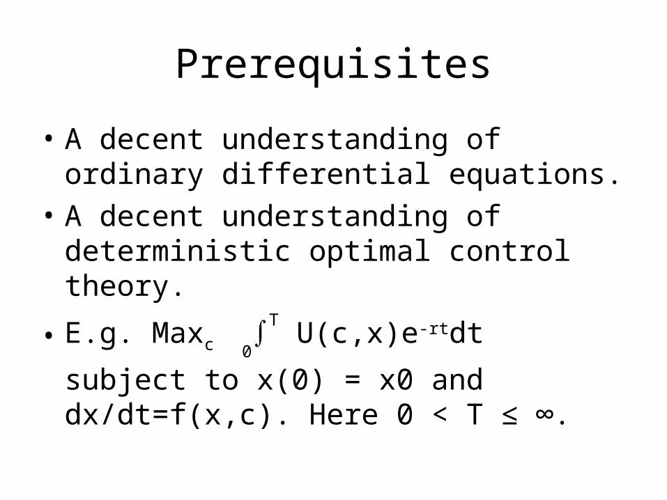
Prerequisites
• A decent understanding of ordinary differential equations.
• A decent understanding of deterministic optimal control theory.
• E.g. Maxc 0∫T U(c,x)e-rtdt subject to x(0) = x0
and dx/dt=f(x,c). Here 0 < T ≤ ∞.
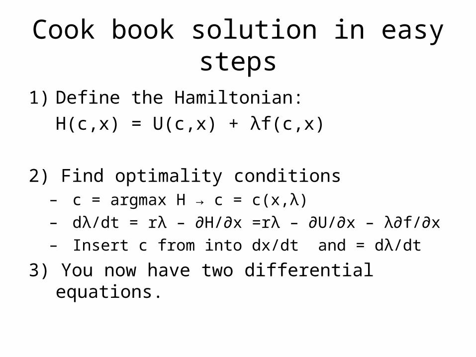
Cook book solution in easy steps
1) Define the Hamiltonian:
H(c,x) = U(c,x) + λf(c,x)
2) Find optimality conditions– c = argmax H → c = c(x,λ)– dλ/dt = rλ – ∂H/∂x =rλ – ∂U/∂x – λ∂f/∂x– Insert c from into dx/dt and = dλ/dt
3) You now have two differential equations.
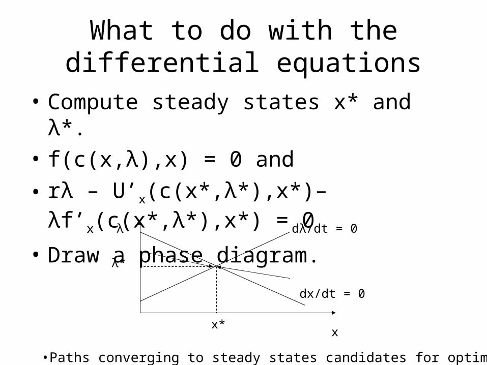
What to do with the differential equations
• Compute steady states x* and λ*.
• f(c(x,λ),x) = 0 and
• rλ – U’x(c(x*,λ*),x*)– λf’x(c(x*,λ*),x*) = 0
• Draw a phase diagram.
x
λ
dx/dt = 0
dλ/dt = 0
x*
λ*
•Paths converging to steady states candidates for optimal solution

Optimal Control cont’d
• The co-state λ(t) has an interesting economic interpretation.
• If somebody at time t gave you a present of 1 unit of x so that x(t) jumps to x(t) +1, then λ(t) is (roughly) the value of that present at time t.
• Entirely analogous to shadow prices in static theory.
• If T < ∞, then we have the transversality condition λ(t) = 0 if x(T) is free.

Transversality conditions for infinite Horizon problems
• The economic literature is full of flawed transversality conditions.
• The reason is that it is hard to find general conditions without using stuff like lim sup.
• For the purposes of this class we are satisfied if we can find at least one path where both the (current value) shadow price and the state variable converges to finite numbers.
• If T = ∞, then we really have a hard time with pinning down good transversality conditions. See Seierstad and Sydsæter (1987) for details.
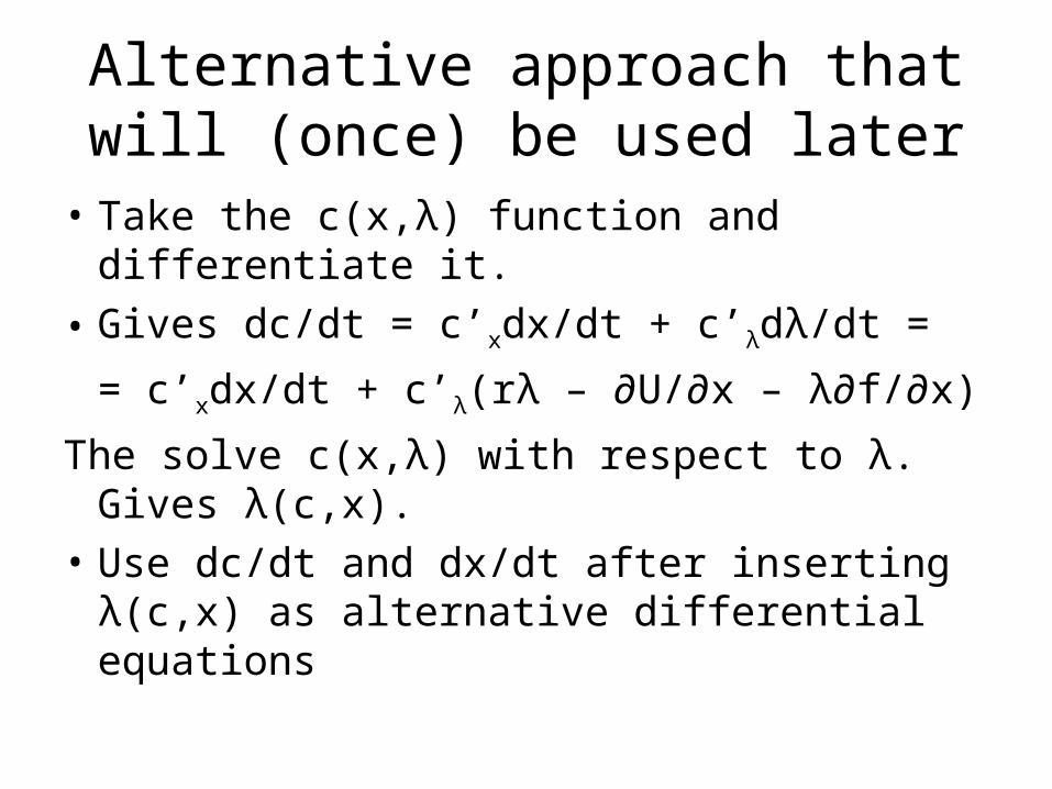
Alternative approach that will (once) be used later
• Take the c(x,λ) function and differentiate it.
• Gives dc/dt = c’xdx/dt + c’λdλ/dt =
= c’xdx/dt + c’λ(rλ – ∂U/∂x – λ∂f/∂x)
The solve c(x,λ) with respect to λ. Gives λ(c,x).
• Use dc/dt and dx/dt after inserting λ(c,x) as alternative differential equations
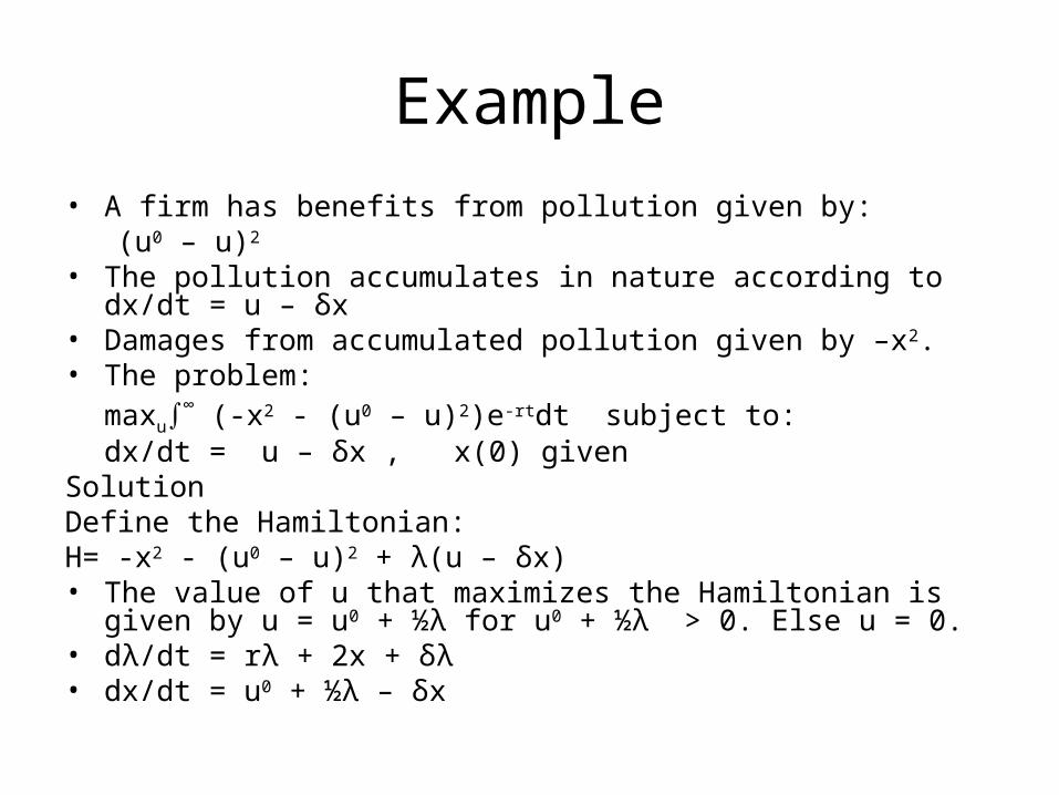
Example
• A firm has benefits from pollution given by: (u0 – u)2 • The pollution accumulates in nature according to dx/dt = u – δx • Damages from accumulated pollution given by –x2.• The problem:
maxu∫∞ (-x2 - (u0 – u)2)e-rtdt subject to:
dx/dt = u – δx , x(0) givenSolutionDefine the Hamiltonian:H= -x2 - (u0 – u)2 + λ(u – δx)• The value of u that maximizes the Hamiltonian is given by u = u0 + ½λ for
u0 + ½λ > 0. Else u = 0.• dλ/dt = rλ + 2x + δλ• dx/dt = u0 + ½λ – δx
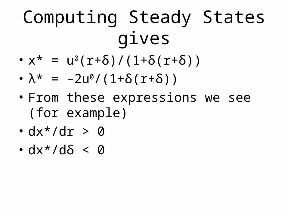
Computing Steady States gives
• x* = u0(r+δ)/(1+δ(r+δ))
• λ* = –2u0/(1+δ(r+δ))
• From these expressions we see (for example)
• dx*/dr > 0
• dx*/dδ < 0
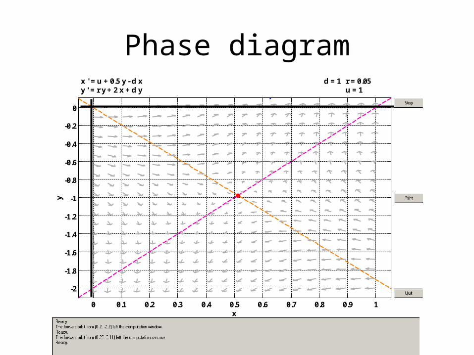
Phase diagramx ' = u + 0.5 y - d xy ' = r y + 2 x + d y
r = 0.05u = 1
d = 1
0 0.1 0.2 0.3 0.4 0.5 0.6 0.7 0.8 0.9 1
-2
-1.8
-1.6
-1.4
-1.2
-1
-0.8
-0.6
-0.4
-0.2
0
x
y

Phase diagram with pathsx ' = u + 0.5 y - d xy ' = r y + 2 x + d y
r = 0.05u = 1
d = 1
0 0.1 0.2 0.3 0.4 0.5 0.6 0.7 0.8 0.9 1
-2
-1.8
-1.6
-1.4
-1.2
-1
-0.8
-0.6
-0.4
-0.2
0
x
y

Phase diagram with paths and optimal paths for infinite horizon
x ' = u + 0.5 y - d xy ' = r y + 2 x + d y
r = 0.05u = 1
d = 1
0 0.1 0.2 0.3 0.4 0.5 0.6 0.7 0.8 0.9 1
-2
-1.8
-1.6
-1.4
-1.2
-1
-0.8
-0.6
-0.4
-0.2
0
x
y
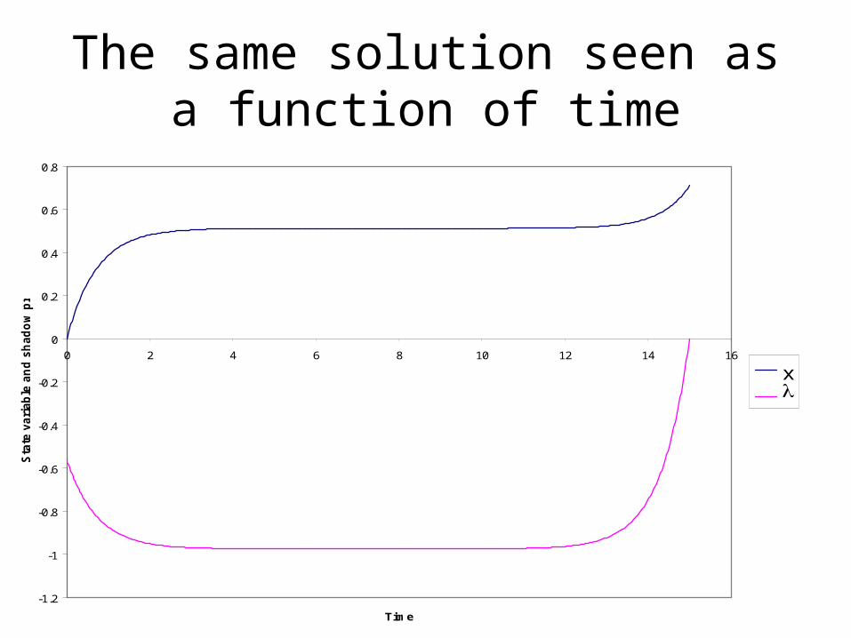
The same solution seen as a function of time
-1.2
-1
-0.8
-0.6
-0.4
-0.2
0
0.2
0.4
0.6
0.8
0 2 4 6 8 10 12 14 16
Time
Sta
te v
ari
ab
le a
nd
sh
ad
ow
pri
ce
xl
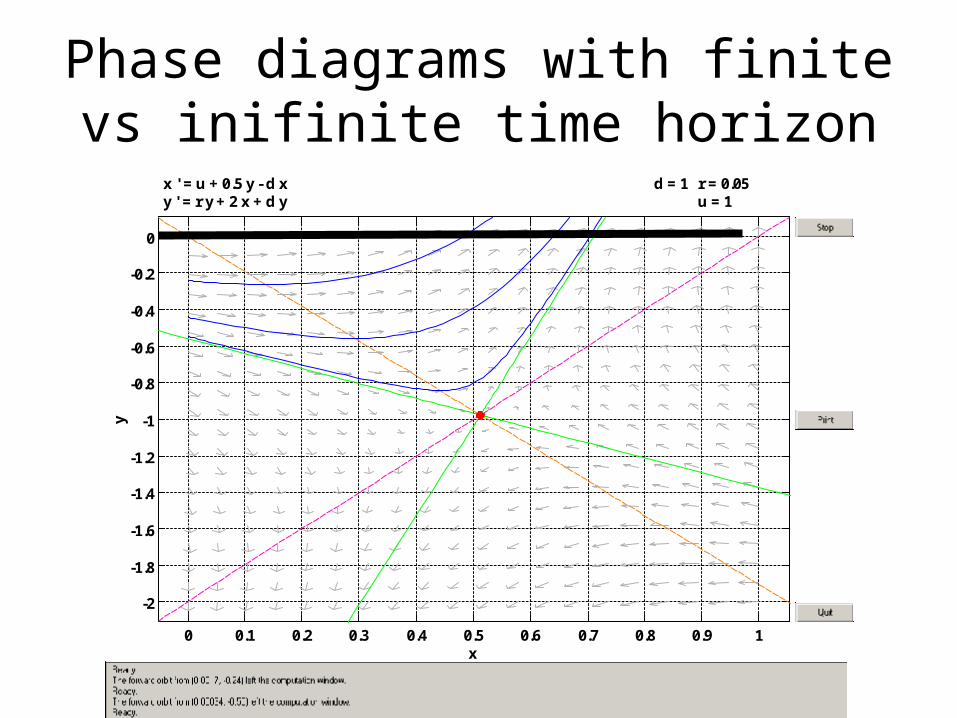
Phase diagrams with finite vs inifinite time horizon
x ' = u + 0.5 y - d xy ' = r y + 2 x + d y
r = 0.05u = 1
d = 1
0 0.1 0.2 0.3 0.4 0.5 0.6 0.7 0.8 0.9 1
-2
-1.8
-1.6
-1.4
-1.2
-1
-0.8
-0.6
-0.4
-0.2
0
x
y
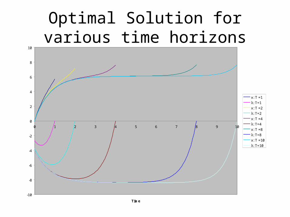
Optimal Solution for various time horizons
-10
-8
-6
-4
-2
0
2
4
6
8
10
0 1 2 3 4 5 6 7 8 9 10
Time
x: T =1
λ: T=1
x: T =2
λ: T=2
x: T =4
λ: T=4
x: T =8
λ: T=8
x: T =10
λ: T=10

Crucial insight
• If T is chosen sufficiently large, there will be some value t* such that the optimal solution for the infinite horizon problem and the optimal solution for the finite horizon problem will be numerically indistinguishable over the interval [0,t*]. This allows us to solve infinite horizon problems on the computer

Getting a deeper understanding of Optimal Control
• Some mathematical background: Boundary value problems. A general class of differential equations.
• Consider the problem dL/dt =λL, L(0) = L0. You should all know that the solution is: L0eλt.
• But what about this problem?:
dL/dt =λL, L(T) = LT
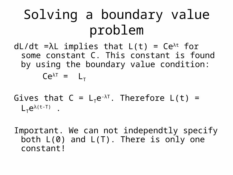
Solving a boundary value problem
dL/dt =λL implies that L(t) = Ceλt for some constant C. This constant is found by using the boundary value condition:
CeλT = LT
Gives that C = LTe-λT. Therefore L(t) = LTeλ(t-T) .
Important. We can not independtly specify both L(0) and L(T). There is only one constant!
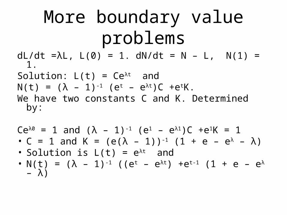
More boundary value problems
dL/dt =λL, L(0) = 1. dN/dt = N – L, N(1) = 1.Solution: L(t) = Ceλt and N(t) = (λ – 1)-1 (et – eλt)C +etK. We have two constants C and K. Determined by:
Ceλ0 = 1 and (λ – 1)-1 (e1 – eλ1)C +e1K = 1 • C = 1 and K = (e(λ – 1))-1 (1 + e – eλ – λ)• Solution is L(t) = eλt and • N(t) = (λ – 1)-1 ((et – eλt) +et-1 (1 + e – eλ – λ)

Why boundary value problems?
• The solution to an optimal control problem may be written as a boundary value problem. Best seen in finite time problems:
• max 0∫T U(c,x)e-rtdt subject to x(0) = x0 and
dx/dt=f(x,c). Here 0 < T< ∞. x(T) free.
• The maxmimum principle we know, but look at the transversality condition. λ(T)=0.

An even simpler example
Define the Hamiltonian:
H= -ax - ½(u0 – u)2 + λ(u – δx)
1. The value of u that maximizes the Hamiltonian is given by u = u0 + ½λ for u0 + ½λ > 0. Else u = 0.
2. dλ/dt = rλ + a + δλ
3. dx/dt = u0 + ½λ – δx
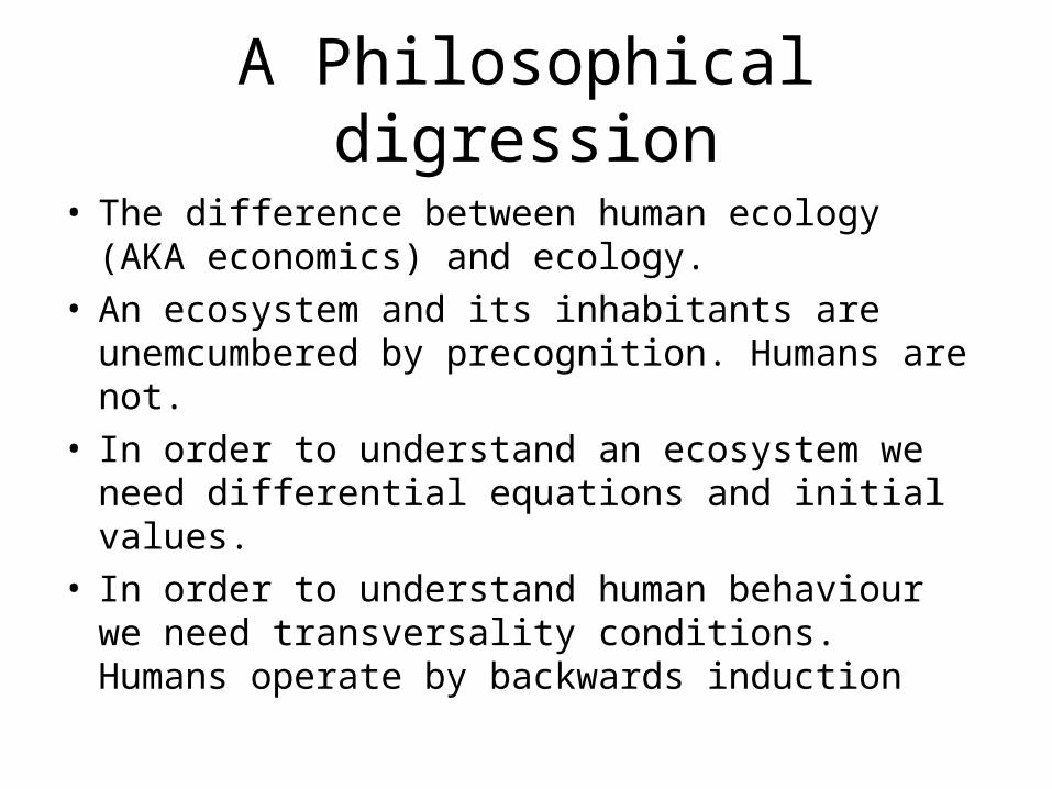
A Philosophical digression
• The difference between human ecology (AKA economics) and ecology.
• An ecosystem and its inhabitants are unemcumbered by precognition. Humans are not.
• In order to understand an ecosystem we need differential equations and initial values.
• In order to understand human behaviour we need transversality conditions. Humans operate by backwards induction

Numerical methods
• Standard Optimal Control Problems in the literature do the following:– Find explicit solutions. Works for very few
problems. – Phase diagram. Only works for problems with one
state variable.– Steady state analysis. May be hard to do for some
problems. Some times steay states are uninteresting
• Alternative: Numerical analysis

Numerical Methods in finite time - Shooting
• The basic problem; The Maximum Principle gives us a set of differential equations.
• An optimal solution must start with the known and correct initial value of x(0). It must also start with an unknown correct value of λ(0) such that λ(T) = 0.
• Alternatively if x(T) is given, λ(0) must start from a value so that those constraint holds.
• The fundamental problem: Solve a rather complicated equation to find λ(0).
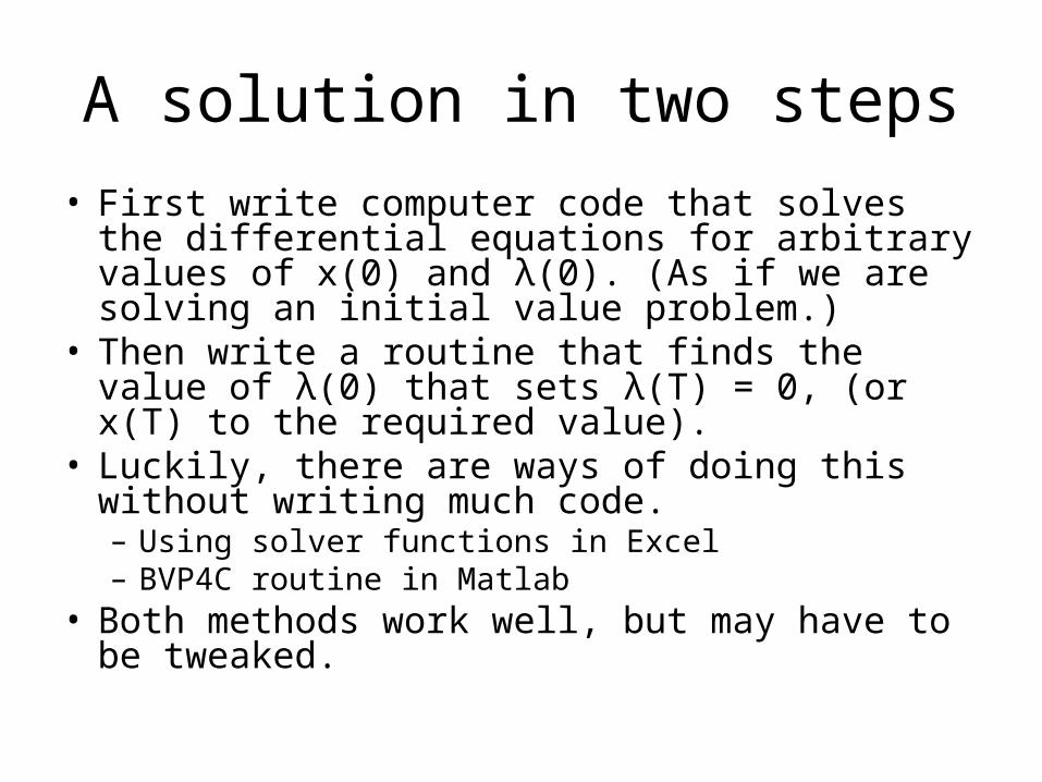
A solution in two steps
• First write computer code that solves the differential equations for arbitrary values of x(0) and λ(0). (As if we are solving an initial value problem.)
• Then write a routine that finds the value of λ(0) that sets λ(T) = 0, (or x(T) to the required value).
• Luckily, there are ways of doing this without writing much code.– Using solver functions in Excel– BVP4C routine in Matlab
• Both methods work well, but may have to be tweaked.

Step 1. The 4th order Runge – Kutta Method
• General formulation. For an OC problem the vector y = [x, λ].
• Let dy/dt = f(t, y). Let h be a small number. Then y(t) is usually well approximated by the following sequence:
• y(t+h) = y(t) +(h/6)×(k1 + 2k2 + 2k3 + k4)
k1= f(t, y(t)), k2=f(t + h/2, y(t) +hk1/2)
k3=f(t + h/2, y(t) +hk2/2), k4= f(t + h, y(t) + hk3)

Starting Example
• Let dy/dt =y (1- y), y(0) = ½. The solution to this differential equation :
• y(t) = Exp(t)/(1 + Exp(t))
• No difference
whatsoever!
0
0.2
0.4
0.6
0.8
1
1.2
0 2 4 6 8 10 12
Time
Runge Kutta
True Solution
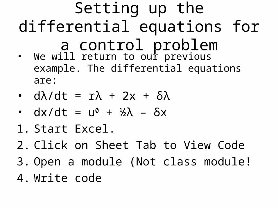
Setting up the differential equations for a control problem
• We will return to our previous example. The differential equations are:
• dλ/dt = rλ + 2x + δλ
• dx/dt = u0 + ½λ – δx
1. Start Excel.
2. Click on Sheet Tab to View Code
3. Open a module (Not class module!
4. Write code

May look like this:

Implemenent Runge Kutta in Spreadsheet.
• Time to load spread sheet Small Optimal Control Example

Step 2 – Finding λ(0)
• May in principle be done by programming some suitable search algorithm.
• We are going to let Excel take care of it.• Two ways of doing this
– Goal Seek Function. Slow, robust, only handles problems with one state variable
– The Solver. Fast, will stop if the algorithm encounters errors, Handles a large number state variables.
• Let’s do it.
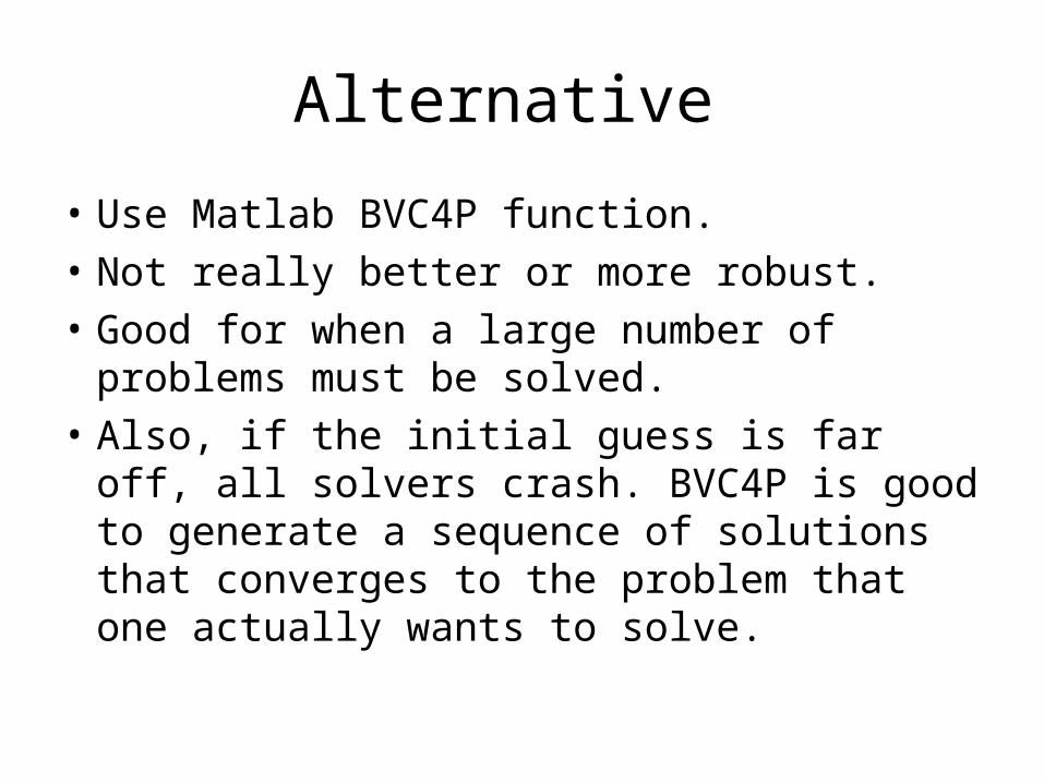
Alternative
• Use Matlab BVC4P function.
• Not really better or more robust.
• Good for when a large number of problems must be solved.
• Also, if the initial guess is far off, all solvers crash. BVC4P is good to generate a sequence of solutions that converges to the problem that one actually wants to solve.
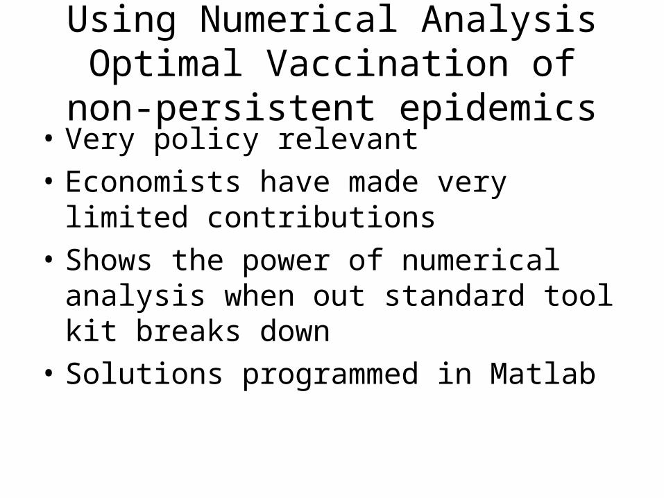
Using Numerical Analysis Optimal Vaccination of non-persistent
epidemics• Very policy relevant
• Economists have made very limited contributions
• Shows the power of numerical analysis when out standard tool kit breaks down
• Solutions programmed in Matlab
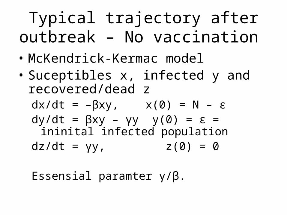
Typical trajectory after outbreak – No vaccination
• McKendrick-Kermac model• Suceptibles x, infected y and recovered/dead z
dx/dt = –βxy, x(0) = N – εdy/dt = βxy – γy y(0) = ε = ininital infected
populationdz/dt = γy, z(0) = 0
Essensial paramter γ/β.
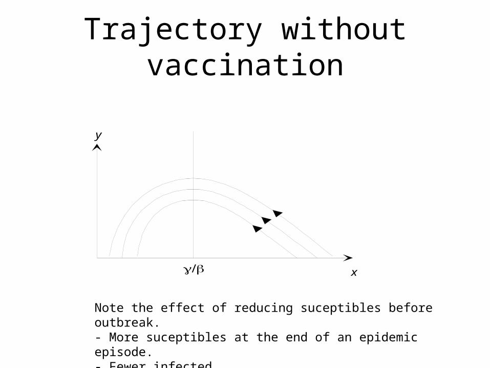
Trajectory without vaccination
x
y
Note the effect of reducing suceptibles before outbreak.- More suceptibles at the end of an epidemic episode.- Fewer infected

Model with vaccination
• Individuals may be vaccinated u.dx/dt = –βxy – u, x(0) = N – εdy/dt = βxy – γy y(0) = ε = ininital infected dz/dt = γy + u, z(0) = 0
Objective function:∫(-wy - ½cu2)e-rtdt K is the cost of disease .½cu2 is the cost of vaccination
Must be solved numerically. Standard tools of optimal control useless.

Optimal vaccination - Low cost of disease (w)

Optimal vaccination - High cost of disease (w)
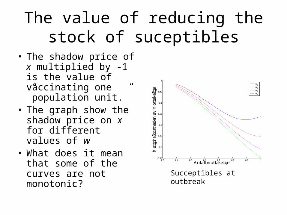
The value of reducing the stock of suceptibles
• The shadow price of x multiplied by -1 is the value of vaccinating one ”population unit.”
• The graph show the shadow price on x for different values of w
• What does it mean that some of the curves are not monotonic?
0.3 0.4 0.5 0.6 0.7 0.8 0.9 1-0.35
-0.3
-0.25
-0.2
-0.15
-0.1
-0.05
0
Antall mottakelige
Mar
gina
lkos
tnad
en a
v m
otta
kelig
e
w2
w4
w1
w3
Succeptibles at outbreak
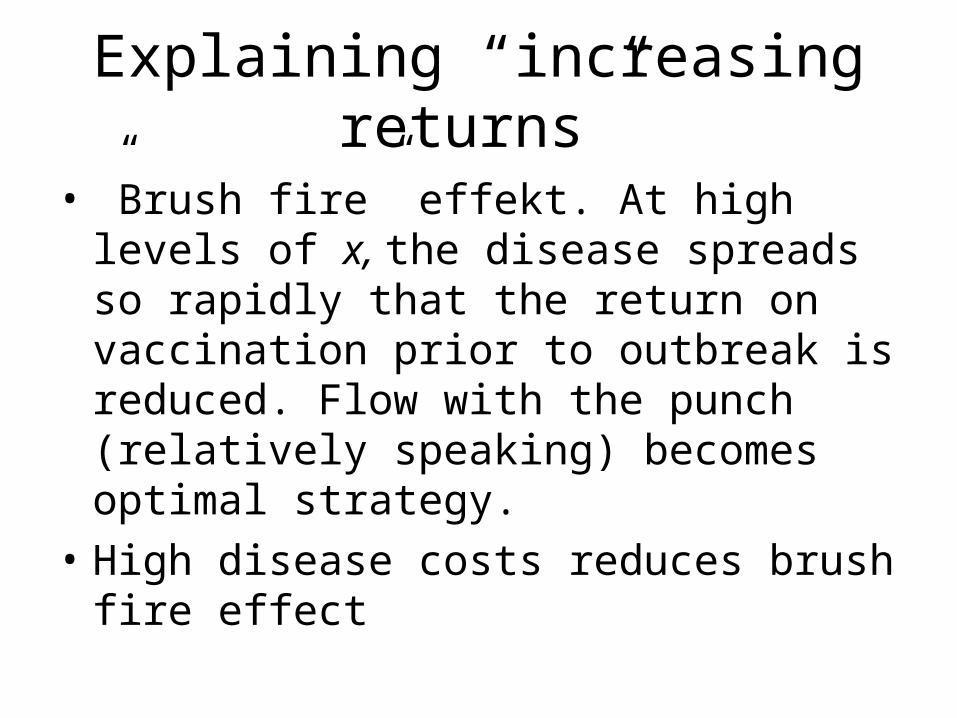
Explaining “increasing returns”
• ”Brush fire” effekt. At high levels of x, the disease spreads so rapidly that the return on vaccination prior to outbreak is reduced. Flow with the punch (relatively speaking) becomes optimal strategy.
• High disease costs reduces brush fire effect

New Section Multiple Equilibria
• Many systems exhibit non-linear dynamics. May or may represent a technical challenge
• Here we look at convexo-concave differential equations.
• Important to note that systems that naturally exhibit multiple equilibria may not do so when controlled optimally
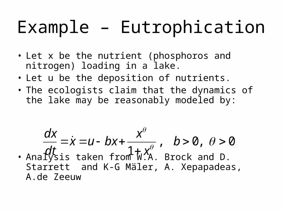
Example – Eutrophication
• Let x be the nutrient (phosphoros and nitrogen) loading in a lake.
• Let u be the deposition of nutrients.• The ecologists claim that the dynamics of the lake
may be reasonably modeled by:
• Analysis taken from W.A. Brock and D. Starrett and K-G Mäler, A. Xepapadeas, A.de Zeeuw
0,0,1
bx
xbxux
dt
dx
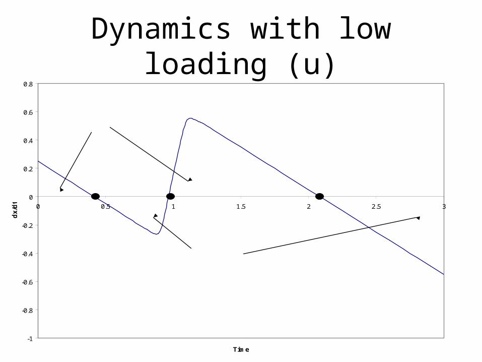
Dynamics with low loading (u)
-1
-0.8
-0.6
-0.4
-0.2
0
0.2
0.4
0.6
0.8
0 0.5 1 1.5 2 2.5 3
Time
dx/d
t
Positive derivative
Negative derivative
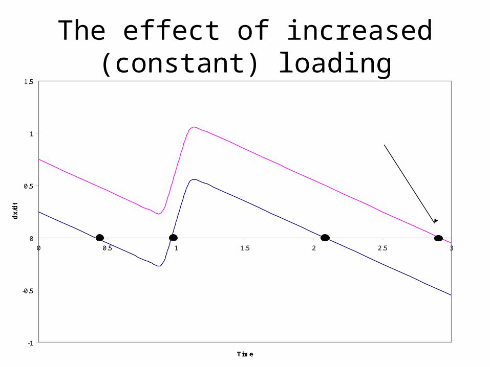
The effect of increased (constant) loading
-1
-0.5
0
0.5
1
1.5
0 0.5 1 1.5 2 2.5 3
Time
dx/d
t
New unique steady state.Global attractor
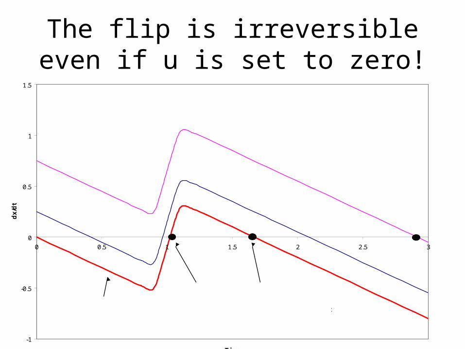
The flip is irreversible even if u is set to zero!
-1
-0.5
0
0.5
1
1.5
0 0.5 1 1.5 2 2.5 3
Time
dx/d
t
Point of no return
"Best" long run state of nature if we go past point of no rerurn
Zero loading equation

Management
• For economic analysis we need some evaluation of consequences.
• Instantaneous benefits from nutrient use given by ½ln(u)
• Instantaneous damages from eutrophication given by –cx2.
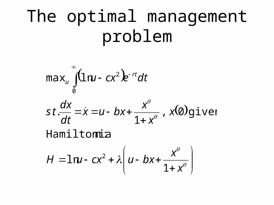
The optimal management problem
lx
xbxucxuH
xx
xbxux
dt
dxts
dtecxu rtu
1ln
:nHamiltonia
given 0,1
..
lnmax
2
0
2

Optimality Conditions
l
lll
l
x
xbxx
x
xbcxr
uHu
1
1
12
1maxarg
2
1

Transforming into equations in (u,x) space
space ,in equations
aldifferentiget we1
ith Together w
12
:gives for expression theinto and 1
Insert
and 1
22
2
uxx
xbxux
xx
xurubucxuu
u u
uu
ll
lll
Draw differential equations
• We proceed to draw a phase diagram in (x,u) space.
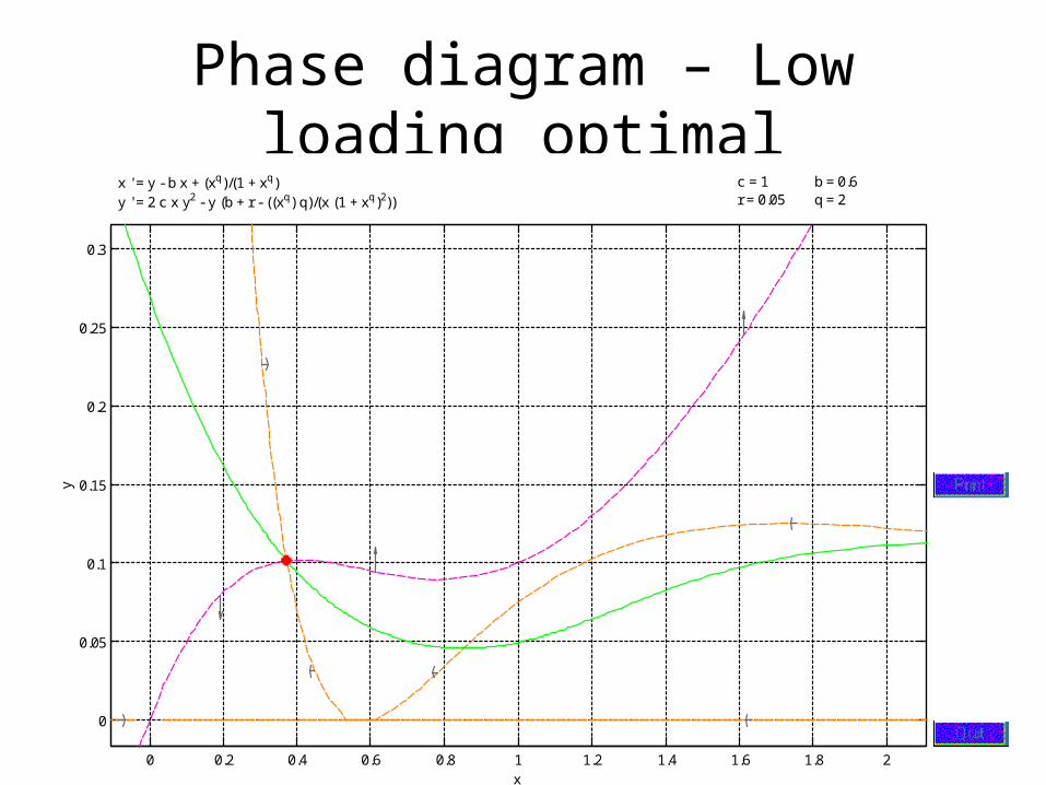
Phase diagram – Low loading optimalx ' = y - b x + (xq)/(1 + xq) y ' = 2 c x y2 - y (b + r - ((xq) q)/(x (1 + xq)2))
b = 0.6q = 2
c = 1r = 0.05
0 0.2 0.4 0.6 0.8 1 1.2 1.4 1.6 1.8 2
0
0.05
0.1
0.15
0.2
0.25
0.3
x
y

Phase diagram – High loading optimalx ' = y - b x + (xq)/(1 + xq) y ' = 2 c x y2 - y (b + r - ((xq) q)/(x (1 + xq)2))
b = 0.6q = 2
c = 0.1r = 0.15
0 0.5 1 1.5 2 2.5 3 3.5 4 4.5 5
0
0.5
1
1.5
2
2.5
3
3.5
4
4.5
5
x
y
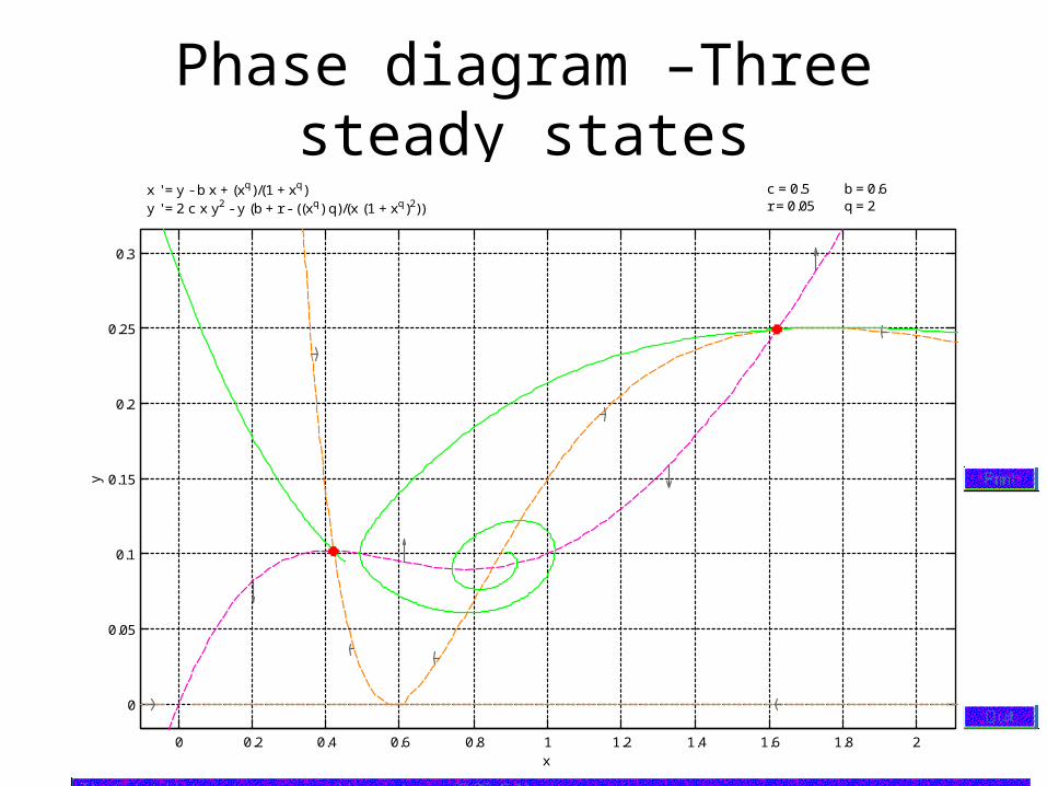
Phase diagram –Three steady statesx ' = y - b x + (xq)/(1 + xq) y ' = 2 c x y2 - y (b + r - ((xq) q)/(x (1 + xq)2))
b = 0.6q = 2
c = 0.5r = 0.05
0 0.2 0.4 0.6 0.8 1 1.2 1.4 1.6 1.8 2
0
0.05
0.1
0.15
0.2
0.25
0.3
x
y
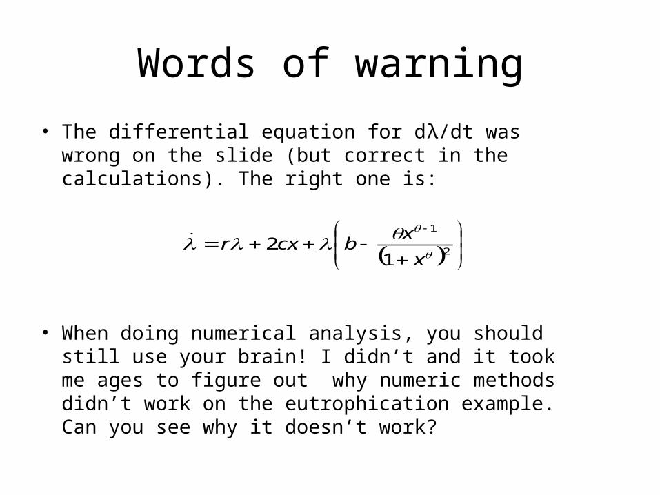
Words of warning
• The differential equation for dλ/dt was wrong on the slide (but correct in the calculations). The right one is:
• When doing numerical analysis, you should still use your brain! I didn’t and it took me ages to figure out why numeric methods didn’t work on the eutrophication example. Can you see why it doesn’t work?
2
1
12
lllx
xbcxr

Modify the Eutrophication model
lx
xbxucxuH
xx
xbxux
dt
dxts
dtecxuu rtu
1ln
:nHamiltonia
given 0,1
..
2
1max
2
0
220

High cost of eutrophication – Only oligotrophic Equilibrium
x ' = 5 + y - b x + (xq)/(1 + xq) y ' = 2 c x + (b + r - ((x(q - 1)) q)/((1 + xq)2)) y
b = 0.6q = 2
c = 0.8r = 0.15
0 0.5 1 1.5 2 2.5 3
-8
-7
-6
-5
-4
-3
-2
-1
0
x
y

Intermediate cost – The Skiba story
x ' = 5 + y - b x + (xq)/(1 + xq) y ' = 2 c x + (b + r - ((x(q - 1)) q)/((1 + xq)2)) y
b = 0.6q = 2
c = 0.7r = 0.15
0 0.5 1 1.5 2 2.5
-7
-6
-5
-4
-3
-2
-1
0
x
y

High cost of eutrophication
x ' = 5 + y - b x + (xq)/(1 + xq) y ' = 2 c x + (b + r - ((x(q - 1)) q)/((1 + xq)2)) y
b = 0.6q = 2
c = 0.5r = 0.15
0 0.5 1 1.5 2 2.5 3 3.5
-8
-7
-6
-5
-4
-3
-2
-1
0
x
y
A
B
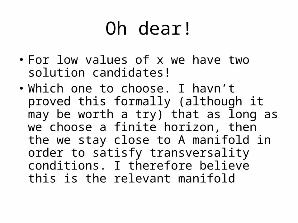
Oh dear!
• For low values of x we have two solution candidates!
• Which one to choose. I havn’t proved this formally (although it may be worth a try) that as long as we choose a finite horizon, then the we stay close to A manifold in order to satisfy transversality conditions. I therefore believe this is the relevant manifold

Genetic Management
• Many people are concerned with biodiversity.• I am, for various reasons, not. But I am
concerned about outcomes.• Harvesting living resources leads to
evolutionary genetic selection.• How to regulate this?• Also, an example of non-standard analysis.


Objective
Construct a bioeconomic model where we analyze the effect of selective harvesting on genetic frequency for one specific gene in terms of the socially optimal long-term management of the resource. This object is determined solely through the profits generated by harvesting

Genetic Dynamics
• Standard model of Mendelian genetics• Two alleles, A and a of the same gene. • The homozygotes AA and the heterozygote Aa are of
phenotype G (for good) • The homozygote aa are of phenotype B (for bad)• The frequency of a is q. (q = 1 is bad. q = 0 is good.)• Only individuals of type G are of commercial
interest, and harvesting is totally selective
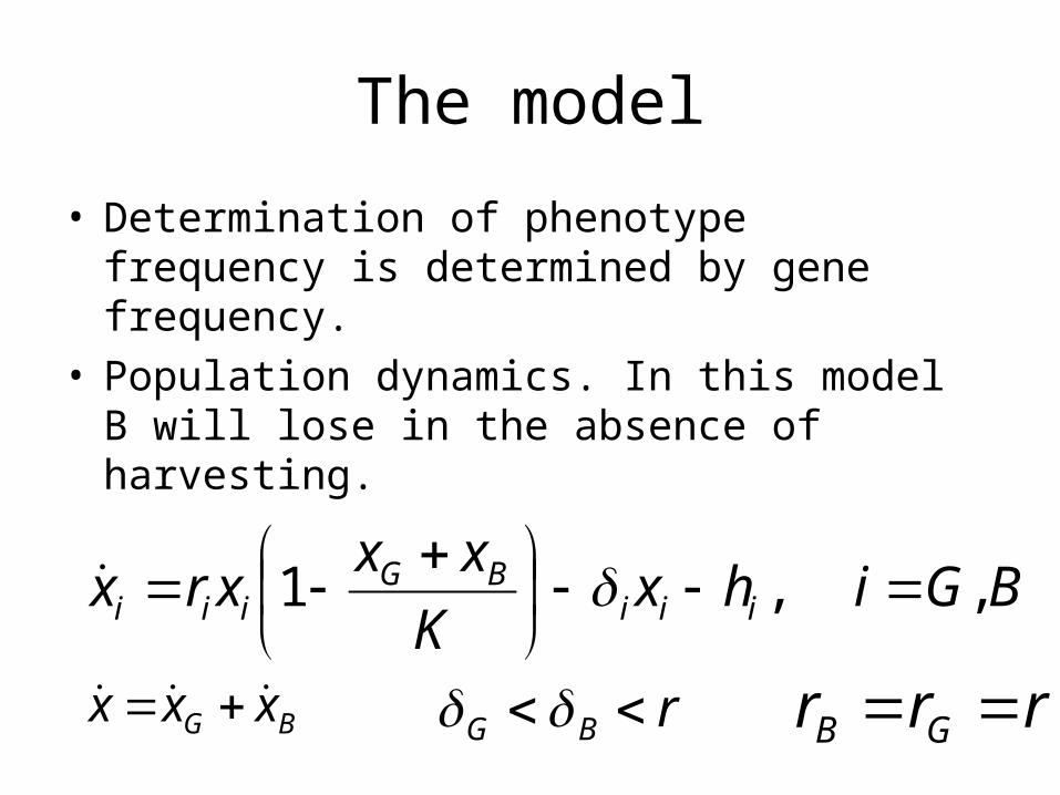
The model
• Determination of phenotype frequency is determined by gene frequency.
• Population dynamics. In this model B will lose in the absence of harvesting.
BGihxK
xxxrx iii
BGiii , ,1
BG xxx rBG rrr GB
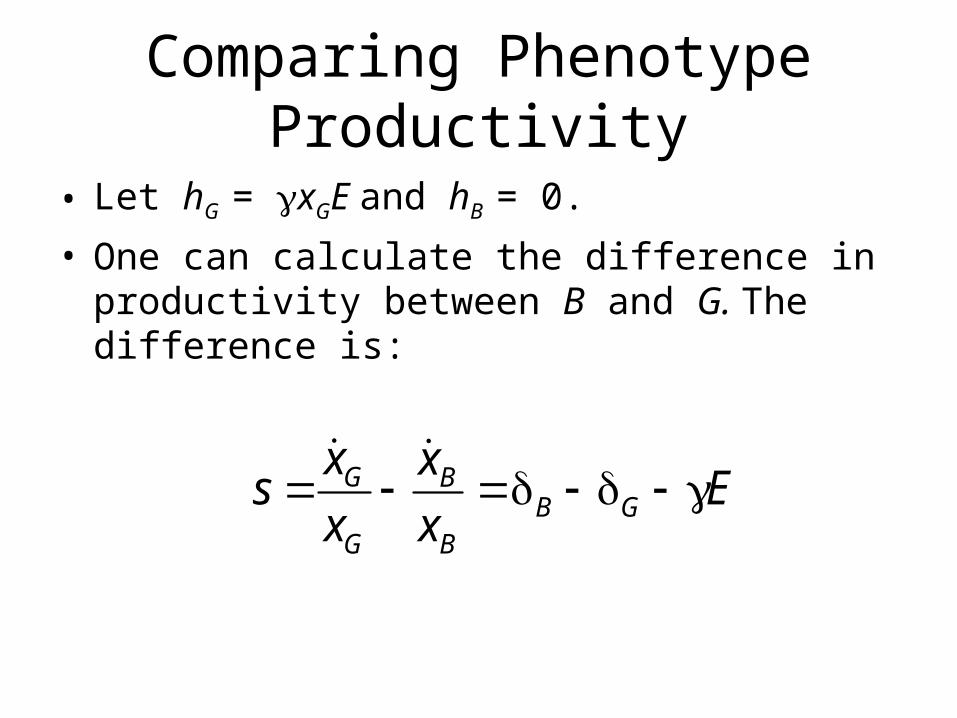
Comparing Phenotype Productivity
• Let hG = xGE and hB = 0.
• One can calculate the difference in productivity between B and G. The difference is:
G BB G
G B
x xs E
x x
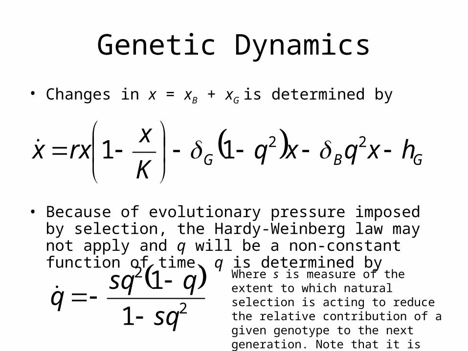
Genetic Dynamics
• Changes in x = xB + xG is determined by
• Because of evolutionary pressure imposed by selection, the Hardy-Weinberg law may not apply and q will be a non-constant function of time. q is determined by
GBG hxqxqK
xrxx
2211
2
2
1
1
sq
qsqq
Where s is measure of the extent to which natural selection is acting to reduce the relative contribution of a given genotype to the next generation. Note that it is also the productivity difference!
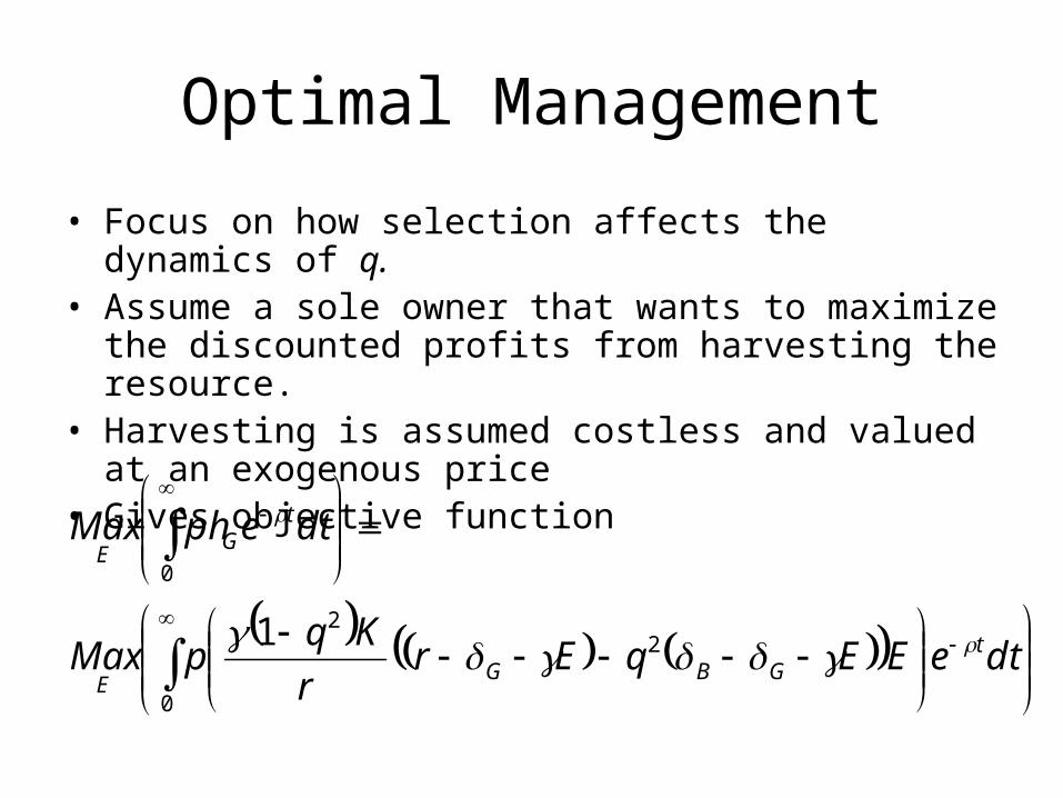
Optimal Management
• Focus on how selection affects the dynamics of q.• Assume a sole owner that wants to maximize the discounted
profits from harvesting the resource. • Harvesting is assumed costless and valued at an exogenous
price • Gives objective function
0
22
0
1dteEEqEr
r
KqpMax
dtephMax
tGBG
E
tG
E

Optimization Problem
0
22
0
1dteEEqEr
r
KqpMax
dtephMax
tGBG
E
tG
E
2
2
1
1
qE
Eqqq
GB
GB
s.t
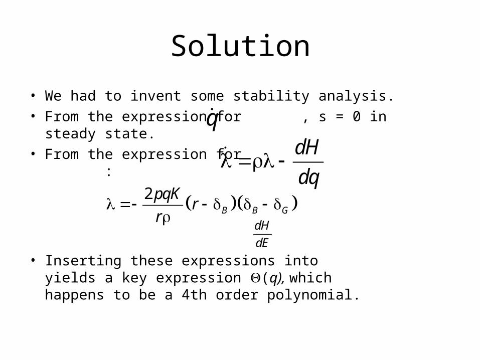
Solution
• We had to invent some stability analysis.
• From the expression for , s = 0 in steady state.
• From the expression for :
• Inserting these expressions into yields a key expression (q), which happens to be a 4th order polynomial.
qdH
dql l
2B B G
pqKr
rl
dH
dE
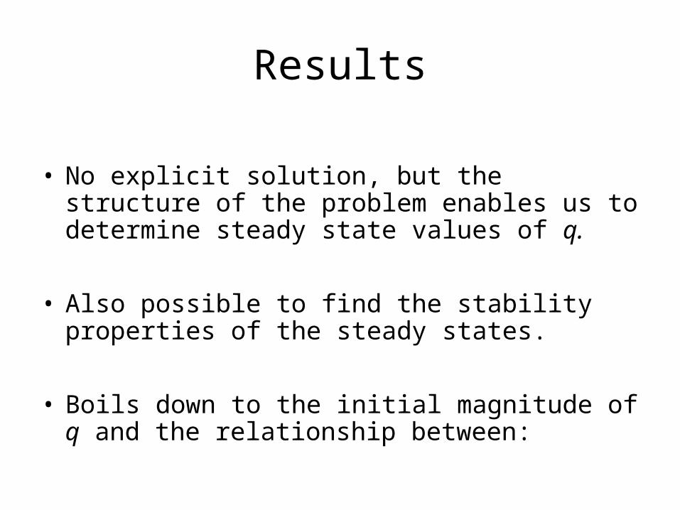
Results
• No explicit solution, but the structure of the problem enables us to determine steady state values of q.
• Also possible to find the stability properties of the steady states.
• Boils down to the initial magnitude of q and the relationship between:
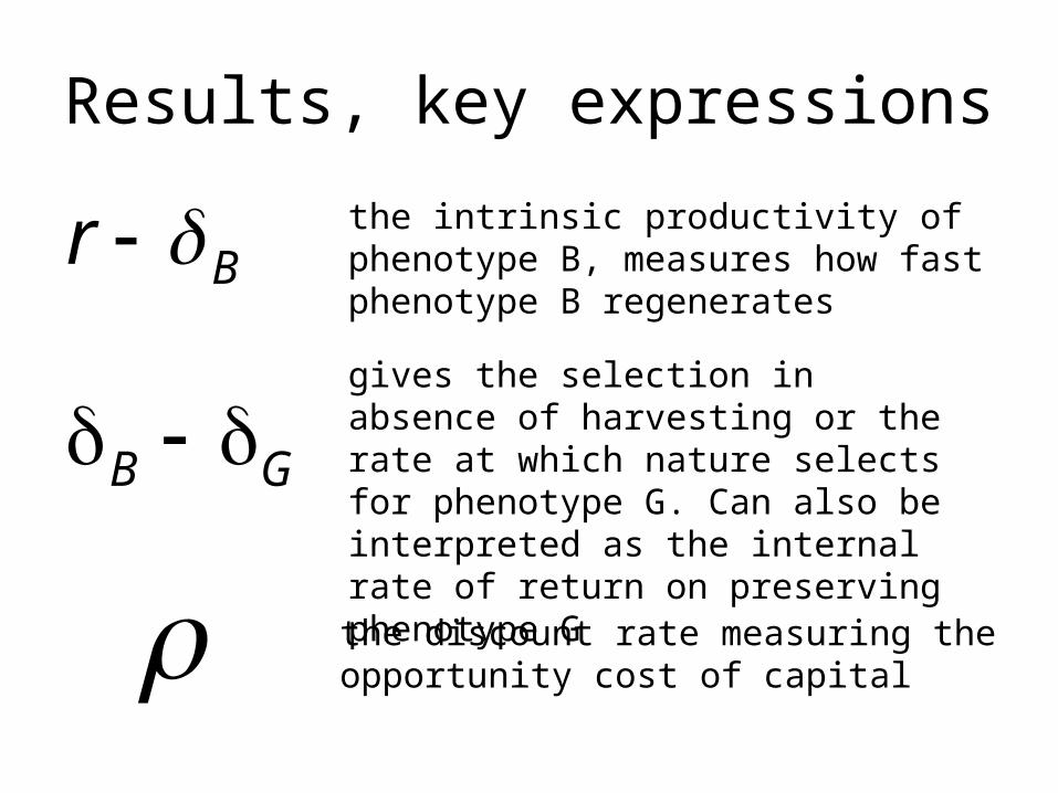
Results, key expressions
Br
B G
the intrinsic productivity of phenotype B, measures how fast phenotype B regenerates
gives the selection in absence of harvesting or the rate at which nature selects for phenotype G. Can also be interpreted as the internal rate of return on preserving phenotype G
the discount rate measuring the opportunity cost of capital
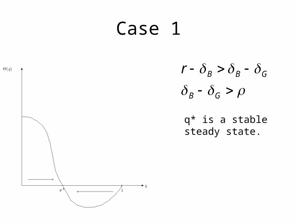
Case 1
GB
GBBr
q* is a stable steady state.
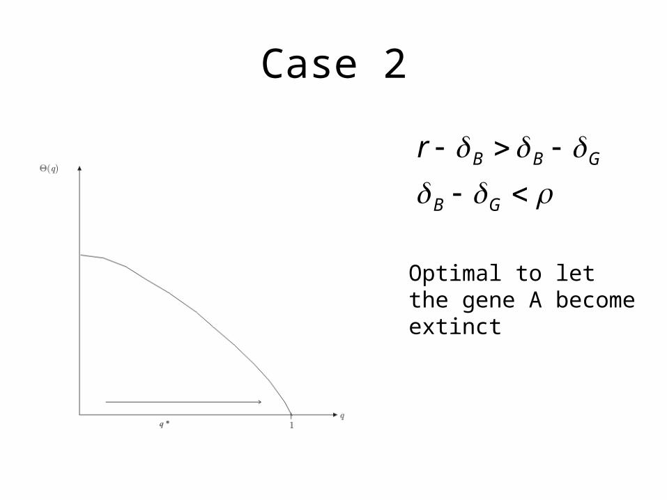
Case 2
GB
GBBr
Optimal to let the gene A become extinct

Case 3a
GB
GBBr
Optimal to let the gene a become extinct
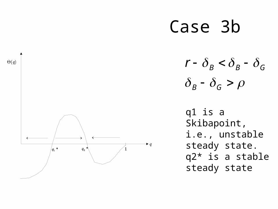
Case 3b
GB
GBBr
q1 is a Skibapoint, i.e., unstable steady state. q2* is a stable steady state
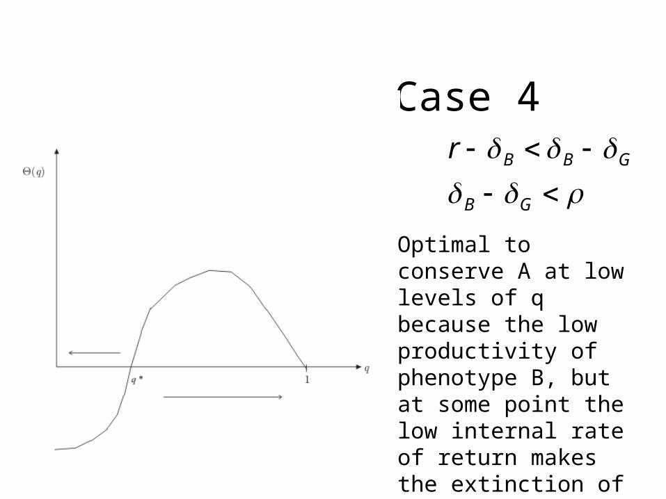
Case 4
GB
GBBr
Optimal to conserve A at low levels of q because the low productivity of phenotype B, but at some point the low internal rate of return makes the extinction of phenotype G optimal
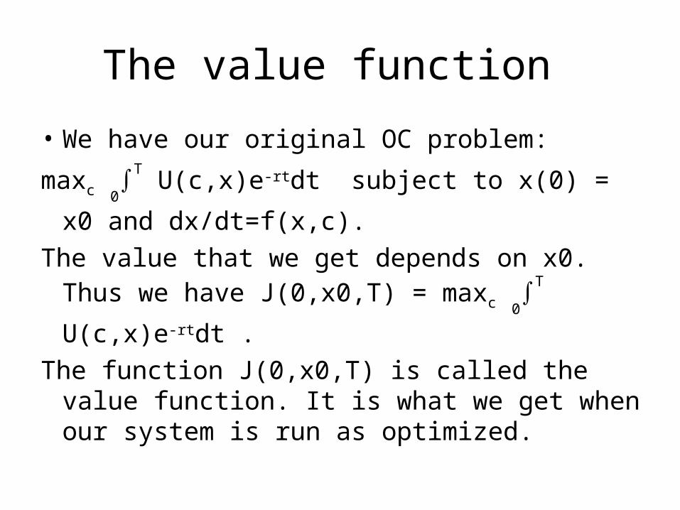
The value function
• We have our original OC problem:
maxc 0∫T U(c,x)e-rtdt subject to x(0) = x0 and
dx/dt=f(x,c).
The value that we get depends on x0. Thus we have J(0,x0,T) = maxc 0
∫T U(c,x)e-rtdt .
The function J(0,x0,T) is called the value function. It is what we get when our system is run as optimized.
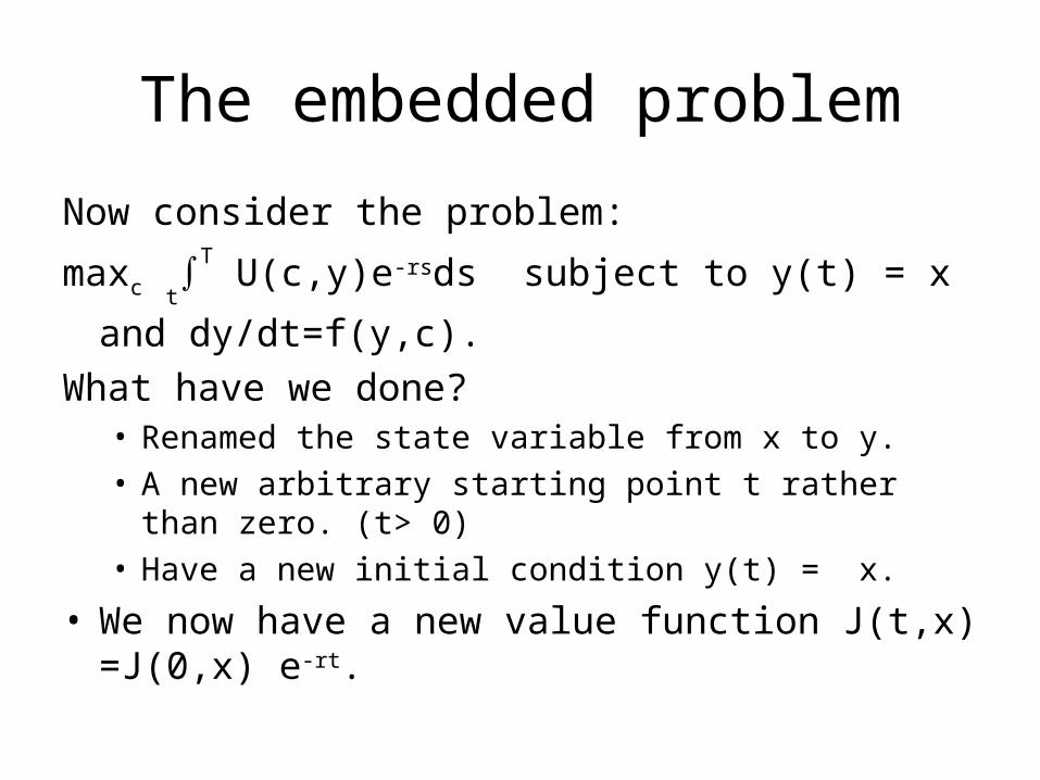
The embedded problem
Now consider the problem:
maxc t∫T U(c,y)e-rsds subject to y(t) = x and dy/dt=f(y,c).
What have we done?• Renamed the state variable from x to y.
• A new arbitrary starting point t rather than zero. (t> 0)
• Have a new initial condition y(t) = x.
• We now have a new value function J(t,x) =J(0,x) e-rt.
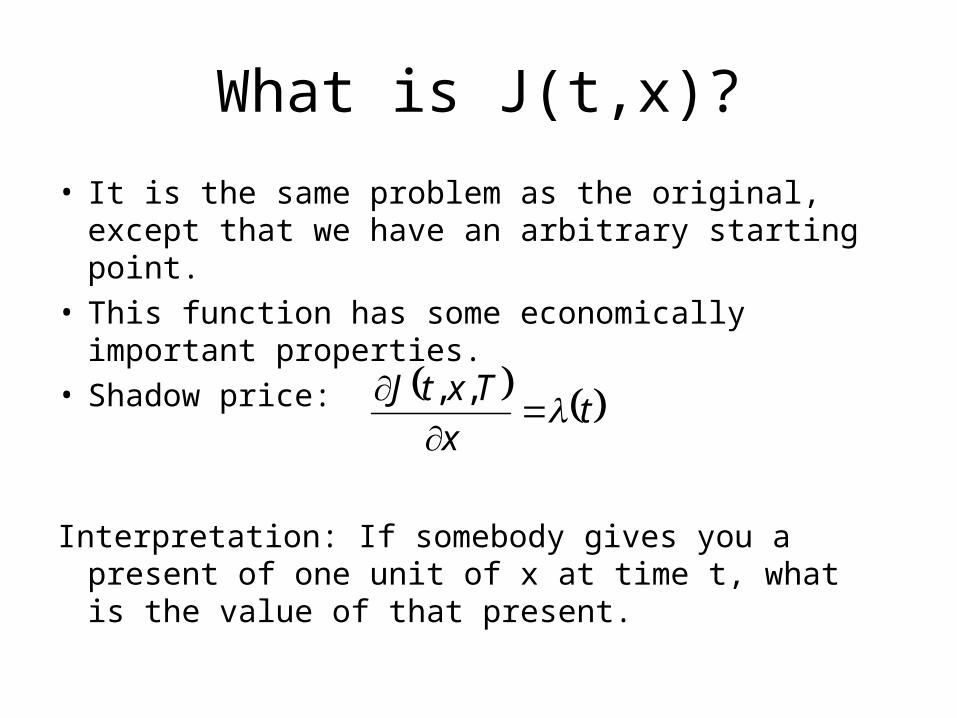
What is J(t,x)?
• It is the same problem as the original, except that we have an arbitrary starting point.
• This function has some economically important properties.
• Shadow price:
Interpretation: If somebody gives you a present of one unit of x at time t, what is the value of that present.
tx
TxtJ l
,,
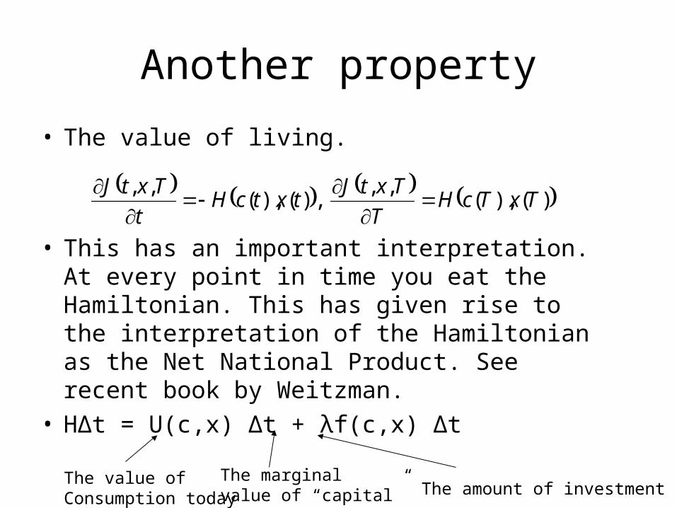
Another property
• The value of living.
• This has an important interpretation. At every point in time you eat the Hamiltonian. This has given rise to the interpretation of the Hamiltonian as the Net National Product. See recent book by Weitzman.
• HΔt = U(c,x) Δt + λf(c,x) Δt
)(),(,,
,)(),(,,
TxTcHT
TxtJtxtcH
t
TxtJ
The value of Consumption today
The marginal value of “capital” The amount of investment
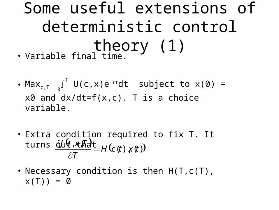
Some useful extensions of deterministic control theory (1)
• Variable final time.
• Maxc,T 0∫T U(c,x)e-rtdt subject to x(0) = x0 and
dx/dt=f(x,c). T is a choice variable.
• Extra condition required to fix T. It turns out that
• Necessary condition is then H(T,c(T), x(T)) = 0
)(),(,,
txtcHT
TxtJ
Very simple example
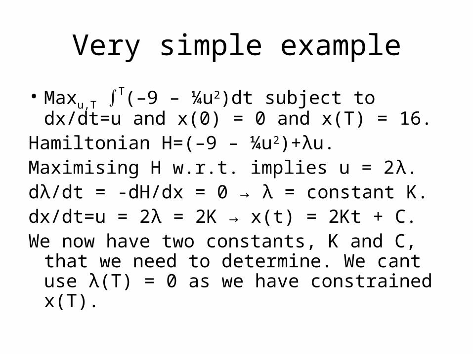
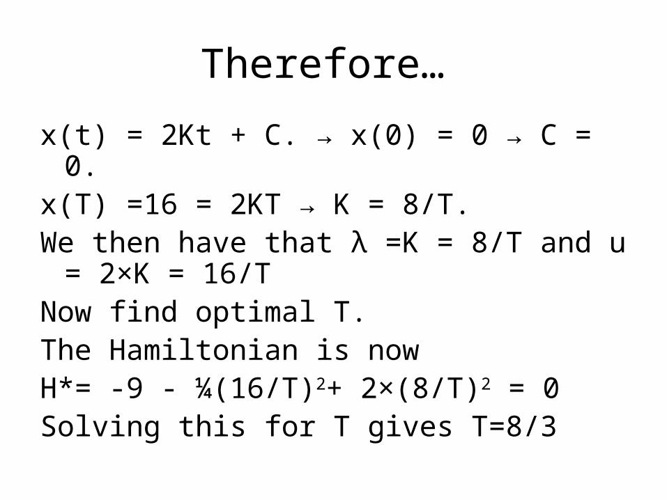
• Maxu,T ∫T(–9 – ¼u2)dt subject to dx/dt=u and x(0) = 0 and x(T) = 16.
Hamiltonian H=(–9 – ¼u2)+λu.Maximising H w.r.t. implies u = 2λ.dλ/dt = -dH/dx = 0 → λ = constant K.dx/dt=u = 2λ = 2K → x(t) = 2Kt + C.We now have two constants, K and C, that we
need to determine. We cant use λ(T) = 0 as we have constrained x(T).
Therefore…
x(t) = 2Kt + C. → x(0) = 0 → C = 0.x(T) =16 = 2KT → K = 8/T.We then have that λ =K = 8/T and u = 2×K =
16/TNow find optimal T.The Hamiltonian is now H*= -9 - ¼(16/T)2+ 2×(8/T)2 = 0Solving this for T gives T=8/3

Some useful extensions of deterministic control theory (2)
• Scrap value problems - a complicated problem finite horizon problem.
• E.g. Maxc,T 0∫T U(c,x)e-rtdt +S(x(T)) e-rT.
subject to x(0) = x0 and dx/dt=f(x,c). • Conditions:• The same conditions on c and λ. Different
transversality conditions:• λ(T) = S’(x(T)) e-rT. U(c,x)e-rt + λf(x,c) = r
S(x(T)) e-rT .

A closer look at these conditions
• Why are these conditions not surprising?• λ(T) = S’(x(T)). Says that the shadow price of x
should be continuous.
• U(c,x) + λf(x,c) = r S(x(T)) . Says that the change in utility from continuing one more unit of time should be the same as the loss from not cashing in on the scrap value. Remember that U(c,x)e-rT + λe-rTf(x,c) = J’(T,x).

Load Excel file

Deterministic Threshold Problems Irreversible case.
• A threshold is here defined to be some curve in state space such that crossing this curve leads to a discrete jump in state-variables.
• Preliminary observation; if the location of the threshold is known one can choose to cross the threshold or not cross the threshold.
• An irreversible threshold effect can be modeled as a scrap value problem with endogenous time horizon
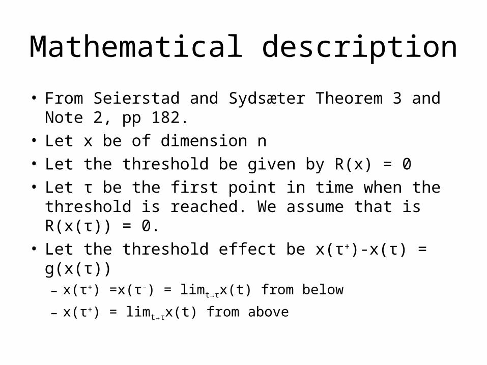
Mathematical description
• From Seierstad and Sydsæter Theorem 3 and Note 2, pp 182.
• Let x be of dimension n• Let the threshold be given by R(x) = 0• Let τ be the first point in time when the threshold is
reached. We assume that is R(x(τ)) = 0.• Let the threshold effect be x(τ+)-x(τ) = g(x(τ))
– x(τ+) =x(τ-) = limt→τx(t) from below
– x(τ+) = limt→τx(t) from above
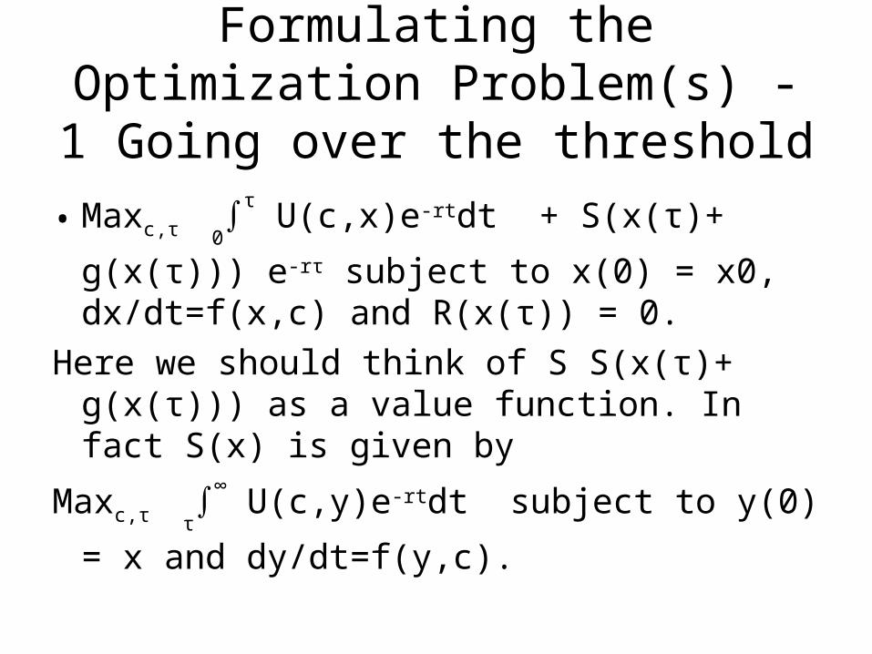
Formulating the Optimization Problem(s) - 1 Going over the
threshold
• Maxc,τ 0∫τ U(c,x)e-rtdt + S(x(τ)+ g(x(τ))) e-rτ
subject to x(0) = x0, dx/dt=f(x,c) and R(x(τ)) = 0.
Here we should think of S S(x(τ)+ g(x(τ))) as a value function. In fact S(x) is given by
Maxc,τ τ∫∞ U(c,y)e-rtdt subject to y(0) = x and
dy/dt=f(y,c).
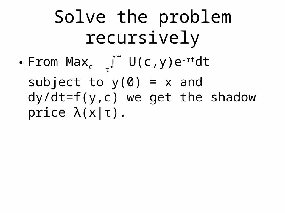
Solve the problem recursively
• From Maxc τ∫∞ U(c,y)e-rtdt subject to y(0) = x
and dy/dt=f(y,c) we get the shadow price λ(x|τ).

Optimality conditions (Present value)
• u maximizes the Hamiltonian
• dλ/dt = –∂H/∂x
• λ(τ) = λ(x(τ)|τ)(1+g’(x)) + γ∂R/∂x
Note that all these may be vectors
• If τ lies in (0, ∞), then
• H + ∂(S(x(τ)+ g(x(τ))) e-rτ)/∂t = 0

Optimality conditions (Present value)
• u maximizes the Hamiltonian
• dλ/dt = –∂H/∂x
• λ(τ) = λ(x(τ)|τ)(1+g’(x)) + γ∂R/∂x
Note that all these may be vectors
• If τ lies in (0, ∞), then
• H + ∂(S(x(τ)+ g(x(τ))) e-rτ)/∂t =
H – r(S(x(τ)+ g(x(τ))) e-rτ) = 0.
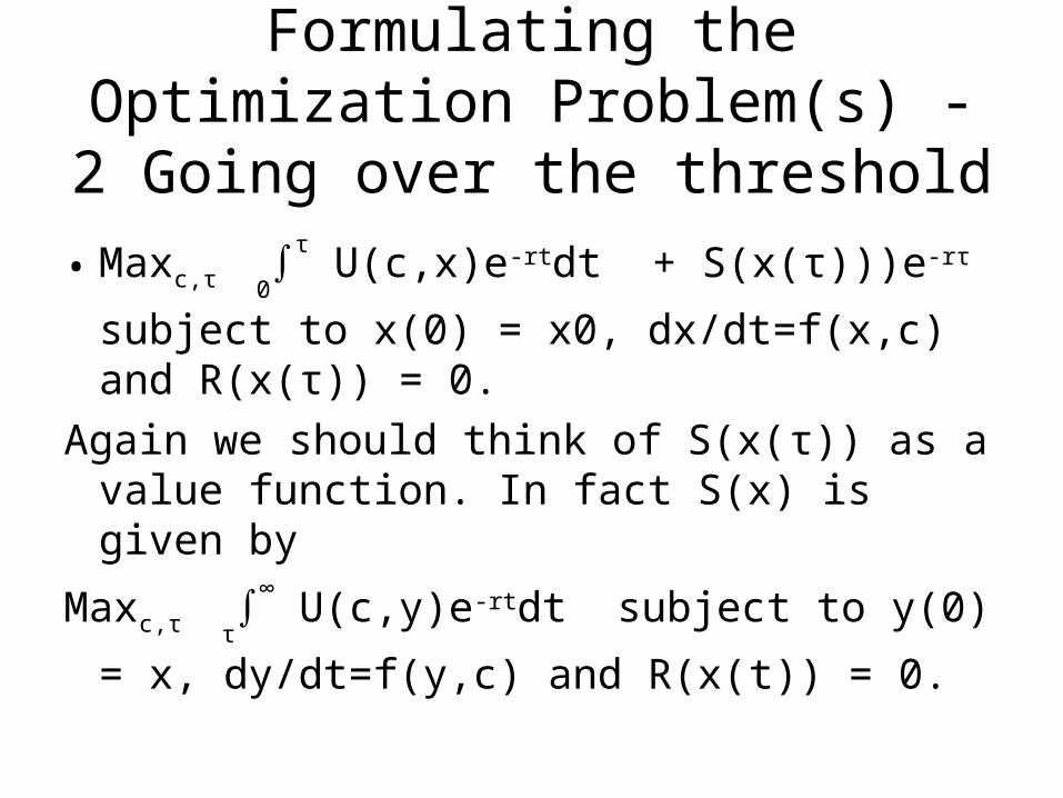
Formulating the Optimization Problem(s) - 2 Going over the
threshold
• Maxc,τ 0∫τ U(c,x)e-rtdt + S(x(τ)))e-rτ subject to
x(0) = x0, dx/dt=f(x,c) and R(x(τ)) = 0.
Again we should think of S(x(τ)) as a value function. In fact S(x) is given by
Maxc,τ τ∫∞ U(c,y)e-rtdt subject to y(0) = x,
dy/dt=f(y,c) and R(x(t)) = 0.

Solve the problem recursively
• From Maxc τ∫∞ U(c,y)e-rtdt subject to y(0) = x,
dy/dt=f(y,c), and R(x(t)) = 0. We get the shadow price λ*(x|τ).
• Note: Here I have excluded the possibility that R(x(t)) ≠ 0 for some t > τ. It is however perfectly possible that we may “turn away” from the threshold at some point in time. In particular if we are studying a finite horizon problem

Optimality conditions (Present value)
• u maximizes the Hamiltonian
• dλ/dt = –∂H/∂x
• λ(τ) = λ*(x(τ)|τ) + γ∂R/∂x
Note that all these may be vectors
• If τ lies in (0, ∞), then
• H + ∂(S(x(τ))) e-rτ)/∂t = 0
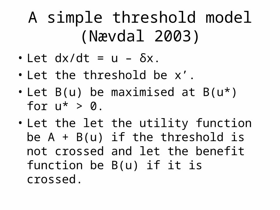
A simple threshold model (Nævdal 2003)
• Let dx/dt = u – δx.
• Let the threshold be x’.
• Let B(u) be maximised at B(u*) for u* > 0.
• Let the let the utility function be A + B(u) if the threshold is not crossed and let the benefit function be B(u) if it is crossed.
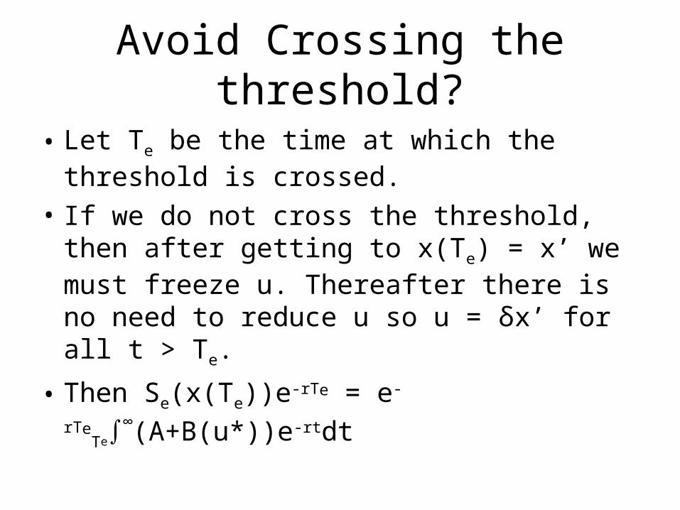
Avoid Crossing the threshold?
• Let Te be the time at which the threshold is crossed.
• If we do not cross the threshold, then after getting to x(Te) = x’ we must freeze u. Thereafter there is no need to reduce u so u = δx’ for all t > Te.
• Then Se(x(Te))e-rTe = e-rTeTe∫
∞(A+B(u*))e-rtdt

Crossing the threshold?
• Let Ta be the time at which the threshold is crossed.
• If we cross the threshold, then we accept the damage. Thereafter there is no need to reduce u so u = u* for all t > Ta.
• Then Sa(x(Ta))e-rTa = e-rTaTa∫
∞B(u*)e-rtdt
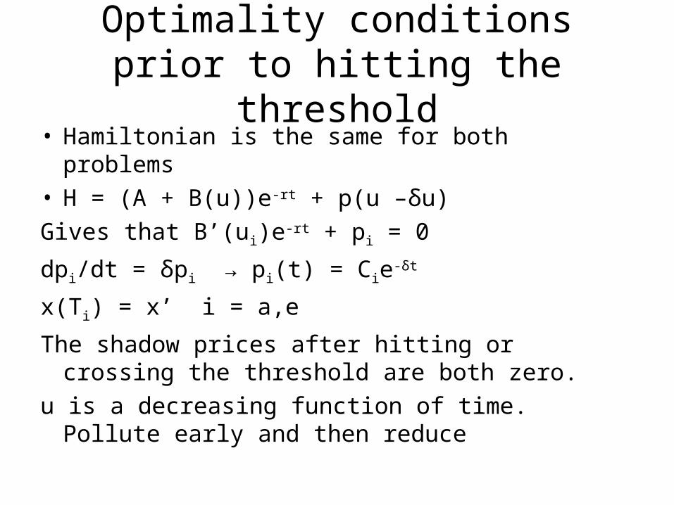
Optimality conditions prior to hitting the threshold
• Hamiltonian is the same for both problems• H = (A + B(u))e-rt + p(u –δu)
Gives that B’(ui)e-rt + pi = 0
dpi/dt = δpi → pi(t) = Cie-δt
x(Ti) = x’ i = a,e
The shadow prices after hitting or crossing the threshold are both zero.
u is a decreasing function of time. Pollute early and then reduce
Note
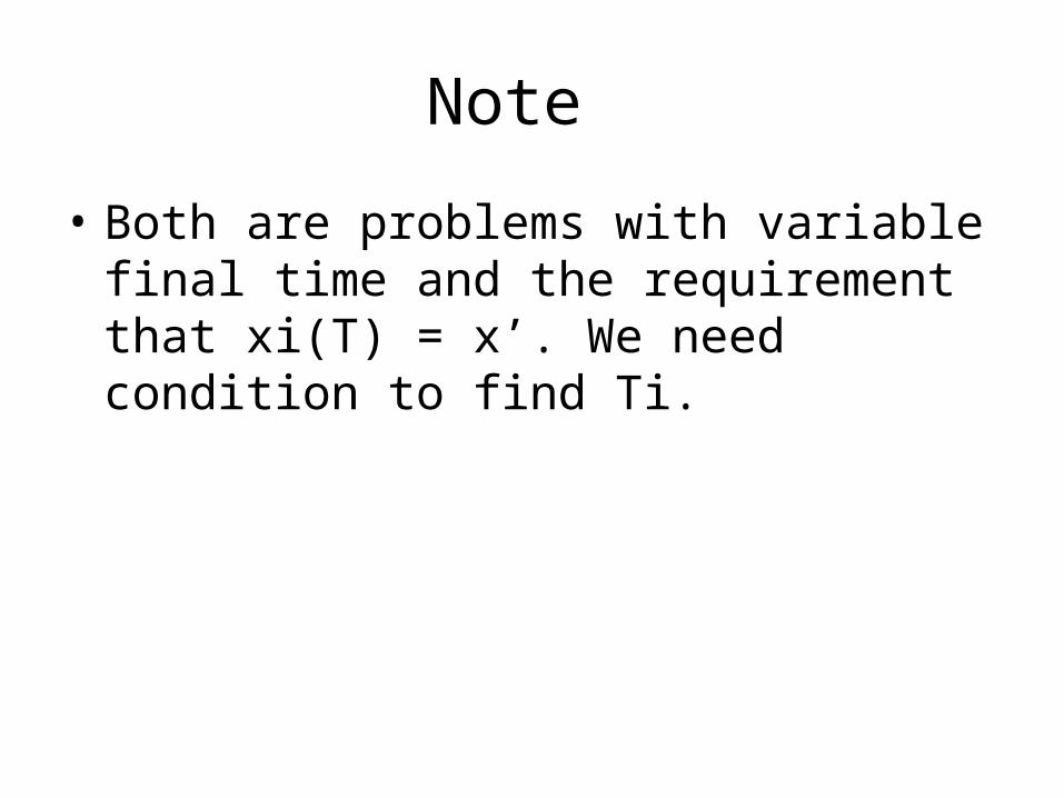
• Both are problems with variable final time and the requirement that xi(T) = x’. We need condition to find Ti.
Going over the threshold
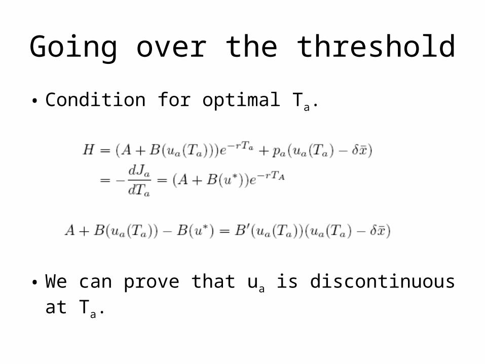
• Condition for optimal Ta.
• We can prove that ua is discontinuous at Ta.

Optimal paths of ua and xa
Staying on the edge
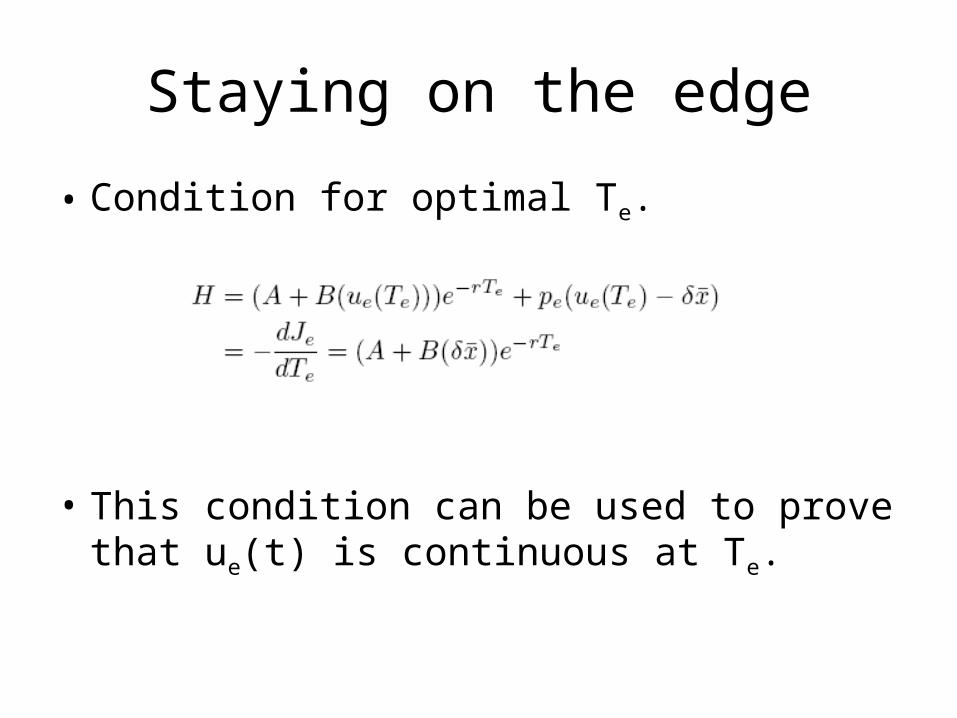
• Condition for optimal Te.
• This condition can be used to prove that ue(t) is continuous at Te.

Optimal paths of ue and xe

Important to note
• There are kinks (ue) or jumps (ua) in the optimal paths of the control.
• The previous literature on deterministic thresholds had overlooked:
1. That a threshold could either be crossed or observed
2. That optimal controls may be discontinuous at the time the threshold is crossed. (In some models this can happen when the threshold is reached even if it is not crossed.)

Comparing Scenarios
I said no proofs, but this one is rather instructive and a good example of how simple proofs can give interesting results
Incorporating uncertainty into optimal control
• Most processes are subject to uncertainty
• One class is Brownian motion. I will not talk about that at all.
• Catastrophic events.– Tsunamis– Floods– Car breakdown
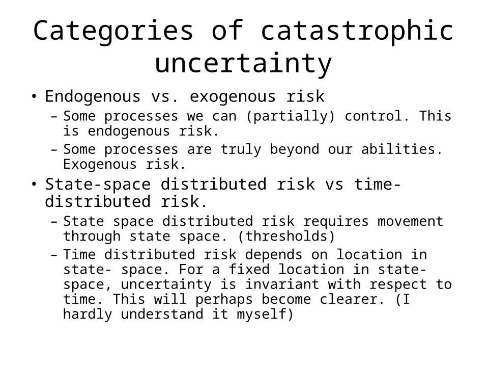
Categories of catastrophic uncertainty
• Endogenous vs. exogenous risk– Some processes we can (partially) control. This is
endogenous risk.– Some processes are truly beyond our abilities. Exogenous
risk.
• State-space distributed risk vs time-distributed risk.– State space distributed risk requires movement through
state space. (thresholds)– Time distributed risk depends on location in state- space.
For a fixed location in state-space, uncertainty is invariant with respect to time. This will perhaps become clearer. (I hardly understand it myself)
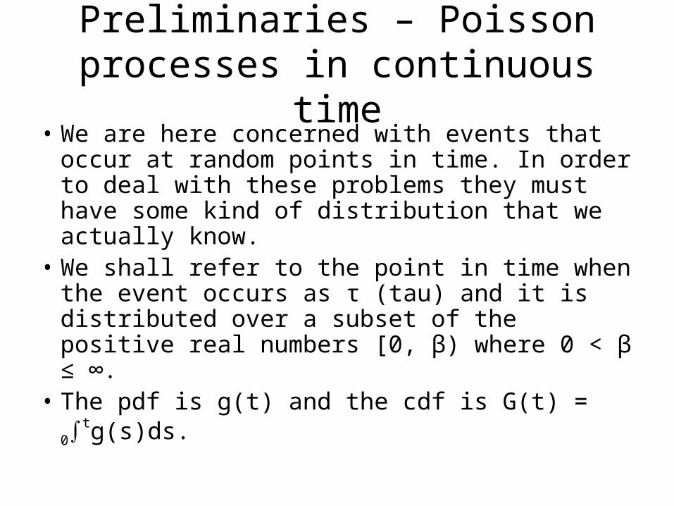
Preliminaries – Poisson processes in continuous time
• We are here concerned with events that occur at random points in time. In order to deal with these problems they must have some kind of distribution that we actually know.
• We shall refer to the point in time when the event occurs as τ (tau) and it is distributed over a subset of the positive real numbers [0, β) where 0 < β ≤ ∞.
• The pdf is g(t) and the cdf is G(t) = 0∫tg(s)ds.

Poisson processes and conditional updating.
• Our process starts t = 0. We make it to t* >0. What is the distribution of τ conditional on us having made it to t*?
Answer:
We need optimality conditions that reflect updating of the distribution as long as τ does not happen.
*
*|
tdssg
tgtttg

The hazard rate - A very useful concept
• We ask the question; What if we have made it to time t? What is the probability that τ occurs in the time interval (t, t + Δt)?
• If dt is small, then that probability is roughly Pr(τ (t, t + Δt))=g(t|τ>t)×dt.
• g(t|τ>1) is of course:
tdssg
tgtttg 1|
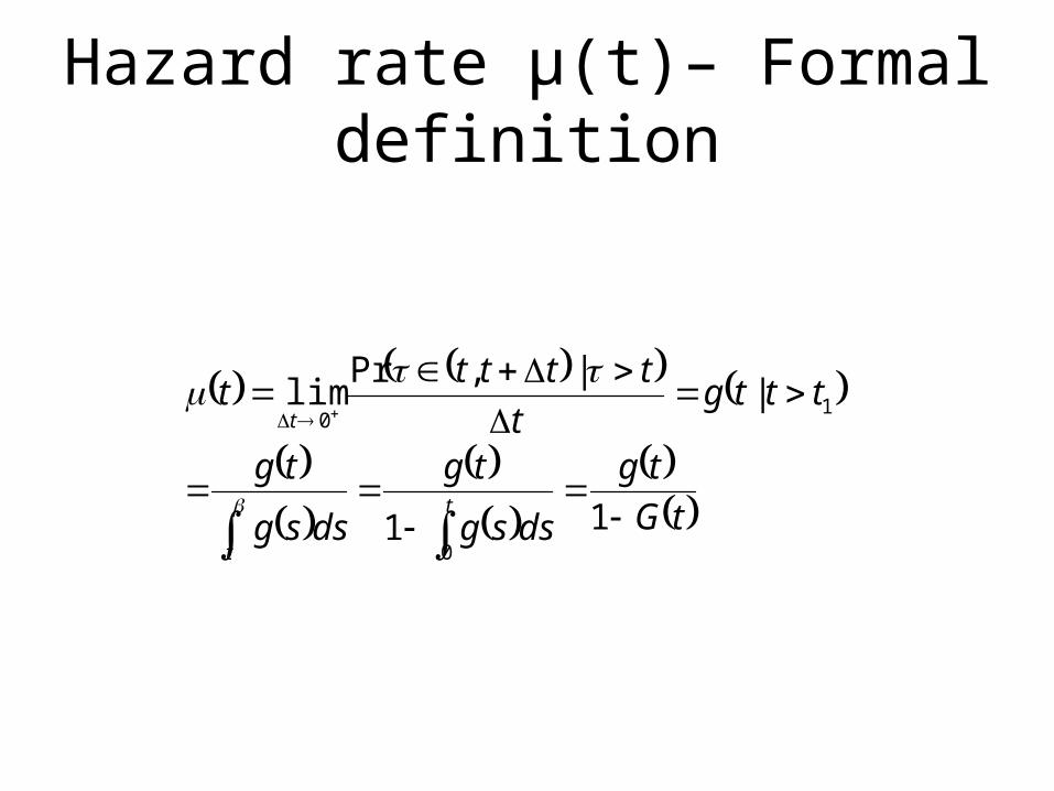
Hazard rate μ(t)– Formal definition
tG
tg
dssg
tg
dssg
tg
tttgt
ttttt
t
t
t
11
||,Pr
lim
0
10
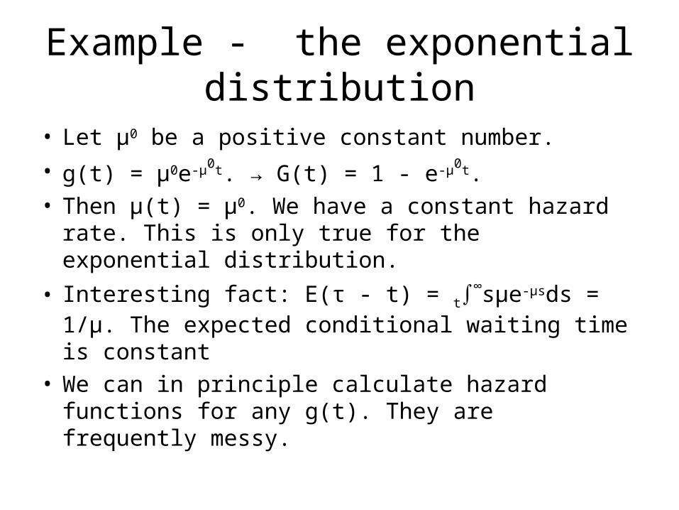
Example - the exponential distribution
• Let μ0 be a positive constant number.
• g(t) = μ0e-μ0t. → G(t) = 1 - e-μ0t.• Then μ(t) = μ0. We have a constant hazard rate. This
is only true for the exponential distribution.
• Interesting fact: E(τ - t) = t∫∞sµe-µsds = 1/µ. The
expected conditional waiting time is constant• We can in principle calculate hazard functions for any
g(t). They are frequently messy.
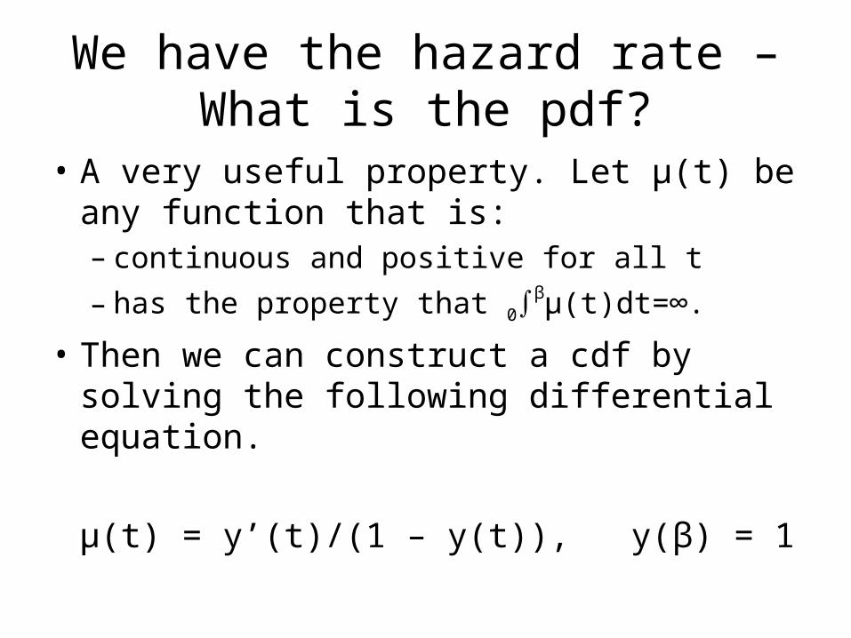
We have the hazard rate – What is the pdf?
• A very useful property. Let μ(t) be any function that is:– continuous and positive for all t
– has the property that 0∫βμ(t)dt=∞.
• Then we can construct a cdf by solving the following differential equation.
μ(t) = y’(t)/(1 – y(t)), y(β) = 1
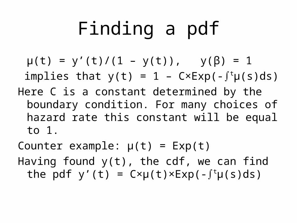
Finding a pdf
μ(t) = y’(t)/(1 – y(t)), y(β) = 1
implies that y(t) = 1 – C×Exp(-∫tμ(s)ds)
Here C is a constant determined by the boundary condition. For many choices of hazard rate this constant will be equal to 1.
Counter example: μ(t) = Exp(t)
Having found y(t), the cdf, we can find the pdf y’(t) = C×μ(t)×Exp(-∫tμ(s)ds)

Example – linear hazard rate
• Assume that μ(t) = μ0t defined for t € [0, ∞). Then Exp(-∫tμ(s)ds) = ½μ0t2. Therefore
y(t) = 1 – C× Exp(-½μ0t2) . y(∞) = 1 implies that C = 1, so the cdf is 1 – Exp(-½μ0t2) and the pdf is y’(t) = μ0t×Exp(-½μ0t2) .
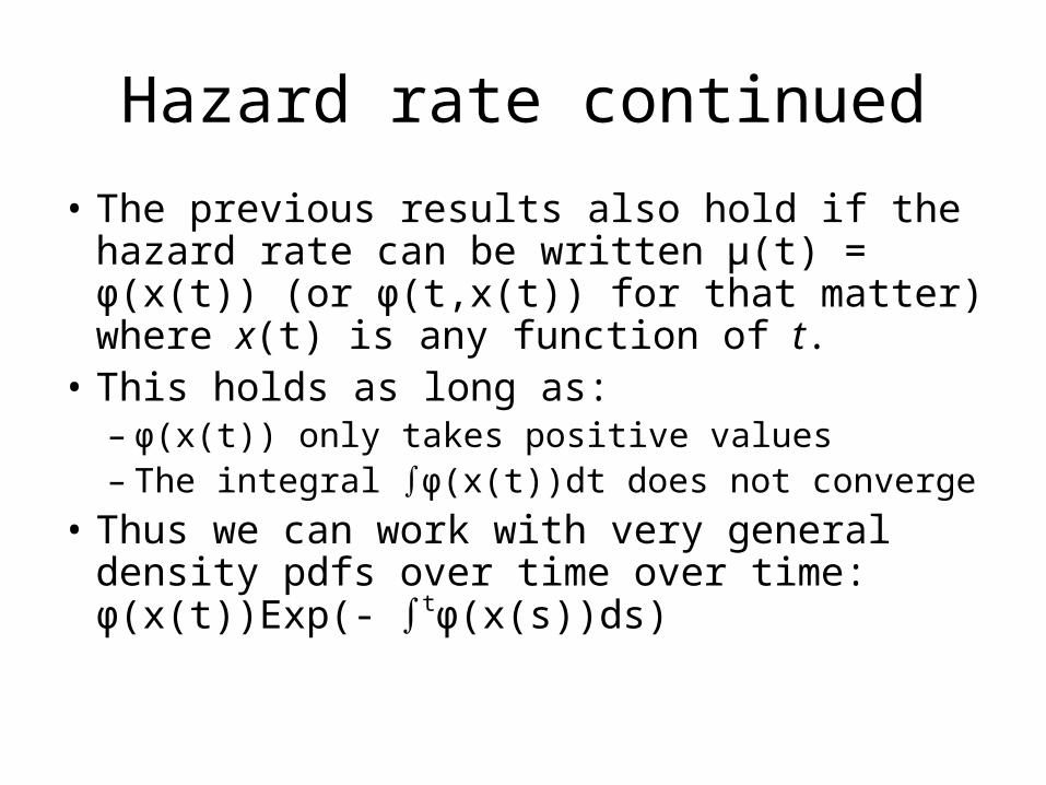
Hazard rate continued
• The previous results also hold if the hazard rate can be written μ(t) = φ(x(t)) (or φ(t,x(t)) for that matter) where x(t) is any function of t.
• This holds as long as:– φ(x(t)) only takes positive values– The integral ∫φ(x(t))dt does not converge
• Thus we can work with very general density pdfs over time over time: φ(x(t))Exp(- ∫tφ(x(s))ds)

Exogenous vs endogenous uncertainty
• Slightly confusing literature. Here the difference is as follows.
• If φ(x(t))is the hazard rate and x(t) is determined by a controllable differential equation, then the stochastic process is endogenous.
• If not, the process is exogenous• his is not clear cut. Hurricanes may be (in part)
endogenous to US policymakers but exogenous New Orleans

Controlling exogenous catastrophic uncertainty
• Basic problem: Nature or (somebody we can’t affect) triggers a catastrophic event.
• We can not control the probability of the event occurring, but we can control:– preparedness (what to do before the event)– consequences (how to act after the event)
• No strict boundary between preparedness and consequence management.
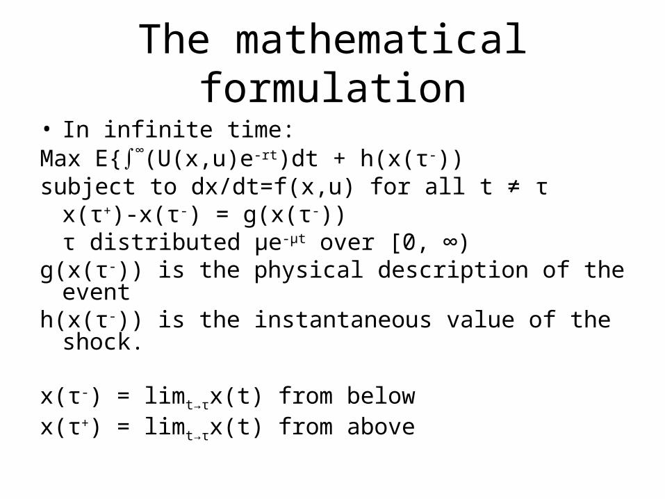
The mathematical formulation
• In infinite time:Max E{∫∞(U(x,u)e-rt)dt + h(x(τ-))subject to dx/dt=f(x,u) for all t ≠ τ
x(τ+)-x(τ-) = g(x(τ-))τ distributed μe-μt over [0, ∞)
g(x(τ-)) is the physical description of the eventh(x(τ-)) is the instantaneous value of the shock.
x(τ-) = limt→τx(t) from belowx(τ+) = limt→τx(t) from above
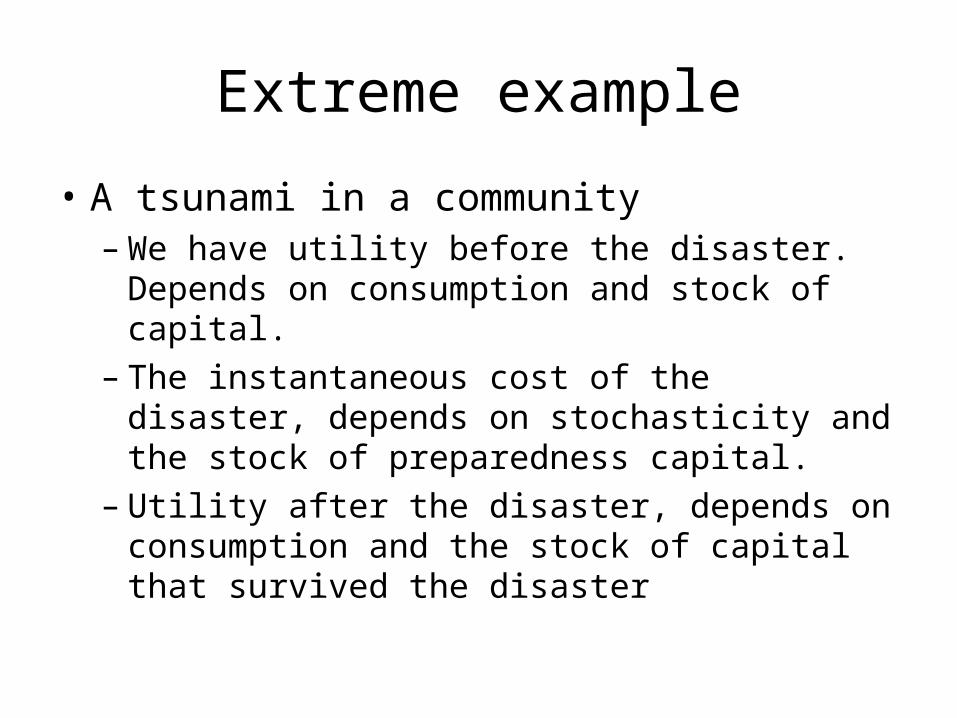
Extreme example
• A tsunami in a community– We have utility before the disaster. Depends on
consumption and stock of capital. – The instantaneous cost of the disaster, depends on
stochasticity and the stock of preparedness capital.– Utility after the disaster, depends on consumption
and the stock of capital that survived the disaster
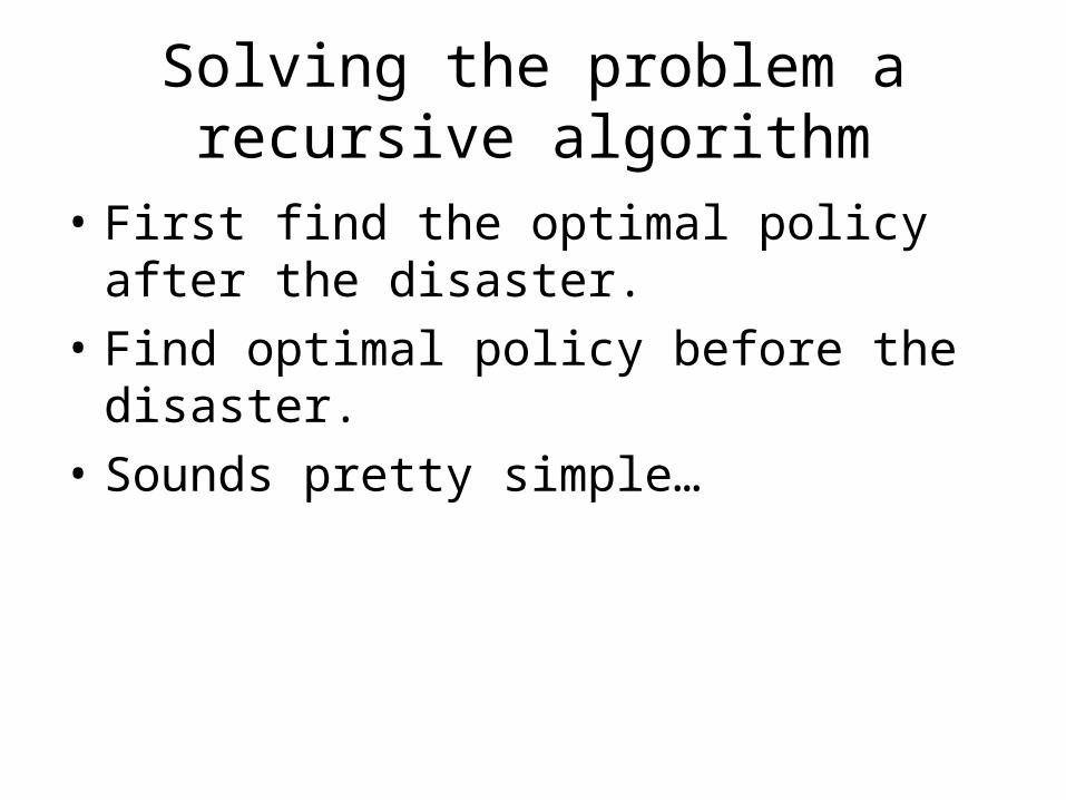
Solving the problem a recursive algorithm
• First find the optimal policy after the disaster.
• Find optimal policy before the disaster.
• Sounds pretty simple…
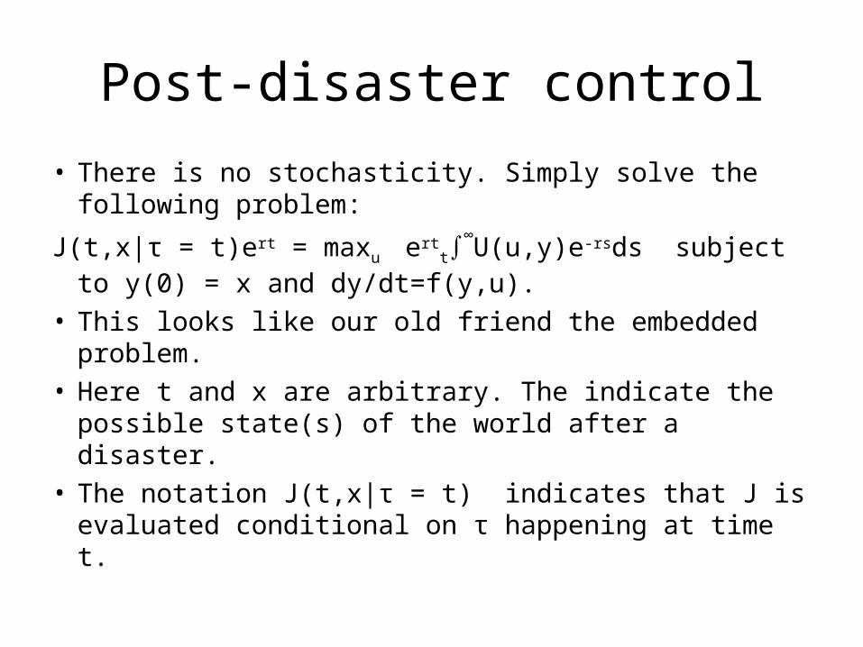
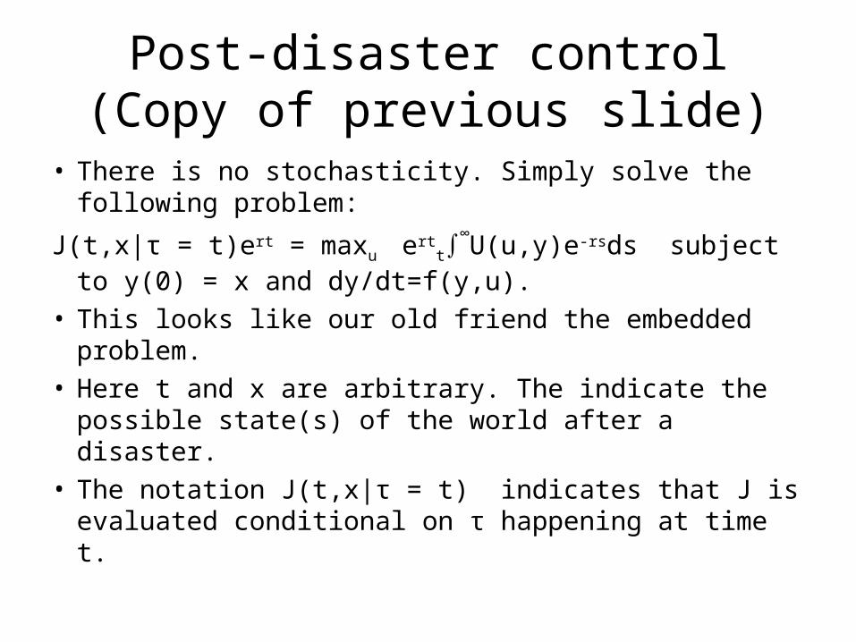
Post-disaster control
• There is no stochasticity. Simply solve the following problem:
J(t,x|τ = t)ert = maxu ertt∫
∞U(u,y)e-rsds subject to y(0) = x
and dy/dt=f(y,u). • This looks like our old friend the embedded problem. • Here t and x are arbitrary. The indicate the possible
state(s) of the world after a disaster.• The notation J(t,x|τ = t) indicates that J is evaluated
conditional on τ happening at time t.
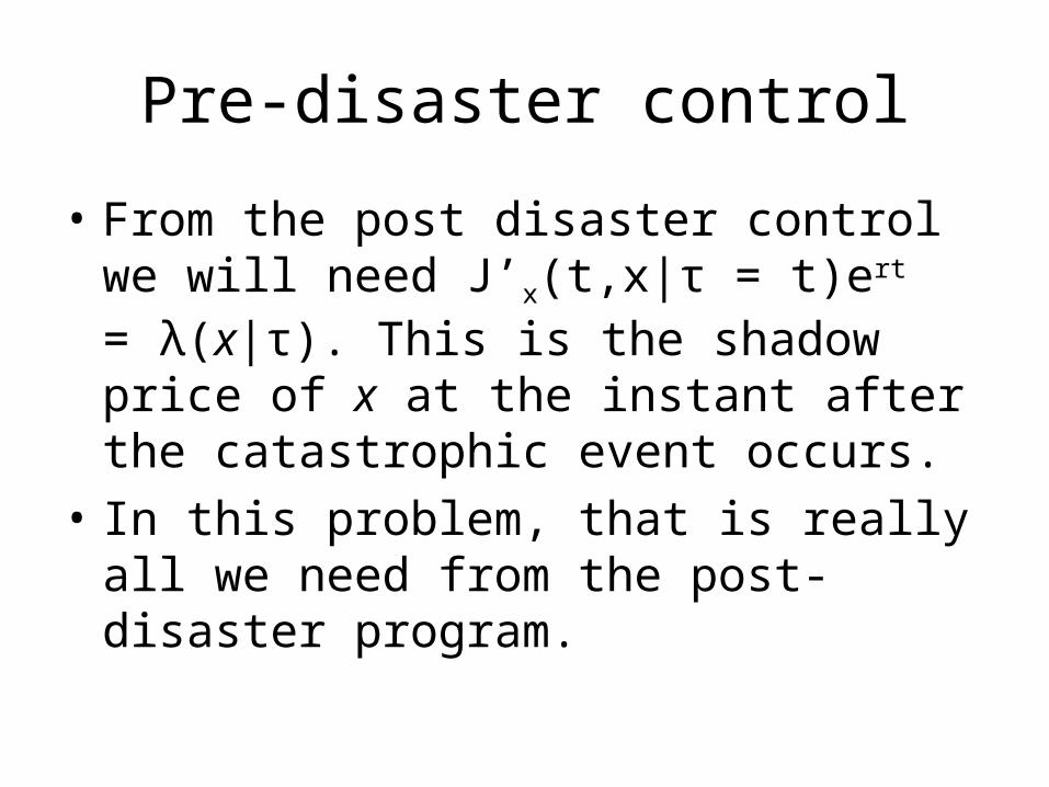
Pre-disaster control
• From the post disaster control we will need J’x(t,x|τ = t)ert = λ(x|τ). This is the shadow price of x at the instant after the catastrophic event occurs.
• In this problem, that is really all we need from the post-disaster program.

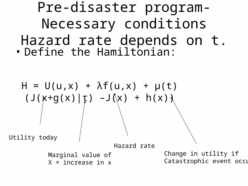
Pre-disaster program- Necessary conditions Hazard rate depends on t.
• Define the Hamiltonian:
H = U(u,x) + λf(u,x) + µ(t)(J(x+g(x)|τ) –J(x) + h(x))
Utility today
Marginal value ofX × increase in x
Hazard rateChange in utility if Catastrophic event occurs

Optimality Conditions
• Apply the maximum principle to the Hamiltonian.
• u =argmax H
• dλ/dt = rλ - ∂H/∂x
• dx/dt=f(x,u)
• Transversality condition as in deterministic models.
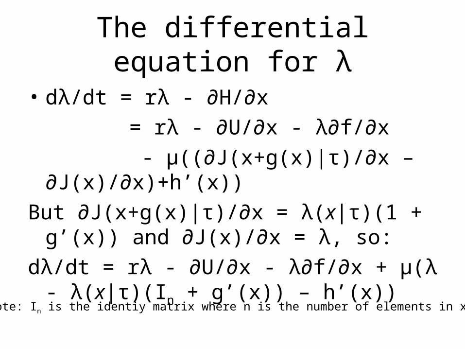
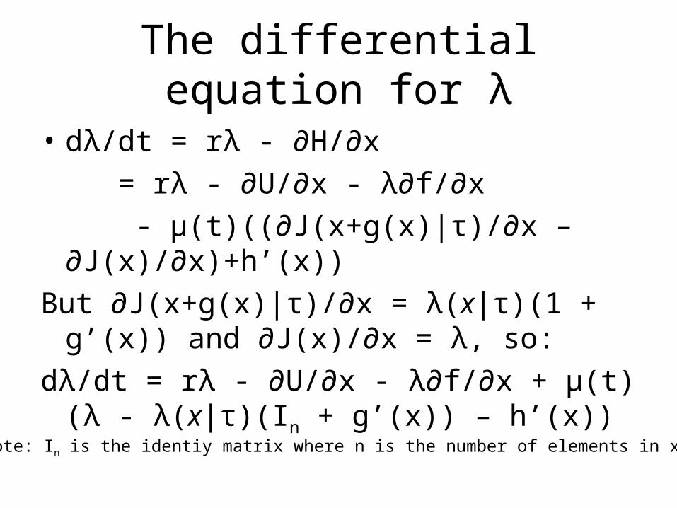
The differential equation for λ
• dλ/dt = rλ - ∂H/∂x
= rλ - ∂U/∂x - λ∂f/∂x
- µ((∂J(x+g(x)|τ)/∂x –∂J(x)/∂x)+h’(x))
But ∂J(x+g(x)|τ)/∂x = λ(x|τ)(1 + g’(x)) and ∂J(x)/∂x = λ, so:
dλ/dt = rλ - ∂U/∂x - λ∂f/∂x + µ(λ - λ(x|τ)(In + g’(x)) – h’(x))
Note: In is the identiy matrix where n is the number of elements in x(t)
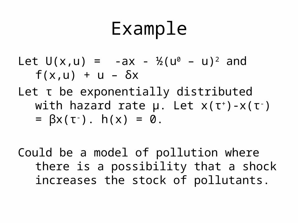
Example
Let U(x,u) = -ax - ½(u0 – u)2 and f(x,u) + u – δx
Let τ be exponentially distributed with hazard rate µ. Let x(τ+)-x(τ-) = βx(τ-). h(x) = 0.
Could be a model of pollution where there is a possibility that a shock increases the stock of pollutants.

Optimality conditions after event
H= -ax - ½(u0 – u)2 + λ(u – δx)1. The value of u that maximizes the
Hamiltonian is given by u = u0 + λ for u0 + λ > 0. Else u = 0.
2. dλ/dt = rλ + a + δλ 3. dx/dt = u0 + λ – δxdλ/dt = rλ + a + δλ → λ(t|τ) = -a/(r + δ) for all t.
We make note of λ(t|τ) and proceed to the pre-event control

Pre event conditions
1. The value of u that maximizes the Hamiltonian is given by u = u0 + ½λ for u0 + ½λ > 0. Else u = 0. Same as before!
2. dx/dt = u0 + ½λ – δx. Same as before!
3. dλ/dt = rλ + a + δλ +µ(λ – (–a(1+β)/(r + δ)))
Here is the difference in the conditions. Obviously this implies that u and x will be affectedby the risk
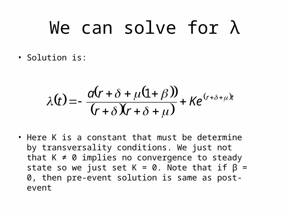
We can solve for λ
• Solution is:
• Here K is a constant that must be determine by transversality conditions. We just not that K ≠ 0 implies no convergence to steady state so we just set K = 0. Note that if β = 0, then pre-event solution is same as post-event
trKerr
rat
l
1

The we have that….
• The optimal value of u(t) is found by inserting λ(t) into u0 + ½λ.
• The optimal value of x(t) is fund by integrating dx/dt = u0 + ½λ – δx
• I will not do this as the resulting expression is a bugger.
• Numeric solutions are straightforward to find

Entering Equations in Excel
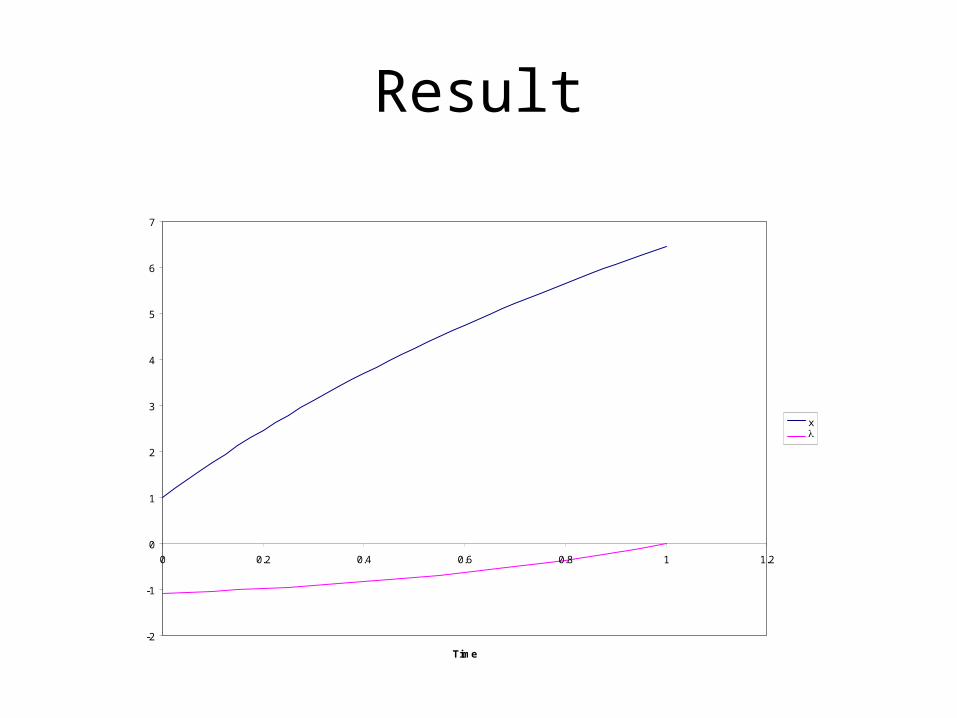
Result
-2
-1
0
1
2
3
4
5
6
7
0 0.2 0.4 0.6 0.8 1 1.2
Time
xl

The effect of uncertainty – Let us increase µ
-6
-4
-2
0
2
4
6
8
10
0 0.5 1 1.5 2 2.5 3 3.5
Time
0.5l 0.5 1l 1 2l 2

Weird hazard rates
• The setup is good enough to include time dependent hazard rates. That is, the hazard rate depends on time.
• Let us consider a hazard rate a×(Sin(t) + 1). This implies a cdf given by 1 – exp(-1-t+Cos(t)). Cdf looks like this:
2 4 6 8
0.965
0.97
0.975
0.98
0.985
0.99
0.995
Pre-disaster program- Necessary conditions Hazard rate depends on t.
• Define the Hamiltonian:
H = U(u,x) + λf(u,x) + µ(t)(J(x+g(x)|τ) –J(x) + h(x))
Utility today
Marginal value ofX × increase in x
Hazard rateChange in utility if Catastrophic event occurs

Optimality Conditions
• Apply the maximum principle to the Hamiltonian.
• u =argmax H
• dλ/dt = rλ - ∂H/∂x
• dx/dt=f(x,u)
• Transversality condition as in deterministic models.
NO CHANGE!
The differential equation for λ
• dλ/dt = rλ - ∂H/∂x
= rλ - ∂U/∂x - λ∂f/∂x
- µ(t)((∂J(x+g(x)|τ)/∂x –∂J(x)/∂x)+h’(x))
But ∂J(x+g(x)|τ)/∂x = λ(x|τ)(1 + g’(x)) and ∂J(x)/∂x = λ, so:
dλ/dt = rλ - ∂U/∂x - λ∂f/∂x + µ(t)(λ - λ(x|τ)(In + g’(x)) – h’(x))
Note: In is the identiy matrix where n is the number of elements in x(t)
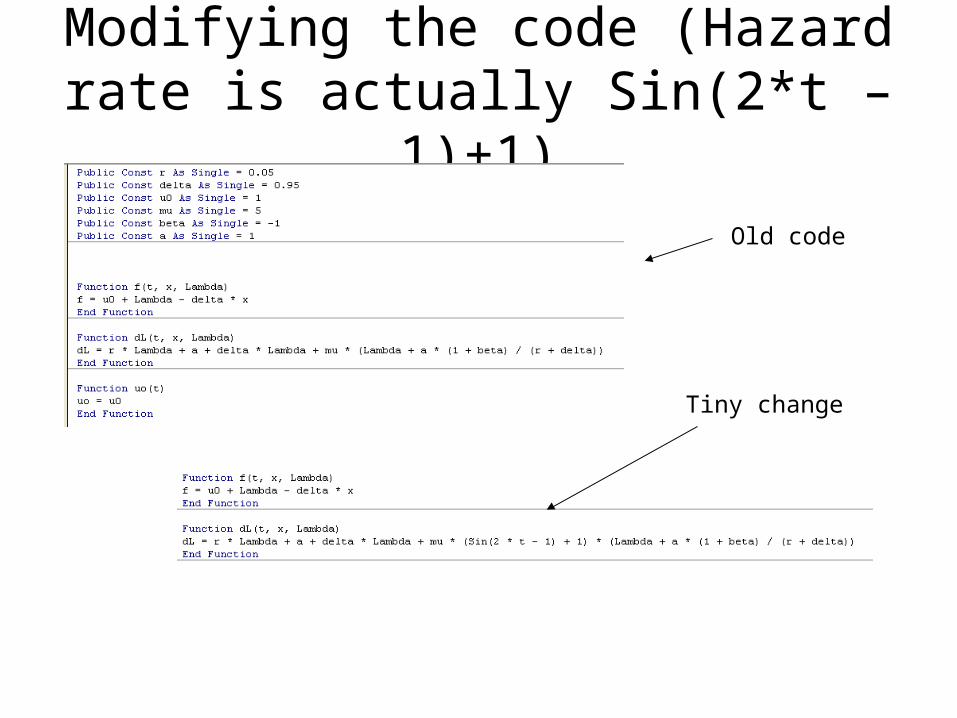
Modifying the code (Hazard rate is actually Sin(2*t – 1)+1)
Old code
Tiny change
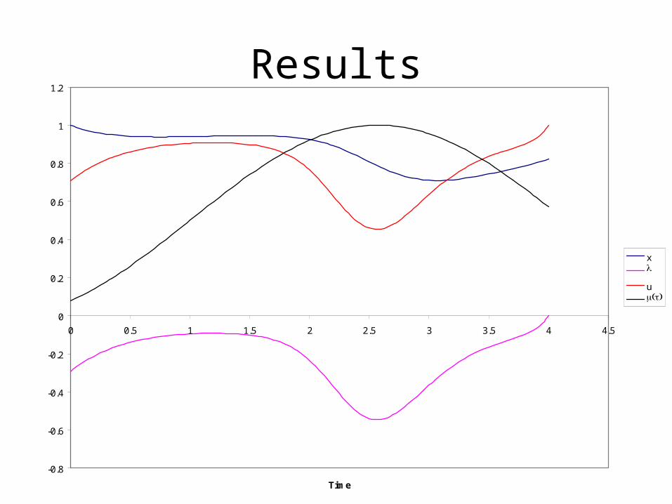
Results
-0.8
-0.6
-0.4
-0.2
0
0.2
0.4
0.6
0.8
1
1.2
0 0.5 1 1.5 2 2.5 3 3.5 4 4.5
Time
xl
u

Endogenous risk – Time distributed
• Recall that we know face a controllable hazard rate.
• The hazard rate depends on a state variable
Endogenous time distributed risk
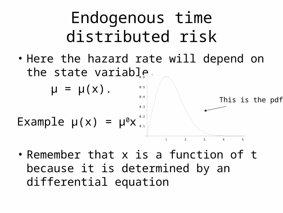
• Here the hazard rate will depend on the state variable.
µ = µ(x).
Example µ(x) = µ0x
• Remember that x is a function of t because it is determined by an differential equation
1 2 3 4 5
0.1
0.2
0.3
0.4
0.5
0.6
This is the pdf
Endogenous risk continued
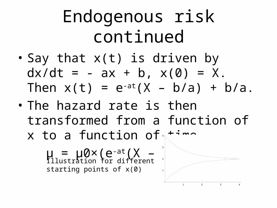
• Say that x(t) is driven by dx/dt = - ax + b, x(0) = X. Then x(t) = e-at(X – b/a) + b/a.
• The hazard rate is then transformed from a function of x to a function of time.
µ = µ0×(e-at(X – b/a) + b/a)
1 2 3 4
1
2
3
4
Illustration for different starting points of x(0)
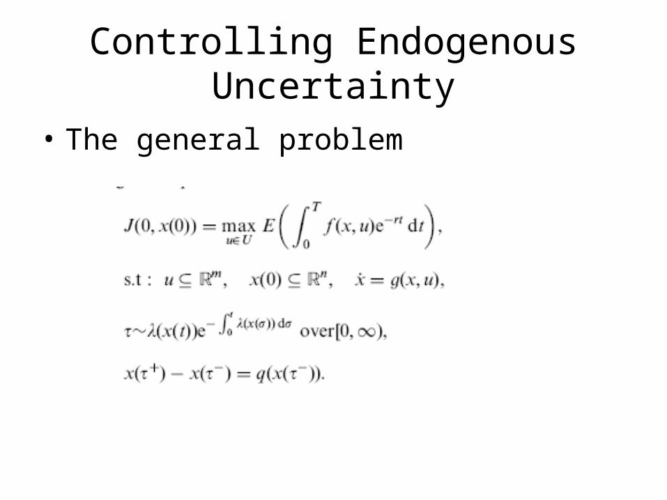
Controlling Endogenous Uncertainty
• The general problem
Recursivity - Working yourself backwards
• As before. First solve the post disaster problem. Get the shadow prices
Post-disaster control (Copy of previous slide)
• There is no stochasticity. Simply solve the following problem:
J(t,x|τ = t)ert = maxu ertt∫
∞U(u,y)e-rsds subject to y(0) = x
and dy/dt=f(y,u). • This looks like our old friend the embedded problem. • Here t and x are arbitrary. The indicate the possible
state(s) of the world after a disaster.• The notation J(t,x|τ = t) indicates that J is evaluated
conditional on τ happening at time t.
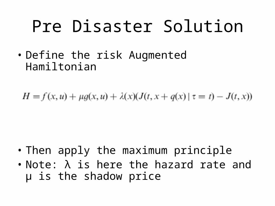
Pre Disaster Solution
• Define the risk Augmented Hamiltonian
• Then apply the maximum principle• Note: λ is here the hazard rate and µ is the
shadow price
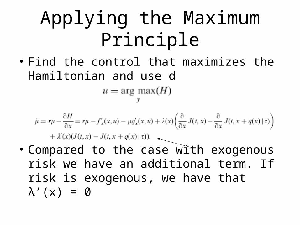
Applying the Maximum Principle
• Find the control that maximizes the Hamiltonian and use d
• Compared to the case with exogenous risk we have an additional term. If risk is exogenous, we have that λ’(x) = 0

A closer look at dµ/dt
• As in the exogenous risk case, we have that
• We have J(x+g(x)|τ) from the post-disaster problem. But what about J(x)?
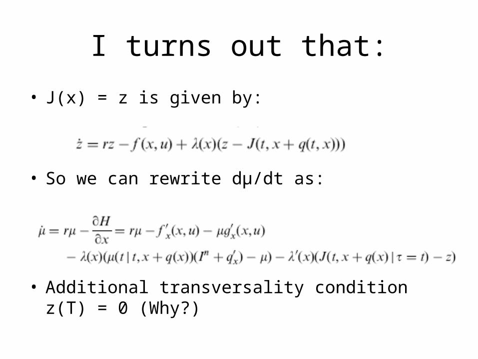
I turns out that:
• J(x) = z is given by:
• So we can rewrite dµ/dt as:
• Additional transversality condition z(T) = 0 (Why?)
A pedagogic problem
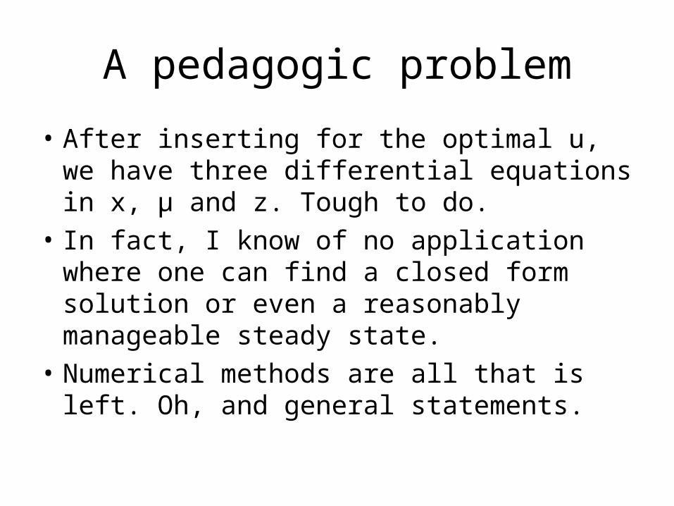
• After inserting for the optimal u, we have three differential equations in x, µ and z. Tough to do.
• In fact, I know of no application where one can find a closed form solution or even a reasonably manageable steady state.
• Numerical methods are all that is left. Oh, and general statements.

The Problem we are going to solve
,
. rate hazard with variablerandom
.00,0given, 0,..
2
1max
0
0
20
K
tx
xxuxts
dteuuET
rt

The post event solution
• Really simple. No more damage from x so post event shadow price is zero.
• This implies that u = u0 for all t > τ.
• J(x|t) = -K/r
The pre-event problem
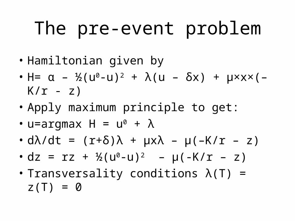
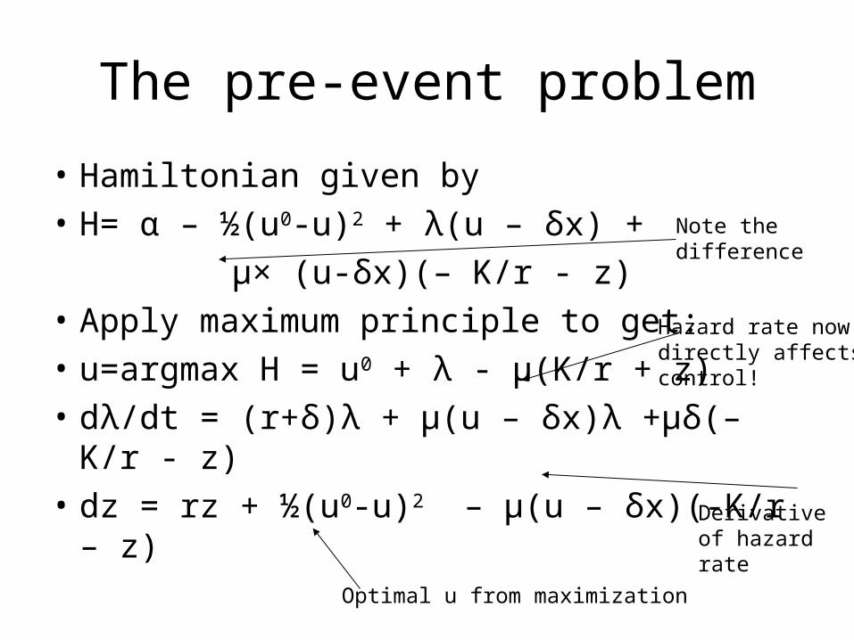
• Hamiltonian given by
• H= α – ½(u0-u)2 + λ(u – δx) + µ×x×(– K/r - z)
• Apply maximum principle to get:
• u=argmax H = u0 + λ
• dλ/dt = (r+δ)λ + µxλ – µ(–K/r – z)
• dz = rz + ½(u0-u)2 – µ(-K/r – z)
• Transversality conditions λ(T) = z(T) = 0
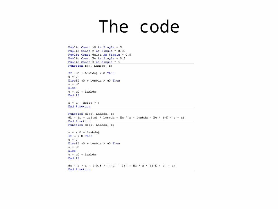
The code
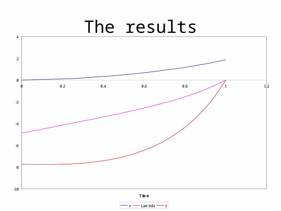
The results
-10
-8
-6
-4
-2
0
2
4
0 0.2 0.4 0.6 0.8 1 1.2
Time
x Lambda z

Play around to deal with instability
• Load Excel file

Endogenous, state-space distributed risk – AKA stochastic
threshold
• We move a state variable through time. If we move in the “right” direction we may trigger a threshold effect.
Possible thresholdlocations
t
x(t)
Risky time segment
Preliminary math.
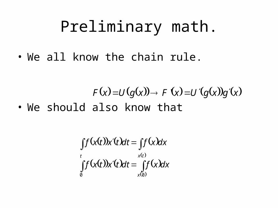
• We all know the chain rule.
• We should also know that xgxgUxFxgUxF '
tx
x
t
dxxfdttxtxf
dxxfdttxtxf
00
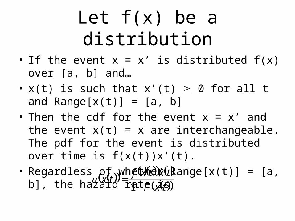
Let f(x) be a distribution
• If the event x = x’ is distributed f(x) over [a, b] and…• x(t) is such that x’(t) 0 for all t and Range[x(t)] =
[a, b]• Then the cdf for the event x = x’ and the event x(τ) =
x are interchangeable. The pdf for the event is distributed over time is f(x(t))x’(t).
• Regardless of whether Range[x(t)] = [a, b], the hazard rate is
txF
txtxftx
1

The hazard rate continued
• Note how the hazard rate depends on the rate of increase in x. dx/dt = 0 implies that the hazard rate is zero.
txF
txtxftx
1
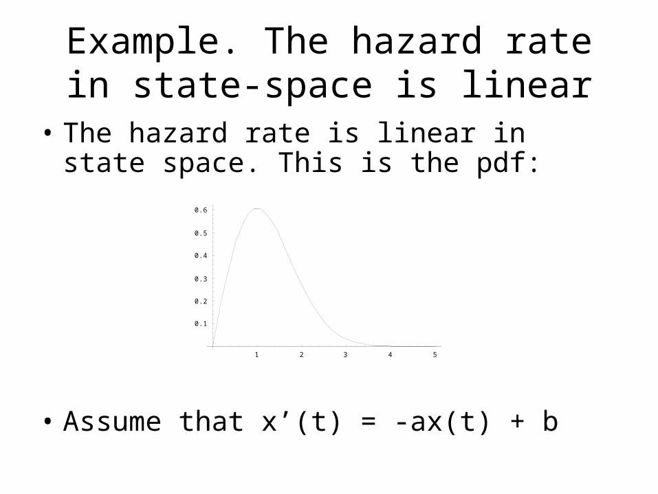
Example. The hazard rate in state-space is linear
• The hazard rate is linear in state space. This is the pdf:
• Assume that x’(t) = -ax(t) + b
1 2 3 4 5
0.1
0.2
0.3
0.4
0.5
0.6
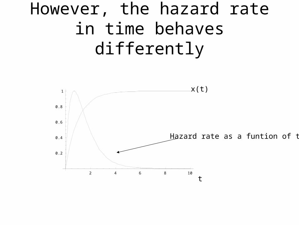
However, the hazard rate in time behaves differently
2 4 6 8 10
0.2
0.4
0.6
0.8
1 x(t)
Hazard rate as a funtion of time
t
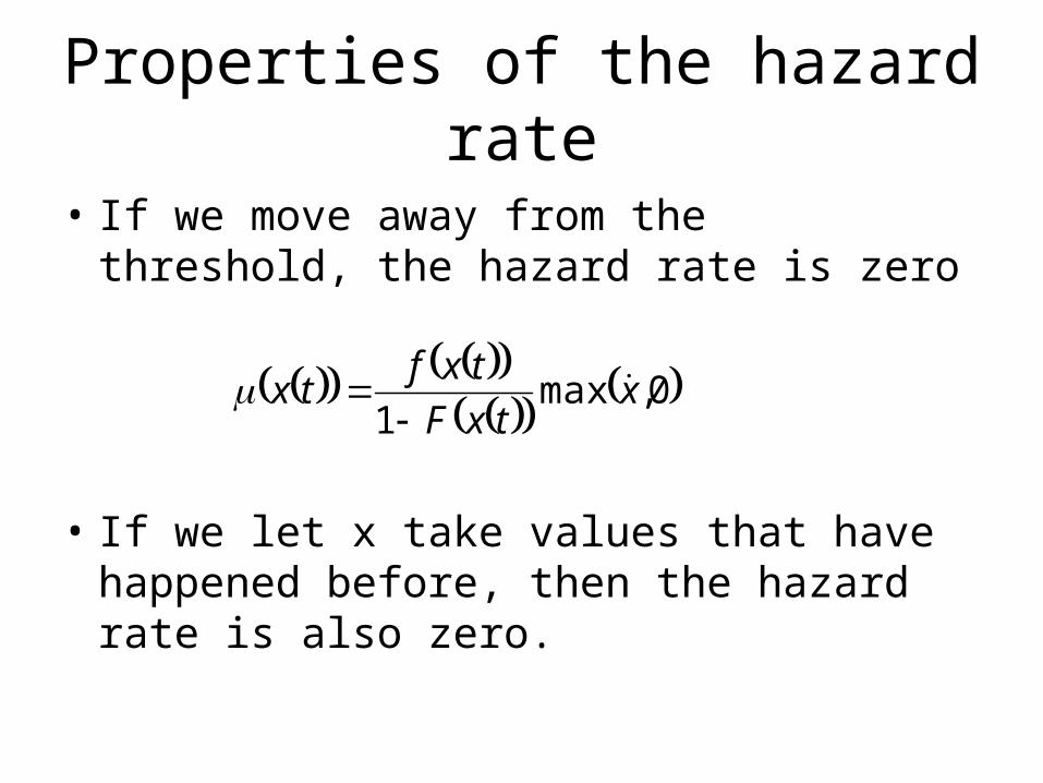
Properties of the hazard rate
• If we move away from the threshold, the hazard rate is zero
• If we let x take values that have happened before, then the hazard rate is also zero.
0,max
1x
txF
txftx
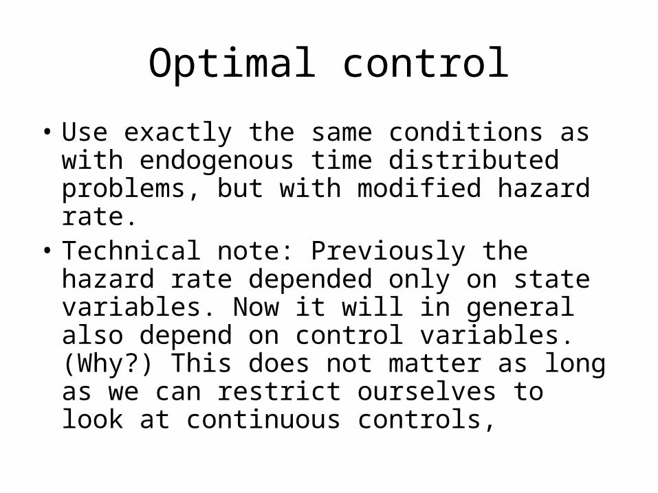
Optimal control
• Use exactly the same conditions as with endogenous time distributed problems, but with modified hazard rate.
• Technical note: Previously the hazard rate depended only on state variables. Now it will in general also depend on control variables. (Why?) This does not matter as long as we can restrict ourselves to look at continuous controls,

Example
• Same as before. However, this time we will consider a threshold problem.
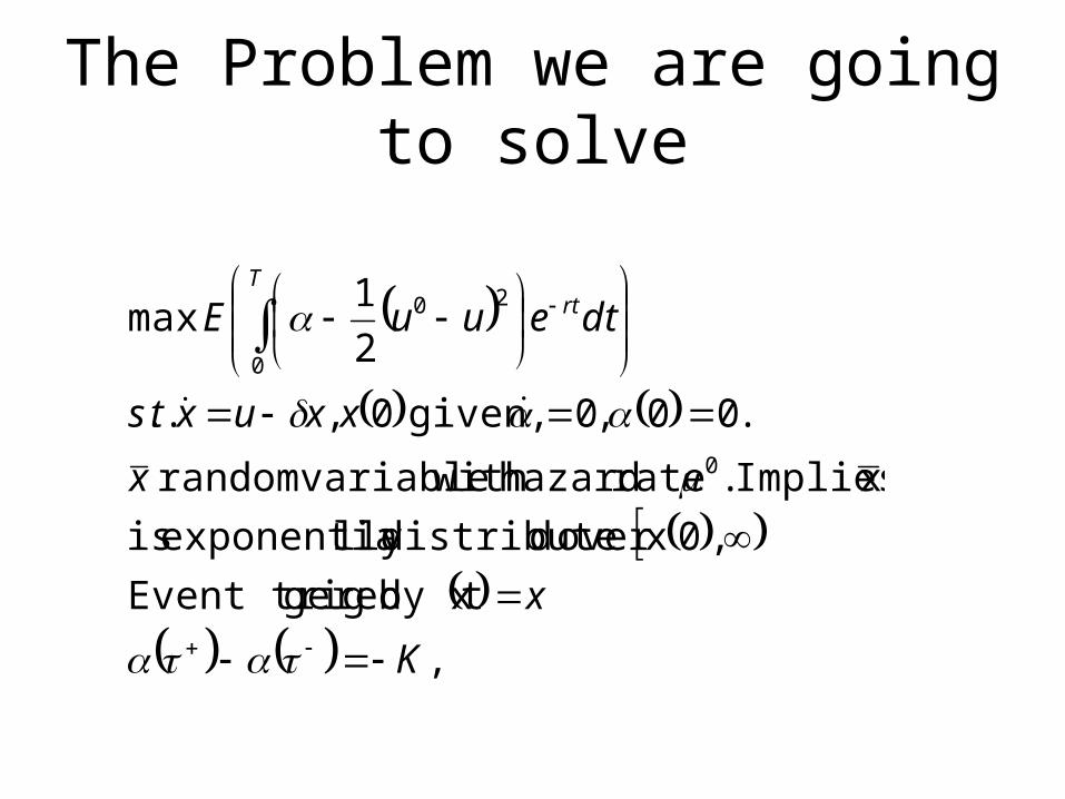
The Problem we are going to solve
,
tby x geredEvent trig
,0xover ddistributelly exponentia is
x Implies . rate hazard with variablerandom
.00,0given, 0,..
2
1max
0
0
20
K
x
x
xxuxts
dteuuET
rt
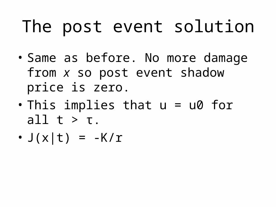
The post event solution
• Same as before. No more damage from x so post event shadow price is zero.
• This implies that u = u0 for all t > τ.
• J(x|t) = -K/r
The pre-event problem
• Hamiltonian given by
• H= α – ½(u0-u)2 + λ(u – δx) +
µ× (u-δx)(– K/r - z)
• Apply maximum principle to get:
• u=argmax H = u0 + λ - µ(K/r + z)
• dλ/dt = (r+δ)λ + µ(u – δx)λ +µδ(– K/r - z)
• dz = rz + ½(u0-u)2 – µ(u – δx)(-K/r – z)
Note the difference
Hazard rate nowdirectly affectscontrol!
Derivativeof hazard rate
Optimal u from maximization
Analytics
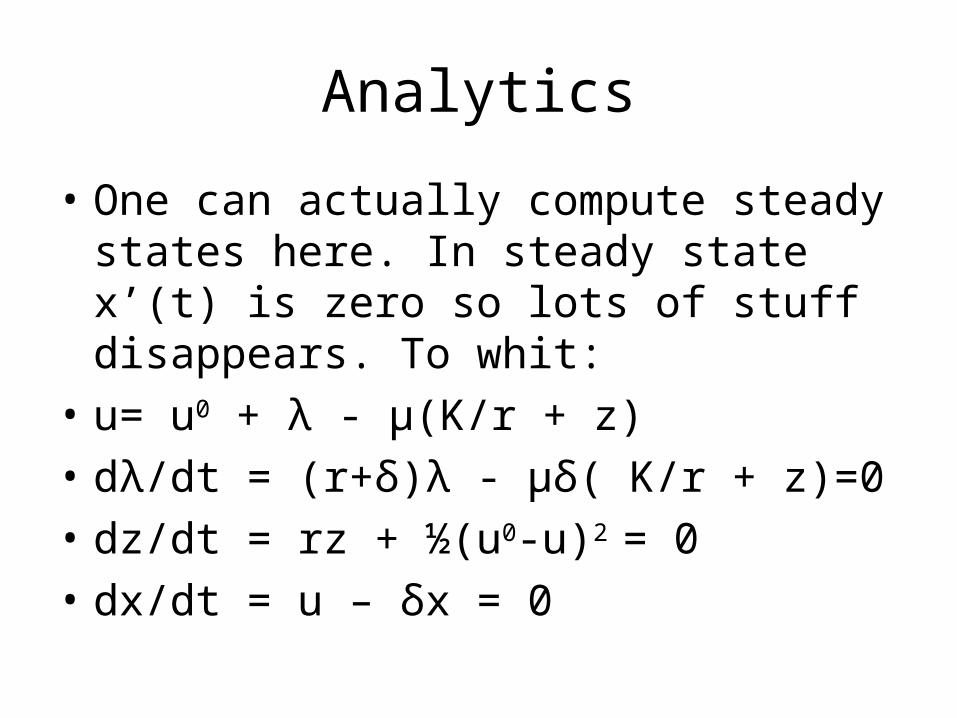
• One can actually compute steady states here. In steady state x’(t) is zero so lots of stuff disappears. To whit:
• u= u0 + λ - µ(K/r + z)
• dλ/dt = (r+δ)λ - µδ( K/r + z)=0
• dz/dt = rz + ½(u0-u)2 = 0
• dx/dt = u – δx = 0

Steady state solution
Krr
uu
Krrux
ss
ss
2
2
2
0
2
20
Note the following: K = 0 implies x and u equal to unregulated levelsOtherwise K > 0 implies small x and u. K large enough implies x and u less than zero in steady state.
A caveat
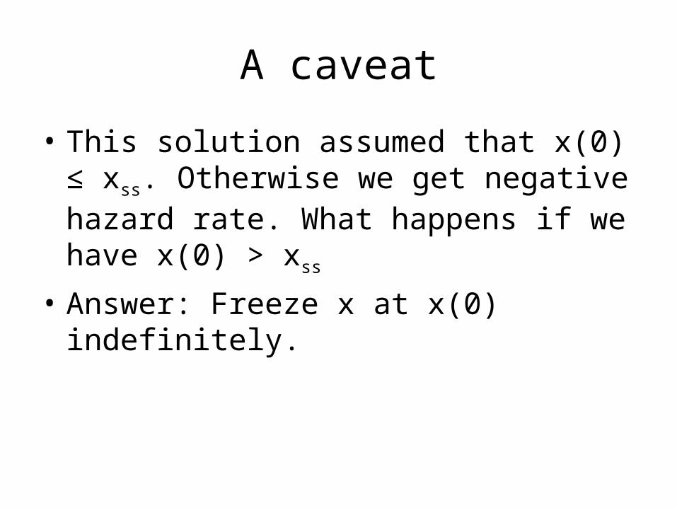
• This solution assumed that x(0) ≤ xss. Otherwise we get negative hazard rate. What happens if we have x(0) > xss
• Answer: Freeze x at x(0) indefinitely.
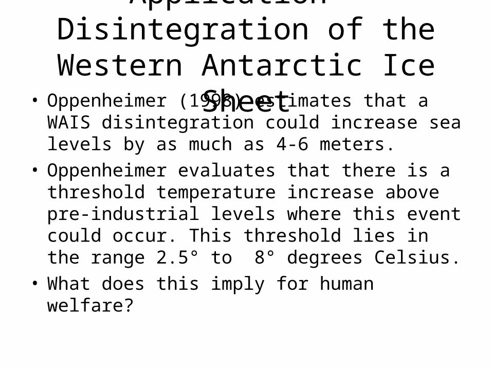
Application – Disintegration of the Western Antarctic Ice
Sheet• Oppenheimer (1998) estimates that a
WAIS disintegration could increase sea levels by as much as 4-6 meters.
• Oppenheimer evaluates that there is a threshold temperature increase above pre-industrial levels where this event could occur. This threshold lies in the range 2.5° to 8° degrees Celsius.
• What does this imply for human welfare?
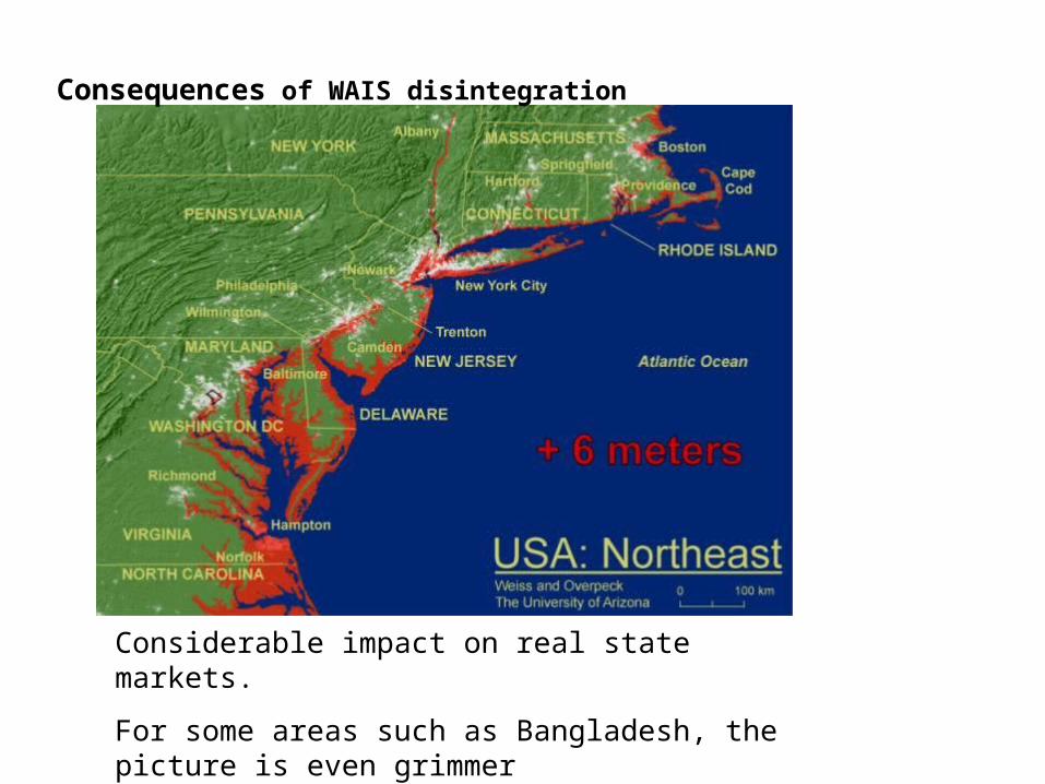
Consequences of WAIS disintegration
Considerable impact on real state markets.
For some areas such as Bangladesh, the picture is even grimmer
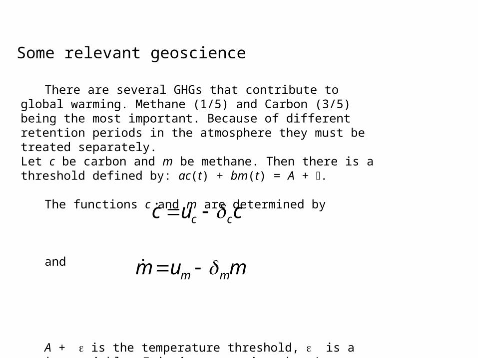
There are several GHGs that contribute to global warming. Methane (1/5) and Carbon (3/5) being the most important. Because of different retention periods in the atmosphere they must be treated separately.Let c be carbon and m be methane. Then there is a threshold defined by: ac(t) + bm(t) = A + .
The functions c and m are determined by
and
A + is the temperature threshold, is a random variable. Emissions are given by ui
Some relevant geoscience
mum mm
cuc cc
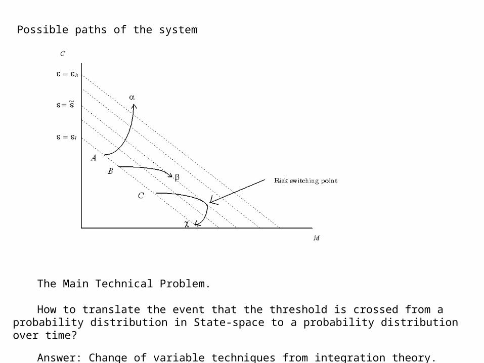
Possible paths of the system
The Main Technical Problem. How to translate the event that the threshold is crossed from a probability distribution in State-space to a probability distribution over time?
Answer: Change of variable techniques from integration theory.

We can now state society’s optimization problem as follows:
The Economy
The instantanous cost of emission reduction
The cost of crossing Wais disintegration: = G if threshold is crossed, = 0 otherwise
Steady states are calculated in the paper
miiuuK
uk iii
ii ,,2
20
0
2020, 22
max dtuuK
uuK
E mmm
ccc
uu mc
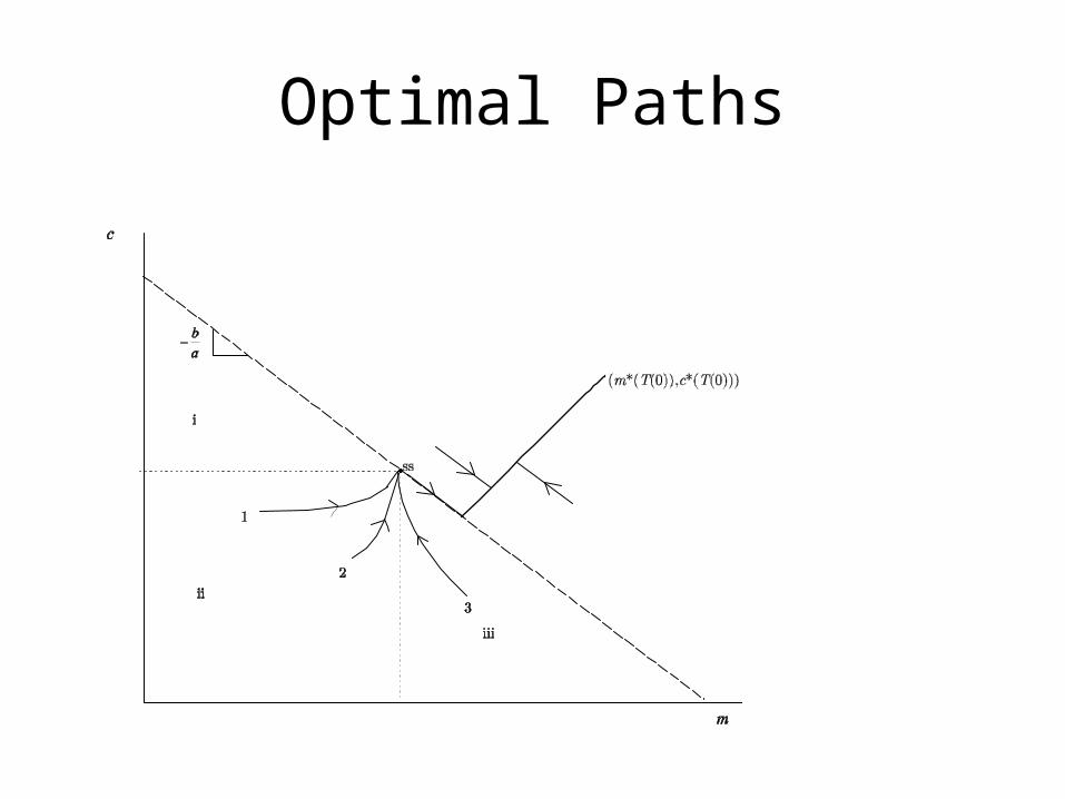
Optimal Paths
Optimal Stopping in Exogenous Risk Problems

Some numerical comparative dynamics
0.1 0.2 0.3 0.4 0.5 0.6 0.7 0.80.04
0.06
0.08
0.1
0.12
0.14
0.16
0.18
0.2
CO2
CH
4
Optimal path when c = 5.4
Steady state when c = 5.4
Optimal path when c = 5
Steady state when c = 5
Optimal path when c = 4.6
Steady state when c = 4.6
The Economics of the Thermohaline Circulation
– A Problem with two Thresholds
Some Unpleasant Facts and Possibilities
• Historical Geophysical data suggests that the Thermohaline Circulation has been disrupted in the past.
• Scientific results suggests that this may be triggered by Global Warming.
• The consequences, although uncertain, will be a bugger. They include but are not limited to:– Regional disruptions in weather patterns– Permanent regional climate change– May trigger other global catastrophic events.
Some Science
• Global Warming will affect ocean temperatures and salinity which are the main drivers of the thermohaline circulation.
• THC disruption depends on temperature levels and the rate of change in temperature.
• If temperature levels or rates of temperature change exceed certain thresholds a shutdown may occur. The location of these thresholds are unknown.
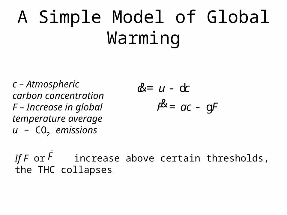
A Simple Model of Global Warming
c u c= - d&
F ac F= - g&
c – Atmospheric carbon concentration F – Increase in global temperature averageu – CO2 emissions
If F or increase above certain thresholds, the THC collapses.
F

Illustration of the Risk Structure
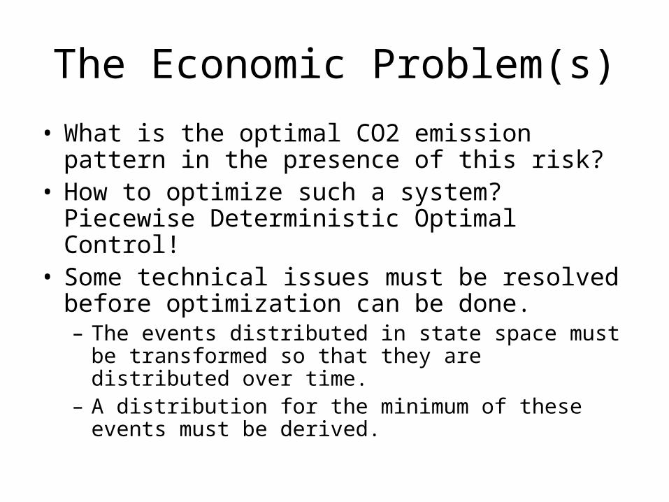
The Economic Problem(s)
• What is the optimal CO2 emission pattern in the presence of this risk?
• How to optimize such a system? Piecewise Deterministic Optimal Control!
• Some technical issues must be resolved before optimization can be done.– The events distributed in state space must be
transformed so that they are distributed over time.
– A distribution for the minimum of these events must be derived.

The Optimization Problem
Climate cost. 0 if THC is OK, G if THC collapses
Cost of reducing emissions below unregulated emission level u0.
0
20
2max dtuu
KEu
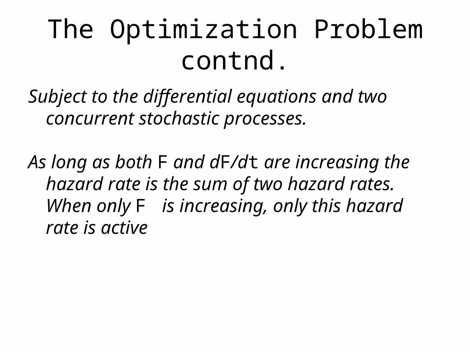
The Optimization Problem contnd.
Subject to the differential equations and two concurrent stochastic processes.
As long as both F and dF/dt are increasing the hazard rate is the sum of two hazard rates. When only F is increasing, only this hazard rate is active

The Hamiltonian for the present problem
First terms are the standardHamiltonian
This term is the expected loss/gain from disaster in the interval (t, t + dt)
ztcJcm
mucuuuK
H mmcc
l
|,,2
20

The Optimal Path

Optimal Time path for Temperature
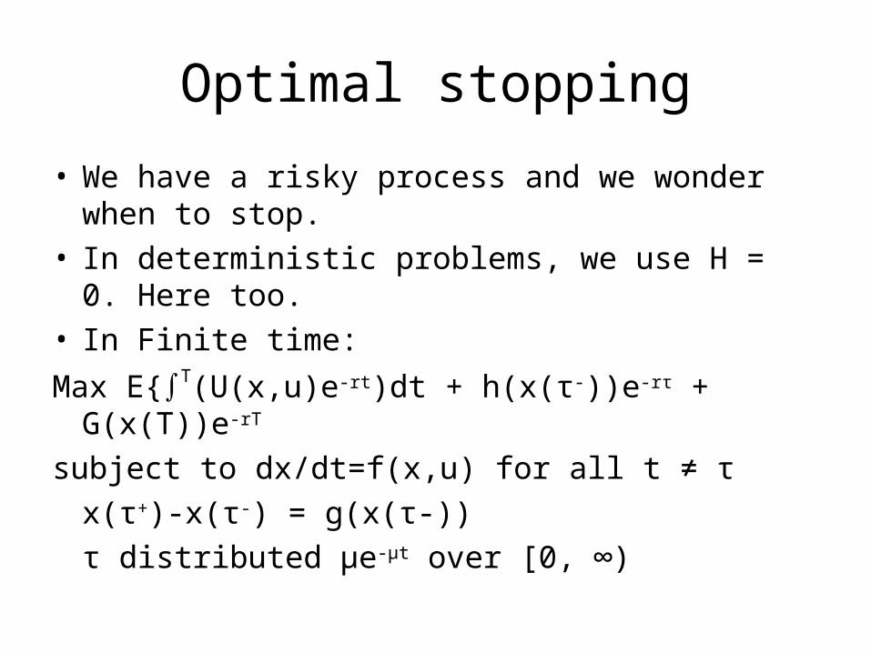
Optimal stopping
• We have a risky process and we wonder when to stop.
• In deterministic problems, we use H = 0. Here too.• In Finite time:
Max E{∫T(U(x,u)e-rt)dt + h(x(τ-))e-rτ + G(x(T))e-rT
subject to dx/dt=f(x,u) for all t ≠ τ
x(τ+)-x(τ-) = g(x(τ-))
τ distributed μe-μt over [0, ∞)

A quick word about the value function
• If we have a scrap value, then we have that J(T,x(T)) = Scrapvalue.
• Intuitively obvious, but needs to be pointed out
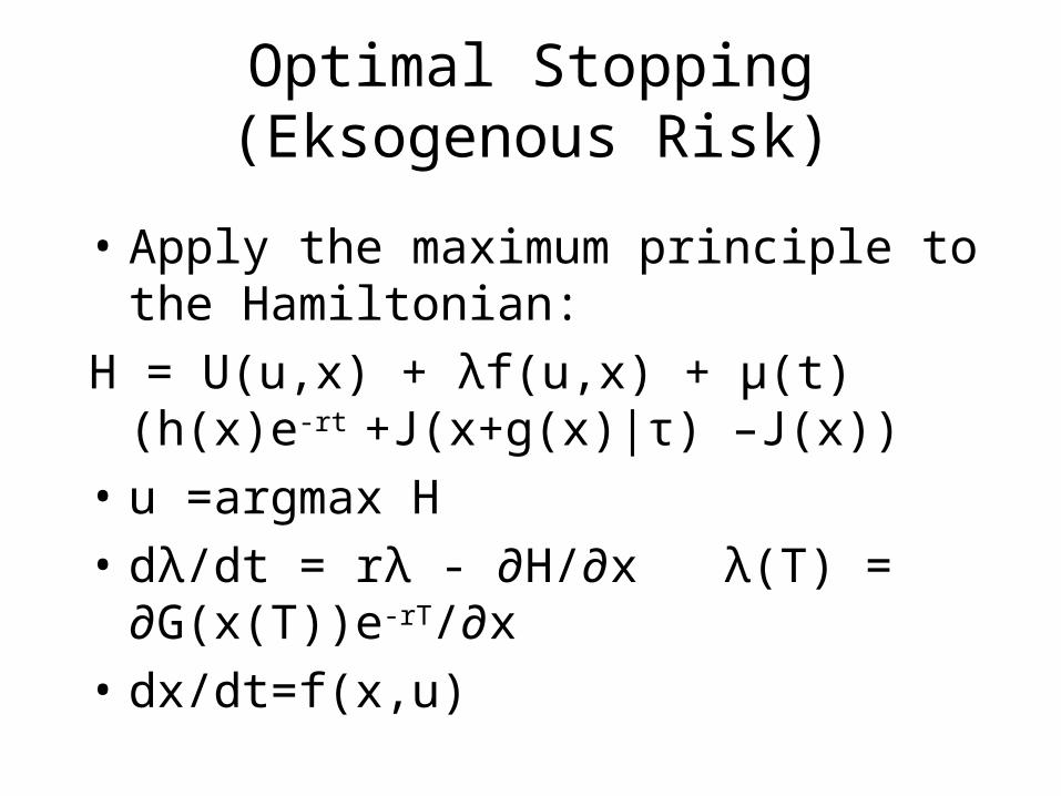
Optimal Stopping (Eksogenous Risk)
• Apply the maximum principle to the Hamiltonian:
H = U(u,x) + λf(u,x) + µ(t)(h(x)e-rt +J(x+g(x)|τ) –J(x))
• u =argmax H
• dλ/dt = rλ - ∂H/∂x λ(T) = ∂G(x(T))e-rT/∂x
• dx/dt=f(x,u)
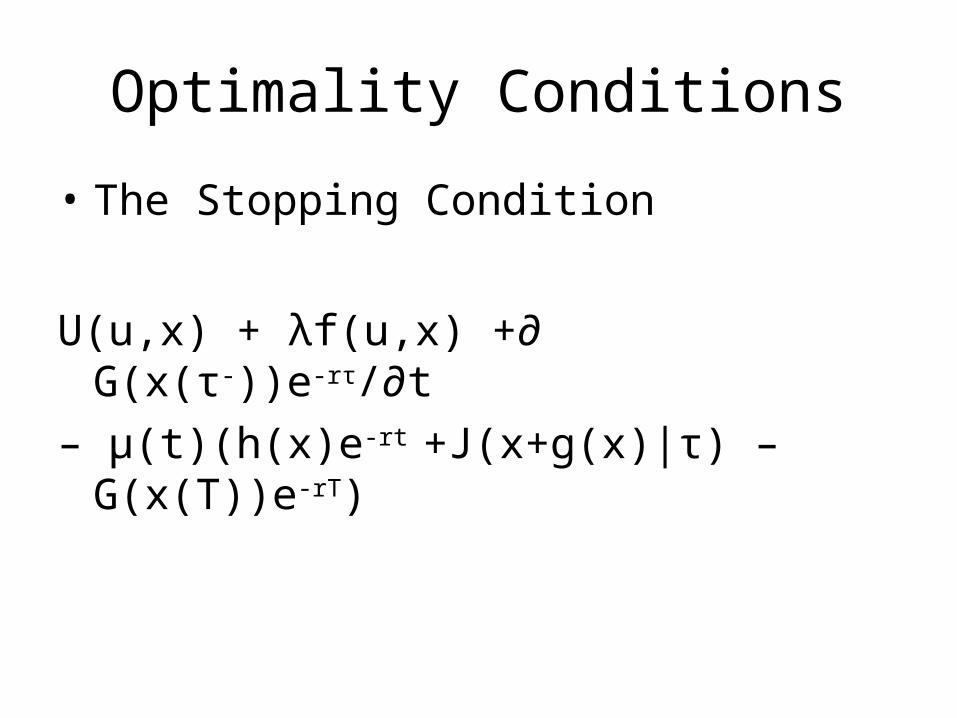
Optimality Conditions
• The Stopping Condition
U(u,x) + λf(u,x) +∂ G(x(τ-))e-rτ/∂t
– µ(t)(h(x)e-rt +J(x+g(x)|τ) –G(x(T))e-rT)
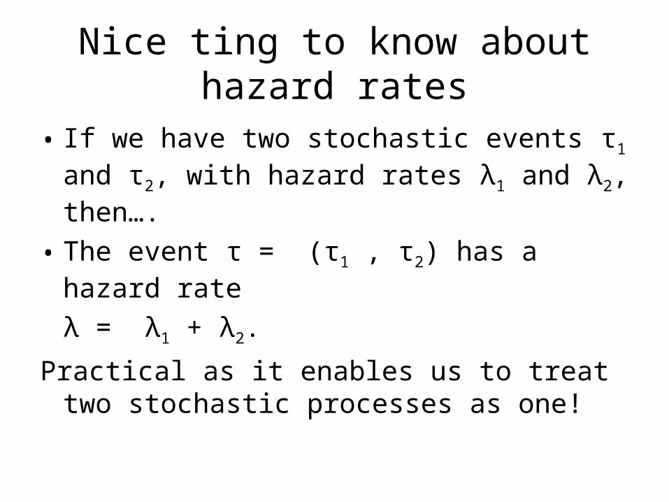
Nice ting to know about hazard rates
• If we have two stochastic events τ1 and τ2, with hazard rates λ1 and λ2, then….
• The event τ = (τ1 , τ2) has a hazard rate
λ = λ1 + λ2.
Practical as it enables us to treat two stochastic processes as one!
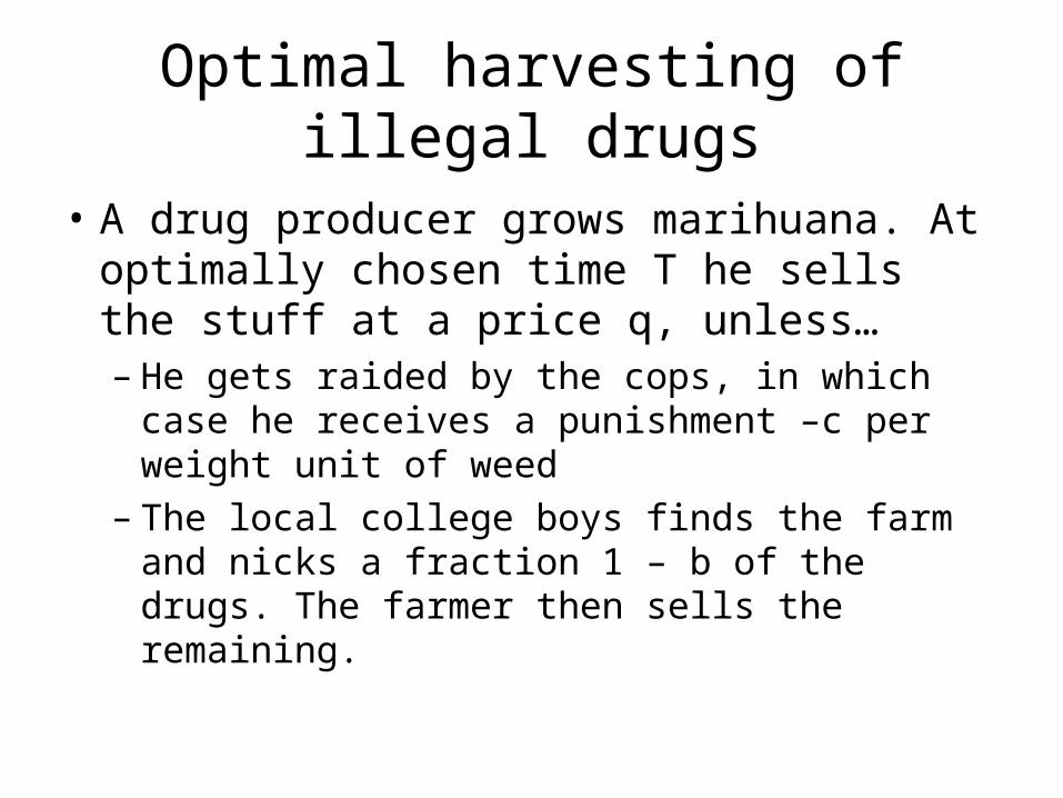
Optimal harvesting of illegal drugs
• A drug producer grows marihuana. At optimally chosen time T he sells the stuff at a price q, unless…– He gets raided by the cops, in which case he
receives a punishment –c per weight unit of weed
– The local college boys finds the farm and nicks a fraction 1 – b of the drugs. The farmer then sells the remaining.
Mathematical formulation
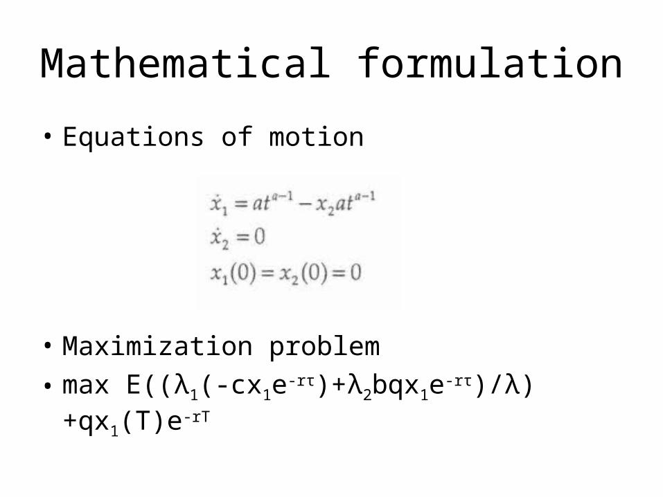
• Equations of motion
• Maximization problem
• max E((λ1(-cx1e-rτ)+λ2bqx1e-rτ)/λ) +qx1(T)e-rT
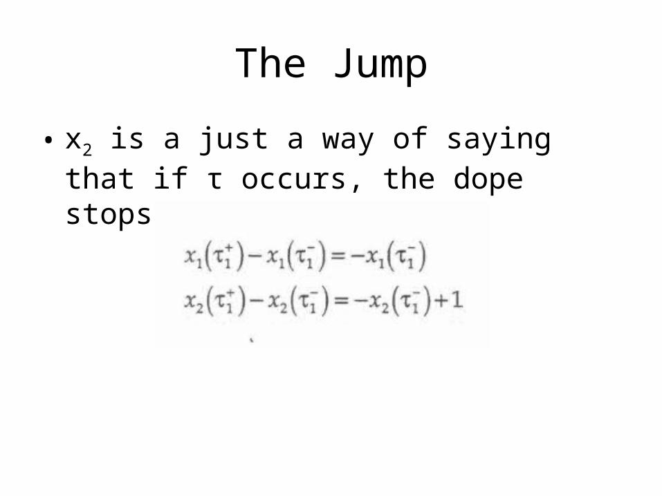
The Jump
• x2 is a just a way of saying that if τ occurs, the dope stops growing
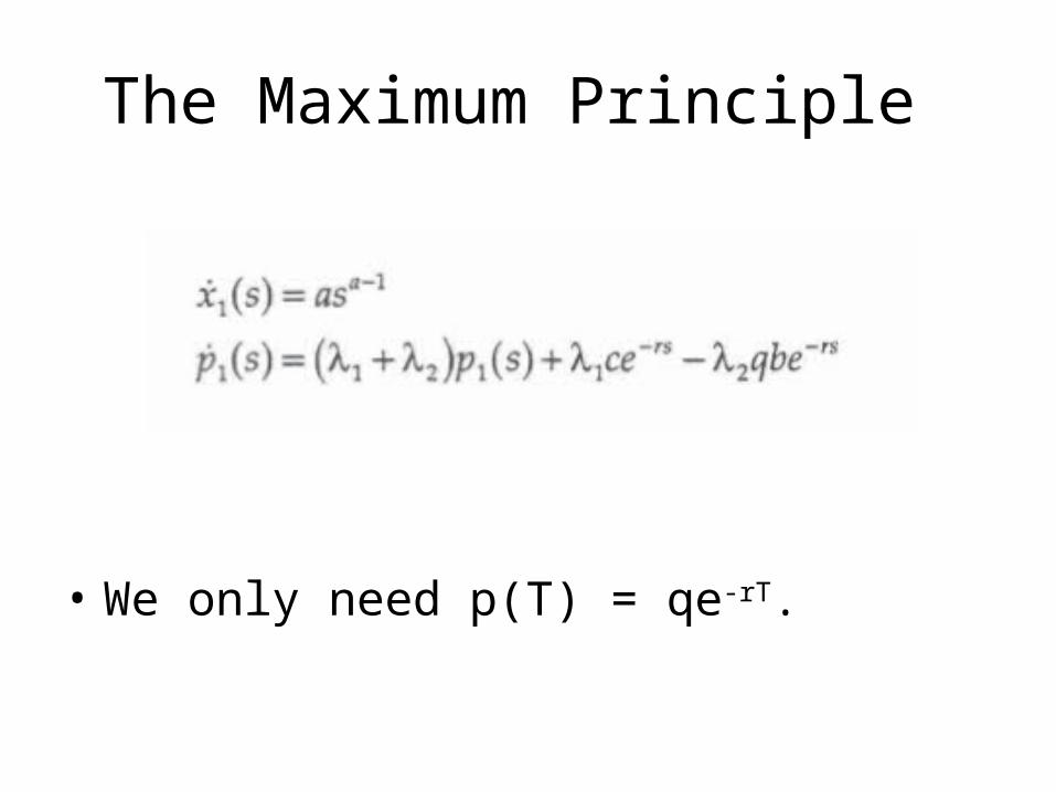
The Maximum Principle
• We only need p(T) = qe-rT.

The Stopping condition
H
Which can be solved and yield:


