Non-linearities, state-dependent prices and thetransmission mechanism of monetary policy

Short title: Non-linearities and state-dependent prices

Guido Ascari∗

University of OxfordUniversity of Pavia

RCEA

Timo Haber†

University of Cambridge

April 23, 2021

Abstract

A sticky price theory of the transmission mechanism of monetary policy shocksbased on state-dependent pricing yields two testable implications, that do nothold in time-dependent models. First, large monetary policy shocks shouldyield proportionally larger initial responses of the price level. Second, in ahigh trend inflation regime, the response of the price level to monetary policyshocks should be larger and real effects smaller. Our analysis provides evidencesupporting these non-linear effects in the response of the price level in aggregateUS data, indicating state-dependent pricing as an important feature of thetransmission mechanism of monetary policy.

Keywords: Sticky prices, state-dependent pricing, monetary policy

JEL Codes: E30, E52, C22

∗Address: Department of Economics, University of Oxford, Manor Road, Oxford OX1 3UQ,United Kingdom. E-mail address: guido.ascari@economics.ox.ac.uk.

†Address: Faculty of Economics, University of Cambridge, Austin Robinson Building, SidgwickAvenue, Cambridge CB3 9DD, United Kingdom. E-mail address: tfh27@cam.ac.uk.

We particularly thank the Editor, Francesco Lippi, and three anonymous referees. We wouldalso like to thank Fernando Alvarez, Efrem Castelnuovo, Luca Dedola, Marco Del Negro, StefanoEusepi, Mishel Ghassibe, Matt Klepacz, Christian Merkl, Gernot Mueller, Anton Nakov, Evi Pappa,Giovanni Pellegrino, Christina Romer, David Romer, Raphael Schoenle, Andrea Tambalotti, par-ticipants to the 6th Workshop in Macro Banking and Finance (U. of Sassari), the Macro MarrakechSixth Workshop in Macroeconomics, the XXI Annual Inflation Targeting Conference of the BancoCentral do Brasil, the EABCN Conference on “Advances in Business Cycle Analysis” in Madrid,the 2019 Padova Macro Talks, the 2019 Annual Congress of the European Economic Association,the EABCN Conference on “New Approaches for Understanding Business Cycles” in Mannheim,the 2019 Annual Meeting of the Central Bank Research Association at Columbia University, andparticipants in seminars at the DNB, the NY Fed, University of Nuremberg for comments andsuggestions.

1 Introduction

The New Keynesian (NK) paradigm is one of the main frameworks for the analysis

of business cycle fluctuations and the effects of monetary and fiscal policy, both among

academic researchers and policy institutions. While there can be alternative mechanisms

for the transmission of monetary policy shocks, price stickiness remains the major reason

why monetary policy has effects on real variables in virtually all NK models. This

pivotal assumption has been substantiated by numerous empirical studies that show that

individual prices do indeed change infrequently (e.g. Bils and Klenow, 2004; Klenow and

Kryvtsov, 2008; Nakamura and Steinsson, 2008; Nakamura, 2008; Eichenbaum et al.,

2011; Nakamura and Zerom, 2010). Moreover, this literature has demonstrated that

microfounded state-dependent models are able to replicate the empirical distribution

of price changes. Unlike time-dependent pricing models, such as Calvo (1983) and

Rotemberg (1982), microfounded state-dependent models of nominal rigidities assume

that the individual firm can change its price, subject to an adjustment cost. Hence,

the frequency of price changes, the number of firms that decide to change their prices

following a monetary policy shock and the size of these changes are endogenous (the

so-called “selection effect”, see Golosov and Lucas, 2007). In particular, these models

predict that individual prices (i) are more flexible in response to large shocks (e.g., Karadi

and Reiff, 2019); (ii) change more frequently when inflation is higher (e.g., Alvarez et al.,

2019).

Some papers find evidence of state-dependent pricing behaviour by investigating the

response of prices at the micro-economic level to a particular event. Hobijn et al. (2006)

document a dramatic increase in restaurant prices in the euro area after the introduction

of the euro and explain it through the lens of a menu cost model. Karadi and Reiff

(2019) document that micro-level price responses to three large value-added tax (VAT)

changes, which occurred in Hungary in 2004 and 2006, were flexible and asymmetrical

1

with respect to positive versus negative tax changes.1 Bonadio et al. (2019) exploit

the Swiss National Bank’s (SNB) decision to discontinue the minimum exchange rate

policy of one euro against 1.2 Swiss francs on January 15, 2015, to analyse the pass-

through of the Swiss exchange rate shock into import product prices from the Euro

area. The empirical literature on exchange rate pass-through is very large. It generally

concerns measuring the extent of the exchange rate pass-through, and, while somewhat

related, it is not concerned explicitly with state-dependent pricing models. Two notable

exceptions are Alvarez et al. (2017) and Alvarez and Neumeyer (2020) that compare the

observed price dynamics at the micro level after a large devaluations to the predictions

of an adjustment cost model of price setting. Alvarez et al. (2017) use monthly data

on Consumer Price Index (CPI) inflation and the nominal exchange rate from a large

number of countries in a panel data analysis. Alvarez and Neumeyer (2020) analyse

several episodes involving large changes in the nominal price of inputs in Argentina

over 2012–2018 by using micro-level price data for the city of Buenos Aires. Alvarez

et al. (2017) is the closest paper to ours because they use aggregate data and they link

explicitly the empirical analysis to the prediction of state-dependent pricing model that

the inflation response should depend on the size of the shock.

Yet, despite the large literature on sticky prices, to the best of our knowledge, there is

surprisingly little direct evidence that aggregate prices behave as state-dependent mod-

els suggest and thus that (i) and (ii) affect the transmission mechanism of monetary

policy in aggregate US data.2 We aim to fill this gap. If staggered prices are of such

paramount importance to the transmission mechanism of monetary policy, and if there

is a significant fraction of state-dependent prices, then the two very general predictions

1Alvarez et al. (2006) and Gagnon et al. (2012) are earlier papers that find significant increases inthe frequency of price changes in the months with VAT tax changes, consistent with state-dependentpricing models.

2As said, the closest reference is Alvarez et al. (2017) who however investigates only prediction (ii)above, use a panel of country and look at exchange rate pass-through interpreting exchange rate move-ments as cost shocks. Veirman (2009) investigates empirically whether the flattening of the JapanesePhillips Curve depends on lower trend inflation, as state dependent models would imply.

2

(i) and (ii) should also emerge in aggregate data. First, large absolute value monetary

policy shocks should lead more firms to adjust their prices, and hence yield a propor-

tionally larger response of inflation, whereas the real effects should be subdued. Second,

the frequency of price changes should be an increasing function of underlying levels of

inflation, that is, prices should be more flexible in a high trend inflation regime than

otherwise. Hence, the higher trend inflation, the larger the response of inflation and the

smaller should be the real effects of monetary policy shocks.

These theoretical results are quite intuitive and general since they derive from a broad

variety of state-dependent sticky price models in the literature. In particular, Alvarez

et al. (2017) show that the impulse response after a monetary shock is size-independent

in time-dependent models, whilst it is not in state-dependent models. In this sense, our

contribution is really a minimal, first-pass test for state-dependent price theories: if state-

dependency is pivotal, aggregate data should exhibit these two features. We take these

two theoretical predictions to US data between 1969 and 2007, applying smooth local

projections (Jorda, 2005; Barnichon and Brownlees, 2019) and the smooth transition

function methodology of Granger and Terasvirta (1993) together with US monetary

policy shocks identified with the narrative method of Romer and Romer (2004). The

empirical methodology of this paper is most closely related to the work of Tenreyro

and Thwaites (2016), focusing on the differential effects of monetary policy in recessions

and expansions. As such, our paper contributes also to the literature about the state

dependent effects of monetary shocks.

Our analysis provides new and statistically significant evidence in favour of state-

dependent pricing models in aggregate US data. First, large absolute value shocks have

disproportionately larger effects on prices on impact, but are less persistent and have

weaker real effects, matching the first theoretical prediction. Second, the impulse re-

sponse functions (IRFs) in the high and low trend inflation regimes are significantly

different for prices and inflation and also in line with the second theoretical prediction of

3

higher price flexibility in the high trend inflation regime. However, for the second predic-

tion, we do not find statistically significant evidence of muted real effects. Importantly,

the non-linearity of the impulse response functions is not due to a different feedback of

monetary policy to inflation in response to small vs. large shocks or in periods of high

vs. low trend inflation. In the Appendix we conduct a comprehensive sensitivity analysis

to establish the robustness of these results, regarding different empirical specifications,

sub-samples, controls, and measures of monetary policy surprises.

Our results are the first ones (to the best of our knowledge) that point towards a

significant presence of state-dependent pricing in the US economy from an aggregate

perspective. Our macro evidence is therefore a useful complement to existing micro

evidence.

2 Theory and Testable Implications

Contrary to early standard time-dependent pricing models (e.g., Fischer, 1977; Taylor,

1979, 1980; Calvo, 1983), microfounded state-dependent pricing models feature endoge-

nous price adjustments triggered by changes in the economic environment. The firms

that decide to change their prices by paying the adjustment costs after a monetary shock

are the ones further off from their optimal price (“selection effect”). Hence, since these

are not random firms and the sizes of the price changes are relatively large, early stud-

ies (Caplin and Spulber, 1987; Golosov and Lucas, 2007) find that the aggregate price

level can mimic a flexible price environment. Nonetheless, later studies investigate the

robustness of this result to various extensions and show that state-dependent models

yield a large degree of aggregate price stickiness and are important for the transmission

mechanism of monetary policy.3

3These extensions are informational costs (Gorodnichenko, 2008; Bonomo et al., 2013; Alvarez et al.,2011), multi-product firms (Alvarez and Lippi, 2014; Midrigan, 2011; Bhattarai and Schoenle, 2014),multiple sectors and intermediate inputs (Nakamura and Steinsson, 2010), or errors in the timing andthe precision of the adjustment (Costain et al., 2019). The same result holds in a variety of state-

4

First Testable Implication: The impulse response functions of inflation

and output to a monetary policy shock should depend on the size of the

shock. If there is a non-negligible fraction of state-dependent price-setters, the impulse

response should be a non-linear function of the size of the shock. The larger the shock,

the larger the number of firms that decide to pay the adjustment costs and change their

prices immediately, such that the reaction of the aggregate price level at short horizon

is increasing in the size of the monetary policy shock (see Alvarez and Lippi, 2014).

Moreover, the effect on the price level should be less persistent, because the larger the

shock, the higher the number of firms that adjust immediately and hence the lower the

number of firms that eventually would change their price as the shock tapers off. The

real effects of monetary policy shocks, instead, are hump-shaped with respect to the size

of the shock, because of two counteracting effects. First, larger shocks, ceteris paribus,

give rise to stronger real effects, just like in a time-dependent model. Second, larger

shocks also increase the number of adjusting firms, strengthening the reaction of the

aggregate price level and thus reducing the real effects. For a small shock, the first effect

prevails, so that both the impact and the cumulative effect on output is increasing in

the size of the shock. For large shocks the opposite occurs. It follows that sufficiently

big shocks should have lower real effects than smaller shocks.4

Second Testable Implication: The impulse response functions of inflation

and output to a monetary policy shock should depend on the average level

of inflation. As outlined in Dotsey et al. (1999) or Costain and Nakov (2011), average

inflation affects the frequency of price adjustments in state-dependent models, because

it erodes a firm’s relative price so that firms adjust prices more frequently. Indeed, the

dependent models that are carefully calibrated to match the main features of retail price microdata(Alvarez et al., 2016; Eichenbaum et al., 2011; Costain and Nakov, 2011, 2019), and, more recently, ofboth the size and frequency of price and wage changes (Costain et al., 2019).

4Alvarez and Lippi (2014) show that the monetary shock that maximises the cumulated effect onoutput (i.e., the area under the impulse response function) is about one-half of the standard deviationof price changes. Costain et al. (2019) show that a similar effect occurs in a model with state-dependentprices and wages.

5

empirical analysis in Alvarez et al. (2019) provides solid evidence of how the frequency

of price changes varies with inflation.5 This evidence implies different impulse responses

to a monetary policy shock in high trend inflation regimes compared to low trend in-

flation regimes. In particular, we should observe a quicker and less persistent reaction

of prices in high inflation regimes. Further, Alvarez et al. (2016) show that in a large

class of sticky-price models, the total cumulative output effect of a small unexpected

monetary shock is inversely related to the average number of price changes per year.6

This theoretical prediction provides the second testable implication.

3 Empirical Methodology

In this Section we describe the data and the empirical methodology used to estimate

smooth impulse responses and conduct inference. We test the two predictions by

analysing the presence of non-linearities in the impulse response functions to a mon-

etary policy shock for large and small shocks, and during high and low trend inflation.

Our empirical methodology follows a growing body of literature employing local projec-

tions (Jorda, 2005) to account for the response to non-linear terms and state-dependency

in empirical impulse responses (e.g. Auerbach and Gorodnichenko, 2012a,b; Caggiano

et al., 2014, 2015; Tenreyro and Thwaites, 2016; Ramey and Zubairy, 2018; Furceri et al.,

2016).

Data The monthly sample for our response variables runs from 1969m1 up to

2007m12, excluding the most recent financial crisis, where monetary policy has been

very different and the zero-lower bound on nominal interest rates has been binding.

5Figure 5 and 6 therein show that the frequency of price changes do not react much for levels ofannual inflation up to 5%, then it starts accelerating and finally it increases linearly for values of annualinflation above 14% with an elasticity of about two-thirds. This is in line with Sheshinski and Weiss(1977)’s adjustment cost model with no idiosyncratic shocks.

6The same holds in a model in which nominal rigidities in both wages and prices are state-dependent(see Figure 11 in Costain et al., 2019), and in a model that allows for temporary price changes, becausefirms can set a price plan, rather than a fixed price as in the standard adjustment cost model (see Figure7 in Alvarez and Lippi, 2020).

6

We analyse three response variables: output, inflation and the nominal interest rate.

The series for output is the industrial production index, for inflation we use personal

consumption expenditure (PCE) inflation, and for the nominal interest rate we use the

effective federal funds rate, all from the Federal Reserve Bank of St. Louis Database

(FRED).7

The main shock variable used in this analysis is based on the narrative analysis of

Romer and Romer (2004). They identify monetary policy surprises by using a narrative

approach to infer the intended federal funds rate at every Federal Open Market Com-

mittee (FOMC) meeting from 1969 onwards. By regressing changes of this intended

rate on Greenbook forecasts they derive a measure of monetary policy surprises that is

arguably exogenous to the Fed’s information set about the future state of the economy.

We utilise this methodology and the extended shock sample until December 2003 by

Tenreyro and Thwaites (2016).

There are a number of other ways of identifying monetary policy surprises, for ex-

ample High Frequency Identification (HFI) (Kuttner, 2001; Gurkaynak et al., 2005;

Barakchian and Crowe, 2013; Gertler and Karadi, 2015) or identification restrictions

in a Vector Autoregression (VAR) (Christiano et al., 1999; Bernanke and Mihov, 1998;

Kim and Roubini, 2000; Uhlig, 2005; Bernanke et al., 2005). We conduct robustness

tests with respect to the latter and find largely similar conclusions.8

Smooth Local Projections We estimate local projection coefficients using the re-

cently developed methodology by Barnichon and Brownlees (2019) to improve accuracy

7The variables are all in natural log levels and then multiplied by 100 except for the federal fundsrate which remains in percentage points. This standard transformation enables the interpretation ofthe strength of the coefficients as approximate percentage points.

8We do not, however, include HFI shocks for two main reasons. First, the available shock seriesare too short for our analysis. Even the backward extension up to 1979 by Gertler and Karadi (2015)omits a significant proportion of the Great Inflation period; a major source of variation in our smoothtransition function. Second, Ramey (2016) argues that these shocks may not be robust to sampleswhere anticipation effects are important. Moreover, (Ramey, 2016, p. 109) shows that the impulseresponse function to HFI shocks can look very different depending on whether one uses a VAR orlocal projections. For example, a contractionary Gertler and Karadi (2015) shock in a local projectionincreases output and leaves the price level largely unchanged whereas it produces the literature standardeffect in their proxy SVAR.

7

and inference over the standard least squares approach.9 With this technique, the im-

pulse response coefficients, i.e. all shock-dependent coefficients, are modelled as linear

combinations of B-spline basis functions. One can then estimate the coefficients of these

linear combinations using generalised ridge estimation, with a penalty parameter that

selects the degree of shrinkage. When the shrinkage parameter is close to zero, the

estimation yields the standard least squares estimates. Conversely, if the parameter is

high, the impulse response is converging to a smooth limit polynomial distributed lag

model. We follow Barnichon and Brownlees (2019) and select the shrinkage parameter

using k-fold cross validation (Racine, 1997).

We also follow Barnichon and Brownlees (2019) on conducting inference. In par-

ticular, in order to take into account potential autocorrelation and heteroskedasticity

we estimate the variance of the coefficients using a modified Newey and West (1987)

estimator, corrected for the penalty parameter. We use the resulting variance matrix to

construct confidence intervals and t-statistics in the ordinary way. We provide further

details on this and the estimation technique as a whole in the Appendix.

4 Results

This Section presents the main results regarding the two testable implications above.

4.1 Implication 1: Size-dependent effects of monetary policy

shocks

Non-linear local projections. In order to test the size-dependence of impulse re-

sponses we consider the following non-linear local projection:

yt+h = αh + τht+ βhet + ζh(et · |et|) +K∑k=1

γh,kwt,k + vt+h, (1)

9We provide the results with standard least squares coefficients in the Appendix.

8

which is estimated for h = 0, 1, . . . , H. We set H = 48 which corresponds to an impulse

response horizon of four years. yt+h denotes the variable of interest, in our case either

the industrial production index, PCE inflation or the federal funds rate. et are the nar-

rative Romer and Romer (2004) shocks. wt,k denotes the kth control variable and vt+h

the estimation error, possibly heteroskedastic and serially correlated. The set of control

variables includes up to two months of lags of industrial production, PCE inflation and

the federal funds rate. Moreover, we follow Ramey (2016) and include contemporaneous

values of the industrial production index and PCE inflation. This is equivalent to as-

suming recursiveness between the three different variables of interest since inflation and

industrial production can contemporaneously affect the federal funds rate but not vice

versa.10

While the coefficient βh captures the linear component, the coefficient ζh on the abso-

lute value interaction term accounts for non-linearities in the impulse response function

due to the size of the shock. The interaction term, (et · |et|), magnifies the size of the

shock, but it keeps the same sign of the shock. Hence, contrary to a simple quadratic

term, it isolates the pure effect of a change in the size of the shock. If ζh has the same

sign of βh then the non-linear interaction term amplifies the linear effects of the impulse

response. On the contrary, if ζh has the opposite sign to βh, it counteracts the linear

impulse response, possibly even tilting the overall effect from one sign to another for

large enough shocks. Whenever ζh = 0 the impulse response function is linear with

respect to the shock size.

Therefore, ζh is the main coefficient of interest to test our first theoretical prediction.

Let yt signify prices, and assume a large monetary contraction, i.e., a positive value of et.

Large monetary policy shocks should induce a more price-flexible impulse response func-

tion of the price level and inflation. If firms exhibit state-dependent pricing we should

10As Ramey (2016) points out, relaxing this assumption would otherwise lead to a number of puzzles.A contractionary monetary policy shock would actually be expansionary for about a year and producea very pronounced price puzzle.

9

see a negative ζh at small horizons as we expect βh to be close to zero or negative. This

would mean that firms decrease prices quicker and so prices decline disproportionately

at small horizons. Furthermore, we would then expect to see a positive ζh at larger hori-

zons, weakening the price response, as more firms have already changed prices earlier.

Consequently a combination of a negative ζh at small horizons, as more firms change

prices right away, and a positive ζh at larger horizons, as persistence is lower due to ear-

lier price changes, would speak in favour of state-dependent pricing as a valid aggregate

propagation mechanism of monetary policy shocks.

Coefficient estimates. The resulting coefficients from estimating local projection

(1) for PCE inflation, industrial production and the federal funds rate are reported in the

panels of Figure 1. The solid black line plots the coefficients of the linear term, βh, and

the dashed-dotted green line plots the ones of the non-linear absolute value interaction

term, ζh, together with their 90% confidence interval bands.

The linear terms in the projection deliver a familiar picture in the top panel. After a

positive (contractionary) monetary policy shock the linear coefficients yield an initially

muted response of inflation followed by significant decline thereafter. There is an initial

positive response which is however not significant on impact and marginally so for just

few months in the initial year. Hence, the response displays a slight price puzzle, if we

were to consider only the linear effect.

The non-linear effects implied by the absolute value interaction coefficients are sup-

porting the theoretical predictions. Initially the ζh coefficients are negative, counteract-

ing the price puzzle as the shock size increases and indicating a quicker negative response

of inflation on impact. Moreover, after about two years, the coefficients on the non-linear

term turn positive (and increase), meaning that inflation responds less to a large shock

at long horizons. Hence, the evidence suggests that inflation has a stronger reaction at

short horizons and a weaker one at long horizons. This is consistent with theoretical

models of state-dependent pricing as, for large shocks, more firms adjust immediately

10

and hence less adjust later on. Most importantly, the confidence interval shows that the

coefficients are statistically significant for most of the horizons.

The other two panels report the results for the linear coefficient in the industrial

production and federal funds rate local projection. These results are in line with the

theoretical implications from the literature. The linear output coefficient starts to fall

(after a small, positive, but not significant, initial response), reaching its trough two and

a half years after the shock, and then recovers. The linear federal funds rate coefficient

exhibits a hump-shaped response and remains positive for more than two years after the

shock before turning negative.

Further, the green dashed-dotted line in the middle panel shows that the output

response supports the predictions of state-dependent pricing models. The coefficients

on the non-linear term in (1) are negative at the beginning, counteracting the small

positive output response, and then turn positive at longer horizons. As such, the ζh

estimate counteracts the linear response for both short and long horizons, flattening the

overall response of output. While the top panel shows that large monetary policy shocks

predict a higher degree of price flexibility, the middle panel shows that larger monetary

policy shocks have weaker real effects. Again, the confidence band indicates that the

non-linear interaction term is statistically significant.

It is crucial to note that these results are not due to a stronger response of mone-

tary policy, because the coefficients of the federal funds rate on the non-linear term in

the bottom panel are negative for most of the short to medium horizons, suggesting a

proportionally weaker response of monetary policy to a larger shock.

In sum, prices exhibit a non-linear, size-dependent impulse response function, re-

acting strongly at short and weakly at long horizons for large shocks. Coherently, the

output response seems to be smaller, and monetary policy feedback does not seem to

drive the above results. Hence, we interpret these findings as evidence in favour of

state-dependent prices as an important propagation mechanism of monetary policy, as

11

larger shocks induce more firms to change prices early, thus reducing the real effects of

a monetary shock.

Impulse Response Functions. In order to further assess and clarify the impor-

tance of the non-linear effect, Figure 2 compares IRFs to different shock sizes of all three

headline variables over a four year horizon. It depicts the impulse responses for a 25

(dashed blue line), 100 (solid black line) and 200 (dashed-dotted green line) basis point

shock, where each impulse is standardised by dividing it by the respective shock size.

The standardised IRFs clearly visualise that inflation responds more strongly to a larger

shock at short horizons, but then the reaction is less persistent, so that the response is

weaker at long horizons, as theory would predict. First, the larger the shock, the quicker

inflation decreases. Second, for a large enough shock, the initial price puzzle on impact

tend to disappear.11

The response of output to small and large shocks also supports the theoretical pre-

diction. The standardised IRFs show that the trough in output is smaller relative to

the size of the shock, consistent with the behaviour of the responses of inflation. Re-

call that, in state-dependent models, there are two opposite effects on output. First,

the larger the shock, ceteris paribus, the larger the response of output. This standard

effect is the only one present also in time-dependent pricing models. Second, the larger

the shock, the greater the number of firms that adjust the price, hence the larger the

response of inflation and the smaller the one of output. This second effect is absent in

time-dependent models. Therefore, the output response to a large shock is proportion-

ally flatter in state-dependent models, because of this second effect that counteracts the

first one. By showing the response relative to the size of the shock, the standardised

11Figure H5, discussed in Appendix C.3, depicts the unscaled (i.e., non standardised) impulse re-sponses for a 25 basis point shock and a 200 basis point shock and their 90% confidence intervalcalculated with the Delta method, respectively (see Appendix for details). The response of inflation toa 200 basis point shock is firstly not significantly different from zero and then significantly negative,while it is positive for some months for a 25 basis point shock (even if only marginally significantly).Consequently, a sufficiently large shock counteracts the small linear coefficient and switches the sign ofthe overall impulse response of inflation, removing a potential price puzzle.

12

IRFs isolate the second effect, thus, revealing whether there is a significant effect coming

from state-dependent pricing. Finally, the standardised IRFs also highlight the effect

of state-dependent pricing both on the scale, i.e., decreasing real impact as the shock

gets larger, and on the timing, i.e., arriving sooner with larger shocks, of the response

of output and inflation to the policy shocks.

To strengthen our point, Table 1 shows the cumulative effect of a monetary policy

shock on inflation (i.e. the PCE deflator) and on output for small and large shock,

standardised by the size of the shock, and their significance levels, for different horizons:

1, 12, 24, 36 and 48 months.12 Coherently with the theoretical predictions, prices move

significantly downwards on impact for large shocks, while they do not for small shocks.

Due to this lagged and inertial behaviour in case of small shocks, the cumulative response

of the price level after four years is almost doubled, relative to the size of the shock,

compared with the response to a large shock. The cumulative response of output reflects

the one of the price level. The initial response of output is sharper for large shocks, but

the cumulative drop in output after four years is about 80% proportionally larger for

small shocks.

Finally, the last row in Figure 2 again illustrates that the empirical results are not

due to the different behaviour of monetary policy after a large shock. The standardised

IRFs of the Fed funds rate is milder for larger shocks, relative to shock size, and hence,

if anything, it would play against our results.13

Figure 2 and Table 1 reinforce our previous empirical results on the significant size-

dependent effects of monetary policy shocks. Large shocks induce firms to change prices

early on and thus reduce the real effects of such a monetary shock, in accordance with

our first theoretical prediction.

12We simply cumulate the point estimates from the standard least squares estimation and statisticsusing the Delta method.

13Moreover, the response of the federal funds rate is statistically different (in the first year) betweenthe 25 verus 200 basis points shock (see Figure H5 in the Appendix).

13

4.2 Implication 2: Trend inflation-dependent effects of mone-

tary policy shocks

Smooth transition local projections. We use smooth transition local projections

to test whether the impulse responses after a monetary policy shock are different in

high and low inflation regimes. Auerbach and Gorodnichenko (2012b) and Tenreyro and

Thwaites (2016) popularised this method, and we follow their approach to a large extent.

The impulse response of the variable of interest yt at horizon h in state s = HI,LO14

to a unitary structural shock et is the estimated coefficient βsh in:

yt+h = τht+ F (zt)(αHIh + βHIh et +

K∑k=1

γHIh,kwt,k)

+(1− F (zt))(αLOh + βLOh et +

K∑k=1

γLOh,kwt,k) + ut+h, (2)

for h = 0, 1, ..., H. Again, our set of controls {wt,k}Kk=1 includes the contemporaneous

values of industrial production and PCE inflation and up to two month lags of indus-

trial production, PCE inflation and the effective federal funds rate. F (zt) is a smooth

transition function which indicates the state of the economy (Granger and Terasvirta,

1993). We use a logistic function with the following form:

F (zt) =exp (γ (zt−c)

σz)

1 + exp (γ (zt−c)σz

)∈ [0, 1]. (3)

If state-dependent prices are an important aggregate propagation mechanism we would

expect βHIh to be statistically significantly more negative than βLOh for the response of

the price level and inflation, especially at short horizons. Prices should be more flexible

and so react both more quickly and strongly to monetary policy shocks in a high inflation

regime.

14HI stands for high inflation, LO for low inflation.

14

In the main specification of our smooth transition function local projection, i.e.,

equation (2), the state variable zt represents smoothed personal consumption expendi-

ture (PCE) inflation, so we take a 24 month centered moving average (MA) to capture

trend inflation.15 We set γ = 5 as this gives an intermediate degree of regime switching

intensity. This is relatively standard in the literature and also fits our inflation data well.

Finally, c corresponds to the 75th percentile of the historical trend inflation distribution.

This is equivalent to assuming that about 70% of the time trend inflation is classified

as negligible (i.e. F (zt) ∈ [0, 0.1]) and 30% of the time there is some trend inflation (i.e.

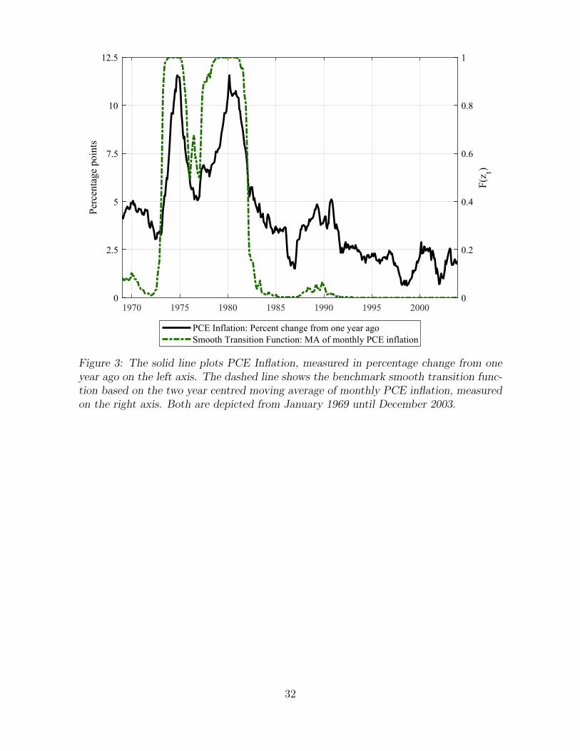
F (zt) ∈ (0.1, 1]). Figure 3 displays the resulting smooth transition function, F (zt). The

solid black line, measured on the left vertical axis, shows PCE inflation on an annual

basis. The green dashed line, measured on the right vertical axis, depicts the smooth

transition function based on our MA-filtered measure of PCE inflation. The period

of the Great Inflation from around 1974 to 1983 is characterised by two pronounced

spikes of inflation of up to 11%. The smooth transition function reaches 1 around these

two peaks and stays above 0.4 for the entire period of the Great Inflation, classifying

the latter period mostly as a high inflation regime. We take this to be a reasonable

approximation for periods of high and low trend inflation in the United States.16

Coefficient estimates. The panels of Figure 4 display the coefficient from esti-

mating equation (2) for each response variable (by row). The first column shows the

point estimates of the βih coefficients for the linear (solid black line), the high inflation

(dash-dotted green line) and low inflation (dashed blue line) regimes. Column two and

three depict the impulse responses conditional on the high inflation and low inflation

regime respectively, with their 90% confidence intervals. The last column displays the

t-statistic that tests the null of equality of the high and low inflation regime coefficients,

15The moving average is our benchmark smoothing procedure. However, the results from the localprojections are very similar with a HP-Filter (λ = 14400) smoothing procedure, see the Appendix.

16This calibration is also in accordance with Alvarez et al. (2019) who show that the frequency ofprice changes starts increasing significantly from annual inflation rates of 5%. Our smooth transitionfunction indicates a value of approximately 0.5 with such an annualised inflation rate.

15

i.e., βHIh = βLOh , where the grey area represents the 90% z-values. A positive value means

that the high inflation response is larger whereas a negative value of the t-statistic indi-

cates the opposite. First, the linear terms for PCE inflation in the top left panel show

the familiar picture in the literature. PCE Inflation declines eventually, after an initial

positive response, which however is not statistically significant. Second, inflation in a

high inflation regime declines right away on impact after a contractionary monetary

policy shock. On the contrary, the impulse response function in a low inflation regime

exhibits a price puzzle for about one year, which is marginally statistically significant

only for few months. This suggests that in this regime firms are not willing to change

price as frequently, so the price level stays persistently around zero for a longer pe-

riod. Moreover, at long horizons the response is smaller in a high trend inflation regime.

Again, this is consistent with the idea that the effect is less persistent in a high inflation

regime, because more firms adjust on impact after the shock. Third, the last column

shows that the responses of inflation in a high and low inflation regime are statistically

significantly different both at short and at long horizons. We interpret these results as

evidence in favour of state-dependent prices models as key propagation mechanism of

monetary policy shocks, because they predict a faster, and less persistent, reaction to a

monetary disturbance in a high trend inflation regime. This is exactly what the impulse

response functions show.

The first panel in the second row shows that the IRFs for output exhibit the usual

hump shaped dynamics. Output reacts with a larger delay in a low inflation regime

compared to a high inflation regime, but this reaction is stronger and reaches a trough

after two years which is roughly twice as deep as the one in a high inflation regime. The

difference in the IRFs between the two regimes however is not statistically significant,

so that we do not find evidence for our second theoretical implication regarding output.

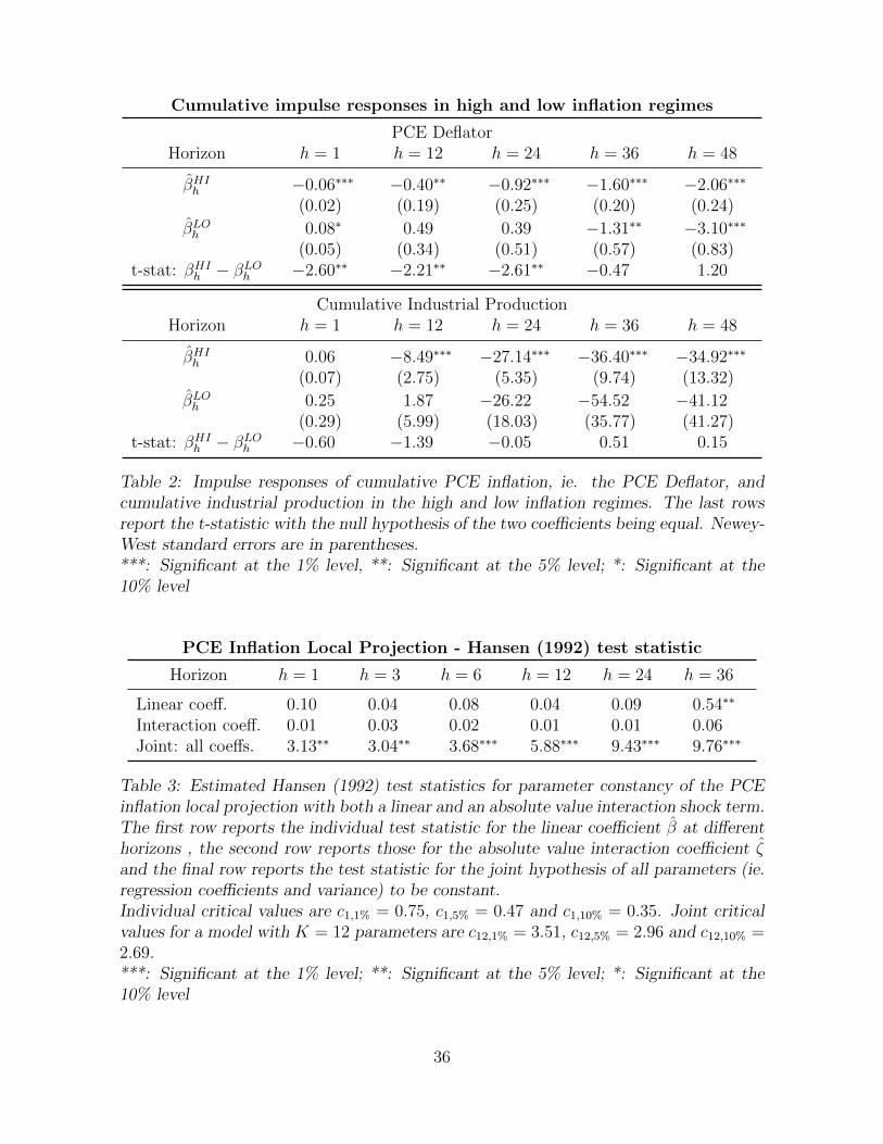
Table 2 displays similar results for the cumulated IRFs of inflation and output at different

horizons. Prices drop from the outset in a high inflation regime, while the reaction is

16

sluggish in a low inflation regime. However, the latter is more persistent so that it

eventually catches up and overtakes the cumulative drop in a high inflation regime, so

that the cumulative drop after four years is 50% higher. The difference in the initial

response, up to two years, is statistically significant providing supporting evidence for

state-dependent pricing. This is not the case for the cumulative response of output, that

is both not significant for low inflation regimes and not statistically different between

low and high inflation regime. Again, the point estimates are in line with the theoretical

prediction, but the standard errors get so large (especially for the low inflation regime,

as evident also form Figure 4) that these differences are not significant.

Finally, the panels in the third row show that the interest rate increases after a mon-

etary policy shock and stays positive for about two years, in the linear case and low

inflation regime, while for only one year in the high inflation regime. Thus, monetary

policy initially reacts differently to a shock in the two regimes, and these differences are

statistically significant for the first two years. In a high inflation regime, the nominal

interest rate initially reacts more, but then it decreases much faster than in a low infla-

tion regime. While one might argue that this pattern may explain the initially quicker

reaction of the price level in the high inflation regime, prices in the low regime react

considerably more sluggishly even though the interest rate is positive for a longer period

of time. Indeed, the last column shows that for most of the IRFs the coefficients in

the low inflation regime are larger than the ones in a high inflation regime, perhaps sig-

nalling a stronger endogenous feedback of monetary policy in response to the shock (as

also evident from the IRFs in column one). On the one hand, it would be hard to argue

that the different monetary policy behaviour is driving the different response of prices

between the high and low inflation regimes. On the other hand, the fact that the path

of the federal funds rate after the initial monetary contraction is different across the two

regimes blurs the comparison, possibly explaining why the evidence for the differences

in output responses is not statistically significant.

17

To conclude, we find evidence in favour of state-dependent prices regarding our sec-

ond testable implication with respect to the behaviour of inflation. Our results show

that in a high trend inflation regime, inflation declines right away after a policy shock,

and there is no price puzzle, as theory predicts. Moreover, inflation is more persistent

in a low inflation regime, despite the interest rate staying positive for a longer amount

of time. Regarding the response of output, however, the point estimates are coherent

with the theoretical prediction, but the differences between the high and low inflation

regime are not statistically significant.

5 Robustness

This Section reports the results of two particularly important robustness exercises re-

garding our local projection estimates. We conduct comprehensive robustness checks

on many other dimensions, that we confine to the Appendix and we briefly summarise

below.

5.1 Stability

It is crucial for our analysis to be relatively confident that the non-linear and state-

dependent dynamic behavior of the impulse response functions of output and inflation

is not driven by a feedback effect of monetary policy.17 To show that monetary policy

feedback plays a limited role with respect to large and small shocks, we check if inflation

coefficients with respect to the linear and absolute value interaction term do not exhibit

structural breaks when monetary policy conduct may have changed. If these estimates

stay stable over a variety of monetary policy regimes throughout time then we can reject

17As discussed in section 4.1, several of our results seem to contradict this possibility. For example,monetary policy seems to react weakly after a large shock whereas prices react by more at the beginningof the horizon. The same applies to a large extent to the test of the second implication in section 4.2as the funds rate stays positive for longer in the regime where prices seem to be more sticky. Thesepatterns seem to indicate that the dynamics of inflation and output are not defined by the reaction ofmonetary authorities only.

18

the thesis of monetary feedback driving the result of size-dependent effects.

We apply the Hansen (1992) stability test to the coefficients in the local projection (1)

for PCE inflation. This test has locally optimal power and needs no a priori assumption

concerning the breakpoint. Furthermore, this test is robust to heteroskedasticity, a

potential concern in this analysis. Table 3 shows the results for the two coefficients of

interest and the joint test for parameter stability at a 1, 3, 6, 12, 24 and 36 month

horizon for our PCE inflation local projection.18 We cannot reject the null of individual

parameter constancy for neither the linear nor the absolute value interaction coefficients

at these horizons (with the exception of the linear coefficient at 36 month horizon).

However, the joint test statistic does indicate a rejection of the null that all parameters

in the local projection are constant. This suggests that, even though the dynamic

feedback of monetary policy via lagged control values may have changed throughout

time, the shape and non-linearity of the impulse response after a monetary policy shock

has stayed relatively constant throughout the sample. The same results hold for the

linear and interaction coefficients when the dependent variable is either the industrial

production or the Fed Funds rate (see Appendix).19

5.2 Excluding the NBR targeting period

Coibion (2012) and others have suggested that the exclusion of the NBR targeting period

October 1979 and September 1982 can account for a difference in results between the

Romer and Romer (2004) and VAR approach. Critically, the largest absolute monetary

shock values lie in this period and may thus play a significant role for the conclusion on

18For a test on an individual coefficient, we can reject the null of parameter constancy at the 5%significance level, if the relevant test-statistic is larger than the asymptotic critical value of 0.47. Thenull hypothesis is that each coefficient in (1) is constant and the respective distribution is non-standardand depends on the number of parameters tested for stability. The intuition is that under the nullhypothesis the cumulative sums of the first-order conditions from the estimation will have mean zeroand wander around zero. However, under the alternative hypothesis of parameter instability, thesefirst-order conditions will not be mean zero for parts of the sample and so the test statistic will be large,leading us to reject the null (see Appendix).

19These results substantiate the visual impression from the plots of the recursive estimation of thelocal projection coefficients displayed in the Appendix.

19

our first implication. In order to account for this suggestion we exclude this part of the

shock sample, modifying the non-linear local projection equation (1) by interacting the

linear and the non-linear coefficient with a time-dummy that takes a value of 1 for the

sample between October 1979 and September 1982 and 0 otherwise. As in Figure 2, the

three rows in Figure 5 display the IRFs for this specification for PCE inflation, industrial

production and the Fed Funds rate, respectively, for both the coefficients of the linear

term, βh (green, solid line), and the ones on the non-linear absolute value interaction

term, ζh (blue, dashed line). The impulse response coefficients are qualitatively similar

to the benchmark results. The results, however, change somewhat both in terms of

magnitude and, especially, in terms of significance, particularly so for the interaction

coefficients. This is hardly surprising. The reduced sample does not include the large

shocks of the NBR targeting period, and it features low sample variation with values

mostly below 1. Hence, the non-linear effects of large shocks are more difficult to identify,

inducing wide confidence intervals.

5.3 Other robustness checks

The Appendix presents comprehensive robustness checks. It displays the plots of the

recursive estimates of the local projection coefficients in (1), to further visually inspect

their stability. Besides, results are robust to a different specification of the non-linear

terms in (1), that includes a squared and a cubed term for the shock value, rather than

the absolute value interaction term.

Results for the smooth transition local projections (2) are robust to: 1) changes in γ

and c; 2) using HP-filtered inflation for z; 3) using a model based trend inflation measure

from Ireland (2007).

Finally, the estimates of the coefficients in both (1) and (2) are also robust to: 1)

using the CPI instead of the PCE; 2) using quarterly data with GDP as the output

measure; 3) including as controls: (i) the commodity price index, (ii) the corporate

20

bond credit spread by Gilchrist and Zakrajsek (2012) to control for financial frictions,

(iii) proxies for fiscal policy using either measure of excess returns on stocks of military

contractors from Fisher and Peters (2010) or the exogenous tax changes from Romer

and Romer (2010); 3) different measures of shocks obtained from non-linear models: (i)

from the Romer and Romer (2004) regression using the smooth transition function; (ii)

from a smooth transition VAR; 4) including leads and lags of the shocks to control for

potential autocorrelation and misspecification as suggested by Alloza et al. (2019).

6 Conclusion

The assumption of sticky prices lies at the very center of the current workhorse model for

the analysis of business cycle fluctuations and, particularly, monetary policy effects. The

literature features two type of sticky price models: time-dependent and state-dependent

prices. A sticky price theory of the transmission mechanism of monetary policy shock

based on state-dependent pricing yields two testable implications, that do not hold in

time-dependent models; the impulse response function of the aggregate price level and

inflation should be more flexible both after a large shock and during high trend inflation

regimes. Employing the methodology of local projections, we tested these predictions

on aggregate US data. We found some evidence in favour of state-dependent models

of price stickiness rather than time-dependent ones. With regards to the response to

large shocks, the coefficient of the absolute value interaction shock projections matched

our theoretical prior, both in terms of output and inflation. When the NBR targeting

period of US monetary policy, October 1979 and September 1982, is taken out of the

sample, our results loose statistical significance, because too little variation is present

to identify the non-linear effect and the significance bands becomes very wide. The

empirical investigation during large trend inflation regimes also showed that inflation

reacts significantly more quickly to a monetary policy shock in times of high trend

21

inflation. In this case, the evidence for output is not significant, however, the point

estimates behave according to the theoretical predictions. Furthermore, the Appendix

shows that the results are robust to a very large variety of robustness tests.

Our results are the first ones (to the best of our knowledge) that point towards a

significant presence of state-dependent pricing in the US economy using aggregate data.

Our macro evidence is a useful complement to the large empirical literature on individ-

ual firm price micro data. Hence, ‘Prices are sticky after all’ - just as recent literature

has shown (Kehoe and Midrigan, 2015) - but less so when shocks are large or inflation is

high. These results are in line with what would be expected if state-dependent pricing

played a significant role in the US economy. This supports the theoretical implication

that the frequency of changing prices is, at least to some extent, endogenous to the

economic environment, as in Alvarez et al. (2017). So, although the Calvo (1983) model

may work quite well for “normal” times, when considering situations where high-trend

inflation is present or large shocks are likely, a state-dependent sticky price framework

that accounts for these phenomena seems more appropriate (as e.g., Alvarez and Lippi,

2014; Alvarez et al., 2016; Costain and Nakov, 2011, 2019; Costain et al., 2019).

Guido Ascari, University of Oxford, University of Pavia and RCEA

Timo Haber, University of Cambridge

22

References

Alloza, M., Gonzalo, J. and Sanz, C. (2019). “Dynamic effects of persistent shocks”,

Banco de Espana, Working Paper.

Alvarez, F., Beraja, M., Gonzalez-Rozada, M. and Neumeyer, P.A. (2019). “From Hyper-

inflation to Stable Prices: Argentina’s Evidence on Menu Cost Models”, The Quarterly

Journal of Economics, vol. 134(1), pp. 451–505.

Alvarez, F., Le Bihan, H. and Lippi, F. (2016). “The Real Effects of Monetary Shocks in

Sticky Price Models: A Sufficient Statistic Approach”, American Economic Review,

vol. 106(10), pp. 2817–2851.

Alvarez, F. and Lippi, F. (2014). “Price Setting With Menu Cost for Multiproduct

Firms”, Econometrica, vol. 82(1), pp. 89–135.

Alvarez, F. and Lippi, F. (2020). “Temporary Price Changes, Inflation Regimes, and the

Propagation of Monetary Shocks”, American Economic Journal: Macroeconomics,

vol. 12(1), pp. 104–52.

Alvarez, F., Lippi, F. and Paciello, L. (2011). “Optimal Price Setting With Observation

and Menu Costs”, The Quarterly Journal of Economics, vol. 126, pp. 1909–1960.

Alvarez, F., Lippi, F. and Passadore, J. (2017). “Are State and Time Dependent Models

Really Different?”, in (M. Eichenbaum, E. Hurst and J. A. Parker, eds.), NBER

Macroeconomics Annual, pp. 379–457, vol. 31, University of Chicago Press.

Alvarez, F. and Neumeyer, P.A. (2020). “The Pass-Through of Large Cost Shocks in

an Inflationary Economy”, in (J. G. Gonzalo Castex and D. Saravia, eds.), Changing

Inflation Dynamics, Evolving Monetary Policy, pp. 7–48, chap. 2, Santiago, Chile:

Banco Central de Chile.

Alvarez, L.J., Dhyne, E., Hoeberichts, M., Kwapil, C., Le Bihan, H., Lunnemann, P.,

Martins, F., Sabbatini, R., Stahl, H., Vermeulen, P. and Vilmunen, J. (2006). “Sticky

23

Prices in the Euro Area: A Summary of New Micro-Evidence”, Journal of the European

Economic Association, vol. 4(2-3), pp. 575–584.

Auerbach, A.J. and Gorodnichenko, Y. (2012a). “Measuring the Output Responses to

Fiscal Policy”, American Economic Journal: Economic Policy, vol. 4(2), pp. 1–27.

Auerbach, A.J. and Gorodnichenko, Y. (2012b). “Fiscal Multipliers in Recession and

Expansion”, in (A. Alesina and F. Giavazzi, eds.), Fiscal Policy after the Financial

Crisis, pp. 63–98, chap. 2, University of Chicago Press.

Barakchian, S.M. and Crowe, C. (2013). “Monetary policy matters: Evidence from new

shocks data”, Journal of Monetary Economics, vol. 60(8), pp. 950–966.

Barnichon, R. and Brownlees, C. (2019). “Impulse Response Estimation by Smooth

Local Projections”, The Review of Economics and Statistics, vol. 101(3), pp. 522–530.

Bernanke, B.S., Boivin, J. and Eliasz, P. (2005). “Measuring the Effects of Monetary Pol-

icy: A Factor-Augmented Vector Autoregressive (FAVAR) Approach”, The Quarterly

Journal of Economics, vol. 120(1), pp. 387–422.

Bernanke, B.S. and Mihov, I. (1998). “Measuring Monetary Policy”, The Quarterly

Journal of Economics, vol. 113(3), pp. 869–902.

Bhattarai, S. and Schoenle, R. (2014). “Multiproduct firms and price-setting: Theory

and evidence from U.S. producer prices”, Journal of Monetary Economics, vol. 66,

pp. 178 – 192.

Bils, M. and Klenow, P. (2004). “Some Evidence on the Importance of Sticky Prices”,

Journal of Political Economy, vol. 112(5), pp. 947–985.

Bonadio, B., Fischer, A.M. and Saure, P. (2019). “The Speed of Exchange Rate Pass-

Through”, Journal of the European Economic Association, vol. 18(1), pp. 506–538.

Bonomo, M., Carvalho, C. and Garcia, R. (2013). “Time- and State-Dependent Pricing:

A Unified Framework”, Society for Economic Dynamics, 2013 Meeting Papers 759.

24

Caggiano, G., Castelnuovo, E., Colombo, V. and Nodari, G. (2015). “Estimating fiscal

multipliers: News from a non-linear world”, The Economic Journal, vol. 125(584), pp.

746–776.

Caggiano, G., Castelnuovo, E. and Groshenny, N. (2014). “Uncertainty shocks and un-

employment dynamics in U.S. recessions”, Journal of Monetary Economics, vol. 67,

pp. 78 – 92.

Calvo, G.A. (1983). “Staggered prices in a utility-maximizing framework”, Journal of

Monetary Economics, vol. 12(3), pp. 383–398.

Caplin, A.S. and Spulber, D. (1987). “Menu Costs and the Neutrality of Money”, The

Quarterly Journal of Economics, vol. 102(4), pp. 703–725.

Christiano, L.J., Eichenbaum, M. and Evans, C.L. (1999). “Monetary policy shocks:

What have we learned and to what end?”, in (J. B. Taylor and M. Woodford, eds.),

Handbook of Macroeconomics, pp. 65–148, vol. 1, chap. 2, Elsevier.

Coibion, O. (2012). “Are the Effects of Monetary Policy Shocks Big or Small?”, American

Economic Journal: Macroeconomics, vol. 4(2), pp. 1–32.

Costain, J. and Nakov, A. (2011). “Price Adjustments in a General Model of State-

Dependent Pricing”, Journal of Money, Credit and Banking, vol. 43(2-3), pp. 385–406.

Costain, J. and Nakov, A. (2019). “Logit price dynamics”, Journal of Money, Credit

and Banking, vol. 51(1), pp. 43–78.

Costain, J., Nakov, A. and Petit, B. (2019). “Monetary policy implications of state-

dependent prices and wages”, Banco de Espana, Working Paper.

Dotsey, M., King, R.G. and Wolman, A. (1999). “State-Dependent Pricing and the

General Equilibrium Dynamics of Money and Output”, The Quarterly Journal of

Economics, vol. 114(2), pp. 655–690.

Eichenbaum, M., Jaimovich, N. and Rebelo, S. (2011). “Reference Prices, Costs, and

Nominal Rigidities”, American Economic Review, vol. 101(1), pp. 234–62.

25

Fischer, S. (1977). “Long-term Contracts, Rational Expectations, and the Optimal

Money Supply Rule”, Journal of Political Economy, vol. 85(1), pp. 191–205.

Fisher, J.D. and Peters, R. (2010). “Using Stock Returns to Identify Government Spend-

ing Shocks”, The Economic Journal, vol. 120(544), pp. 414–436.

Furceri, D., Loungani, P. and Zdzienicka, A. (2016). “The Effects of Monetary Policy

Shocks on Inequality”, International Monetary Fund, Working Paper 16/245.

Gagnon, E., Lopez-Salido, D. and Vincent, N. (2012). “Individual Price Adjustment

along the Extensive Margin”, in (D. Acemoglu, J. Parker and M. Woodford, eds.),

NBER Macroeconomics Annual 2012, Volume 27, pp. 235–281, University of Chicago

Press.

Gertler, M. and Karadi, P. (2015). “Monetary Policy Surprises, Credit Costs, and Eco-

nomic Activity”, American Economic Journal: Macroeconomics, vol. 7(1), pp. 44–76.

Gilchrist, S. and Zakrajsek, E. (2012). “Credit Spreads and Business Cycle Fluctua-

tions”, American Economic Review, vol. 102(4), pp. 1692–1720.

Golosov, M. and Lucas, R.J. (2007). “Menu Costs and Phillips Curves”, Journal of

Political Economy, vol. 115, pp. 171–199.

Gorodnichenko, Y. (2008). “Endogenous information, menu costs and inflation persis-

tence”, National Bureau of Economic Research, Working Paper 14184.

Granger, C. and Terasvirta, T. (1993). Modelling Non-Linear Economic Relationships,

Oxford University Press.

Gurkaynak, R.S., Sack, B. and Swanson, E. (2005). “Do Actions Speak Louder Than

Words? The Response of Asset Prices to Monetary Policy Actions and Statements”,

International Journal of Central Banking, vol. 1(1), pp. 55–93.

Hansen, B.E. (1992). “Testing for parameter instability in linear models”, Journal of

Policy Modeling, vol. 14(4), pp. 517–533.

26

Hobijn, B., Ravenna, F. and Tambalotti, A. (2006). “Menu Costs at Work: Restaurant

Prices and the Introduction of the Euro”, The Quarterly Journal of Economics, vol.

121(3), pp. 1103–1131.

Ireland, P.N. (2007). “Changes in the Federal Reserve’s Inflation Target: Causes and

Consequences”, Journal of Money, Credit and Banking, vol. 39(8), pp. 1851–1882.

Jorda, O. (2005). “Estimation and Inference of Impulse Responses by Local Projections”,

American Economic Review, vol. 95(1), pp. 161–182.

Karadi, P. and Reiff, A. (2019). “Menu Costs, Aggregate Fluctuations, and Large

Shocks”, American Economic Journal: Macroeconomics, vol. 11(3), pp. 111–146.

Kehoe, P. and Midrigan, V. (2015). “Prices are sticky after all”, Journal of Monetary

Economics, vol. 75, pp. 35–53.

Kim, S. and Roubini, N. (2000). “Exchange rate anomalies in the industrial countries: A

solution with a structural VAR approach”, Journal of Monetary Economics, vol. 45(3),

pp. 561–586.

Klenow, P.J. and Kryvtsov, O. (2008). “State-Dependent or Time-Dependent Pricing:

Does it Matter for Recent U.S. Inflation?”, The Quarterly Journal of Economics, vol.

123(3), pp. 863–904.

Kuttner, K.N. (2001). “Monetary policy surprises and interest rates: Evidence from the

Fed funds futures market”, Journal of Monetary Economics, vol. 47(3), pp. 523–544.

Midrigan, V. (2011). “Menu Costs, Multiproduct Firms, and Aggregate Fluctuations”,

Econometrica, vol. 79(4), p. 1139–1180.

Nakamura, E. (2008). “Pass-Through in Retail and Wholesale”, American Economic

Review, vol. 98(2), pp. 430–37.

Nakamura, E. and Steinsson, J. (2008). “Five Facts about Prices: A Reevaluation of

Menu Cost Models”, The Quarterly Journal of Economics, vol. 123(4), pp. 1415–1464.

27

Nakamura, E. and Steinsson, J. (2010). “Monetary Non-neutrality in a Multisector Menu

Cost Model”, The Quarterly Journal of Economics, vol. 125(3), pp. 961–1013.

Nakamura, E. and Zerom, D. (2010). “Accounting for Incomplete Pass-Through”, The

Review of Economic Studies, vol. 77(3), pp. 1192–1230.

Newey, W.K. and West, K.D. (1987). “A Simple, Positive Semi-Definite, Heteroskedas-

ticity and Autocorrelation Consistent Covariance Matrix”, Econometrica, vol. 55(3),

pp. 703–708.

Racine, J. (1997). “Feasible Cross-Validatory Model Selection for General Stationary

Processes”, Journal of Applied Econometrics, vol. 12(2), pp. 169–179.

Ramey, V. (2016). “Macroeconomic Shocks and Their Propagation”, in (J. B. Taylor and

H. Uhlig, eds.), Handbook of Macroeconomics, pp. 71 – 162, vol. 2, chap. 2, Elsevier.

Ramey, V.A. and Zubairy, S. (2018). “Government Spending Multipliers in Good Times

and in Bad: Evidence from US Historical Data”, Journal of Political Economy, vol.

126(2), pp. 850–901.

Romer, C.D. and Romer, D.H. (2004). “A New Measure of Monetary Shocks: Derivation

and Implications”, American Economic Review, vol. 94(4), pp. 1055–1084.

Romer, C.D. and Romer, D.H. (2010). “The Macroeconomic Effects of Tax Changes:

Estimates Based on a New Measure of Fiscal Shocks”, American Economic Review,

vol. 100(3), pp. 763–801.

Rotemberg, J.J. (1982). “Monopolistic price adjustment and aggregate output”, Review

of Economic Studies, vol. 49, pp. 517–531.

Sheshinski, E. and Weiss, Y. (1977). “Inflation and Costs of Price Adjustment”, Review

of Economic Studies, vol. 44(2), pp. 287–303.

Taylor, J.B. (1979). “Staggered Wage Setting in a Macro Model”, American Economic

Review, vol. 69(2), pp. 108–113.

28

Taylor, J.B. (1980). “Aggregate Dynamics and Staggered Contracts”, Journal of Political

Economy, vol. 88(1), pp. 1–23.

Tenreyro, S. and Thwaites, G. (2016). “Pushing on a String: US Monetary Policy Is Less

Powerful in Recessions”, American Economic Journal: Macroeconomics, vol. 8(4), pp.

43–74.

Uhlig, H. (2005). “What are the effects of monetary policy on output? Results from an

agnostic identification procedure”, Journal of Monetary Economics, vol. 52(2), pp.

381–419.

Veirman, E.D. (2009). “What Makes the Output–Inflation Trade-Off Change? The Ab-

sence of Accelerating Deflation in Japan”, Journal of Money, Credit and Banking,

vol. 41(6), pp. 1117–1140.

29

Figures

0 12 24 36 48-3

-2

-1

0

1Lo

g Po

ints

Annualized PCE Inflation

0 12 24 36 48-6

-4

-2

0

2

Log

Poin

ts

Industrial Production

0 12 24 36 48Months

-4

-2

0

2

4

Perc

enta

ge P

oint

s

Federal Funds Rate

Linear coefficientInteraction coefficient

90% CI90% CI

Figure 1: Panel of smooth local projection coefficients for annualised PCE inflation,industrial production and the federal funds rate. Every panel depicts both the pointestimates of the linear coefficient (solid line) and the absolute value interaction coefficient(dashed-dotted), together with their 90% confidence intervals for the various responsevariables. The coefficients are depicted over a four year horizon.

30

0 12 24 36 48-2

-1

0Lo

g Po

ints

Annualized PCE Inflation

0 12 24 36 48-4

-3

-2

-1

0

1

Log

Poin

ts

Industrial Production

0 12 24 36 48Months

-2

-1

0

1

2

3

Perc

enta

ge P

oint

s

Federal Funds Rate

100 bp std. IRF25bp std. IRF

200bp std. IRF

Figure 2: Panel of simulated size-dependent impulse responses for annualised PCE In-flation, Industrial Production and the Federal Funds Rate over a four year horizon. TheFigure depicts the impulse response for a 25 (dashed line), 100 (solid) and 200 (dashed-dotted) basis point shock, rescaled by dividing by the size of the shock. The impulseresponses are depicted over a four year horizon.

31

1970 1975 1980 1985 1990 1995 20000

2.5

5

7.5

10

12.5

Perc

enta

ge p

oint

s

0

0.2

0.4

0.6

0.8

1

F(z t)

PCE Inflation: Percent change from one year agoSmooth Transition Function: MA of monthly PCE inflation

Figure 3: The solid line plots PCE Inflation, measured in percentage change from oneyear ago on the left axis. The dashed line shows the benchmark smooth transition func-tion based on the two year centred moving average of monthly PCE inflation, measuredon the right axis. Both are depicted from January 1969 until December 2003.

32

Federal Funds Rate

Industrial Production

Annualized PCE Inflation

0 12 24 36 48-1

-0.5

0

0 12 24 36 48

-2

-1

0

1

0 12 24 36 48

-2

0

2

t-sta

tistic

0 12 24 36 48

-2

-1

0

0 12 24 36 48

-4

0

4

0 12 24 36 48-2

0

2

t-sta

tistic

Linear IRFHigh Inf. IRFLow Inf. IRF

0 12 24 36 48Months

-2

0

2

High Inf. IRF90% CI

0 12 24 36 48Months

-2

0

2

Low Inf. IRF90% CI

0 12 24 36 48Months

-4

-2

0

2

t-sta

tistic

H0: -Hi = -Lo

[-1.65, 1.65]

0 12 24 36 48-2

-1

0

1

Log

Poin

ts

0 12 24 36 48-4

-2

0

2

Log

Poin

ts

0 12 24 36 48Months

-2

0

2

Perc

enta

ge P

oint

s

Figure 4: Panel of smooth impulse responses in different inflation states for annualised PCE inflation, industrial productionand the federal funds rate. Column 1 depicts the point estimates for the linear (solid line), high inflation (dash-dotted) and lowinflation (dashed) impulse response. Column 2 and 3 depict the high inflation and low inflation impulse responses, together withtheir 90% confidence bands. Column 4 depicts the t-statistic for the null hypothesis of equality of the high and low inflationresponses (dotted), together with 90% z-values (shaded area). The impulse responses are depicted over a four year horizon.

33

0 12 24 36 48-5

0

5

10

Log

Poin

ts

Annualized PCE Inflation

0 12 24 36 48-10

0

10

20

Log

Poin

ts

Industrial Production

0 12 24 36 48Months

-10

-5

0

5

10

15

Perc

enta

ge P

oint

s

Federal Funds Rate

Linear coefficientInteraction coefficient

90% CI90% CI

Figure 5: Exclusion of the NBR targeting period between October 1979 and Septem-ber 1982. Panel of smooth local projection coefficients for annualised PCE Inflation,Industrial Production and the Federal Funds rate. Every panel depicts both the pointestimates of the linear coefficient (solid line) and the absolute value interaction coefficient(dashed-dotted), together with their 90% confidence intervals for the various responsevariables. The coefficients are depicted over a four year horizon.

34

Tables

Standardized cumulative impulse responses for a 25bp and 200bp shock

PCE DeflatorHorizon h = 1 h = 12 h = 24 h = 36 h = 48

βh + ζh|0.25| 0.02 0.23 −0.16 −1.75∗∗ −3.57∗∗∗

(0.03) (0.21) (0.51) (0.81) (1.13)

βh + ζh|2.00| −0.03∗∗∗ −0.17∗ −0.43∗∗ −1.20∗∗∗ −1.83∗∗∗

(0.01) (0.09) (0.20) (0.41) (0.57)

Cumulative Industrial ProductionHorizon h = 1 h = 12 h = 24 h = 36 h = 48

βh + ζh|0.25| 0.18 3.29 −16.32 −57.63∗∗ −69.67∗∗

(0.15) (4.54) (14.31) (25.43) (34.13)

βh + ζh|2.00| 0.25∗∗∗ −7.75∗∗∗ −30.13∗∗∗ −40.53∗∗∗ −38.98∗∗∗

(0.07) (1.64) (5.37) (8.52) (11.54)

Table 1: Impulse responses of cumulative PCE inflation, ie. the PCE Deflator, andcumulative industrial production after a 25bp and a 200 bp point shock, standardizedby the respective size of the shock. Newey-West standard errors in parentheses.***: Significant at the 1% level; **: Significant at the 5% level; *: Significant at the10% level

35

Cumulative impulse responses in high and low inflation regimes

PCE DeflatorHorizon h = 1 h = 12 h = 24 h = 36 h = 48

βHIh −0.06∗∗∗ −0.40∗∗ −0.92∗∗∗ −1.60∗∗∗ −2.06∗∗∗

(0.02) (0.19) (0.25) (0.20) (0.24)

βLOh 0.08∗ 0.49 0.39 −1.31∗∗ −3.10∗∗∗

(0.05) (0.34) (0.51) (0.57) (0.83)t-stat: βHIh − βLOh −2.60∗∗ −2.21∗∗ −2.61∗∗ −0.47 1.20

Cumulative Industrial ProductionHorizon h = 1 h = 12 h = 24 h = 36 h = 48

βHIh 0.06 −8.49∗∗∗ −27.14∗∗∗ −36.40∗∗∗ −34.92∗∗∗

(0.07) (2.75) (5.35) (9.74) (13.32)

βLOh 0.25 1.87 −26.22 −54.52 −41.12(0.29) (5.99) (18.03) (35.77) (41.27)

t-stat: βHIh − βLOh −0.60 −1.39 −0.05 0.51 0.15

Table 2: Impulse responses of cumulative PCE inflation, ie. the PCE Deflator, andcumulative industrial production in the high and low inflation regimes. The last rowsreport the t-statistic with the null hypothesis of the two coefficients being equal. Newey-West standard errors are in parentheses.***: Significant at the 1% level, **: Significant at the 5% level; *: Significant at the10% level

PCE Inflation Local Projection - Hansen (1992) test statistic

Horizon h = 1 h = 3 h = 6 h = 12 h = 24 h = 36

Linear coeff. 0.10 0.04 0.08 0.04 0.09 0.54∗∗

Interaction coeff. 0.01 0.03 0.02 0.01 0.01 0.06Joint: all coeffs. 3.13∗∗ 3.04∗∗ 3.68∗∗∗ 5.88∗∗∗ 9.43∗∗∗ 9.76∗∗∗

Table 3: Estimated Hansen (1992) test statistics for parameter constancy of the PCEinflation local projection with both a linear and an absolute value interaction shock term.The first row reports the individual test statistic for the linear coefficient β at differenthorizons , the second row reports those for the absolute value interaction coefficient ζand the final row reports the test statistic for the joint hypothesis of all parameters (ie.regression coefficients and variance) to be constant.Individual critical values are c1,1% = 0.75, c1,5% = 0.47 and c1,10% = 0.35. Joint criticalvalues for a model with K = 12 parameters are c12,1% = 3.51, c12,5% = 2.96 and c12,10% =2.69.***: Significant at the 1% level; **: Significant at the 5% level; *: Significant at the10% level

36