NONDESTRUCTIVE EVALUATION AND STRUCTURAL HEALTH MONITORING BASED ON HIGHLY NONLINEAR SOLITARY WAVES by Xianglei Ni Bachelor of Engineering in Civil Engineering, Tsinghua University, Beijing, 2004 Master of Engineering in Civil Engineering, Dalian University of Technology, Dalian, 2007 Submitted to the Graduate Faculty of Swanson School of Engineering in partial fulfillment of the requirements for the degree of PhD in Civil Engineering University of Pittsburgh 2011
Transcript
NONDESTRUCTIVE EVALUATION AND STRUCTURAL HEALTH MONITORING BASED ON HIGHLY NONLINEAR SOLITARY WAVES
by
Xianglei Ni
Bachelor of Engineering in Civil Engineering, Tsinghua University, Beijing, 2004
Master of Engineering in Civil Engineering, Dalian University of Technology, Dalian, 2007
Submitted to the Graduate Faculty of
Swanson School of Engineering in partial fulfillment
of the requirements for the degree of
PhD in Civil Engineering
University of Pittsburgh
2011
ii
UNIVERSITY OF PITTSBURGH
SWANSON SCHOOL OF ENGINEERING
This dissertation was presented
by
Xianglei Ni
It was defended on
November 09, 2011
and approved by
Irving J. Oppenheim, PhD, Professor, Civil and Environmental Engineering Department,
CMU
Jeen-Shang Lin, PhD, Associate Professor, Civil and Environmental Engineering Department
Julie M. Vandenbossche, PhD, Assistant Professor, Civil and Environmental Engineering
Department
Albert To, PhD, Assistant Professor, Mechanocal Engineering and Materials Science
Department
Dissertation Director: Piervincenzo Rizzo, PhD, Assistant Professor, Civil and Environmental
Table 3.1. Parameters used to compute the net stress force generated by the ablation of a drop of water on the flat surface of polished mild steel. ........................................................... 22
Table 3.2. The maximum and average errors of wave speeds ...................................................... 41
Table 3.3. The products of wave speeds and durations ................................................................ 43
Table 5.1. Summary of the PCC mixture design used for the test ................................................ 74
Table 5.2. Outlier analysis. Percentage of outliers detected by using 60 baseline data and Monte Carlo simulation ........................................................................................................... 95
Table 5.3. Outlier analysis. Percentage of outliers detected by using 30 baseline data and Monte Carlo simulation ........................................................................................................... 96
Table 5.4. Outlier analysis. Percentage of outliers detected by using 30 baseline data and threshold taken as the 98% of the Gaussian confidence limit ...................................... 96
Table 5.5. The weights and falling heights for creating impact damage .................................... 102
Table 6.1. Precompression applied on the chains and wave speed in the chain ......................... 110
Table 6.2. Mechanical properties of materials used in this numerical example ......................... 111
xi
LIST OF FIGURES
Figure 2.1. Cross-section of two spheres in contact (a) uncompressed, (b) compressed. δ is the approach of two spheres’ centers ............................................................................... 11
Figure 2.2. One-dimensional chain initially compressed by a static force F0, small circles are the initial positions of beads and small triangles are the beads’ positions after perturbation, Fm denotes dynamic contact force ....................................................... 14
Figure 3.1. Experiment setup of observation of HNSWs propagating in a chain of steel beads (Actuator) excited by the laser pulse ......................................................................... 24
Figure 3.2. Comparison of the pulse shape obtained in experiments with a theoretical cos4 function ...................................................................................................................... 26
Figure 3.3. Wave speed as a function of the dynamic contact force at different amounts of static precompression .......................................................................................................... 28
Figure 3.4. The variation of the dynamic contact force as a function of the laser energy magnitude for four different levels of static precompression .................................... 30
Figure 3.5. Evolution of the traveling wave in the chain of stainless-steel beads excited by the laser pulse .................................................................................................................. 30
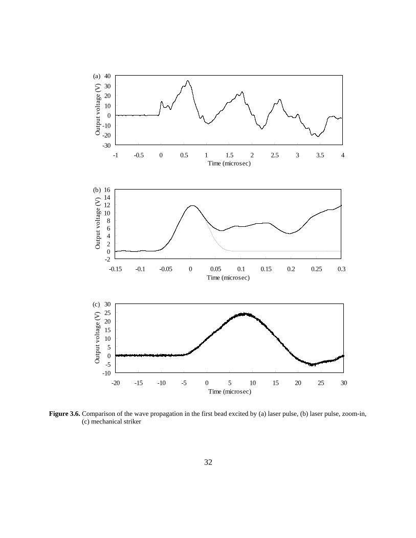
Figure 3.6. Comparison of the wave propagation in the first bead excited by (a) laser pulse, (b) laser pulse, zoom-in, (c) mechanical striker .............................................................. 32
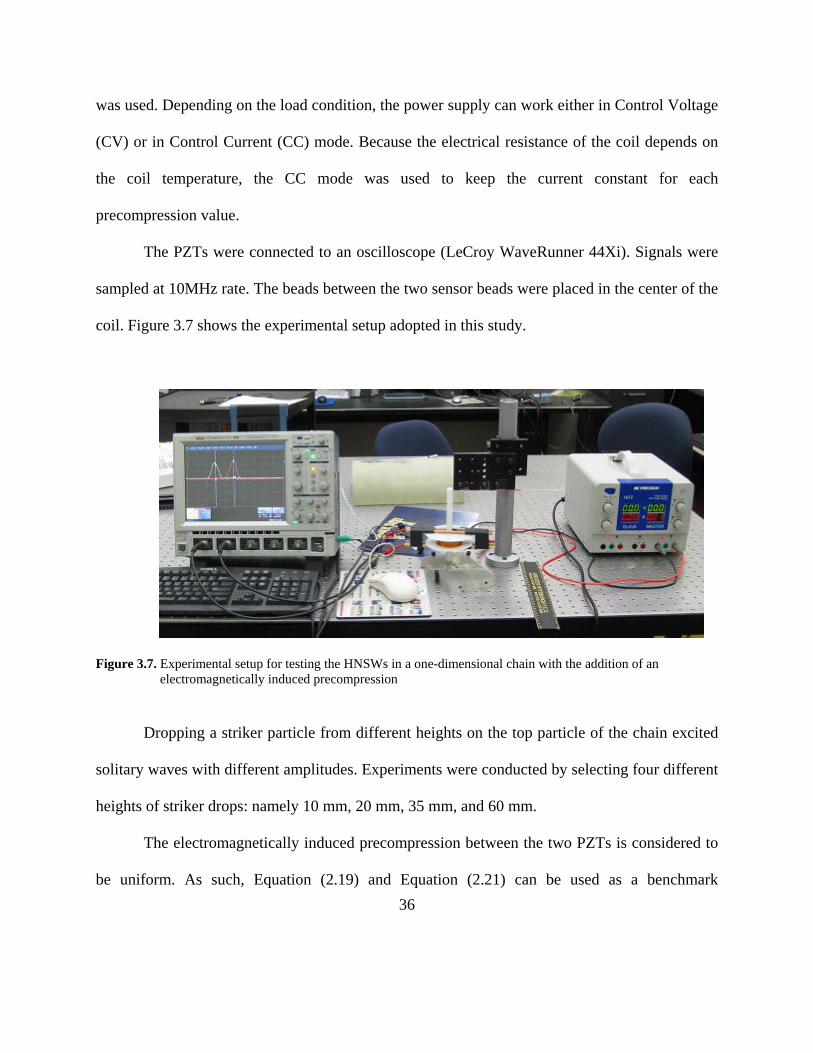
Figure 3.7. Experimental setup for testing the HNSWs in a one-dimensional chain with the addition of an electromagnetically induced precompression ..................................... 36
Figure 3.8. Photo and schematic diagram of the setup for measuring the precompression induced by the electromagnet .................................................................................................. 37
Figure 3.9. Electromagnetically induced pre-compression force as a function of the applied current ........................................................................................................................ 38
Figure 3.10. Typical HNSWs pulses obtained in the experiment ................................................. 39
xii
Figure 3.11. Dependence of the velocity of HNSWs on the magnitude of the dynamic contact force for both gravitationally and electromagnetically precompressed chain (PF denotes precompression) ........................................................................................... 40
Figure 3.12. Relationship between the duration of solitary wave and the dynamic contact force 42
Figure 4.1. Photo and sketch of the HNSW transducer for the remote and automatic generation of HNSWs (dimensions are expressed in mm) .............................................................. 46
Figure 4.2. Typical waveforms generated by the HNSW actuator ............................................... 47
Figure 4.3. Values of the dynamic force measured by both sensor beads .................................... 48
Figure 4.4. Wave speed as a function of the dynamic contact force at precompression equal to 0.053 N ...................................................................................................................... 49
Figure 5.1. Photo of the experimental setup for cement setting monitoring test .......................... 59
Figure 5.2. The force profiles measured from the 11th bead at different cement ages.................. 60
Figure 5.3. FEM simulation of HNSW interaction with gypsum cement samples in various elastic condition (done by J. Yang, D. Kathri and C. Daraio) ................................... 61
Figure 5.4. TOF of the PSW and SSW as functions of cement age ............................................. 61
Figure 5.5. Numerical results showing time of flight and propagating speed of HNSWs (done by J. Yang, D. Kathri and C. Daraio) ............................................................................. 63
Figure 5.6. The speed of the incident solitary wave and PSW as functions of cement age .......... 63
Figure 5.7. Amplitude ratios of PSW and SSW as functions of cement age ................................ 64
Figure 5.8. Measurements of cement compressive strength as a function of the cement age superimposed to the TOF variation of the PSW as recorded by the 11th bead .......... 65
Figure 5.9. Measurements of cement compressive strength as a function of the cement age superimposed to the ARP as recorded by the 11th bead ............................................ 65
Figure 5.10. Young’s modulus of 50-mm cubic cement samples as a function of cement age .... 66
Figure 5.11. Time-of-flight as a function of the Young’s modulus of 50-mm cubic cement samples ...................................................................................................................... 67
Figure 5.12. Schematics of the HNSWs-based NDE approach for monitoring concerte curing .. 73
Figure 5.13. Photo of the experimental setup of concrete curing monitoring test ........................ 75
Figure 5.14. Force profile of the HNSWs waveforms recorded at different ages of concrete (The force profiles are measured from the 11th bead in the HNSW transducer) ............... 76
xiii
Figure 5.15. TOF of the PSW and SSW and penetration resistance as a function of time ........... 77
Figure 5.16. Experimentally measured speeds of incident HNSW and PSW .............................. 78
Figure 5.17. The speed ratio of the incident HNSW to PSW ....................................................... 79
Figure 5.18. Experimentally measured ARP and ARS ................................................................. 80
Figure 5.19. Experiment setup of the two ton epoxy curing monitoring test ............................... 83
Figure 5.20. Typical waveforms at 0 minute, 90 minutes, 180 minutes, and 360 minutes .......... 84
Figure 5.21. (a) TOF and (b) AR as functions of curing time ...................................................... 86
Figure 5.22. (a) Scheme of the tested aluminum lap joint with location and types of defects at the bondline. (b) Locations of the inspected points (A, B, and C) within each region ... 89
Figure 5.23. Typical waveforms obtained at zone 1 and zone 6 ................................................... 90
Figure 5.24. (a) average of TOF and (b) average of ARP for all data at 36 inspection points from 12 zones ..................................................................................................................... 91
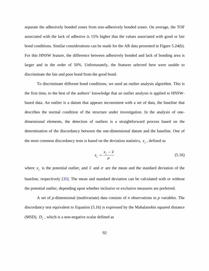
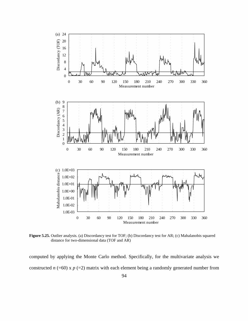
Figure 5.25. Outlier analysis. (a) Discordancy test for TOF; (b) Discordancy test for AR; (c) Mahalanobis squared distance for two-dimensional data (TOF and AR) ................. 94
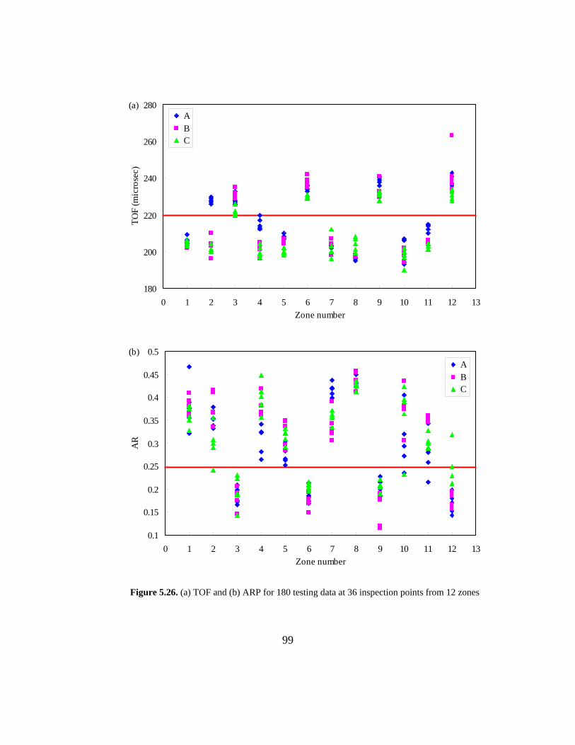
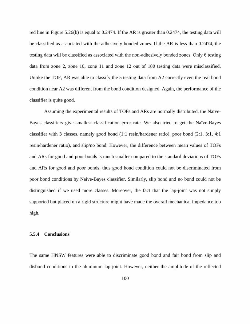
Figure 5.26. (a) TOF and (b) ARP for 180 testing data at 36 inspection points from 12 zones ... 99
Figure 5.27. Composite plate with impact damage. The centers are the test points 1-12 ........... 102
Figure 5.28. Photo of experimental setup for detecting impact damage in composite plate ...... 103
Figure 5.29. Typical waveform obtained from the pristine composite plate .............................. 103
Figure 5.30. HNSW features for test points on the composite plate. (a) TOF of PSW (b) TOF of SSW ......................................................................................................................... 104
Figure 5.31. HNSW features for test points on the composite plate. (a) ARP (b) ARS ............. 105
Figure 6.1. Schematic of the wave field in the linear medium shortly after the HNSWs impacts, color lines denote the wavefronts at different instants ............................................ 108
Figure 6.2. Distances from the chain made of certain material to the middle chain as functions of the dynamic contact force ........................................................................................ 112
Figure 6.3. Distances from the chain made of certain material to the middle chain as functions of the velocity of the strikers ........................................................................................ 113
xiv
PREFACE
First, I would like to thank Professor P. Rizzo for providing me the opportunity to perform this
research. I couldn’t finish this dissertation without his guidance and continuous support through
the process of my research.
I sincerely appreciate the collaboration with Dr. J. Yang, Dr. D. Kathri, Prof. C. Daraio at
Caltech, and Dr. S. Nassiri, Prof. J. Vandenbossche. I am thankful to Mr. C. Hager for his help in
preparing some of the experiments. The help from Mr. X. Zhu in Labview programming is
acknowledged.
Financial supports from NSF CMMI-0825983, 2009 ASNT Fellowship Award, and
MCSI are acknowledged.
Most of all, I owe my deepest gratitude to my wife and my mother for their love and
support.
1
1.0 INTRODUCTION
The rapidly expanding role of nondestructive evaluation (NDE), also usually called
nondestructive testing (NDT), in manufacturing, power, construction, and maintenance
industries, as well as in basic research and development, has generated a large demand for
practitioners, engineering, and scientists with knowledge of the subject [1]. NDE is defined by
the American Society of Nondestructive Testing (ASNT) as comprising those test methods used
to examine an object, material or system without impairing its future usefulness [2]. Properly-
employed NDE methods can have a dramatic effect on the cost and reliability of objects being
tested. The design of new engineering systems often incorporates novel materials whose long-
term degradation processes are not well understood. Existing infrastructures are aging and the
increase of axle loads on transportation grids is unavoidable. These circumstances demand that
damage in new or aging systems can be detected at the earliest possible time in an effort to
prevent life-threatening failures that can also lead to costly consequences for the taxpayers and
the environment. Effective NDE and Structural Health Monitoring (SHM) techniques able to
detect and quantify structural damage are therefore needed to ensure the performance, the proper
response, as well as the minimum maintenance costs of any engineering system.
2
This study attempts to develop a new NDE paradigm based on the use of highly nonlinear
solitary waves (HNSWs), able to detect defects at early stages and/or characterize the mechanical
properties of materials.
1.1 HIGHLY NONLINEAR SOLITARY WAVES
Highly nonlinear solitary waves (HNSWs) are mechanical waves that can form and travel in
highly nonlinear systems [3]. HNSW has a finite wavelength that is independent on its
amplitude. The wave speed and frequencyof HNSW are tunable. One-dimensional chain of
identical spheres is one of the most common systems that can support the generation and
propagation of HNSWs. HNSW in one-dimensional chain of spherical particles was first
investigated by Nesterenko [4] analytically and numerically and subsequently by Lazaridi and
Nesterenko [5] experimentally. The passage of HNSWs through the contact of two chains which
consist of spherical granules with different diameters and masses was investigated
experimentally and numerically by Nesterenko et al. [6]. Coste et al. [7] studied experimentally
the propagation of high-amplitude solitary waves in a chain of beads under Hertz contact,
subjected to a small static force controlled by a dynamometer. Falcon et al. [8] investigated the
collision of a one-dimensional column of beads with a fixed wall and developed a non-
dissipative numerical model based on a nonlinear interaction law between nearest neighbors
which gives results in agreement with the experimental data. Sen et al. [9] studied numerically
on the motion of an initial perturbation in a chain of spheres which are under Hertz contact. The
3
evidence of backscattering of the solitonlike pulse was presented in the presence of the light
mass impurities in the Hertzian chain. They suggested that the acoustic backscattering can be a
possible probe of buried light mass impurities in granular beds. Chatterjee [10] studied HNSWs
in an initially uncompressed one-dimensional chain of elastic spheres with power law interaction
where the power law index is greater than but close to unity. An asymptotic solution for the
solitary wave was developed. Sen et al. [11] conducted a numerical study on ejection of
ferrofluid gains using nonlinear acoustic impulses that might travel as nondispersive solitons.
The proposed mechanism has the potential to help design a nozzle-free inkjet printer of
unparalleled resolution. Coste and Gilles [12] demonstrated experimentally that at low static
precompression, for all beads made of different materials, the acoustic waves propagate in the
chain as predicted by Hertz’s theory. At larger precompression, after the onset of permanent
plastic deformation at the contacts, the brass beads exhibit non-Hertzian behavior. Hinch and
Saint-Jean [13] studied the fragmentation of a long line of stationary touching balls when hit on
its end by another ball for both linear contact law and Hertz contact law. Manciu et al. [14-15]
studied the propagation and backscattering of solution-like pulses in a chain of quartz beads with
Hertzian contacts. They presented preliminary data for three-dimensional granular beds and
suggested the soliton-like pulses can form and can be used as a valuable tool for probing buried
impurities in granular assemblies. Manciu et al. [16] presented a numerical study and
demonstrated that the crossing of identical solitary waves in a chain of discrete particles with
Hertzian contacts led to the spawning of weak secondary solitary waves at the point of
intersection of the solitary waves. Manciu et al. [17] studied the wave propagation in a chain of
elastic beads with dissipative contacts and randomly distributed masses. It was shown that even
4
in the presence of disorder, the impulse still travels as a compact object. Sen and Manciu [18]
obtained an iteratively exact solution to describe the solitary wave as a function of material
parameters and an infinite set of coefficients which depend on the power law index. Xu and
Hong [19] studied numerically the propagation, reflection and collision of solitary waves in the
vertical granular chain under gravity. Hong and Xu [20] found different characteristics in the
backscattered signal depending on the presence of light and heavy impurities in granular chain
and pointed out that the difference is due to soliton confinement in the region of the light
impurity of the granular chain. Manciu and Sen [21] expanded the study in [16] about the
formation of secondary solitary wave formation in systems with generalized Hertz interactions.
Nesterenko et al. [22] investigated the strongly nonlinear wave interaction with the interface of
two granular chains under magnetically induced precompression. Anomalous reflected
compression and transmitted rarefaction waves were observed. Job et al. [23] studied the
reflection of solitary waves in a chain of identical elastic beads at a wall with different elastic
properties numerically and experimentally. Vergara [24] studied numerically the scattering of
nonlinear solitary waves from an interface created by joining two one-dimensional chains of
spherical particles of different radii and masses. Dariao et al. [25] measured the propagation of
strongly nonlinear solitary waves in a chain of Teflon beads experimentally. The wave speeds
and profiles of solitary waves of the experimental results were in reasonable agreement with the
numerical solution based on the Hertz interaction law. Fast decomposition of long initial pulse
into a train of solitary waves and a speed of propagation of solitary wave well below the sound
speed in air were observed in the experiment. Hong [26] proposed that a granular container
having multiple interfaces with an appropriate alignment of elastic properties and masses may
5
play a role as an effective protector for an external impulse. Daraio et al. [27] investigated the
impulse confinement and the disintegration of the shock and solitary waves in one-dimensional
chains of alternating ensembles of beads with high and low elastic moduli and different masses.
It was found that the trapped energy is contained within the "softer" sections of the chain and is
slowly released in the form of weak and separated pulses over time. Daraio and Nesterenko [28]
experimentally measured the propagation of strongly nonlinear solitary waves in a chain of
polymer coated beads and showed that the chains of composite beads with a "hard" core and a
"soft" coating do support the Hertzian interaction and formation of strongly nonlinear solitary
waves. Daraio et al. [29] used a permanent magnet to apply static precompression to a chain of
Polytetrafluoroethylene (PTFE) or stainless steel beads to demonstrate the tenability of solitary
waves by adjusting the precompression. The experimental results agreed well with the long-wave
approximation and numerical calculations based on the Hertz contact law. Rosas et al. [30] had
explicitly demonstrated the two-wave structure in a granular chain without compression. Job et al.
[31] studied the solitary wave trains in granular chain analytically, numerically and
experimentally, and the results revealed that the amplitude of solitary waves decays
approximately exponentially along the chain. Porter et al. [32] investigated the propagation of
HNSWs in heterogeneous, periodic granular chains in which the stainless steel beads were
alternated with PTFE beads periodically. The experimental results are in good agreement with
the numerical simulation based on Hertzian interaction and the theoretical analysis of long-wave
approximation. Sen et al. [33] reviewed the studies on solitary waves in the granular chain,
introduced the theory of solitary waves in the chains of elastic beads, and discussed the possible
technological applications. Khatri et al. [34] studied the coupling between HNSWs in a one-
6
dimensional chain of beads and linear elastic media. The experimental observations agreed well
with the results from finite element analysis. Carretero-González et al. [35] proposed an
extended Hertzian model to account for the dissipative effect and developed optimization
methods to compute the exponents and prefactors in the extend model. The experiments on the
chains consisting of beads made of different materials revealed a common dissipation exponent
and a material-dependent prefactor. Porter et al. [36] expanded the work in [32] and extended the
existing theory from uniform granular lattices to non-uniform ones. Theocharis et al. [37]
investigated nonlinear localized modes in one-dimensional chains of compressed elastic beads
with one or two light-mass impurities. Molinari and Daraio [38] studied the existence of
stationary shock waves in uniform and non-uniform chains of spherical particles with Hertzian
contacts. Herbold et al. [39] investigated the formation and propagation of pulses in one-
dimensional chains of stainless steel cylinders alternated with PTFE spheres in linear, weakly
nonlinear and strongly nonlinear regimes. Fraternali et al. [40] applied the evolutionary
algorithm to study the optimal design of composite granular protectors using one-dimensional
chains of beads composed of various sizes, masses, and stiffnesses. Boechler et al. [41] used
experiments, theory, and numerical simulations to investigate the discrete breathers in a
compressed one-dimensional diatomic granular crystal. They analyzed how a modulational
instability generates discrete breathers in the weakly nonlinear regime and proved the existence
of discrete breathers experimentally. Theocharis et al. [42] further studied the existence and
stability of discrete breathers, and examined an unstable discrete gap breather centered on a
heavy particle with a symmetric spatial energy profile and a potentially stable discrete gap
breather centered on a light particle with an asymmetric spatial energy profile. Ponson et al. [43]
7
investigated the propagation of highly nonlinear waves in disordered granular chains composed
of diatomic units of spheres that interact via Hertzian contact. Each unit was oriented in one or
two possible ways, and the level of disorder in the chain is quantified by counting the number of
units with the same orientation. It was found that in low-disorder chains the solitary pulse
propagated with exponentially decayed amplitude and beyond a critical level of disorder the
wave amplitude decayed as a power law instead. Daraio et al. [44] investigated the propagation
of highly nonlinear pulses in a two-dimensional granular system that consists of a double Y-
shaped guide in which different mass/elastic modulus chains of spheres were arranged. The
numerical analysis agreed with the experimental results for most cases. Spadoni and Daraio [45]
introduced the generation and control of compact acoustic pulses (sound bullets) by a tuable,
nonlinear acoustic lens which consists of ordered arrays of granular chains. The amplitude, size
of sound bullets and the focusing location can be controlled by changing the static
precompression on the chains. The focusing effect was demonstrated by theory, numerical
simulation and experiment. Boechler et al. [46] presented an experiment to demonstrate that the
presence of a light-mass defect near a boundary in a statically compressed one-dimensional chain
of particles resulted in bifurcations and a subsequent jump to quasiperiodic and chaotic states.
The combination of frequency filtering effect and bifurcation could be used to achieve acoustic
switching and rectification. Leonard et al. [47] studied the wave propagation in a two-
dimensional square packing of uncompressed stainless steel beads excited by impulsive loadings.
The solitary waves only travelled through the initially excited chains. The results from the
experiment and numerical simulation were in good agreement. Boechler et al. [48] investigated
the tunable vibration filtering properties of a one-dimensional diatomic granular crystal
8
composed of periodic arrays of three-particle unit cells which were assembled with elastic beads
and cylinders that interact via Hertzian contact. The measured transfer functions of the crystals
using state-space analysis and experiments were in good agreement with the theoretical
dispersion relation analysis. Ngo et al. [49] studied the propagation of HNSWs in a one-
dimensional chain of ellipsoidal particles. The experimental results of the propagation properties
were found in good agreement with the theoretical prediction by long wavelength approximation,
the numerical simulation with discrete particle model, and the finite element simulation. Spadoni
et al. [50] experimentally studied the dynamic response of a nonlinear phononic crystal
composed of alternating steel disks and PTFE rings under precompression. Finite element model
was used to confirm the existence of a significant band gap and to reveal that some wave modes
are insensitive to precompression. Yang et al. [51] studied the interaction of HNSWs propagating
in granular crystals with adjacent linear elastic media. The characteristics of the reflected
HNSWs such as time-of-flight, amplitude ratio were correlated to the mechanical properties and
geometry of the linear media. The experimental results agreed with theoretical analysis based on
the long wavelength approximation and numerical simulation based on discrete particle model.
1.2 MOTIVATION AND OBJECTIVE
The overall objective of this project is to develop a new NDE/ SHM paradigm based on the use
of HNSWs, able to detect defects at early stages and/or characterize the mechanical properties of
materials. On a fundamental level, the study aims at characterizing the coupling between a highly
9
nonlinear oscillator and linear structures. From a purely applied perspective, the project will be
devoted to the validation of the fundamental studies and to the assembling of a new family of
actuators and sensors, their proof-of-principle testing on fundamental NDE/SHM problems, and
numerical validation.
1.3 STRUCTURE OF THE DISSERTATION
This dissertation is organized as follows. The theoretical background about HNSWs is presented
in Chapter 2. The fundamental research, which includes the laser generation of HNSWs and
tuning the HNSW by electromagnetical precompression, carried out in this study is presented in
Chapter 3. The development of a remotely and automatically controlled HNSW-based transducer
is described in Chapter 4. Then, the applications of HNSW in NDE and SHM including curing
monitoring of cement, concrete, and two ton epoxy, assessment of bond condition of aluminum
lap-joints, and damage detection in composite plate are presented in Chapter 5. Chapter 6
presents the preliminary study on acoustic lenses consisting of granular materials. Finally,
Chapter 7 discusses some directions for future studies on applications of HNSWs.
10
2.0 BACKGROUND ON HIGHLY NONLINEAR SOLITARY WAVES
HNSWs are compact waves characterized by unique tunable dynamic properties. For a system
consisting of a chain of spherical particles, solitary pulses can be excited by impacting one side
of the chain with a particle identical (or of equal mass) to the particles composing the chain.
The theoretical prediction of stress wave propagation in a chain of identical elastic beads
is given by Nesterenko [3] and has been demonstrated through quantitative experiments [5,7].
One peculiar characteristic of HNSWs is that their spatial wavelength is fixed and independent of
their amplitude. In a chain of particles, the wavelength of the pulse is about five particle
diameters. The amplitude and frequency, as well as the number of pulses generated in the
nonlinear systems can be tuned, for example, by changing the diameter of the bead, adding static
precompression to the chain of beads, changing the impact velocity and/or changing the shape of
the beads.
11
2.1 HERTZ INTERACTION LAW
The interaction between two adjacent beads in one-dimensional chains is governed by Hertz law
which was demonstrated by theoretical and experimental studies in [3-5,7]. Thus, the Hertz
interaction law is first introduced.
Figure 2.1. Cross-section of two spheres in contact (a) uncompressed, (b) compressed. δ is the approach of two spheres’ centers
When two spheres are compressed together by a static force F, they are in contact at a
small region which is not a singular point on either surface. Figure 2.1 shows the cross-section of
the surfaces of two spheres near the contact region. According to the theory of elasticity [52], the
radius of the contact region r is
12
3/1
21
213/1
+
=RRRDRFr (2.1)
where
−+
−=
2
22
1
21 11
43
EED νν (2.2)
and 1R , 2R , 1E , 2E , and 1ν , 2ν are the radii, the Young’s moduli, and the Poisson’s ratios of
the two spheres.
During the compression of between tow beads, the stress is much greater in the vicinity
of the contact region than throughout the rest of the beads. The bulk of the beads act as almost
undeformable bodies whereas the material in the neighborhood of the contact region acts as a
nonlinear spring. The relation between the static force F exerted on the spheres and the distance
of approach of their center δ is governed by Hertz’s interaction law [52]:
2/32/1
21
211 δ
+
=RR
RRD
F (2.3)
And the potential energy (Hertz potential) V is
2/52/1
21
21
52 δ
+
=RR
RRD
V (2.4)
For a chain composed of identical beads, Equation (2.3) becomes
2/31δAF = (2.5)
The material dependant constant
13
)1(32
21 ν−=
REA (2.6)
where R is the radius of the beads in the chain, E and ν are the Young’s modulus and the
Poisson’s ratio of the material.
It should be pointed out that the Hertz law is formulated for static problems, in order to
use it for solving dynamic problems, the following conditions need to be satisfied. (1) the
maximum stress achieved in the vicinity of the contact must be less than the elastic limit; (2) the
sizes of the contact surface must be much smaller than the radii of curvature of each particle; (3)
the characteristic times of the problem τ are much longer than the oscillation period of the basic
shape for the elastic sphere T [3-4]:
1
5.2cRT ≈>>τ (2.7)
where 1c is the velocity of bulk wave in the material of the interacting bead.
2.2 LONG WAVELENGTH APPROXIMATION
In this section, part of long wavelength approximation theory developed by Nesterenko [3-4],
which is related to the studies in this dissertation, is reviewed and summarized.
Let consider a one-dimensional chain of N identical beads with radius R and mass m
(Figure 2.2). Taking the precompression into account, let us assume that the chain is subject to a
constant precompression force F0, which is applied to the chain’s both ends and securing the
14
initial approach between the centers of adjacent beads 0δ . As a result of Newton’s laws of
motion,
Figure 2.2. One-dimensional chain initially compressed by a static force F0, small circles are the initial positions of beads and small triangles are the beads’ positions after perturbation, Fm denotes dynamic contact force
12,)()( 2/310
2/310 −≤≤+−−+−= +− NiuuAuuAu iiiii δδ (2.8)
where iu denotes the displacement of ith particle from its equilibrium position in the initially
compressed chain. For convenience, the coefficient A1 in Equation (2.6) is normalized by the
mass of beads m to get the constant A in Equation (2.8), mAA /1= . For the beads at both ends,
when 1=i , 2/3110
2/30 )( uuAAu ii +−−= +δδ , when Ni = , 2/3
02/3
10 )( δδ AuuAu iii −+−= − .
15
When the chain is initially “strongly” compressed, the dynamic deformation is much
smaller than the initial deformation:
10
1 <<−−
δii uu
(2.9)
In the anharmonic approximation, Equation (2.8) can be written as follows:
12))(2()2( 111111
−≤≤−+−++−= +−−+−+
Niforuuuuuuuuu iiiiiiiii βα
(2.10)
where
2/10
2/10 8
3,23 −== δβδα AA (2.11)
In the long wavelength approximation (L > a = 2R, where a is the diameter of the beads
and L is a characteristic spatial wavelength of the wave), the following equation can be obtained
from Equation (2.10):
xxxxxxxxxtt uuucucu σγ −+= 020 2 (2.12)
in which,
0
20
2022/1
020 ,
6,6
δσγδ
RcRcRAc === (2.13)
All terms of the order
+
0
34
2
20
δu
La
La
Lc
and higher were omitted in deriving
Equation (2.12). The solution of Equation (2.12) satisfies the Korteweg-de Vries (KdV) equation
and it will not be discussed here because it is beyond the scope of this study. When the chain is
initially “weakly” compressed,
16
10
1 ≥−+
δii uu
(2.14)
only one equation corresponding to the long wavelength approximation can be obtained from
Equation (2.8) for the discrete chain. The Equation (2.8) can be replaced by Taylor series
expansions according to the small parameter a/L. The wave equation in this case is
−−
−−−+−= 2/3
32
2/1
22/1
22/12
)()(
64)(8)(
8)(
23
x
xx
x
xxxxxxxxxxxxxxtt u
uauuuauuauucu (2.15)
where
)1(2,0 2
2
νπρ −=>−
Ecux (2.16)
and ρ is the density of particle material. The wave equation can be written in divergent form:
( )[ ]x
xxxxxtt uuaucu
−−+−−= 4/54/12
2/32 )()(10
)( (2.17)
[ ]xx
xxttac
+= )(10
4/54/12
2/32 ξξξξ (2.18)
where the strains 0>−= xuξ .
The stationary solutions for Equations (2.17) and (2.18) are summarized as follows:
The speed of solitary wave is
17
2/12/5
3/2
6/1
22320
2
2/12/50
2/12/3
02/52/5
00
)523(154
)1(1
)1(4
9314.0
)523(154
1
523(52
−+
−
−
=
−+
−=
−+
−=
rrr
rrr
mmm
s
faFE
c
cV
ξξνρ
ξξξ
ξξξξξξ
(2.19)
where mξ is the maximum strain, 0ξ is the initial strain caused by precompression F0, Fm is the
maximum dynamic contact force, fr is the force ratio, 0/ FFf mr = . 0c is the sound speed in a
chain with precompression F0 and force ratio 1=rf :
6/10
3/1
22/34/1
0
2/1
0 )1(29314.0
23 F
aEcc
−
=
=
νρξ (2.20)
When 00 =F , called “sonic vacuum”, rf or rξ is infinite, Equation (2.19) reduces to
6/13/1
22/34/1
)1(26802.0
52
mms Fa
EcV
−
==νρ
ξ (2.21)
The concept “sonic vacuum” is used for strongly nonlinear systems without a linear part
in the force displacement relation between particles and this type of systems do not support the
propagation of classical sound waves without initial precompression. The strain in this case is:
= x
acVs
510cos
45 4
2
2
ξ (2.22)
The solitary wave in sonic vacuum can be approximated by one hump of cos4 function.
The finite wavelength of stationary solution of solitary wave is
18
aaL 510
5≈=
π (2.23)
19
3.0 FUNDAMENTAL RESEARCH ON HNSWS
In this chapter the results from some fundamental researches carried out in this study are
presented. In particular, the capability to generate HNSWs by means of laser pulses is
demonstrated for the first time. In addition, by devising an electromagnet we show the tunability
of HNSWs by varying static precompression in a chain of particles made of low-carbon steel
beads.
3.1 LASER-BASED EXCITATION OF HNSWS
Single HNSWs are commonly induced in one-dimensional granular crystals by mechanically
impacting the first bead of the chain with a striker having the same mass of the particles
composing the chain. In this study we experimentally investigated the use of short duration (~ 8
nanoseconds) laser pulses to induce HNSWs in a one-dimensional chain of stainless steel
spheres. We analyzed the formation and propagation properties of the solitary pulses using
sensors placed in selected particles of the chain. The results were compared with the theoretical
prediction obtained from the long wavelength approximation [3-4,25,29].
20
3.1.1 Mechanism of laser generation of HNSWs
Laser generation of ultrasound was first demonstrated by White [53], since then lasers were
widely used to generate ultrasound in solids, liquids, and gases [54-55]. In this study, the laser
pulse was used to generate HNSWs in a chain of stainless steel beads. The mechanism of the
laser generation of HNSWs in a chain of stainless steel beads is briefly described here. The
transfer of energy from a nanosecond optical pulse to a mechanical wave can occur by
thermoelastic transduction or by ablation, depending on the intensity of the laser pulses and the
surface properties of the illuminated targets. A thermoelastic stress is created when the laser
energy density is low, such that there is no material ablation or plasma formation on the surface
of the object. In this regime, shear mechanical stresses are generated by the thermal expansion
due to the sharp increase of the surface’s temperature. Laser ablation is generated when the
laser’s power density is high, or when the surface of the illuminated medium is covered with a
film of water or gel. In this case the rapid vaporization (ablation) of the film at the surface, or the
melting of a small portion of the medium’s surface, induces high reaction pressures that can be
considered similar to normal stress loading [56-59]. Picosecond light pulses have also been used
to generate very short stress waves in films of different materials via thermal expansion [60].
The use of pulsed-laser excitations to trigger the formation of HNSWs has practical
advantages such as non-contact coupling between the laser and the chain of particles. This non-
contact excitation could be useful in applications where a remote placement of equipment or a
complex geometrical arrangement of the chains is required (e.g. in NDE of materials), or for
triggering multiple solitary waves in parallel chains (e.g. to generate sound bullets [45]).
21
In our experiments, we rely on the ablation of a controlled amount of water deposited
with a syringe on the surface of the first bead to generate mechanical stresses in the chain of
particles. In order to estimate the amount of mechanical stress transferred from the laser to the
chain, we assume that the energy transfer occurs only though the ablation of the water droplet
deposited on the first particle of the chain, and we describe the energy transfer using the
equations that govern the ablation of water on a flat metallic surface [55]. The incident power
density I of the pulsed laser is given by:
tAE
I L
∆= (3.1)
where EL is the energy of the laser, ∆t is the pulse duration, and A is the area of the pulse. The
ablation of material from the surface produces a net stress in reaction against the sample [55], in
the direction of the chain’s axis. This stress can be calculated from the rate of change of
momentum, i.e:
20
2
)]([ TTCLI
vw
a
−+=ρ
σ (3.2)
In Equation (3.2), aI is the absorbed power density, wρ is the density of water, L is the
water’s latent heat of vaporization, C is the thermal capacity of water, Tv is the vaporization
temperature of water, and 0T is the ambient temperature (293 K) at which the experiment was
conducted. For a polished mild steel irradiated by a 1064 nm laser pulse, the reflectivity
coefficient R is equal to 0.63 [55], the absorbed power density is equal to:
22
)1( RII a −= (3.3)
The effective force F generated by ablating the water droplet on the metallic surface is
equal to:
AF ⋅= σ (3.4)
This force is analogous to the dynamic contact force generated by a striker impacting the
top particle of the chain. If we assume that the amplitude of the pulse energy is constant over its
8 ns duration, then mechanical impulse J transferred to the chain of particle is given by:
tFJ ∆⋅= (3.5)
Table 3.1. Parameters used to compute the net stress force generated by the ablation of a drop of water on the flat surface of polished mild steel.
Parameter Value Unit
EL 150 x 10-3 J
Pulse diameter 0.5 x 10⁻³ m
∆t 8 x 10⁻⁹ Sec
ρw 1000 Kg / m3
L 2260 x 103 J / kg
C 4200 J / kg K
Tv 373 K
23
The impulse J is equivalent to the impulse generated by a striker bead having same mass
of the particle chains and falling from an effective height heq. If we assume the values shown in
Table 3.1, the impulse of the laser is equivalent to a falling mass of 0.45 g from an effective
height heq= 21 mm. This estimate is in agreement with experimental measurements performed
on the same chain of particles excited by a mechanical striker released from different heights,
which will be described in Section 3.2. In the experiment in Section 3.2, it was found that the
average maximum dynamic contact force measured between the 7th and 12th sensor beads when
the striker was released from 20 mm was equal to 21.44 N. As it will be shown in the Subsection
3.1.3, in the present study the average maximum dynamic contact force measured between the 9th
and 14th sensor beads was equal 10.54 N when the laser pulse energy was 150 mJ. It is important
to mention that the estimate of the effective drop height does not take into account the presence
of losses and attenuation in the system, and it is assumed that the laser pulse intensity is constant
in time (a better approximation would be obtained considering a Gaussian-like pulse). In
addition, the diameter of the laser pulse plays an important role: for example, a 1 mm pulse
diameter yields a heq = 1.4 mm.
3.1.2 Experimental setup
In our experiments, one-dimensional granular crystals were assembled by aligning twenty
stainless steel balls (Mc-Master Carr - Multipurpose Stainless Steel, Type 302) inside a vertical
Teflon tube having inner diameter equal to 4.8 mm. The diameter of each sphere was equal to
4.76 mm and the mass was 0.45 g. Two piezo-gauges made from lead zirconate titanate (square
24
plates 0.27 mm thick and 2 mm side) with nickel-plated electrodes and custom micro-miniature
wiring were embedded inside two of the steel particles. The assembling and calibration of the
instrumented particles was similar to that described in [3,25,29], and the calibration procedures
Figure 3.1. Experiment setup of observation of HNSWs propagating in a chain of steel beads (Actuator) excited by the laser pulse
25
will be described in Appendix A. The sensor beads were positioned along the chain at the 9th and
14th position from the top, and connected to an oscilloscope. Signals were sampled at 10 MHz.
To compare the experimental results with the theoretical predictions, the forces measured by the
instrumented bead (Fm,e) were related to the dynamic contact forces (Fm) as described in [25].
A 10 Hz repetition rate Nd:YAG pulse laser operating at 1064 nm wavelength was used
to excite stress waves in the chain of particles. The laser beam output diameter was equal to 7
mm. Through conventional optics (a 45 degrees high energy Nd:YAG mirror and a plano-convex
(PCX) UV fused silica lens, 25.4 mm diameter, and 100 mm focal length), a ~1 mm diameter
beam, as measured using a laser alignment paper, was directed on the surface of the first particle
of the chain. The laser was operated in single-shot mode. To apply variable amounts of static
precompression on the chain of particles, we placed above the chain a polycarbonate sheet,
loaded with variable balanced masses. To allow direct interaction of the laser beam with the first
particle in the chain, a 3 mm diameter hole was drilled in the center of the sheet. The photo and
schematic diagram of the experimental setup are presented in Figure 3.1.
3.1.3 Results and discussion
We investigated the effects of the beam intensity and of the precompression on the
characteristics of the solitary waves. To determine the effects of the energy we varied the laser’s
energy output between 120 mJ and 190 mJ with 10 mJ increments. As the diameter of the beam
impinging the top particle of the chain was equal to 1 mm the energies can be straightforwardly
related to the laser intensities expressed in 15.28 J/cm2 to 24.17 J/cm2 with 1.27 J/cm2
26
(a)
-1012345678
0 25 50 75 100 125 150 175 200Time (microsec)
Dyn
amic
forc
e (N
) 9th bead 14th bead Theory
(b)
-3-2-10123456
0 25 50 75 100 125 150 175 200Time (microsec)
Dyn
amic
forc
e (N
) 9th bead 14th bead Theory
(c)
-3-2-1012345
0 25 50 75 100 125 150 175 200Time (microsec)
Dyn
amic
forc
e (N
) 9th bead 14th bead Theory
(d)
-4-3-2-1012345
0 25 50 75 100 125 150 175 200Time (microsec)
Dyn
amic
forc
e (N
) 9th bead 14th bead Theory
Figure 3.2. Comparison of the pulse shape obtained in experiments with a theoretical cos4 function
27
increments. To study the effect of precompression, we used four different values of
precompressive force: 0.049 N, 2.305 N, 3.384 N, and 5.150 N. These static preloads were
applied placing balanced masses on the polycarbonate sheet. The values include the self-weight
of the top eleven beads.
Typical time waveforms recorded by the two instrumented particles in the chain at four
different values of precompression and 160 mJ laser energy (equivalent to an energy density of
20.37 J/cm2) are shown in Figure 3.2. For comparison, a cos4 function (Equation. (2.22)) [3] was
superimposed to the measured waveforms. As expected, at low values of precompressive force
(Figure 3.2(a)) the shape of the experimental pulse is in excellent agreement with predictions
from the highly nonlinear theory. However, with increasing amount of precompression with
respect to the amplitude of the dynamic force Fm,e, the response of the chain shifts from the
highly nonlinear regime towards the weakly nonlinear and linear response. This is evident from
the appearance of an increasingly large tensile part of the pulse in Figure 3.2(b,c,d) and from the
presence of additional oscillations following the leading pulse.
The speed of the HNSW was calculated by detecting the arrival time of the pulse's peak
in the instrumented beads and knowing their relative distance in the chain. We compared this
speed with the amplitude of the traveling pulses. Figure 3.3 shows the HNSW’s speed as a
function of the dynamic contact force. The experimental values are shown by solid dots and the
theoretical curves are represented by solid lines. In Figure 3.3(a), the vertical error bars are the
results of possible inaccuracy on the estimation of the peak’s arrival time and on the
measurement of the travel distance between the two piezosensors. In Figure 3.3(b), the horizontal
error bars are the results of accuracy of the sensors’ calibration coefficients. To ensure
PF = 0.04 N (Experimental) PF = 0.75 N (Experimental) PF = 1.64 N (Experimental) PF = 0.04 N (Theoretical) PF = 0.75 N (Theoretical) PF = 1.64 N (Theoretical)
Figure 3.11. Dependence of the velocity of HNSWs on the magnitude of the dynamic contact force for both gravitationally and electromagnetically precompressed chain (PF denotes precompression)
Equation (2.19) reveals that the speed Vs of a HNSW depends on the pre-compressive
force F0. Figure 3.11 shows the theoretical prediction of the wave speed when the pre-
compressive force (PF) is equal to 0.04 N, 0.75 N, and 1.64 N. Experimental data obtained in
this study is overlapped to the theoretical predictions. For each measurement, the maximum
value of the dynamic force Fm,e, measured by the embedded PZT, was converted to the
41
maximum contact force between neighboring beads Fm using Equation (3.7). The coefficient β
was obtained from Figure 2 of reference [29].
The relationship between the velocity of the solitary wave and the applied current was
investigated for the four different heights from which the striker was released. For each height
and applied precompression, 10 acquisitions were obtained.
Even the striker was released from the same height, the dynamic force amplitude changes
as the applied current changes. Such behavior is expected since there exists a change in the
current/magnetic field results in a change of the striker’s velocity as it approaches the top bead
due to the magnetic force between the striker and the chain of beads. Furthermore, the coefficient
β in Equation (3.7) also changes as the ratio of Fm,e/F0 changes. Taking this into consideration,
theoretical wave speeds for all acquisitions were calculated.
Table 3.2. The maximum and average errors of wave speeds
Height (mm) Maximum error (%) Average error (%)
I=0A I=1A I=2A I=0A I=1A I=2A
10 3.02 2.19 3.70 1.48 1.07 1.99
20 3.77 3.62 2.98 1.80 1.26 1.81
35 2.55 2.18 1.53 1.36 1.08 0.82
60 3.46 2.95 5.07 1.56 0.87 2.47
42
The maximum and average errors for each height and current are listed in Table 3.2. The
good agreement between the theoretical prediction and the experimental results is visible.
Because the solitary waves observed in the experiments may have tails [7,25,29], it is difficult to
decide where the beginning and end of each pulse are. Instead, the time interval, t, between
instants in which the pulse reaches half of its amplitude for the first time and the crest, is
considered. From the geometry of the solitary wave, theoretically A*cos4(ωt), the duration of the
solitary wave, T, can be calculated as:
ttT 49.5)2(sin2
24/11 ≈
−= −−π
π (3.8)
25
30
35
40
45
50
10 15 20 25 30 35 40 45
Dynamic contact force (N)
Dur
atio
n of
HN
SWs (
mic
rose
c)
PF = 0.04 N PF = 0.75 N PF = 1.64 N
Figure 3.12. Relationship between the duration of solitary wave and the dynamic contact force
43
The relationship between the duration of the solitary wave, T, and the dynamic force
magnitude, Fm, is shown in Figure 3.12. It can be seen that the duration of the pulse increases as
the dynamic force magnitude decreases. This implies that the increase of the dynamic contact
force increases the frequency of the HNSWs. When the dynamic contact force stays constant, the
pre-compression has little effect on the duration/frequency of the solitary pulse; however, the
pre-compression force applied in this experiment is relatively small.
The products of wave speeds Vs and durations T, which are equal to the wavelength of
the HNSWs, were calculated and the results are shown in Table 3.3. The products which
represent the spatial wavelengths are expected to be equal to five bead diameters, i.e. long, 23.8
mm in this case.
Table 3.3. The products of wave speeds and durations
Height (mm)
Average of product of wave
speed and duration (mm) Relative standard deviation (%)
I=0A I=1A I=2A I=0A I=1A I=2A
10 23.0 26.3 25.4 4.07 3.70 6.83
20 23.1 23.9 26.1 7.08 5.57 5.15
35 23.1 24.2 25.8 9.65 7.98 4.54
60 22.7 23.3 22.2 5.11 5.44 8.48
44
3.2.4 Conclusions
In this section an electromagnetically induced precompression was applied to a one-dimensional
chain of 20 general purpose low-carbon steel beads. The ability of using an electromagnet to tune
solitary waves propagating in the chain of ferromagnetic beads is demonstrated experimentally.
The wave speed, amplitude and duration were measured for three different electric
currents and four different heights from which the striker was released. These tests vary the value
of the static precompression applied to the chain and the dynamic contact force. The
experimental results agree very well with the theory derived from the long wavelength
approximation.
The following conclusions can be drawn: (1) A wire wound into a coil can generate an
electromagnetic field that can be used to apply a variable static precompression to a chain of
general purpose low-carbon steel beads; (2) When the precompression is constant, the wave
speed increases as the dynamic contact force increases. When the dynamic contact force is
constant, the wave speeds increases as the precompression increases. This concept was
demonstrated experimentally by using an electromagnet to adjust precompression and by
changing the height from which the striker was released, thereby changing the velocity of the
striker; (3) The product of wave speed and duration witnessed little change, indicating very little
change in the spatial wavelength, as well.
The method presented in this section provides an easy way to tune the HNSWs
propagating in a one-dimensional chain of ferromagnetic or weakly magnetic beads.
45
4.0 DESIGN OF A HNSW TRANSDUCER
This chapter introducers a HNSW-based transducer (hereafter referred as HNSW transducer)
designed and built during this study. The effectiveness of the HNSW transducer to generate
repeatable solitary waves was demonstrated through a simple experiment.
4.1 DESCRIPTION OF THE HNSW TRANSDUCER
A novel actuator was designed for the remote and automatic generation of HNSWs. Figure 4.1
shows a photo and the schematic of the HNSW transducer developed in this study. It consisted of
a 4.8 mm diameter PTFE tube containing twenty stainless steel beads. Each bead was 4.76 mm
in diameter and 0.45 g in weight. A low-carbon steel bead which has the same mass equal to 0.45
g was used as a striker. The pipe was surmounted by an electromagnet consisting of a coil of an
AWG24 magnetic wire wrapped around an iron core. The iron core was a 13 mm diameter and
33 mm long rod. The electric resistance of the coil was equal to 7.4 Ω. The electromagnet was
collocated inside a PTFE pipe with internal diameter equal to 39 mm, designed to accommodate
also the tube containing the chain of particles. Once activated, the electromagnet was able to lift
the striker up to 10 mm. For this actuator, the particles used to assemble the chain were made of
46
a non-ferromagnetic material to avoid undesired interactions between the beads in the chain and
the electromagnet.
Figure 4.1. Photo and sketch of the HNSW transducer for the remote and automatic generation of HNSWs (dimensions are expressed in mm)
In order to further increase the range of impact velocities achievable with this actuator
design, the direct current flowing in the electromagnet can be increased or the design of the coil
can be modified by increasing the number of turns per unit length.
4.2 VALIDATION OF THE HNSW TRANSDUCER
To evaluate the capability of the transducer to generate HNSWs, the chain was instrumented
with two sensors beads, positioned along the chain at the 10th and 15th position from the top and
47
connected to an oscilloscope. For this experiment the falling distance of the striker was set equal
to 8.5 mm. In order to assess the repeatability of the generated pulses, fifty measurements were
taken.
Typical force profiles generated by the HNSW transducer and recorded by the sensor
beads are presented in Figure 4.2, where the experimental time histories are overlapped to a cos4
function, which represents the shape of the pulse predicted by the long wavelength analysis [3].
The agreement between the experimental and the ideal pulses is evident.
-2
0
2
4
6
8
10
12
0 25 50 75 100 125 150 175 200 225Time (microsec)
Dyn
amic
forc
e (N
)
10th Experimental
15th Experimental
Theoretical
Figure 4.2. Typical waveforms generated by the HNSW actuator
Figure 4.3 shows the maximum dynamic force obtained in all fifty measurements
extracted from the 10th and 15th bead. The mean value of the dynamic force measured at the 10th
particle was equal to 11.51 N with a standard deviation equal to 0.34 N, which is only 2.98% of
48
the mean value. The average value recorded by the 15th particle was equal to 11.38 ± 0.36 N. In
this case, the standard deviation was equal to 3.17% of the mean value. The small standard
deviations indicate the high repeatability of the signal generated with this transducer. It should be
noted that the average dynamic force measured by the top sensor bead is only 1.17% greater than
that measured by the bottom sensor bead. This indicates that the pulse’s attenuation in the
actuator was very small.
9
9.5
10
10.5
11
11.5
12
12.5
13
0 5 10 15 20 25 30 35 40 45 50Measurement number
Dyn
amic
forc
e (N
)
Top Bottom Top average Bottom average
Figure 4.3. Values of the dynamic force measured by both sensor beads
The speed of the HNSW was calculated by detecting the arrival time of the pulse's peak
in the instrumented beads and knowing their relative distance in the chain. Figure 4.4 shows the
experimentally calculated wave speed as a function of the dynamic contact force. The theoretical
prediction obtained from the long wave approximation is overlapped. The agreement between
49
experimental data and theoretical prediction is very good and it confirms the ability of the
actuator to generate HNSWs.
450
500
550
600
650
14 15 16 17 18Dynamic contact force (N)
Wav
e sp
eed
(m/s
)
ExperimentalTheoretical
Figure 4.4. Wave speed as a function of the dynamic contact force at precompression equal to 0.053 N
The designed HNSW transducer is compact, low cost and easy-to-control. It has good
repeatability, tunability and doesn't need couplant and the use of electrical arbitrary function
generator. The actuator consists of a one-dimensional chain of particles surmounted by an
electromagnet that lifts and releases the striker from a certain height. By remotely activating the
electromagnet the movement of the striker can be guaranteed with high level of repeatability.
This automatic excitation of HNSWs could be useful in applications where a remote placement
of equipment or a complex geometrical arrangement of the chains is required. This design also
allows increasing the repetition rate of the generated pulses which, in turn, can be useful in certain
50
applications such as nondestructive testing. Two piezo-gauges made from lead zirconate titanate
with nickel-plated electrodes and custom micro-miniature wiring were embedded inside two of
the steel particles to measure the incident and reflected HNSWs.
51
5.0 APPLICATIONS OF HNSW-BASED METHODS FOR NDE
In this chapter the applications of HNSW-based methods in the area of NDE and SHM are
presented. The first section of this chapter illustrates general principle of the HNSW-based
methods. Then, the rest of this chapter presents curing monitoring of cement, concrete, and two
ton epoxy, assessment of bond condition of aluminum lap-joints, damage detection in composite
plate by HNSW-based methods.
5.1 GENERAL PRINCIPLES OF HNSW-BASED METHODS FOR NDE
The interaction between HNSWs and linear materials at the interface between a chain of particles
and a bulk material has been investigated by few researchers [8,19,23]. Falcon et al. [8] studied
the bouncing behaviors of the impact at the interface between a chain of beads and a fixed wall.
The solitary wave reflection at a rigid wall boundary has been studied by Xu and Hong [19]. Job
et al. [23] investigated the collision of a single solitary wave with elastic walls with different
hardness. The interaction of HNSWs with linear elastic media and the formation and propagation
of reflected solitary waves were studied both theoretically, numerically and experimentally [51].
It shows that the formation and propagation of reflected solitary waves are highly dependent on
52
the elastic modulus and geometry of the adjacent linear medium. Furthermore, the observed
sensitivity of reflected solitary waves to elastic modulus and geometry of both the adjacent
materials and underlying layers, and it is important for monitoring the hydration process of
cementitious materials because the specimen can't afford the weight of the actuator at the early
stage of curing without putting an additional layer to enlarge the area of the interface.
In general, it has been observed that when the incident wave interacts with a "soft"
neighboring media the formation of a primary reflected solitary wave (PSW) and a secondary
reflected solitary wave (SSW) are formed. The transit time at a sensor particle between the
incident and the reflected waves are referred as time-of-flight (TOF). The ratio of the PSW’s
amplitude to the amplitude of the incident solitary wave is referred as amplitude ratio of primary
reflected solitary wave (ARP) and the ratio of the SSW’s amplitude to the amplitude of the
incident solitary wave is referred as amplitude ratio of secondary reflected solitary wave (ARS).
The interaction with the "soft" interface results in a delayed formation of the PSW and SSW.
Here, the theoretical analysis by Yang et al. [51] is reviewed. For a chain of elastic beads
interacts with a semi-infinite wall, assuming the kinetic energy of the striker is split between the
Hertzian potential and the kinetic energy of the last bead against the bouncing wall, the contact
time between last bead and the wall can be estimated as:
5/25/15/2218.3 −−≈wkc AVmT (5.1)
where kV is the velocity of the striker, and the bead-wall contact stiffness w
A is given as:
53
122 113
4−
−+
−=
w
ww EE
RAνν (5.2)
where wE and wν are the Young’s modulus and Poisson’s ratio of the wall material.
122 113
4−
−+
−=
w
ww EE
RAνν (5.3)
From the Nesterenko’s long wavelength approximation [3-4], the speed of the incident
solitary wave iV is given as:
5/1
2
25/1
)2(2516
=
mAv
RV cii (5.4)
where iv is the bead incident velocity which was found ki Vv 682.0≈ by Chatterjee [10], and the
bead-bead contact stiffness c
A is given as:
)1(32
2ν−=
REAc
(5.5)
Assuming the difference between the speed of the incident solitary wave and that of the
reflected solitary wave can be ignored, the traveling time of solitary wave in the chain is
it V
RNT 14= (5.6)
where 1N is the number of beads between the sensor bead and the wall.
54
Replacing bV in Equation (5.4) and substituting Equation (5.4) into Equation (5.6), we
get the traveling time of in the chain
5/25/15/21361.2 −−≈
ckt AVmNT (5.7)
The TOF and PSW can be expressed as
5/125/2
15/2 )361.2218.3(
+≈+= −−
kcwtcPSW V
mANATTTOF (5.8)
When the chain is in contact with two-layer composite media, based on the momentum
and energy conservation, the ratio of the last bead reflection velocity rv to the incident velocity
iv can be approximated as:
u
u
i
r
MmMm
vv
+−
= (5.9)
where uM is the mass of the layer which is in direct contact with the chain.
Based on Equation (5.4),
5/1
=
i
r
i
r
vv
VV
(5.1
0)
where rV is the speed of the reflected solitary wave. Then the traveling time tT ′ in this case is
+=′
rit VV
RNT 112 1 (5.11)
Substituting Equations (5.6) and (5.10) into Equation (5.11), we can get
55
+−
+=′− 5/1
12 u
utt Mm
MmTT (5.12)
The TOF of PSW for the chain in contact with two-layer composite is
5/125/15/2
15/2 1181.1218.3
+−
++≈
′+=−
−−
ku
ucw
tcPSW
Vm
MmMm
ANA
TTTOF
(5.13)
The contact delay lT between two layers of composite is
d
ul k
MT π= (5.14)
where dk is the stiffness of the second layer of the composite.
Then, the TOF of PSW can be expressed as the sum of the TOF of PSW and the linear
medium contact delay:
d
u
ku
ucw
lPSWSSW
kM
Vm
MmMm
ANA
TTOFTOF
π+
+−
++≈
+=−
−−5/125/1
5/21
5/2 1181.1218.3 (5.15)
To estimate the ARP and ARS or to get more accurate estimation of TOFs, numerical
simulation or finite element analysis can be used and the dissipation and restitution loss need to
be considered in these models.
56
5.2 SETTING MONITORING OF PLASTER OF PARIS BY HNSW
In this section we present a nondestructive technique based on the propagation of HNSWs to
monitor the hydration of cement. The HNSW transducer was used to inject HNSWs into a
sample of fresh gypsum cement and to detect the waves reflected from the cement’s surface. We
assessed the hydration process of the cement specimen by analyzing the time-of-flight and the
amplitude of the reflected HNSWs. We found that the wave’s properties were dependent on the
mechanical properties of the cement paste. We compared the experimental results with numerical
simulations (done by colleagues J. Yang, D. Kathri and C. Daraio from Caltech) based on a
simplified finite element model, and compared the Young’s modulus and ultimate compressive
strength obtained nondestructively with the same quantities obtained from destructive tests. We
observed good agreement between experiments and numerical simulations for all cases
considered.
5.2.1 Introduction
The quality and the durability of cement-based products are influenced by early stages of
hydration [62-63]. The observation of the hydration process in cement-based materials permits to
predict their long-term behavior, and to accurately estimate their setting time [64-65]. In the past
20 years, several NDE techniques have been proposed to monitor the hydration of cement. These
methods correlate certain mechanical, electrical, or acoustical parameters with the cement or
concrete properties by using empirical relationships [66]. The most widely used NDE technique
57
is based on the propagation of ultrasounds [64-65,67-80]. Other methodologies make use of
electromagnetic waves [81-82], electrical resistivity [79], and X-ray diffraction [75]. In
ultrasonic-based methods, cement samples are typically inspected by commercial transducers
that generate longitudinal [65,68-71,75-77,79-80] or longitudinal and shear [64,72-73] bulk
waves. Parameters such as wave speed and attenuation are then measured and empirically
correlated to the cement material properties. This approach is usually referred to as the ultrasonic
pulse velocity (UPV) method [83]. To obtain good signal-to-noise ratio, longitudinal wave
transducers cannot be used to generate transverse waves and vice versa. Thus, to use both shear
and longitudinal waves, at least four transducers are necessary. If the access to the back wall of
the sample is not practical, the wave reflection method can be adopted. In this approach, the
reflection loss of ultrasonic shear [67,74] or longitudinal [65,77,82] waves at an interface
between a buffer material, typically a steel plate, and the cementitious material is monitored over
time. The amount of wave attenuation depends on the reflection coefficient, which in turn is a
function of the acoustical properties of the materials that form the interface [66].
In this section, we propose a novel NDE paradigm to monitor cement hydration at early
age based on the use of HNSWs. The HNSW transducer described in Chapter 4 was used. We
injected a single pulse of HNSW into a cement specimen using a granular crystal and propose to
monitor the hydration process by measuring the reflected waves formed at the actuator/cement
interface.
The experimental results are compared to a simplified finite element model (using
ABAQUS), and to the ultimate compressive strength and Young’s modulus of cement cubes
obtained following the ASTM C109 [84]. The experimental results from the proposed HNSW-
58
based method are in good agreement with numerical data, and they show strong correlation with
the measured mechanical properties obtained from destructive tests of the cement specimens.
With respect to previous works, the novelty and the advantage of this HNSW-based NDE
technique is multifold: 1) it exploits the propagation of HNSWs in granular systems; 2) it
employs a cost-effective actuator/sensor in a combined form; 3) it measures several waves’
parameters that can be used to correlate multiple cement variables; 4) it does not require, unlike
UPV method, the exact knowledge of the distance between a transmitter and a receiver and does
not require the access to the sample back-wall.
5.2.2 Experimental setup
To evaluate the proposed NDE methodology, we prepared one conical frustum sample of fast
setting USG® Ultracal 30 gypsum cement. This material is low expansion rapid-setting gypsum
cement used in the building industry as a surface finish of interior walls and in the production of
drywall products for interior lining and partitioning. In our experiment we prepared a paste with
water and cement in a ratio of 0.38 in weight, as recommended by the manufacturer. The paste
was poured into a plastic mold after 5 minutes of mixing. The conical frustum sample obtained
from the mold was 77 mm high, with top and bottom diameters equal to 62 mm and 42 mm,
respectively. A 40 × 40 × 0.254 mm aluminum sheet was placed on top of the specimen 30
minutes after pouring the paste in the mold, and the granular chain actuator was placed on top of
the sheet 7 minutes later. The experimental setup is shown in Figure 5.1. A DC power supply
provided current to activate the electromagnet located on the top of the granular chain.
59
Instrumented sensor particles inserted in the 11th and 16th particle positions measured the incident
and reflected HNSWs, which were recorded by an oscilloscope. The signals were digitized at 5
MHz sampling rate. Five measurements were taken every three minutes during the first 90
minutes of the cement age. Then, five measurements were recorded every six minutes until
cement age was 180 minutes. Monitoring was stopped three hours after mixing, in accordance to
the manufacturer’s nominal setting time.
Figure 5.1. Photo of the experimental setup for cement setting monitoring test
60
5.2.3 Experimental results
5.2.3.1 HNSW measurements
Figure 5.2 shows the time history of the force measured by the 11th particle in the chain, at five
different times of the hydration process. The top plot represents the HNSW profile after 45
minutes of curing process, while the bottom plot shows the force signal measured after 120
minutes of cement age. In this figure, the incident pulse and the primary and secondary reflected
waves are clearly visible. We also observe that the shape, amplitude, and travel time of the
reflected waves changed with time. It is notable that Figure 5.2 is very similar to Figure 5.3,
implying a close relationship between cement’s curing time and its elastic modulus. The
variation of elastic modulus as a function of the curing time will be addressed in subsection
5.2.3.3.
Figure 5.2. The force profiles measured from the 11th bead at different cement ages
61
Figure 5.3. FEM simulation of HNSW interaction with gypsum cement samples in various elastic condition (done by J. Yang, D. Kathri and C. Daraio)
100
200
300
400
500
600
700
45 60 75 90 105 120 135 150 165 180Time (min)
TOF
(mic
rose
c)
SSW PSW
Figure 5.4. TOF of the PSW and SSW as functions of cement age
62
Figure 5.4 shows the measured TOFs of both primary (blue line with circles) and
secondary (red line with squares) reflected waves as a function of the hydration time. Each dot
indicates the mean value of the five experimental measurements, and the vertical error bars
represent the 95.5% (2σ) confidence interval. The barely visible error bars demonstrate the
repeatability of the proposed methodology. The trend evident in Figure 5.4 clearly denotes the
presence of a two-stage evolution. In the first stage, lasting between 45 and 90 minutes, the TOF
values of PSW and SSW decrease approximately exponentially. After 90 minutes the variation of
the TOF plateaus, changing only slightly with increasing cement age. The trends observed in
these results are well captured by the numerical data in Figure 5.5. Discrepancies between
numerical data and Figure 5.4 stem from the different physical parameters used in the horizontal
axis and from the approximations used in the numerical model. Figure 5.6 shows the wave speed
of the incident solitary wave (blue line with circles) and of PSW (red line with squares) as a
function of curing time. Similarly to the analysis of the TOF, we find that the speed of the
primary reflected waves becomes less sensitive to the materials properties of the cement, as the
curing time progresses. We also observe that the incident wave velocity remains almost constant
in all tests performed.
The variations of the ARP and the ARS as a function of the cement age are shown in Fig.
10. While the amplitude ratio of the primary wave shows increases with cement age (blue line
with circles), the ARS exhibits a relatively complex behavior during the curing process (square
red line). It is worth noting that the amplitude of the primary reflected wave has a six-fold
increase with respect to the fresh cement.
63
Figure 5.5. Numerical results showing time of flight and propagating speed of HNSWs (done by J. Yang, D. Kathri and C. Daraio)
320
360
400
440
480
520
560
600
45 60 75 90 105 120 135 150 165 180Time (min)
Wav
e sp
eed
(m/s
)
incident solitary wavePSW
Figure 5.6. The speed of the incident solitary wave and PSW as functions of cement age
64
0
0.1
0.2
0.3
0.4
0.5
0.6
0.7
45 60 75 90 105 120 135 150 165 180
Time (min)
Am
plitu
de ra
tio
PSW SSW
Figure 5.7. Amplitude ratios of PSW and SSW as functions of cement age
5.2.3.2 Compressive strength test
Uniaxial compression tests were performed according to ASTM C109 [84] using a Test Mark
machine operated in displacement control. Eighteen 50-mm cubes were prepared using the
water-to-cement ratio (0.38 in weight) suggested by the manufacturer. The paste mixture was
blended three minutes prior to pouring into the molds. Each sample was removed from the mold
before testing. Figure 5.8 shows the measured compressive strength as a function of the
hydration time superimposed to the TOF variation of the PSW as recorded by the 11th bead. We
observe that the cement strength increases drastically up to the cement age of 90 minutes and
becomes approximately identical afterwards. This is in agreement with the behavior of extracted
features from HNSWs, as observed in Figure 5.4.
65
0
4
8
12
16
20
24
60 75 90 105 120 135 150 165 180Time (min)
Com
pres
sive
stre
ngth
(MPa
)
0
20
40
60
80
100
120
140
160
180
200
TOF
varia
tion
(mic
rose
c)
StrengthHNSW-based feature
Figure 5.8. Measurements of cement compressive strength as a function of the cement age superimposed to the TOF variation of the PSW as recorded by the 11th bead
0
4
8
12
16
20
24
60 75 90 105 120 135 150 165 180Time (min)
Com
pres
sive
stre
ngth
(MPa
)
0.26
0.31
0.36
0.41
0.46
0.51
0.56
0.61
AR
P
StrengthHNSW-based feature
Figure 5.9. Measurements of cement compressive strength as a function of the cement age superimposed to the ARP as recorded by the 11th bead
66
To compare the measured strength with the HNSW responses, we superimpose the plots
of TOF and ARP on the top of the strength curve as shown in Figure 5.8 and Figure 5.9
respectively. For the sake of comparison, we used “TOF variation” in Figure 5.8, which
represent the deviation of the measured TOF values from the TOF recorded at 65 minutes. As
demonstrated in both Figure 5.8 and Figure 5.9, the behavior reflected HNSWs match well with
the measured strength of cement specimens. This implies the ability of the novel HNSW-based
NDE approach to capture the variation of the cement’s compressive strength.
5.2.3.3 Young’s modulus test
0
0.5
1
1.5
2
2.5
3
3.5
4
4.5
5
60 75 90 105 120 135 150 165 180Time (mins)
You
ng's
mod
ulus
(GPa
)
Experimental results A fitted curve
Figure 5.10. Young’s modulus of 50-mm cubic cement samples as a function of cement age
To measure the elastic modulus of the cement paste, ten 50-mm cubes were tested with a load
frame (MTS Systems Corporation, frame number 810, load cell number 661.21) operated in
67
displacement control. Both compressive force and displacement were recorded. The Young’s
moduli were extracted from the stress-strain curves and are shown in Figure 5.10 as a function of
the paste’s age. We observe an increase of the measured Young’s moduli for samples with higher
cement age.
Figure 5.11. Time-of-flight as a function of the Young’s modulus of 50-mm cubic cement samples
Based on the experimental relationship between the cement ages and their corresponding
elastic moduli presented in Figure 5.10, we can now describe the responses of HNSWs as a
function of cement’s elastic modulus. We first obtained the relation between the measured TOF
and the Young’s modulus as shown in Figure 5.11. The numerical predictions in Figure 5.5 are
superimposed to the experimental values (blue curve for PSW and red curve for SSW). For the
sake of clarity the results of the first three stiffness measurements (at 75, 80, and 85 minutes) are
68
highlighted. It can be seen that the first two measurements show significant deviations from the
numerical results. This is due to the fact that the numerical simulation models the cement as an
elastic material despite the fact that the cement, particularly at early age, presents soft, inelastic
characteristics. Once the cement becomes stiffer, there is an excellent agreement between the
experimental and the numerical results. This demonstrates that our HNSW-based method is
highly sensitive to the mechanical property of cement specimens as long as the local properties
close to the actuator are identical to the bulk properties of the material.
The behavior of the amplitude ratio of the reflected solitary waves as a function of the
Young’s modulus presents similar trends. However, in this case the experimental results present
smaller amplitudes than the numerical results because of the presence of dissipation (not
accounted for in the numerical model). In the future, we expect that taking the dissipation into
account and using more sophisticated numerical models [66] will enable a more detailed
description of the HNSW attenuation during the hydration of cement-based materials.
5.2.4 Discussion and conclusions
This section describes a novel nondestructive testing method based on the propagation of
HNSWs as acoustic information carriers to monitor the hydration of quick-setting cement. A
cost-effective actuator/sensor made of a chain of spherical particles (i.e., a granular crystal) and
an electromagnet was used for the generation and detection of the HNSWs. An experimental
study was conducted and compared to the numerical and the result of a standard compression
test. It was found that a single pulse perpendicularly incident to the actuator/cement interface
69
results in a series of reflected pulses, categorized into a primary solitary wave (PSW) and a
secondary solitary wave (SSW). The amplitudes and the time-of-flight (TOF) of these two
reflected waves are strongly dependent on the stiffness of the cement. The experimental findings
from the HNSW measurements were supported by a simplified finite element model that
captured the sensitivity of the proposed HNSW-based method to the change of cement’s elastic
modulus. The experimental results obtained using HNSWs were also in agreement with
experimental data obtained using conventional mechanical tests performed according to the
ASTM C109 [84].
The nondestructive approach proposed here can provide unique advantages over
conventional methods based on linear ultrasonic bulk waves. With respect to the ultrasonic pulse
velocity (UPV) method, the present approach requires only one transducer (instead of at least
two), and therefore, it allows simpler access to the test specimen. With respect to the wave
reflection method, where only the reflection coefficient is affected by the cement age, the present
approach can virtually exploit three parameters: 1) the time-of-flight (TOF) of the primary
reflected waves, 2) the TOF of the secondary reflected waves, and 3) the amplitude of the
reflected waves. Moreover the HNSW-based method does not require the use of electronics for
the generation of high-voltage input signals, contrary to piezoelectric transducers.
70
5.3 CURING MONITORING OF CONCRETE BY HNSW
In the rest of this chapter we present the study relative to the use of the HNSW transducer to
monitor the development of strength in hydrating concrete. The TOF and the amplitude of the
HNSWs reflected at the interface are measured and analyzed with respect to hydration time, and
correlated to the initial and final set times established by the penetration test (ASTM C 403 [85]).
It is concluded that the TOF of the reflected waves can be used to characterize the initial and
final set time for the mixture.
5.3.1 Introduction
The early stage of hydration influences the quality and the durability of cement-based products.
For instance, as a result of the chemical reactions between water and the cement during hydration
of the concrete, the mixture progressively develops mechanical properties. Final set for the
mixture is defined as the time that the fresh concrete transforms from plastic into a rigid state.
According to ASTM C403 [85] the times of initial and final set correlate to two resistance
pressure levels of 3.4 and 24.6 MPa, respectively. These pressures characterize the resistance of
the mortar sample, obtained through wet sieving of the mixture, against the penetration of multi-
sectional metal needles.
The correct estimate of the hydration progress and of the final set in freshly-constructed
concrete pavements are crucial to determine when to open the section to traffic or when to
sawcut the joints in jointed plain concrete pavements (JPCPs). A time period between 7 and 14
71
days has traditionally been required by construction specifications before a newly-placed section
can be opened to traffic [86]. Shortening this period maximizes productivity rates while
minimizing traffic delays. Special care needs to be taken in determining the earliest time that the
joints can be cut in JPCPs. Late sawcutting can result in undesirable cracking of the concrete due
to temperature-induced volumetric changes and drying shrinkage deformations.
Curing temperature is one of the key factors that affect the hydration rate and therefore
the development of strength in fresh Portland cement concrete (PCC). In the field, concrete slabs
most likely experience a temperature history other than that in the isothermal conditions. As
such, the effects of temperature on the time-dependent mechanical properties need to be
considered. A simple index that has been widely used for this purpose for freshly-placed
concrete slabs is maturity. Maturity-strength relationships can be used to predict the strength
evolution based on the temperature history of the mixture. Maturity, though, is very specific to
the concrete mixture proportions and source of the constituents within the mixture. Among
drawbacks of the maturity method is that it needs to be re-established anytime the source or
quantity of a particular constituent in the concrete mixture is changed. It is also known that slight
changes in the mixing, delivery, and proportioning may result in a different temperature history
in the concrete. For this reason, direct but simple nondestructive measurements are needed to
monitor the development of the mechanical properties in newly-placed concrete pavements.
NDE techniques have been widely adopted over the past two decades for monitoring the
development of strength in fresh concrete. Most of these techniques are based on the
measurement of the velocity of linear bulk ultrasonic waves propagating through a concrete
sample. Traditionally, commercial transducers are used to generate longitudinal [76,87-93], or
72
both longitudinal and shear waves [94]. Parameters, such as wave speed and attenuation are
measured and empirically correlated to the material properties. This approach is usually referred
to as the ultrasonic pulse velocity (UPV) method. To obtain an acceptable signal-to-noise ratio,
longitudinal wave transducers cannot be used to generate transverse waves and vice versa. Thus,
to use both shear and longitudinal waves, at least four transducers are required. If the access to
the back wall of the sample is practical, the wave reflection method can be adopted. In this
approach, the amplitude of the shear waves [66,94-100] or the longitudinal waves [77,101], or
both [102] at an interface between a buffer material, typically a steel plate, and the concrete is
monitored over time. The amount of wave reflection depends on the reflection coefficient, which
in turn is a function of the acoustical properties of the materials that form the interface [94].
Besides the use of bulk waves, other NDE technologies proposed to observe the growth
of mechanical properties in concrete are based on guided ultrasonic waves [103], surface wave
[104-105], fiber optics [106] and acoustic emission [107].
In this study we proposed a novel NDE paradigm to monitor the strength development in
hydrating concrete. The method was based on the use of HNSWs. The HNSW transducer was
used to generate solitary waves and detect their reflection at the transducer/concrete interface.
With respect to previous works on ultrasonic-based NDE for concrete, the novelty and
the advantage of the proposed approach is multifold: 1) it exploits the propagation of HNSWs in
granular systems; 2) it employs a cost-effective actuator/sensor in a combined form; 3) it
measures several waves’ parameters that can be eventually used to correlate few concrete
variables; 4) it does not require, unlike UPV method, the exact knowledge of the distance
between a transmitter and a receiver and does not require the access to the sample back-wall.
73
This section presents discussions of the preliminary results of an initiative laboratory
experiment using this NDE technique.
5.3.2 Experimental setup
Figure 5.12. Schematics of the HNSWs-based NDE approach for monitoring concerte curing
Figure 5.12 illustrates the general principles of the proposed NDE technique. A HNSW-based
transducer, here schematized with a chain of spherical particles, is in contact with the surface of
the concrete. A thin (< 1 mm thick) aluminum sheet is placed in between the transducer and the
concrete to prevent the penetration of the bottom sphere into the fresh concrete. The impact of a
striker, i.e. a particle of equal size and mass of the other particles composing the chain, generates
a single pulse of HNSW that propagates through the chain and is partially reflected at the
interface. When the material under the chain has high values of Young’s modulus a single
HNSW is reflected from the interface. However, when the material adjacent to the granular chain
is “softer” multiple HNSW can be generated [8,51]. In the proposed NDE approach we
74
monitored the waves reflected from the transducer/concrete interface using instrumented
particles, herein indicated as sensor beads, inserted in the chain. The characteristics of the
reflected pulses in terms of their TOF, AR and wave speed were correlated to the progression of
the hydration process.
The HNSW transducer shown in Figure 4.1 was used to generate and detect the HNSWs.
In this test, the sensor beads were positioned along the chain at the 11th and 16th position from
the top. To automatically control the HNSW transducer and improve its repeatability, the
electromagnet of the HNSW transducer was controlled by a National Instrument – PXI unit
running in LabView.
Table 5.1. Summary of the PCC mixture design used for the test
Materials Batch weight (kg/m3)
Cement (Type I) 345
Fly Ash (Class C) 12
Water 145
Fine aggregate 744
Coarse aggregate (#57 Gravel) 1008
An experiment was performed in the laboratory on a 15.24 cm by 30.5 cm cylindrical
concrete specimen. The design mixture for the concrete is summarized in Table 5.1.
75
Figure 5.13. Photo of the experimental setup of concrete curing monitoring test
The concrete cylinder was cast at 8:30 AM in the laboratory. The concrete was mixed at a
batch plant approximately 7 miles away from the laboratory. The time water contacted the
cement was estimated to be around 8:00 AM. Therefore, one half hour was added to the duration
of the test to account for the travel time from the batch plant to the laboratory. A 40 x 40 x 0.254
mm aluminum sheet and the actuator were placed on top of the specimen five minutes after the
casting of the specimen. The NDE test procedure was started immediately after placing the sheet.
Ten measurements were taken every 15 minutes for a duration of ten hours. A photo of the setup
is shown in Figure 5.13. The initial and final set times were also established for the mixture by
performing the ASTM C 403 [85] on a wet sieved mortar sample obtained from the mixture.
76
5.3.3 Experimental results and discussion
0 0.2 0.4 0.6 0.8 1Time (ms)
Dyn
amic
forc
e (N
)
125 mins
245 mins
365 mins
485 mins
605 mins
Figure 5.14. Force profile of the HNSWs waveforms recorded at different ages of concrete (The force profiles are measured from the 11th bead in the HNSW transducer)
Figure 5.14 shows the temporal force profiles computed at the 11th particle, when an incident
solitary wave interacted with concrete at five different instances, namely 2-, 4-, 6-, 7.25-, and 10-
hours. The signals obtained for each run are shifted vertically for better comparisons. Three
pulses are visible for each instance. The first pulse represents the incoming solitary waves
arriving at the sensor bead, while the second and third pulses are the PSW and SSW,
respectively. It is noticeable in the figure that the TOFs of both the SSWs and PSWs are strongly
dependent on the age of the sample. As the hydration progresses, the sample’s stiffness increases
and the TOF of the SSWs and PSWs decreases. Also as the sample ages, the amplitude of the
PSW increases, while the TOF of the PSW decreases.
77
P = 0.0089e1.13t
150
200
250
300
350
400
450
500
550
0 2 4 6 8 10 12 14Time from mixing (hour)
TOF
(mic
rose
c)
0
5
10
15
20
25
30
Res
ista
nce
pres
sure
(Mpa
)
TOFPTOFSPenetration TestInitial SetFinal Set
Figure 5.15. TOF of the PSW and SSW and penetration resistance as a function of time
Figure 5.15 shows the measured TOFs of both the SSW (green crosses) and the PSW
(blue circles) as a function of the hydration time. Each data point in the figure indicates the mean
value of the ten experimental measurements, and the vertical error bars represent the 95.5%
confidence interval. The small value of the standard deviation demonstrates the repeatability of
the experimental apparatus. The change in the penetration resistance over time as established by
the ASTM C 403 is also superimposed in Figure 5.15 (black triangle). By observing the values of
the TOF of both reflected waves, it can be seen the presence of two trends, i.e. the concrete
denotes a two-stage behavior. In the first stage, lasting for about 300 minutes, the TOF values of
both the PSW and SSW show a rapid drop. The transition between the two stages is consistent
with the time of initial set, established by the penetration test. Proceeding this point, the decrease
in the TOF continues with a considerably different rate (more gradual) between until minute 485.
78
At this time, the rate of decrease in the TOF with time changes again very slightly and maintains
thereafter. The transition point identified at minute 485 is relatively consistent with the time of
final set, 460 minutes, established by the penetration test.
300
350
400
450
500
550
600
0 2 4 6 8 10 12 14Time (hour)
Wav
e Sp
eed
(m/s
)
Incident wave PSW
Figure 5.16. Experimentally measured speeds of incident HNSW and PSW
Figure 5.16 shows the wave speed of the incident solitary wave (green crosses) and of the
PSW (blue circles) as a function of the concrete age. The speed is calculated by dividing the
distance of the sensor beads by the measured time of arrival at these sensors beads. It can be
observed that that, similar to the TOF, the speed of the PSW shows an increases by about 17%
over the first 300 minutes and remain constant thereafter. As expected, the speed of the incident
wave velocity remains constant during the experiment. The small variation in the speed of the
incident wave can be attributed to the energy of the striker at the moment of the impact with the
79
chain. Variation in energy results in different momentum transferred to the chain which, in turn,
affects the amplitude and speed of the generated solitary waves [4,7,29].
0.6
0.7
0.8
0.9
1
0 2 4 6 8 10 12 14Time (hour)
Wav
e sp
eed
ratio
Experimental result Fitting curve
Figure 5.17. The speed ratio of the incident HNSW to PSW
In order to normalize any effect associated with the variation of the incident wave speed,
we computed the ratio of the wave speed of the incident HNSW to that of the PSW. Such ration
is shown in Figure 5.17 as a function of the concrete age. Based on the figure, the speed ratio
increases by approximately 30% over the first 300 minutes and then remains constant as the
hydration progresses.
The variations of the ARP and the ARS as a function of the cement age are shown in Fig.
10. While the amplitude ratio of the primary wave shows increases with concrete age (green
crosses), the ARS exhibits a relatively complex behavior (blue circles). By comparing the results
80
shown in Figure 5.18 with the resistant pressure shown in Figure 5.15, it is worth noting that the
amplitude of the primary reflected wave has a three-fold increase within the first 300 minutes
and then it flats when the initial set occurred. As such, the amplitude of the reflected primary
wave can also be used to determine the initial set of concrete.
0
0.1
0.2
0.3
0.4
0.5
0.6
0.7
0 1 2 3 4 5 6 7 8 9 10 11 12Time (hour)
Am
plitu
de ra
tio
ARP ARS
Figure 5.18. Experimentally measured ARP and ARS
5.3.4 Conclusions
This section describes a novel NDE method based on the propagation of HNSWs to estimate the
initial and final set of fresh concrete. To prove the effectiveness of such methodology a concrete
sample was monitored during hydration by using a cost-effective actuator/sensor made of a chain
of spherical particles and an electromagnet was used for the generation and detection of the
81
HNSWs. and the reflected waves properties were used to predict the initial and final set of the
concrete. It was found that a single pulse perpendicularly incident to the actuator/cement
interface results in a series of reflected pulses, categorized into PSW and SSW. The amplitudes
and TOFs of these two reflected waves are strongly dependent on the stiffness of the sample. The
trend of the HNSWs characteristics were compared to the penetration resistance obtained from
the ASTM C 403 [85] performed on mortar samples from the same mixture. As the concrete
became stiffer, the TOF of both the PSW and SSW decreased continuously. Two transition
points were observed in the trend for the TOF with time. These points approximately
corresponded to the times of initial and final set established by the ASTM C 403 test [85].
The nondestructive approach proposed here can provide unique advantages over
conventional methods based on linear ultrasonic bulk waves. In fact, the present approach
requires only one transducer (instead of at least two) and it allows simpler access to the test
specimen. With respect to the wave reflection method, where only the reflection coefficient is
affected by the cement age, the present approach can virtually exploit three parameters: 1) the
TOF of PSW, 2) the TOF of SSW, and 3) the ARP. Moreover the HNSW-based method does not
require the use of electronics for the generation of high-voltage input signals, contrary to
piezoelectric transducers. It is acknowledged that the method presented in this section implies
that hydration is uniform in the whole material, by providing "effective" materials properties
near the surface. If hydration conditions are such that the mechanical properties of the material in
the near field, i.e. close to the actuator, are significantly different than in the far field, the
HNSWs-based features may not be representative of the whole structure.
82
Overall, the initial work discussed in this section shows that the proposed technique has a
promising potential in characterizing the time-dependent strength-development in hydrating
concrete. Based on the results shown in this section, it appears that the NDE method is able to
identify the initial and final set characterized by the ASTM C 403 [85].
5.4 CURING MONITORING OF TWO TON EPOXY BY HNSW
In this section we proposed the use of HNSWs to monitor the curing process of an adhesive layer
utilized to bond two aluminum sheets. In the experiment a commercial 2 Ton Clear epoxy was
used to bond two aluminum sheets. We monitored certain characteristics of the HNSWs such as
time-of-flight and amplitude ratio of the reflected HNSWs and related them to the physical
conditions of the adhesive layer.
5.4.1 Introduction
Adhesively-bonded components are widely used in a variety of modern industries and structures,
including the automotive, aerospace, maritime, and civil [59,108-110]. These structures span
from microchips to ships and large aircrafts, which are made of materials arranged in layers
through adhesive bonding [110]. If there are manufacture defects in adhesively-bonded
components (i.e. improper curing of adhesive, undesirable adhesive mixing), these defects may
lower the strength of the components or shorten the service life under cyclic loadings. The NDE
83
methods able to assess the condition of adhesive for quality control are required. Here, we
monitored the curing process of 2 Ton Clear epoxy used to bond aluminum sheets with several
different mixing designs by HNSWs.
5.4.2 Experimental setup
Figure 5.19. Experiment setup of the two ton epoxy curing monitoring test
To monitor epoxy curing, three specimens were prepared. Each specimen consisted of two 100 x
100 x 1.27 mm aluminum sheets bonded together using an ambient-cure Devcon “2 Ton
and manufacturer’s specified curing time of 16 hours. The resin/hardener ratios for the three
specimens were 1:1, 2:1, and 4:1, respectively. Each plate was simply supported by four steel
posts placed underneath the specimen 20 mm away from the specimen edges. For each
monitoring the transducer was placed on the centroid of the aluminum joint immediately few
84
minutes after mixing the resin with the hardener. Ten measurements were taken every fifteen
minutes for eight hours. Figure 5.19 shows the photo of the setup. The time history of the
dynamic force measured by the sensor beads was sampled at 1 MHz.
5.4.3 Results and discussion
Typical waveforms obtained at 0 minute, 90 minutes, 180 minutes and 360 minutes are presented
in Figure 5.20. It should be emphasized that t=0 refers to the instant of the first measurement,
which occurred circa five minutes after mixing manually the resin with the hardener. The first
pulse is the arrival of the incident solitary wave generated by the impact, whereas the second
pulse represents the wave reflected at the interface with the linear medium. Qualitatively, Figure
5.20 suggests that the TOF decreased and the ARP increased as the epoxy cured.
Figure 5.20. Typical waveforms at 0 minute, 90 minutes, 180 minutes, and 360 minutes
85
To quantify the effect of the curing process on the characteristics of the HNSWs, Figure
5.21 is presented. It shows the values of the TOF and AR as a function of the curing time. Both
insets display the results from the three experiments. Each dot represents the average of the ten
measurements taken at a given time. The TOFs for the mix ratios 1:1 (manufacturer’s
recommended value) and 2:1 decreased during the first three hours and then kept near constant.
Instead, the TOF associated with the resin to hardener ratio 4:1 only decreased a little, which
indicates the epoxy did not cured properly, at least not during the first 8 hours of the
experiments. Overall, the value of the TOFs relative to the poor mix ratio are consistently higher
than the values associated with the fair ratio which, in turn, were always higher than the TOFs of
the 1:1 case.
By observing the data presented in Figure 5.21(b), the AR associated with the proper
resin/hardener ratio increased from 0.16 to 0.32 during the first hour. Interestingly, the same two-
fold increase was observed for the resin/hardener ratio 2:1. However, such an increase occurred
over the first two hours, suggesting a slower kinetics of the curing. When the amount of resin
was four times the amount of hardener, the amplitude of the reflected HNSW did not change
significantly. This suggests that, within the monitoring window of 8 hours, the epoxy did not
cure. Similar to what observed in Figure 5.21(a), the values of the ARs associated with the
manufacturer’s recommended ratio were always the largest, while the values of the 4:1 mix were
always the smallest. This confirms that the characteristics of the HNSWs are dependent on the
stiffness of the material underneath the HNSW transducer.
86
(a)
185
190
195
200
205
210
215
220
225
0 1 2 3 4 5 6 7 8Curing time (hour)
TOF
(mic
rose
c)
1:1 2:1 4:1
(b)
0
0.05
0.1
0.15
0.2
0.25
0.3
0.35
0.4
0 1 2 3 4 5 6 7 8Curing time (hour)
AR
1:1 2:1 4:1
Figure 5.21. (a) TOF and (b) AR as functions of curing time
87
5.4.4 Conclusions
The HNSW transducer was used to monitor the curing process of tow ton epoxy consisting resin
and hardener for different resin/hardener ratios. By observing the characteristics of the reflected
pulse, we were able to monitor the change of the epoxy's strength and discriminate different
resin/hardener ratios. In fact, the fastest and the slowest temporal variation of the HNSWs’
characteristics were observed for the proper mix ratio (1:1) and the poor bond ratio (4:1),
respectively.
5.5 ASSESSMENT OF BOND CONDITION BY HNSW
In this section, we assessed an aluminum lap-joint that possessed different bond conditions by
the HNSW transducer.
5.5.1 Introduction
Adhesively-bonded components, if subjected to several cyclic loadings, may be prone to fatigue
defects that may result in resin crazing, cracks, and disbond. Other defects that may be generated
also during the assembling stage include voids, poor, adhesive strength, and poor cohesive
strength. Due to the critical role of adhesively bonded joints, much effort has been devoted to the
development of reliable, robust tools for the NDE and SHM of such structural elements. There
are several methods for the NDE quality assessment of bonded structures [111]. These methods
88
include infrared thermography [112-114], radiography [115], acoustic emission [116], ultrasonic
bulk and guided wave testing [59,117-121] and coin-tap method [122-129]. A brief review on
adhesive bond strength determination has been presented by Lee Crane and Dillingham [130].
In the experiment, six types of bond quality were created on an aluminum lap-joint. The
HNSW transducer was used to measure the time-of-flight and amplitude ratios of HNSWs to
assess the bond condition.
5.5.2 Experimental setup
The capability of the HNSWs to assess the quality of adhesively-bonded components was
evaluated by testing the aluminum lap joint schematized in Figure 5.22(a). The thickness of the
Al T6061 adherents was 1.57 mm and their dimensions were 840 x 340 mm with a joint overlap
of 80 mm. We adopted the same clear epoxy used in the experiment of precious section.
We engineered six different bond conditions distributed over twelve 80 x 60 mm regions.
Zones 1 and 7 were bonded with a 1:1 resin/hardener volume ratio resulting in the "fully cured"
(elastic) bond. Areas 2 and 8 were bonded using a mix ratio of 2:1 resulting in the "fairly cured"
bond. In zones 3 and 9 we simulated slip interface by inserting a sheet of paper between the
plates. Zones 4 and 10 were bonded with the resin/hardener ratio of 3:1, while zones 5 and 11
were bonded using a 4:1 ratio, resulting in a "poorly cured" bond, i.e. substantial degradation of
the cohesive strength of the adhesive. Finally, in zones 6 and 12 we did not apply adhesive,
resulting in a “no bond”.
89
Figure 5.22. (a) Scheme of the tested aluminum lap joint with location and types of defects at the bondline. (b) Locations of the inspected points (A, B, and C) within each region
Each zone was inspected in three points, namely A, B, and C (Figure 5.22(b)). Ten
measurements were taken at each inspection point, which are hereafter uniquely identified with a
letter (A, B, or C) and a number (1 to 12). For instance, A6 denotes the test point located on the
position A of zone 6. The measurements were taken 36 hours after the lap-joint was created.
90
5.5.3 Results and discussion
Figure 5.23 shows the force profiles measured at points B1 (fully cured bond) and B6 (no bond).
Two pulses are visible. The first pulse is the incident HNSW generated by the impact of the
striker and directed towards the joint. The second pulse is the primary wave reflected at the
interface. The force profiles suggest that both the TOF and the amplitude of the reflected pulse
are affected by the bond condition. In fact, the reflected HNSW is faster and stronger when the
resin and hardener are properly mixed. Good bond should create a stiffer interface, which, in
turn, induces stronger repulsions of the HNSW pulse at the interface, where the granular particle-
based actuator interacts with the underlying system.
Figure 5.23. Typical waveforms obtained at zone 1 and zone 6
91
(a)
190
200
210
220
230
240
250
0 1 2 3 4 5 6 7 8 9 10 11 12 13Zone number
TOF
(mic
rose
c)
A B C
(b)
0.1
0.15
0.2
0.25
0.3
0.35
0.4
0.45
0.5
0 1 2 3 4 5 6 7 8 9 10 11 12 13Zone number
AR
A B C
Figure 5.24. (a) average of TOF and (b) average of ARP for all data at 36 inspection points from 12 zones
Figure 5.24 shows the averages values of the ten testing data associated with the TOF and
the AR taken from all 36 test points. Figure 5.24(a) demonstrates that the TOF is able to clearly
92
separate the adhesively bonded zones from non-adhesively bonded zones. On average, the TOF
associated with the lack of adhesive is 15% higher that the values associated with good or fair
bond conditions. Similar considerations can be made for the AR data presented in Figure 5.24(b).
For this HNSW feature, the difference between adhesively bonded and lack of bonding area is
larger and in the order of 50%. Unfortunately, the features selected here were unable to
discriminate the fair and poor bond from the good bond.
To discriminate different bond conditions, we used an outlier analysis algorithm. This is
the first time, to the best of the authors’ knowledge that an outlier analysis is applied to HNSW-
based data. An outlier is a datum that appears inconsistent with a set of data, the baseline that
describes the normal condition of the structure under investigation. In the analysis of one-
dimensional elements, the detection of outliers is a straightforward process based on the
determination of the discordancy between the one-dimensional datum and the baseline. One of
the most common discordancy tests is based on the deviation statistics, ζz , defined as
σζ
ζ
xxz
−= (5.16)
where ζx is the potential outlier, and x and σ are the mean and the standard deviation of the
baseline, respectively [35]. The mean and standard deviation can be calculated with or without
the potential outlier, depending upon whether inclusive or exclusive measures are preferred.
A set of p-dimensional (multivariate) data consists of n observations in p variables. The
discordancy test equivalent to Equation (5.16) is expressed by the Mahalanobis squared distance
(MSD), ζD , which is a non-negative scalar defined as
93
)(][)( 1 xxKxxD T −⋅⋅−= −ζζζ (5.17)
where ζx is the potential outlier vector, x is the mean vector of the baseline, [K] is the
covariance matrix of the baseline, and T symbolizes the transpose operation. Both vectors ζx
and x are p-dimensional, whereas [K] is a square matrix of order p.
A datum is an outlier if the corresponding value of ζz or ζD falls above a set threshold.
In the one-dimensional outlier analysis, there is a 98% probability that a sample ζx drawn from
the same distribution of baseline data will lie in the range [-2.33, 2.33] when the baseline data are
assumed to be normally distributed. In order to determine whether a new uni-dimensional or
multi-dimensional datum is an outlier, the corresponding value of ζz or Dζ has to be compared to
a threshold. The threshold value can be taken as the upper value of nσ equal to a certain
Gaussian confidence limit [131-132] or a Monte Carlo simulation [133].
The results of the outlier analysis are presented in Figure 5.25(a) and Figure 5.25(b) refer
to the univariate analysis and are associated to the TOF and the AR, respectively. Figure 5.25(c)
reports on the multivariate analysis where a 2-D vector was considered. This vector contains the
data from the two HNSW features shown in Figure 5.25(a) and Figure 5.25(b). The vertical
dashed lines bound the regions with the different types of bond. Each region contains the 30
measurements from points A, B, and C. The horizontal line represents the threshold, which was
Figure 5.25. Outlier analysis. (a) Discordancy test for TOF; (b) Discordancy test for AR; (c) Mahalanobis squared distance for two-dimensional data (TOF and AR)
computed by applying the Monte Carlo method. Specifically, for the multivariate analysis we
constructed n (=60) x p (=2) matrix with each element being a randomly generated number from
95
a zero mean and unity standard deviation Gaussian distribution. The MSD were calculated for all
the elements, using equation (2) where x and [K] are inclusive statistics. This process was
repeated for 10,000 trials whereupon the array containing all the MSD was ordered in terms of
magnitude. The 60 measurements from the mix ratio 1:1 regions represented the baseline. We
choose the threshold as the 98% probability that a sample ζx is drawn from the same
distribution of baseline data, which is assumed to be Gaussian distribution.
Anytime baseline samples exceed the threshold, they classify as outliers. In the context of
the present framework, these values represent false indications of damage, i.e., false positives.
Conversely, anytime a datum associated with a defect is below the threshold, it is classified as a
false negative.
Table 5.2. Outlier analysis. Percentage of outliers detected by using 60 baseline data and Monte Carlo simulation
Zone 1 2 3 4 5 6 7 8 9 10 11 12
Bond condition 1:1 2:1 slip 3:1 4:1 no 1:1 2:1 slip 3:1 4:1 no
TOF 0 33 100 13 13 100 3.3 6.7 100 13 10 100
AR 3.3 17 100 17 33 100 10 50 100 17 40 97
MSD 0 33 100 13 13 100 3.3 6.7 100 13 10 100
The percentage of outliers identified for each region is summarized in Table 5.2. The
analysis properly identified damage in the most critical regions, i.e. those that do not have any
epoxy. Moreover, the difference among the mix ratios 2:1, 3:1, and 4:1 in terms of success rate
seems marginal.
96
Table 5.3. Outlier analysis. Percentage of outliers detected by using 30 baseline data and Monte Carlo simulation
Zone 1 2 3 4 5 6 7 8 9 10 11 12
Bond condition 1:1 2:1 slip 3:1 4:1 no 1:1 2:1 slip 3:1 4:1 no
TOF 0 30 100 10 0 100 3.3 3.3 100 6.7 0 100
AR 3.3 20 100 17 40 100 3.3 27 100 13 50 97
MSD 3.3 37 100 10 30 100 0 30 100 13 33 100
As the outlier analysis can be conducted by using slightly different approaches, we
computed the number of outliers by applying the same Monte Carlo simulation but considering
30 baseline data, instead of 60. These data were the first five measurements from points A1, B1,
C1, A7, B7, and C7. The results are summarized in Table 5.3.
Table 5.4. Outlier analysis. Percentage of outliers detected by using 30 baseline data and threshold taken as the 98% of the Gaussian confidence limit
Zone 1 2 3 4 5 6 7 8 9 10 11 12
Bond condition 1:1 2:1 slip 3:1 4:1 no 1:1 2:1 slip 3:1 4:1 no
TOF 0 30 100 10 0 100 3.3 3.3 100 6.7 0 100
AR 3.3 20 100 17 40 100 3.3 27 100 13 50 97
MSD 3.3 37 100 10 30 100 0 30 100 13 33 100
Finally, once the values of zζ and Dζ of the baseline distribution were determined, the
threshold value was taken as the 2.33σ equal to 98% of the Gaussian confidence limit, i.e. the
97
threshold was computed as the average value + 2.33σ. The baseline data were the first five
measurements from each inspection point at the region with 1:1 mix ratio. For this approach the
percentage of detected outlier is summarized in Table 5.4. By comparing the overall results
presented in Table 5.2 and Table 5.3, the latter approach seems to provide the best results in term
of number of outliers properly identified.
In the attempt to operate a classification between zones with and without adhesive the
Naïve-Bayes classifier was also used. We used the following procedure:
(1) The first five measurements, in terms of TOF and AR, taken at each inspection point
of every zone were considered to train the classifier.
(2) Two classes were created: C1 relative to adhesively-bonded zones; C2, relative to
either slip or no bond conditions. Given a testing datum X, the classifier calculate the highest
posterior probability, conditional on X. That is the Naïve-Bayes classifier predicts that the
sample X belongs to the class C1 if and only if
)()( 21 XCPXCP > (5.18)
where )( 1 XCP is the conditional probability of sample belonging to class C1 on X.
(3) Using the Bayes’s theorem
2,1,)(
)()()( == i
XPCPCXP
XCP iii (5.19)
where P(X) is constant for all classes, P(Ci) can be estimated by
98
)()(
)( ,
DnumCnum
CP Dii = (5.20)
where num(Ci,D) is the number of samples of class Ci in the whole set D, and num(D) is the total
number of samples in the whole set D.
(4) Assuming the experimental results on TOF and AR are normally distributed, then
maximize the conditional probability )( XCP i .
(5) The last five measurements, in terms of TOF and AR, taken at each inspection point
of every zone were used as testing data to test the performance of the classifier.
The values of the five testing data of the TOF and the AR taken from all 36 test points are
presented in Figure 5.26. Figure 5.26(a) demonstrates that the TOF is able to clearly separate the
adhesively bonded zones from non-adhesively bonded zones. On average, the TOF associated
with the lack of adhesive is 15% higher that the values associated with good or fair bond
conditions. The value of the red lines in Figure 5.26(a) is around 219.85 µs which is the Naive-
Bayes classifier [134]. If the TOF is less than 219.85 µs, the testing data will be classified as
good or fair bond, if the TOF is greater than 219.85 µs, the testing data will be classified as slip
or no bond. All 5 testing data from A2 were misclassified, the reason may be that during the test,
the epoxy leaked from the boundary near A2, thus the real bond condition might be quite
different from experimentally designed. Only 1 testing data from A4 out of all other 175
measurements were misclassified, the performance of the classifier is quite good.
Similar considerations can be driven for the Naïve-Bayes classifier applied to the AR
data shown in Figure 5.26(b). For this HNSW feature, however the difference between
adhesively bonded and lack of bonding area is larger and in the order of 50%. The value of the
99
(a)
180
200
220
240
260
280
0 1 2 3 4 5 6 7 8 9 10 11 12 13Zone number
TOF
(mic
rose
c)
A B C
(b)
0.1
0.15
0.2
0.25
0.3
0.35
0.4
0.45
0.5
0 1 2 3 4 5 6 7 8 9 10 11 12 13Zone number
AR
A B C
Figure 5.26. (a) TOF and (b) ARP for 180 testing data at 36 inspection points from 12 zones
100
red line in Figure 5.26(b) is equal to 0.2474. If the AR is greater than 0.2474, the testing data will
be classified as associated with the adhesively bonded zones. If the AR is less than 0.2474, the
testing data will be classified as associated with the non-adhesively bonded zones. Only 6 testing
data from zone 2, zone 10, zone 11 and zone 12 out of 180 testing data were misclassified.
Unlike the TOF, AR was able to classify the 5 testing data from A2 correctly even the real bond
condition near A2 was different from the bond condition designed. Again, the performance of the
classifier is quite good.
Assuming the experimental results of TOFs and ARs are normally distributed, the Naïve-
Bayes classifiers give smallest classification error rate. We also tried to get the Naïve-Bayes
classifier with 3 classes, namely good bond (1:1 resin/hardener ratio), poor bond (2:1, 3:1, 4:1
resin/hardener ratio), and slip/no bond. However, the difference between mean values of TOFs
and ARs for good and poor bonds is much smaller compared to the standard deviations of TOFs
and ARs for good and poor bonds, thus good bond condition could not be discriminated from
poor bond conditions by Naive-Bayes classifier. Similarly, slip bond and no bond could not be
distinguished if we used more classes. Moreover, the fact that the lap-joint was not simply
supported but placed on a rigid structure might have made the overall mechanical impedance too
high.
5.5.4 Conclusions
The same HNSW features were able to discriminate good bond and fair bond from slip and
disbond conditions in the aluminum lap-joint. However, neither the amplitude of the reflected
101
wave nor the TOF were able to clearly discriminate good bond from fair and poor bonds. To
enhance the capability to discriminate the different mix ratios used in this study, we applied an
outlier analysis algorithm and Bayesian analysis. The results showed some improvement but not
such that mix ratios other than that recommended by the manufacturer could be clearly
discriminated.
The results of the present experiment seem to contradict the successful outcomes of the
experiment described in the previous section. It is noteworthy that the structure inspected in this
experiment was bulkier. Moreover the lap-joint laid on a rigid table. As such, future may analyze
the effect of boundary conditions on the performance of the HNSW-based NDE method
proposed here.
5.6 DEMAGE DETECTION IN COMPOSITE PLATES BY HNSW
5.6.1 Experimental setup
In the last experiment the composite plate shown in Figure 5.27 was inspected using the HNSW
transducer. The composite plate is 600 mm long, 300 mm wide and 0.8 mm thick and made of
carbon fiber (from McMASTER-CARR, part no. 8181K32). The plate was damaged by means of
low and medium impact forces. A total of 12 points where inspected. Eight points where
associated with pristine plate while four points were related to impact points 9 – 12. To create
damage, some weights were attached to a stainless steel ball and they were released at certain
102
heights to impact the composite plate. Table 5.5 summarizes the weights and falling heights for
creating impact damage at point 9 – 12.
Figure 5.27. Composite plate with impact damage. The centers are the test points 1-12
Table 5.5. The weights and falling heights for creating impact damage
Impact point 9 10 11 12
Weight (kg) 0.528 0.528 0.528 1.028
Height (m) 1.8 2.1 2.1 2.23
Figure 5.28 shows the experimental setup of the detection of impact damage in composite
plate test. For each test point, ten measurements were made, then TOFs and ARs were calculated
from the recorded waveforms.
103
Figure 5.28. Photo of experimental setup for detecting impact damage in composite plate
5.6.2 Results and discussion
Figure 5.29. Typical waveform obtained from the pristine composite plate
Figure 5.29 shows the time waveform recorded by the top sensor bead when the actuator
inspected a pristine zone. As for the concrete test, the presence of two reflected waves is visible.
The values of the TOFs of PSW and SSW at the twelve points are presented in Figure 5.30. From
104
(a)
210
240
270
300
330
0 1 2 3 4 5 6 7 8 9 10 11 12 13Point number
TOF
of P
SW (m
icro
sec)
(b)
300
340
380
420
460
0 1 2 3 4 5 6 7 8 9 10 11 12 13Point number
TOF
of S
SW (m
icro
sec)
Figure 5.30. HNSW features for test points on the composite plate. (a) TOF of PSW (b) TOF of SSW
105
(a)
0.25
0.30
0.35
0.40
0.45
0.50
0.55
0.60
0 1 2 3 4 5 6 7 8 9 10 11 12 13Point number
AR
P
(b)
0.05
0.10
0.15
0.20
0.25
0.30
0.35
0 1 2 3 4 5 6 7 8 9 10 11 12 13Point number
AR
S
Figure 5.31. HNSW features for test points on the composite plate. (a) ARP (b) ARS
106
Figure 5.30, it can be seen that the TOFs of PSW and SSW of point 11 are slightly smaller than
other points and the TOFs of PSW and SSW of point 11 are obviously larger than other points.
For point 11, the test point was at the center of a round dent in which the surface is flat and
smooth, the impact might result in a slight increase in stiffness in the small area. For point 12
which is the most severe damage, it can be clearly seen that there were visible cracks and the
surface was rough and that might cause the stiffness of the composite plate surface decreased
significantly. Therefore, the TOFs of PSW and SSW at point 12 are much larger than others.
Other damaged areas were not discriminated, probably because the changes of stiffness caused
by the damage were not sufficiently large. The values of the ARP and ARS at the twelve points
are presented in Figure 5.31. From Figure 5.31, it can be seen that the ARP and ARS from
damaged points and undamaged points do not have significant differences to be separated.
Again, it is probably because the changes of stiffness caused by the damage were not sufficiently
large.
5.6.3 Conclusions
The composite plate with impact damage was inspected by the HNSW transducer, the transducer
was only able to detect some of the damage, the reason might be that some damage did not result
in stiffness difference which is large enough to be detected or the results mainly depended on the
surface condition.
107
6.0 APPLICATION OF HNSW FOR ACOUSTIC LENS
The acoustic lens is a device that can be used to focus sound. Currently, the performance of
acoustic lenses is limited by their linear operational envelop, which results in relatively
inaccurate focusing and low focal power [45]. Spadoni and Daraio [45] introduced a nonlinear
acoustic lens which consists of ordered arrays of granular chains. The proposed nonlinear
acoustic lens was studied both numerically and experimentally, and the results demonstrate the
focusing effect. In this chapter, the pilot study on the design and development of a low-cost and
easy-to-make nonlinear acoustic lens is presented.
6.1 PRINCIPLE OF NONLINEAR ACOUSTIC LENS
Let us consider a two-dimensional array of chains of elastic beads which can support the
generation and propagation of HNSWs are in contact with a linear medium. It is possible that if
the HNSWs in different chains impact the linear medium at different time, all the wavefronts
arrive at certain location in linear medium at the same time, the stress waves are focused [50].
Generally, the bulk wave speeds in linear materials are considered as constants. The chains’
locations and the instants when the HNSWs in different chains hit the linear medium can be
108
controlled. Figure 6.1 shows the schematic of the wave field in the linear medium when the
waves generated by chains are focused at a focal point (x0,y0).
Figure 6.1. Schematic of the wave field in the linear medium shortly after the HNSWs impacts, color lines denote the wavefronts at different instants
For simplicity, assuming the chains of elastic particles are excited simultaneously, the
focusing can be achieved by tuning the wave speeds and arranging the positions of chains
properly. According to Equation (2.19), tunability of the speed of HNSWs can be achieved by
changing the initial precompression and dynamic contact force or changing the size and material
of the beads. In next Section 6.2, three different schemes will be used to tune the acoustic lens.
109
6.2 PILOT NUMERICAL STUDY
In this section, three numerical examples are given to show three possible ways to tune the
acoustic lens.
6.2.1 Description of the problem
15 chains of elastic beads are vertically oriented and are in contact with a container filled with
water, the dimension of the container is large enough such that no reflections from the
boundaries need to be considered. The goal is to use the array of chains as an acoustic lens to
focus the impacts on the chain at a focal point 0.1 m under the contact point between the middle
chain and water. The diameter of the beads is 4.76 mm, and there are 20 beads in each chain.
6.2.2 Tuning acoustic lens by changing material of beads
6.2.2.1 Scheme I
In scheme I, the material of beads, the locations of the chains, and the dynamic contact forces on
the chains are predefined, the focusing effect is achieved by tuning the initial precompression on
the chains. For example, all the chains are equally spaced with the distance 9.52 mm, all the
beads are made of stainless steel, the dynamic contact forces in all chains are equal to 10 N, and
the middle chain is only subjected to gravity-induced precompression. The total traveling time
along chains and paths in the linear medium should be the same. From the geometrical relation,
110
the speeds in each chain can be obtained. Then using Equation (2.19), the precompression in the
each chain (except the middle chain in which the precompression has been already predefined)
can be obtained by solving a high-order equation which has only one positive solution in this
case. Table 6.1 shows the precompression applied on the chains. Chain 1 is the middle chain and
only half of other chains are shown here because of the symmetry. Chain 2 is the nearest chain to
the middle chain and Chain 8 is the farthest chain from the middle chain.
Table 6.1. Precompression applied on the chains and wave speed in the chain
Chain number Precompression (N) Wave speed (m/s)
1 0.045 514.8
2 0.047 515.1
3 0.055 516.3
4 0.069 518.2
5 0.092 520.8
6 0.125 524.2
7 0.172 528.3
8 0.236 533.1
111
6.2.2.2 Scheme II
Table 6.2. Mechanical properties of materials used in this numerical example
Young’s modulus
(GPa)
Density
(Kg/ m3)
Poisson’s ratio
Aluminum 70 2700 0.35
Titanium 116 4506 0.32
Iron 211 7874 0.29
Stainless steel 193 8000 0.3
Nickel 200 8908 0.31
Zinc 108 7140 0.25
Copper 120 8940 0.34
Silver 83 1049 0.37
In scheme II, the chains are subjected only to gravity-induced precomperssion, the dynamic
contact forces on the chains are all the same, the focusing effect is achieved by changing the
materials of beads and placing the chains properly. If the dynamic contact forces are known, the
wave speeds in the chains can be obtained using Equation (2.19), then the distance between
certain chain and the middle chain can be calculated using the condition the traveling times for
the waves to arrive at the focal point are the same. For different dynamic contact forces, different
distances can be obtained. The mechanical properties of the materials used here are summarized
112
in Table 6.2. Figure 6.2 shows the distances from chains of beads made of different materials
from the middle chain as functions of the dynamic contact force. The black line in Figure 6.2
overlapped with the x axis denotes the middle chain. Only 8 chains are shown here because of
the symmetry. As shown in Figure 6.2, the chains are not equally spaced in this example.
Figure 6.3. Distances from the chain made of certain material to the middle chain as functions of the velocity of the strikers
If the velocities of the strikers are known, the wave speeds in the chains can be estimated
by Equation (6.1) and Equation (6.2), then the distance between certain chain and the middle
114
chain can be calculated using the condition the traveling times for the waves to arrive at the focal
point are the same. For different velocities of the strikers, different distances can be obtained.
The materials listed in Table 6.2 are used. Figure 6.3 shows the distances from chains of beads
made of different materials from the middle chain as functions of velocity of the strikers. The
black line in Figure 6.3 overlapped with the x axis denotes the middle chain. Only 8 chains are
shown here because of the symmetry. As shown in Figure 6.3, the chains are not equally spaced
in this example.
6.2.3 Discussions
In the numerical studies of the previous subsection, three different schemes were used to tune the
acoustic lens. All of them have their own disadvantages. For scheme I, it is difficult to precisely
(in the order of millinewton) apply precompression on the chains and to get identical dynamic
contact forces for all chains subjected to different precompression in practice with simple
experimental setup. For scheme II, although no additional precompression is required but to
apply identical dynamic contact force simultaneously is still difficult for chains made of different
materials. For scheme III, to get identical velocities for all strikers is a little easier, but Figure 6.3
shows that the distance between any two of aluminum, titanium and iron chains are less than the
diameter of the beads for most cases, which is impractical.
115
7.0 CONCLUSIONS AND RECOMMENDATION FOR FUTURE STUDIES
7.1 CONCLUSIONS
In the fundamental research, the laser generation of HNSWs in a chain of stainless steel
beads was investigated first. The ability of the short-duration pulsed laser for generating
nonlinear solitary waves in a chain of spherical particles with variable precompression was
demonstrated. The evolution of the excited pulse shape within the chain was studied
experimentally, showing a rapid formation of a stationary wave after the 4th particle from the
excitation site. The experimentally measured dependence of the solitary wave velocity on the
pulse amplitude was found in excellent agreement with the theoretical predictions for all
precompression levels being tested. A simplified model that predicts the amount of dynamical
contact force that can be generated in a chain of particle using a pulsed laser was proposed. This
model can be used to estimate the mechanical pulse transferred to the granular system. This
laser-based generation of HNSWs is non-contact, easy-to-control, and also able to generate
multiple chains simultaneously, which is very difficult to achieve by dropping a mechanical
striker. Then it was demonstrated that the electromagnetically induced precompression could be
used to tune the properties of HNSWs such as wave speed and duration. The relation between the
speed of HNSWs and the dynamic contact force for all precompression levels agreed with
116
theoretical prediction by the long wavelength approximation very well. The electromagnetically
induced precompression is easy-to-control and can be changed gradually, and it does not change
the boundary conditions used in numerical simulation. The method presented here provides an
easy way to tune the HNSWs propagating in a one-dimensional chain of ferromagnetic or weakly
magnetic beads.
A HNSW-transducer was designed and built. The designed HNSW transducer is
compact, low cost and easy-to-control. It has good repeatability, tunability and doesn't need
couplant and the use of electrical arbitrary function generator. The actuator consists of a one-
dimensional chain of particles surmounted by an electromagnet that lifts and releases the striker
from a certain height. By remotely activating the electromagnet the movement of the striker can
be guaranteed with high level of repeatability. This automatic excitation of HNSWs could be
useful in applications where a remote placement of equipment or a complex geometrical
arrangement of the chains is required.
Several applications of the HNSW transducer were presented. In the cement setting
monitoring test, it was shown that the HNSW-based method could be used to monitor the setting
of cement paste and measure the elastic modulus of cement paste nondestructively at very early
age. In the concrete curing monitoring test, it was found that a single pulse perpendicularly
incident to the actuator/cement interface results in a series of reflected pulses, categorized into
PSW and SSW. The amplitudes and TOFs of these two reflected waves are strongly dependent
on the stiffness of the sample. The trend of the HNSWs characteristics were compared to the
penetration resistance obtained from the ASTM C 403 [85] performed on mortar samples from
the same mixture. As the concrete became stiffer, the TOF of both the PSW and SSW decreased
117
continuously. Two transition points were observed in the trend for the TOF with time. These
points approximately corresponded to the times of initial and final set established by the ASTM
C 403 test [85]. For both the cement setting and concrete curing monitoring tests, a thin
aluminum sheet had to be inserted between the transducer and the specimens to prevent the last
bead from falling into the fresh specimens. Adding the aluminum sheet not only made the
numerical simulation more complicated, but also increased the degree of difficulty of conducting
the experiment. Placing the aluminum sheet on top of the specimen at proper time was critical
for both tests. If the aluminum sheet was placed too early, the specimen was not strong enough to
hold the aluminum sheet and the transducer, and if the aluminum sheet was placed too late, the
coupling between the aluminum sheet and the specimen would be bad which invalidated the
experimental results. The HNSW transducer was also used to monitor the curing process of tow
ton epoxy consisting resin and hardener for different resin/hardener ratios. By observing the
characteristics of the reflected pulse, we were able to monitor the change of the epoxy's strength
and discriminate different resin/hardener ratios. The HNSW features were able to discriminate
good bond and fair bond from slip and disbond conditions in the aluminum lap-joint. The outlier
analysis could help enhance the capability to discriminate good bond from fair bond. The
composite plate with impact damage was inspected by the HNSW transducer, the transducer was
only able to detect some of the damage, the reason might be that some damage did not result in
stiffness difference which is large enough to be detected or the results mainly depended on the
surface condition. Finally, the results of a preliminary numerical study on application of HNSWs
in acoustic lens were presented.
118
7.2 RECOMMENDATION FOR FUTURE STUDIES
The HNSW transducer developed in this study is able to test a single point automatically, but
when a large structure needs to be inspected, a scanning system which carries and places the
HNSW transducer precisely is required to accelerate the inspection process.
The heterogeneous chain of beads that can temporarily store energy and then release the
energy slowly during a relatively long time window could be used as a shock protector. A few
preliminary studies have already been published, but the optimal design of such protector is a
complicated problem and a lot of work needs to be done.
Acoustic diode [46] has the potential to be tuned to allow sound to pass through in only
one way, which makes the “true soundproofing” possible. Another possible application of
acoustic diode is energy harvesting. The implementation of acoustic diode in experiment is
difficult but significant.
Acoustic lens studied in Chapter 6 has a huge potential range of applications such as
military or medical uses. The generation of a “sound bullet” by acoustic lens has already been
numerically simulated [50]. But the realization of precisely manipulating the sound waves in
practice is still a challenging problem. The development of an automated, controllable, scalable
acoustic lens able to generate high energy intensity acoustic waves is desired.
119
APPENDIX A
CALIBRATION OF THE SENSOR BEADS
The calibration procedures suggested by Eggenspieler [135] is summarized as follows.
1) Put the sensor bead on an aluminum plate and apply a small amount of FSA adhesive
at the bottom of the sensor bead to avoid the rebound of the sensor bead when the striker hits the
sensor bead. And make sure the sensor is orientated, such that the Piezo sensor layer, which is
sandwich between two cut steel beads, is horizontal.
2) Place the hollow plastic rod vertically on the plate and make sure the sensor bead is in
the middle of the rod, then apply glue between plastic rod and aluminum plate to fix the rod
during the calibration.
3) Take a striker, an identical bead as the sensor bead except no PZT embedded.
4) Drop the striker from the height of h = 2cm.
5) Look at the oscilloscope to make sure no ringing problem exists. If any ringing
problem is found, repeat steps 1-5, otherwise go to step 6.
120
6) Zoom the oscilloscope window, so that you only get Piezo pulse from zero to
maximum or little over maximum in time. And use proper sampling rate in order to reduce the
error in numerical integration.
7) Repeat the calibration process 10 times and save the data.
8) Use the Newton’s formula to calculate the calibration constant. The Newton’s formula
is given as
VoltageKForce ⋅=
where K is the unknown calibrated coefficient.
ghv 2=
where v is the velocity of the striker when it hits the sensor bead, g is the gravity coefficient.
AKdttVKdtFmvff tt
tt
tt
tt
⋅=⋅=⋅= ∫∫=
=
=
= 00
)(
where m is the mass of the striker, A is the area between the curve of output voltage and the x
axis from 0tt = to ftt = , which can be obtained by numerical integration, F is the dynamic
force measured by the sensor bead.
Thus
Aghm
AmvK
2==
9) Repeat step 8 for ten acquisitions got in step 7 to get ten different values of K.
10) Calculate the relative standard deviation, if the relative standard deviation is less than
the selected threshold, select the mean value of K as the final K value.
121
PUBLICATIONS STEMMED FROM THIS WORK
Peer-reviewed journal papers
Xianglei Ni, Piervincenzo Rizzo, and Chiara Daraio. Laser-based excitation of nonlinear solitary waves in a chain of particles. Physical Review E. 84(2):026601-1-026601-5, 2011.
Xianglei Ni, Piervincenzo Rizzo, and Chiara Daraio. Actuators for the generation of highly nonlinear solitary waves . Review of Scientific Instruments. 82(3):034902-1-034902-6, 2011.
Xianglei Ni and Piervincenzo Rizzo. Use of highly nonlinear solitary waves in NDT. submitted to Materials Evaluation.
Xianglei Ni, Piervincenzo Rizzo, Jinkyu Yang, Devvrath Kathri, and Chiara Daraio.Monitoring the Hydration of Cement Using Highly Nonlinear Solitary Waves. submitted to NDT & E International.
Xianglei Ni and Piervincenzo Rizzo. Highly nonlinear solitary waves for the inspection of adhesive joints. submitted to Experimental Mechanics.
Xianglei Ni, Somayeh Nassiri, Piervincenzo Rizzo, and Julie Vandenbossche. Monitoring strength development in fresh concrete using highly nonlinear solitary waves. in preparation.
Conference papers
Xianglei Ni, Piervincenzo Rizzo, and Chiara Daraio. Novel sensor technology for NDE of concrete. Proc. SPIE. 7292:729218, 2009.
122
Xianglei Ni, Ricki Garden, and Piervincenzo Rizzo. Novel actuator based on the stress wave propagation in highly nonlinear materials. Proceedings of Structural Health Monitoring. 2009.
Xianglei Ni, Ricki Garden, and Piervincenzo Rizzo. Laser induced highly nonlinear solitary waves for structural NDE. Proc. SPIE. 7647:76470S, 2010.
Xianglei Ni, Somayeh Nassiri, Piervincenzo Rizzo, and Julie Vandenbossche. Highly nonlinear solitary waves-based sensor for monitoring concrete. Proc. SPIE. 7981:79812L, 2011.
Xianglei Ni and Piervincenzo Rizzo. SHM of structural materials by means of highly nonlinear solitary waves. Proceedings of Structural Health Monitoring. 2011.
123
BIBLIOGRAPHY
[1] Peter J. Shull. Nondestructive Evaluation: Theory, Techniques, and Applications. Marcel Dekker, 2002.
[2] http://www.asnt.org/ndt/primer1.htm
[3] Vitali F. Nesterenko. Dynamics of Heterogeneous Materials. Springer, 2001.
[4] V. F. Nesterenko. Propagation of nonlinear compression pulses in granular media. Journal of Applied Mechanics and Technical Physics, 24(5):733-743, 1983.
[5] A. N. Lazaridi and V. F. Nesterenko. Observation of a new type of solitary waves in a one-dimensional granular medium. Journal of Applied Mechanics and Technical Physics, 26(3):405-408, 1985.
[6] V. F. Nesterenko, A. N. Lazaridi and E. B. Sibiryakov. The decay of soliton at the contact of two “acoustic vacuums”. Journal of Applied Mechanics and Technical Physics, 36(2):166-168, 1995.
[7] C. Coste, E. Falcon, and S. Fauve. Solitary waves in a chain of beads under Hertz contact. Physical Review E, 56(5):6104-6117, 1997.
[8] E. Falcon, C. Laroche, S. Fauve and C. Coste. Collision of a 1-D column of beads with a wall. The European Physical Journal B. 5(1):111-131, 1998.
[9] Surajit Sen, Marian Manciu, and James D. Wright. Solitonlike pulses in perturbed and driven Hertzian chains and their possible applications in detecting buried impurities. Physical Review E. 57(2):2386-2397, 1998.
[10] Anindya Chatterjee. Asymptotic solution for solitary waves in a chain of elastic spheres. Physical Review E. 59(5):5912-5919, 1999.
[11] Surajit Sen, Marian Manciu, and Felicia S. Manciu. Ejection of ferrofluid grains using nonlinear acoustic impulses— A particle dynamical study. Applied Physics Letters. 75(10):1479-1481, 1999.
124
[12] C. Coste and B. Gilles. On the validity of Hertz contact law for granular material acoustics. The European Physical Journal B. 7(1):155-168, 1999.
[13] E. J. Hinch and S. Saint–Jean. The fragmentation of a line of balls by an impact. Proceedings of the Royal Society A. 455(1989):3201-3220, 1999.
[14] Marian Manciu, Surajit Sen, Alan J Hurd. The propagation and backscattering of soliton-like pulses in a chain of quartz beads and related problems. (I). Propagation. Physica A. 274(3-4):588-606, 1999.
[15] Marian Manciu, Surajit Sen, Alan J Hurd. The propagation and backscattering of soliton-like pulses in a chain of quartz beads and related problems. (II). Backscattering. Physica A. 274(3-4):607-618, 1999.
[16] Marian Manciu, Surajit Sen, Alan J Hurd. Crossing of identical solitary waves in a chain of elastic beads. Physical Review E. 63(1):016614-1-016614-6, 2000.
[17] Marian Manciu, Surajit Sen, and Alan J. Hurd. Impulse propagation in dissipative and disordered chains with power-law repulsive potentials. Physica D. 157(3):226-240, 2001.
[18] Surajit Sen and Marian Manciu. Solitary wave dynamics in generalized Hertz chains: An improved solution of the equation of motion. Physical Review E. 64(5):056605-1-056605-4, 2001.
[19] Ai-Guo Xu and Jongbae HONG. Soliton-Like Pulses in Vertical Granular Chain Under Gravity: Particle-Like or Wave-Like?. Communications in Theoretical Physics. 35(1):106-113, 2001.
[20] Jongbae Hong and Aiguo Xu. Nondestructive identification of impurities in granular medium. Applied Physics Letters. 81(25):4868-4870, 2002.
[21] Felicia S. Manciu and Surajit Sen. Secondary solitary wave formation in systems with generalized Hertz interactions. Physical Review E. 66(1): 016616-1-016616-11, 2002.
[22] V. F. Nesterenko, C. Daraio, E. B. Herbold, and S. Jin. Anomalous Wave Reflection at the Interface of Two Strongly Nonlinear Granular Media. Physical Review Letters. 95(15):158702-1-158702-4, 2005.
[23] Stéphane Job, Francisco Melo, Adam Sokolow and Surajit Sen. How Hertzian Solitary Waves Interact with Boundaries in a 1D Granular Medium. Physical Review Letters. 94(17):178002-1-178002-4, 2005.
[24] Lautaro Vergara. Scattering of Solitary Waves from Interfaces in Granular Media. Physical Review Letters. 95(10):108002-1108002-4, 2005.
125
[25] C. Daraio, V. F. Nesterenko1, E. B. Herbold, and S. Jin. Strongly nonlinear waves in a chain of Teflon beads. Physical Review E. 72(1):016603-1-016603-9, 2005.
[26] Jongbae Hong. Universal Power-Law Decay of the Impulse Energy in Granular Protectors. Physical Review Letters. 94(10):108001-1-108001-4, 2005.
[27] C. Daraio, V. F. Nesterenko, E. B. Herbold, and S. Jin. Energy Trapping and Shock Disintegration in a Composite Granular Medium. Physical Review Letters. 96(5):058002-1-058002-4, 2006.
[28] C. Daraio and V. F. Nesterenko. Strongly nonlinear wave dynamics in a chain of polymer coated beads. Physical Review E. 73(2):026612-1-026612-7, 2006.
[29] C. Daraio, V. F. Nesterenko, E. B. Herbold, and S. Jin. Tunability of solitary wave properties in one-dimensional strongly nonlinear phononic crystals. Physical Review E. 73(2):026610-1-026610-10, 2006.
[30] Alexandre Rosas, Aldo H. Romero, Vitali F. Nesterenko, and Katja Lindenberg. Observation of Two-Wave Structure in Strongly Nonlinear Dissipative Granular Chains. Physical Review Letters. 98(16):164301-1-164301-4, 2007.
[31] Stephane Job, Francisco Melo, Adam Sokolow, and Surajit Sen. Solitary wave trains in granular chains: Experiments, theory and simulations. Granular Matter. 10(1):13-20, 2007.
[32] Mason A. Porter, Chiara Daraio, Eric B. Herbold, Ivan Szelengowicz, and P. G. Kevrekidis. Highly nonlinear solitary waves in periodic dimer granular chains. Physical Review E. 77(1):015601-1-015601-4, 2008.
[33] Surajit Sen, Jongbae Hong, Jonghun Bang, Edgar Avalos, and Robert Doney. Solitary waves in the granular chain. Physics Reports. 462(2):21-66, 2008.
[34] Devvrath Khatri, Chiara Daraio and Piervincenzo Rizzo. Coupling of highly nonlinear waves with linear elastic media. Proc. SPIE. 7292:72920P, 2009.
[35] R. Carretero-González, D. Khatri, Mason A. Porter, P. G. Kevrekidis, and C. Daraio. Dissipative Solitary Waves in Granular Crystals. Physical Review Letters. 102(2):024102-1024102-4, 2009.
[36] Mason A. Porter, Chiara Daraio, Ivan Szelengowicz, Eric B. Herbold, and P.G. Kevrekidis. Highly nonlinear solitary waves in heterogeneous periodic granular media. Physica D. 238(6):666-676, 2009.
126
[37] G. Theocharis, M. Kavousanakis, P. G. Kevrekidis, Chiara Daraio, Mason A. Porter, and I. G. Kevrekidis. Localized breathing modes in granular crystals with defects. Physical Review E. 80(6):066601-1-066601-11, 2009.
[38] Alain Molinari and Chiara Daraio. Stationary shocks in periodic highly nonlinear granular chains. Physical Review E. 80(5):056602-1-056602-15, 2009.
[39] E. B. Herbold, J. Kim, V. F. Nesterenko, S. Wang, and C. Daraio. Tunable frequency band-gap and pulse propagation in a strongly nonlinear diatomic chain. Acta Mechanica. 205(1-4):85-103, 2009.
[40] Fernando Fraternali, Mason A. Porter, and Chiara Daraio. Optimal Design of Composite Granular Protectors. Mechanics of Advanced Materials and Structures. 17(1): 1-19, 2010.
[41] N. Boechler, G. Theocharis, S. Job, P. G. Kevrekidis, Mason A. Porter, and C. Daraio. Discrete Breathers in One-Dimensional Diatomic Granular Crystals. Physical Review Letters. 104(24): 244302-1-244302-4, 2010.
[42] G. Theocharis, N. Boechler, P. G. Kevrekidis, S. Job, Mason A. Porter, and C. Daraio. Intrinsic energy localization through discrete gap breathers in one-dimensional diatomic granular crystals. Physical Review E. 82(5):056604-1-056604-11, 2010.
[43] Laurent Ponson, Nicholas Boechler, Yi Ming Lai, Mason A. Porter, P. G. Kevrekidis, and Chiara Daraio. Nonlinear waves in disordered diatomic granular chains. Physical Review E. 82(2):021301-1-021301-9, 2010.
[44] C. Daraio, D. Ngo, V. F. Nesterenko, and F. Fraternali. Highly nonlinear pulse splitting and recombination in a two-dimensional granular network. Physical Review E. 82(3):036603-1-036603-8, 2010.
[45] Alessandro Spadoni and Chiara Daraio. Generation and control of sound bullets with a nonlinear acoustic lens. Proceedings of the National Academy of Sciences of the United States of America. 107(16):7230-7234, 2010.
[46] N. Boechler, G. Theocharis, and C. Daraio. Bifurcation-based acoustic switching and rectification. Nature Materials. 10(9):665-668, 2011.
[47] A. Leonard, F. Fraternali and C. Daraio. Directional Wave Propagation in a Highly Nonlinear Square Packing of Spheres. Experimental Mechanics. Online First, 2011.
[48] N. Boechler, J. Yang, G. Theocharis, P. G. Kevrekidis, and C. Daraio. Tunable vibrational band gaps in one-dimensional diatomic granular crystals with three-particle unit cells. Journal of Applied Physics. 109(7):074906-1-074906-7, 2011.
127
[49] Duc Ngo, Devvrath Khatri, and Chiara Daraio. Highly nonlinear solitary waves in chains of ellipsoidal particles. Physical Review E. 84(2):026610-1-026610-7, 2011.
[50] A. Spadoni, C. Daraio, W. Hurst, and M. Brown. Nonlinear phononic crystals based on chains of disks alternating with toroidal structures. Applied Physics Letters. 98(16):161901-1-161901-3, 2011.
[51] Jinkyu Yang, Claudio Silvestro, Devvrath Khatri, Luigi De Nardo, and Chiara Daraio. Interaction of highly nonlinear solitary waves with linear elastic media. Physical Review E. 83(4):046606-1-046606-12, 2011.
[52] L. D. Landau and E. M. Lifshitz. Theory of Elasticity. 3rd Edition. Pergamon, 1986.
[53] R. m. White. Generation of elastic waves by transient surface heating. Journal of Applied Physics. 34(12):3559-3567, 1963.
[54] D. A. Hutchins. Ultrasonic generation by pulsed lasers, in Physical Acoustics, Vol. XVIII, Mason, W.P., and Thurston, R.N., Academic Press, New York, 1988, pp. 21–123.
[55] C. B. Scruby and L. E. Drain. Laser ultrasonics: techniques and applications. Adam Hilder, New York, 1990.
[56] J. D. Aussel and J. P. Monchalin. Precision laser-ultrasonic velocity measurement and elastic constant determination. Ultrasonics. 27(3):165-177, 1989.
[57] Shi-Chang Wooh and Quanlin Zhou. Behavior of laser-induced ultrasonic waves radiated from a wet surface. Part I. Theory. Journal of Applied Physics. 89(6):3469-3477, 2001.
[58] Shi-Chang Wooh and Quanlin Zhou. Behavior of laser-induced ultrasonic waves radiated from a wet surface. Part II. Experimental work. Journal of Applied Physics. 89(6):3478-3485, 2001.
[59] Francesco Lanza di Scalea, Piervincenzo Rizzo, and Alessandro Marzani. Propagation of ultrasonic guided waves in lap-shear adhesive joints: Case of incident a0 Lamb wave. Journal of the Acoustical Society of America. 115(1):146-156, 2004.
[60] C. Thomsen, H. T. Grahn, H. J. Maris, and J. Tauc. Surface generation and detection of phonons by picosecond light pulses. Physical Review B. 34(6):4129-4138, 1986.
[61] http://en.wikipedia.org/wiki/Electromagnet
128
[62] K. Van Den Abeele, W. Desadeleer, G. De Schutter, and M. Wevers. Active and passive monitoring of the early hydration process in concrete using linear and nonlinear acoustics. Cement and Concrete Research. 39(5):426-432, 2009.
[63] Jinying Zhu and Seong-Hoon Kee. Monitoring early age microstructure development of cement paste using bender elements. Proc. SPIE. 7649:76491R, 2010.
[64] C.M. Sayers and R.L. Grenfell. Ultrasonic propagation through hydrating cements. Ultrasonics. 31(3):147-153, 1993.
[65] A. Smith, T. Chotard, N. Gimet-Breart, and D. Fargeot. Correlation between hydration mechanism and ultrasonic measurements in an aluminous cement: effect of setting time and temperature on the early hydration. Journal of the European Ceramic Society. 22(12):1947-1958, 2002.
[66] Thomas Voigt, Guang Ye, Zhihui Sun, Surendra P. Shah, and Klaas van Breugel. Early age microstructure of Portland cement mortar investigated by ultrasonic shear waves and numerical simulation. Cement and Concrete Research. 35(5):858-866, 2005.
[67] J. Stepišnik, M. Lukač, and I. Kocuvan. Measurement of cement hydration by ultrasonics. American Ceramic Society Bulletin. 60(4):481-483, 1981.
[68] Prabhakar P. Rao, David L. Sutton, Jerry D. Childs, and Willis C. Cunningham. An Ultrasonic Device for Nondestructive Testing of Oilwell Cements at Elevated Temperatures and Pressures. Journal of Petroleum Technology. 34(11):2611-2616, 1982.
[69] J. Keating, D.J. Hannant, and A.P. Hibbert. Comparison of shear modulus and pulse velocity techniques to measure the build-up of structure in fresh cement pastes used in oil well cementing. Cement and Concrete Research. 19(4):554-566, 1989.
[70] J. Keating, D.J. Hannant, and A.P. Hibbert. Correlation between cube strength, ultrasonic pulse velocity and volume change for oil well cement slurries. Cement and Concrete Research. 19(5):715-726, 1989.
[71] C.M. Sayers and A. Dahlin. Propagation of ultrasound through hydrating cement pastes at early times. Advanced Cement Based Materials. 1(1):12-21, 1993.
[72] Ralph D'Angelo, Thomas J. Plona, Lawrence M. Schwartz, and Peter Coveney. Ultrasonic measurements on hydrating cement slurries: Onset of shear wave propagation. Advanced Cement Based Materials. 2(1):8-14, 1995.
129
[73] A. Boumiz, C. Vernet, and F.Cohen Tenoudji. Mechanical properties of cement pastes and mortars at early ages: Evolution with time and degree of hydration. Advanced Cement Based Materials. 3(3-4):94-106, 1996.
[74] M.I. Valič. Hydration of cementitious materials by pulse echo USWR: Method, apparatus and application examples. Cement and Concrete Research. 30(10):1633-1640, 2000.
[75] T. Chotard, N. Gimet-Breart, A. Smith, D. Fargeot, J.P. Bonnet, and C. Gault. Application of ultrasonic testing to describe the hydration of calcium aluminate cement at the early age. Cement and Concrete Research. 31(3):405-412, 2001.
[76] G. Ye, K. van Breugel, and A.L.A. Fraaij. Experimental study and numerical simulation on the formation of microstructure in cementitious materials at early age. Cement and Concrete Research. 33(2):233-239, 2003.
[77] T. Öztürk, O. Kroggel, P. Grübl, and J.S. Popovics. Improved ultrasonic wave reflection technique to monitor the setting of cement-based materials. NDT & E International. 39(4):258-263, 2006.
[78] Wonsiri Punurai, Jacek Jarzynski, Jianmin Qu, Kimberly E. Kurtis, and Laurence J. Jacobs. Characterization of entrained air voids in cement paste with scattered ultrasound. NDT & E International. 39(6):514-524, 2006.
[79] Jie Zhang, Lei Qin, and Zongjin Li. Hydration monitoring of cement-based materials with resistivity and ultrasonic methods. Materials and Structures. 42(1):15-24, 2009.
[80] Q.L. Yu, H.J.H. Brouwers, and A.C.J. Korte de. Gypsum hydration: a theoretical and experimental study. In: 17th International Conference on Building Materials, ibausil, Weimar, Germany, 2009.
[81] M. Moukwa, M. Brodwin, S. Christo, J. Chang, and S.P. Shah. The influence of the hydration process upon microwave properties of cements. Cement and Concrete Research. 21(5):863-872, 1991.
[82] Youssef El Hafiane, Agnès Smith, Jean Pierre Bonnet, Pierre Abelard, and Philippe Blanchart. Electrical characterization of aluminous cement at the early age in the 10 Hz–1 GHz frequency range. Cement and Concrete Research. 30(7):1057-1062, 2000.
[83] Tarun R. Naik, V. Mohan Malhotra, and John S. Popovics. The Ultrasonic Pulse Velocity Method. In: Handbook on Nondestructive testing of concrete. edited by V.M. Malhotra and Nicholas J. Carino. CRC Press, Boca Raton, 2004.
[84] ASTM C 109/C 109M – 08. Standard test method for compressive strength of hydraulic cement mortars.
130
[85] ASTM, ASTM C 403 / C403M-08. In Standard test method for time of setting of concrete mixtures by penetration resistance. PA, 1999.
[86] McCullough FB, Rasmussen RO. Fast-track paving: Concrete temperature control and traffic opening criteria for bonded concrete overlays, FHWA-RD-98-167. Mclean, VA, 1999.
[87] N. De Belie, C.U. Grosse, J. Kurz, H.-W. Reinhardt. Ultrasound monitoring of the influence of different accelerating admixtures and cement types for shotcrete on setting and hardening behaviour. Cement and Concrete Research. 35(11):2087-2094, 2005.
[88] H.K. Lee, K.M. Lee, Y.H. Kim, H. Yim, D.B. Bae. Ultrasonic in-situ monitoring of setting process of high-performance concrete. Cement and Concrete Research. 34(4):631-640, 2004.
[89] Stephen Pessiki and Matthew R. Johnson. Nondestructive Evaluation of Early-Age Concrete Strength in Plate Structures by the Impact-Echo Method. ACI Materials Journal. 93(3):260-271, 1996.
[90] Stephen P. Pessiki and Nicolas J. Carino. Setting Time and Strength of Concrete Using the Impact-Echo Method. ACI Materials Journal. 85(5):389-399, 1988.
[91] H.W. Reinhardt and C.U. Grosse. Continuous monitoring of setting and hardening of mortar and concrete. Construction and Building Materials. 18(3):145-154, 2004.
[92] Nicolas Robeyst, Elke Gruyaert, Christian U. Grosse, and Nele De Belie. Monitoring the setting of concrete containing blast-furnace slag by measuring the ultrasonic p-wave velocity. Cement and Concrete Research. 38(10):1169-1176, 2008.
[93] G. Ye, P. Lura, K. van Breugel, and A.L.A. Fraaij. Study on the development of the microstructure in cement-based materials by means of numerical simulation and ultrasonic pulse velocity measurement. Cement and Concrete Composites. 26(5):491-497, 2004.
[94] Th. Voigt, Ch. U. Grosse, Z. Sun, S. P. Shah, and H. -W. Reinhardt. Comparison of ultrasonic wave transmission and reflection measurements with P- and S-waves on early age mortar and concrete. Materials and Structures. 38(8):729-738, 2005.
[95] Julie R. Rapoport, John S. Popovics, Subramaniam V. Kolluru, and Surendra P. Shah. Using Ultrasound to Monitor Stiffening Process of Concrete with Admixtures. ACI Materials Journal. 97(6):675-683, 2000.
131
[96] Kolluru V. Subramaniam, J. P. Mohsen, C. K. Shaw, and S. P. Shah. Ultrasonic Technique for Monitoring Concrete Strength Gain at Early Age. ACI Materials Journal. 99(5):458-462, 2002.
[97] T. Voigt, Y. Akkaya, and S.P. Shah. Determination of Early Age Mortar and Concrete Strength by Ultrasonic Wave Reflections. Journal of Materials in Civil Engineering. 15(3):247-254, 2003.
[98] Thomas Voigt and Surendra P. Shah. Properties of Early-Age Portland Cement Mortar Monitored with Shear Wave Reflection Method. ACI Materials Journal. 101(6):473-482, 2004.
[99] Kolluru V. Subramaniam, Jaejun Lee, and Bruce J. Christensen. Monitoring the setting behavior of cementitious materials using one-sided ultrasonic measurements. Cement and Concrete Research. 35(5):850-857, 2005.
[100] Y. Akkaya, T. Voigt, K. V. Subramaniam, and S. P. Shah. Nondestructive measurement of concrete strength gain by an ultrasonic wave reflection method. Materials and Structures. 36(8):507-514, 2003.
[101] V. Garnier, G. Corneloup, J.M. Sprauel, and J.C. Perfumo. Setting time study of roller compacted concrete by spectral analysis of transmitted ultrasonic signals. NDT & E International. 28(1):15-22, 1995.
[102] T. Öztürk, J. Rapoport, J. S. Popovics, and S. P. Shah. Monitoring the setting and hardening of cement-based materials with ultrasound. Concrete Science and Engineering. 1(2):83-91, 1999.
[103] S.H. Pu, F. Cegla, M. Drozdz, M.J.S. Lowe, P. Cawley, and N.R. Buenfeld. Monitoring the setting and early hardening of concrete using an ultrasonic waveguide. Insight - Non-Destructive Testing and Condition Monitoring. 46(6):350-354, 2004.
[104] Seung-Seok Lee, Joon Hyun Lee, Ik Keun Park, Sung-Jin Song, and Man Yong Choi. Nondestructive Curing Monitoring of Early-Age Concrete Using Rayleigh Wave Velocity. Key Engineering Materials. 321-323:318-321, 2006.
[105] Sung Woo Shin, Chung Bang Yun, John S. Popovics, and Jae Hong Kim. Improved Rayleigh Wave Velocity Measurement for Nondestructive Early-Age Concrete Monitoring. Research in Nondestructive Evaluation. 18(1):45-68, 2007.
[106] B. Glišić and N. Simon. Monitoring of concrete at very early age using stiff SOFO sensor. Cement and Concrete Composites. 22(2):115-119, 2000.
132
[107] K. Van Den Abeele, W. Desadeleer, G. De Schutter, M. Wevers. Active and passive monitoring of the early hydration process in concrete using linear and nonlinear acoustics. Cement and Concrete Research. 39(5):426-432, 2009.
[108] J. J. Peters, D. J. Barnard, N. A. Hudelson, T. S. Simpson, and D. K. Hsu. A prototype tap test imaging system: Initial field test results. Review of Progress in Quantitative Nondestructive Evaluation. 19:2053-2060, 2000.
[109] David K. Hsu. Nondestructive Evaluation of Sandwich Structures: A Review of Some Inspection Techniques. Journal of Sandwich Structures and Materials. 11(4):275-291, 2009.
[110] G. Ji, Z. Ouyang, and G. Li. Local Interface Shear Fracture of Bonded Steel Joints with Various Bondline Thicknesses. Experimental Mechanics. Online first.
[111] R.D. Adams and B.W. Drinkwater. Nondestructive testing of adhesively-bonded joints. NDT & E International. 30(2):93-98, 1997.
[112] C. Meola, G.M. Carlomagno, and L. Giorleo. Non-destructive evaluation of bonded structures with lock-in thermography. Journal of Adhesion Science and Technology. 17(9):1207-1222, 2003.
[113] J.A. Schroeder, T. Ahmed, B. Chaudhry, and S. Shepard. Non-destructive testing of structural composites and adhesively bonded composite joints: pulsed thermography. Composites Part A. 33(11):1511-1517, 2002.
[114] Carosena Meola, Giovanni M. Carlomagno, Antonino Squillace, and Giuseppe Giorleo. The use of infrared thermography for nondestructive evaluation of joints. Infrared Physics & Technology. 46(1-2):93-99, 2004.
[115] Hassan A. Jama, Esam M.A. Hussein, and Pearl Lee-Sullivan. Detection of debonding in composite-aluminum joints using gamma-ray Compton scattering. NDT & E International. 31(2):99-103, 1998.
[116] Cezary Gozdecki and Jerzy Smardzewski. Detection of failures of adhesively bonded joints using the acoustic emission method. Holzforschung. 59(2):219-229, 2005.
[117] C. Cosenza, D. Cerniglia, and B.B. Djordjevic. Non-contact ultrasonic inspection of skin/core bond in honeycomb with Lamb waves. Proceedings. 2002 IEEE: Ultrasonics Symposium. 1:749-752, 2002.
[118] F. Lanza di Scalea, P. Rizzo, and A. Marzani. Assessment of bond state in lap-shear joints by guided wave transmission monitoring. Insight - Non-Destructive Testing and Condition Monitoring. 46(3):135-141, 2004.
133
[119] F. Lanza di Scalea, M. Bonomo, and D. Tuzzeo. Ultrasonic Guided Wave Inspection of Bonded Lap Joints: Noncontact Method and Photoelastic Visualization. Research in Nondestructive Evaluation. 13(3):153-171, 2001.
[120] Bénédicte Le Crom and Michel Castaings. Shear horizontal guided wave modes to infer the shear stiffness of adhesive bond layers. Journal of the Acoustical Society of America. 127(4):2220-2230, 2010.
[121] S. E. Hanneman, V. K. Kinra, and C. Zhu. A new technique for ultrasonic nondestructive evaluation of adhesive joints: Part II. Experiment. Experimental Mechanics. 32(4):332-339, 1992.
[122] P. Cawley and R.D. Adams. Sensitivity of the coin-tap method of nondestructive testing. Materials Evaluation. 47:558-563, 1989.
[123] P. Cawley and R.D. Adams. The mechanics of the coin-tap method of non-destructive testing. Journal of Sound and Vibration. 122(2):299-316, 1988.
[124] Peter Cawley. A high frequency coin-tap method of non-destructive testing. Mechanical Systems and Signal Processing. 5(1):1-11, 1991.
[125] Huadong Wu and M. Siegel. Correlation of accelerometer and microphone data in the “coin tap test”. IEEE Transactions on Instrumentation and Measurement. 49(3):493-497, 2000.
[126] David K. Hsu, Daniel J. Barnard, John J. Peters, and Vinay Dayal. Physical basis of tap test as a quantitative imaging tool for composite structures on aircraft. Review of Progress in Quantitative Nondestructive Evaluation. 19:1857-1864, 2000.
[127] John J. Peters, Zachary A. Nielsen, and David K. Hsu. Comparison of local stiffness of composite honeycomb sandwich structures measured by tap test and mechanical test. Review of Progress in Quantitative Nondestructive Evaluation. 20:1031-1038, 2001.
[128] S. Baglio and N. Savalli. "Fuzzy tap-testing" sensors for material health-state characterization. IEEE Transactions on Instrumentation and Measurement. 55(3):761-770, 2006.
[129] D. Barnard, C. Foreman, and D. Hsu. Generating tap test images with a free-hand motorized tapper. Review of Progress in Quantitative Nondestructive Evaluation. 28:1680-1686, 2009.
[130] Robert Lee Crane and Giles Dillingham. Composite bond inspection. Journal of Materials Science. 43(20):6682-6694, 2008.
134
[131] Piervincenzo Rizzo, Marcello Cammarata, Debaditya Dutta, Hoon Sohn, and Kent Harries. An unsupervised learning algorithm for fatigue crack detection in waveguides. Smart Materials and Structures. 18(2):025016-1-025016-11, 2009.
[132] Piervincenzo Rizzo, Elisa Sorrivi, Francesco Lanza di Scalea, and Erasmo Viola. Wavelet-based outlier analysis for guided wave structural monitoring: Application to multi-wire strands. Journal of Sound and Vibration. 307(1-2):52-68, 2007.
[133] K. Worden, G. Manson, and N.R.J. Fieller. Damage detection using outlier analysis. Journal of Sound and Vibration. 229(3):647-667, 2000.
[134] Sergios Theodoridis and Konstantinos Koutroumbas. Pattern recognition. Academic Press, San Diego, California, 2008.
[135] D. Eggenspieler. Non destructive evaluation using phononic-crystal meta-material. Internal report, California Institute of Technology, 2008.