Nonlinear attitude and position control for a quadrotor UAV · Nonlinear attitude and position...

Politecnico di Milano

Scuola di Ingegneria Industriale e dell’InformazioneCorso di Laurea Magistrale in Automation and Control Engineering

Nonlinear attitude and position control for aquadrotor UAV

Advisor: Prof. Marco LOVERACo-Advisor: Mattia GIURATO, Eng.

Davide INVERNIZZI, Eng.

Thesis by:Davide Paolo CARELLI Matr. 837861

Academic Year 2016–2017

3

Alla mia Famiglia . . .

Acknowledgments

Ringraziare alla conclusione di un percorso vuol dire per me ringraziare tutti quelliche ho incontrato lungo la strada e grazie ai quali sono riuscito a raggiungere lemete che mi ero prefissato superando gli ostacoli lungo il cammino.Per questo ringrazio in primo luogo i miei genitori, che mi hanno sempre aiutatoe sostenuto durante questo cammino di crescita che e stato la mia carriera univer-sitaria, da quando sono uscito di casa la prima volta diretto alla prima lezione diAnalisi 1 fino alla discussione di questa tesi. Insieme a loro non posso dimenticarele mie sorelle, mia zia e i miei nipoti, che durante questo lungo percorso mi hannosempre stimolato e aiutato a credere in me stesso.Un ringraziamento speciale lo devo poi ai miei compagni di avventura, che hoconosciuto appena salito a bordo e non ho piu lasciato fino ad oggi. Un grazieenorme quindi a Paolo, Fabrizio, Marco, Dario, Jacopo, Emanuele e Daniele, coni quali ho condiviso le lezioni, le ore di studio, gli esami e moltissimi momentifelici. E’ anche grazie a voi se oggi sono qui.Non posso poi dimenticare i miei amici di sempre e alla mia ragazza, che pur noncondividendo le mie stesse esperienze mi sono sempre stati vicino e hanno soppor-tato i miei discorsi da ingegnere, grazie quindi a Martina, Fabio, Ale e Simone.Arrivando a questo ultimo anno passato nel laboratorio FLYART, non posso farea meno di ringraziare il professor Marco Lovera per l’opportunita che mi ha con-cesso di sperimentarmi in questa avventura che mi ha appassionato fin dall’inizio.Un ringraziamento speciale va poi a Mattia e Davide, che mi hanno quotidiana-mente supportato nello sviluppo di questo lavoro, e a Simone, il maestro dell’H∞.Ringrazio inoltre Pietro, Aureliano e Matteo per il supporto morale indispensabilein alcuni momenti.

Abstract

Nowadays, quadrotor UAV platforms have began to spread around and starts tocatch the attention of the industry for their applications in various tasks like themonitoring of impervious or dangerous areas and the transportations of payloads.All these missions can require the UAV to cope with external disturbances fromthe environment, the wind for example, or to sustain aggressive manoeuvrers withlarge variations of attitude angles.The linear control applied to quadrotor platforms has been deeply explored andmany successful applications have been developed in the recent years. This kindof control based on standard and well known techniques provides drones that canwork fine in a certain range of angles around the hovering condition but it obtainspoor performances in the case of aggressive flight.The purpose of this thesis is the development of a nonlinear control architecture forthe quadrotor UAV platform of the FLYART laboratory. During the developmentof this work many control strategies have been developed and analysed in orderto obtain a controlled system able to cope with difficult working conditions. Thetuning of these control laws has been handled applying the H∞ tuning techniqueto the developed control system. The starting point is the backstepping method,analysed at the beginning of the third chapter after a brief introduction to thequadcopters in the first chapter and the presentation of the quadrotor model inthe second one. Then the integral backstepping technique has been implementedin two different ways in order to gain robustness for the system and compensatepossible disturbances and uncertainties of the real system. After these controllaws, it has been tackled the problem of singularities carried by the attitude angleparametrization with the proposal of a geometric control architecture that allowsto avoid this inconvenient.All the control laws are mathematically developed in this thesis work and theresulting simulations are shown in the last chapter.

Sommario

Al giorno d’oggi i quadricotteri UAV hanno iniziato a diffondersi e ad attirareanche l’attenzione delle industrie, principalmente per quanto riguarda la loroapplicazione in alcuni contesti specifici quali il monitoraggio di aree impervieo pericolose oppure per il trasporto di carichi. Questo genere di missioni pos-sono richiedere che l’UAV riesca a gestire disturbi provenienti dall’ambiente incui opera, primo fra tutti il vento, e offra la capacita di manovre complesse cheprevedano anche ampi angoli di inclinazione.Il controllo lineare applicato a questo tipo di piattaforme e stato studiato in modoapprofondito negli ultimi anni con lo sviluppo di molte applicazioni che hannodato risultati piu che soddisfacenti. Questo tipo di controlli basati su tecnichestandard e ben note nell’ambito della teoria del controllo soffrono pero di pesantilimitazioni in caso di volo lontano dalla condizione di hovering, che causano unveloce degrado delle performance.Questa tesi si pone l’obiettivo di sviluppare dunque un’architettura di controllonon lineare per il quadricottero UAV del laboratorio FLYART. Durante lo sviluppodi questo lavoro sono state sviluppate e analizzate varie strategie di controllo inmodo da ottenere un sistema in grado di affrontare condizioni di operativita nonottimali. Parallelamente alla formulazione di queste leggi di controllo e stata stu-diata l’applicazione della metodologia di tuning basata sulla minimizzazione dellanorma H∞ per la scelta dei parametri del controllore.Lo sviluppo di queste architetture si basa sul metodo di controllo backstepping, in-trodotto nel terzo capitolo dopo una breve introduzione ai quadricotteri nel primocapitolo e la presentazione del modello matematico utilizzato. Successivamente estata implementata un’architettura di tipo integral backstepping in due differenticonfigurazioni in modo da migliorare la robustezza del controllo e rendere possibilela compensazione di disturbi costanti presenti nel sistema reale. Dopo queste leggii controllo e stato affrontato il problema di come gestire le singolarita intrinsechedella parametrizzazione dell’assetto con angoli di Eulero e come soluzione e stataimplementata una legge di controllo geometrica.Nel seguente lavoro di tesi sono stati quindi mostrati gli sviluppi matematici deicontrolli e i risultati ottenuti in simulazione vengono presentati nell’ultimo capi-tolo.

Contents

Acknowledgments 5

Abstract 7

Sommario 9

List of figures 15

List of tables 17

Introduction 19

1 Brief history of quadrotor UAVs 211.1 The birth of UAVs . . . . . . . . . . . . . . . . . . . . . . . . . . 211.2 The development of multicopters . . . . . . . . . . . . . . . . . . 221.3 Quadrotor UAVs . . . . . . . . . . . . . . . . . . . . . . . . . . . 23

2 Dynamic model for the quadrotor 252.1 Reference systems . . . . . . . . . . . . . . . . . . . . . . . . . . . 25

2.1.1 Inertial reference system . . . . . . . . . . . . . . . . . . . 252.1.2 Body axes . . . . . . . . . . . . . . . . . . . . . . . . . . . 25

2.2 Attitude representation . . . . . . . . . . . . . . . . . . . . . . . . 262.2.1 Euler angles . . . . . . . . . . . . . . . . . . . . . . . . . . 26

2.3 The model . . . . . . . . . . . . . . . . . . . . . . . . . . . . . . . 292.3.1 Velocities and accelerations . . . . . . . . . . . . . . . . . 302.3.2 Linear motion . . . . . . . . . . . . . . . . . . . . . . . . . 302.3.3 Angular motion . . . . . . . . . . . . . . . . . . . . . . . . 312.3.4 States of the system . . . . . . . . . . . . . . . . . . . . . 322.3.5 External forces and moments . . . . . . . . . . . . . . . . 33

2.4 Conclusions . . . . . . . . . . . . . . . . . . . . . . . . . . . . . . 35

3 Control design and tuning 373.1 Lyapunov stability theory . . . . . . . . . . . . . . . . . . . . . . 38

3.1.1 The backstepping method . . . . . . . . . . . . . . . . . . 38

12 CONTENTS

3.2 Backstepping control of a UAV quadrotor . . . . . . . . . . . . . . 413.2.1 Derivation of the attitude control law . . . . . . . . . . . . 413.2.2 Derivation of the position control law . . . . . . . . . . . . 43

3.3 Tuning of the backstepping algorithm . . . . . . . . . . . . . . . . 453.3.1 Shaping functions . . . . . . . . . . . . . . . . . . . . . . . 473.3.2 Tuning results . . . . . . . . . . . . . . . . . . . . . . . . . 50

3.4 Integral backstepping control . . . . . . . . . . . . . . . . . . . . . 523.4.1 Derivation of the attitude control law . . . . . . . . . . . . 523.4.2 Tuning of the integral backstepping control law . . . . . . 55

3.5 Second formulation of integral backstepping . . . . . . . . . . . . 573.5.1 Derivation of the attitude control law . . . . . . . . . . . . 57

3.6 Geometric control . . . . . . . . . . . . . . . . . . . . . . . . . . . 593.6.1 Model and definition of the errors . . . . . . . . . . . . . . 603.6.2 Control law . . . . . . . . . . . . . . . . . . . . . . . . . . 61

4 Simulation results 654.1 UAV simulator . . . . . . . . . . . . . . . . . . . . . . . . . . . . 65

4.1.1 Quadrotor and sensors blocks . . . . . . . . . . . . . . . . 654.1.2 Actuators model . . . . . . . . . . . . . . . . . . . . . . . 67

4.2 Backstepping simulations . . . . . . . . . . . . . . . . . . . . . . . 684.2.1 Attitude control simulation . . . . . . . . . . . . . . . . . 684.2.2 Position control simulation . . . . . . . . . . . . . . . . . . 69

4.3 Integral backstepping simulations . . . . . . . . . . . . . . . . . . 724.3.1 Attitude control law simulation . . . . . . . . . . . . . . . 724.3.2 Position control law simulation . . . . . . . . . . . . . . . 75

4.4 Simulations of integral backstepping second formulation . . . . . 774.4.1 Attitude control law simulation . . . . . . . . . . . . . . . 774.4.2 Position control law simulation . . . . . . . . . . . . . . . 80

4.5 Geometric control law simulations . . . . . . . . . . . . . . . . . . 804.5.1 Simulation results . . . . . . . . . . . . . . . . . . . . . . . 81

4.6 Final considerations . . . . . . . . . . . . . . . . . . . . . . . . . . 87

Conclusions 89

List of Figures

2.1 Body axes . . . . . . . . . . . . . . . . . . . . . . . . . . . . . . . 26

2.2 Euler angles . . . . . . . . . . . . . . . . . . . . . . . . . . . . . . 28

2.3 X-configuration of the UAV . . . . . . . . . . . . . . . . . . . . . 34

3.1 Control block diagram . . . . . . . . . . . . . . . . . . . . . . . . 37

3.2 Magnitude of the frequency response of inverse of the chosen WS(s)function . . . . . . . . . . . . . . . . . . . . . . . . . . . . . . . . 48

3.3 Magnitude of the frequency response of inverse of the chosen WT (s)function . . . . . . . . . . . . . . . . . . . . . . . . . . . . . . . . 49

3.4 Magnitude of the frequency response of inverse of the chosen WK(s)function . . . . . . . . . . . . . . . . . . . . . . . . . . . . . . . . 49

3.5 Magnitude of the frequency response of the inverse outer loop weight-ing functions, backstepping . . . . . . . . . . . . . . . . . . . . . . 50

3.6 Comparison between the inverse of the weighting functions and theobtained results: pitch axis . . . . . . . . . . . . . . . . . . . . . . 51

3.7 Comparison between the inverse of the weighting functions and theobtained results: yaw axis . . . . . . . . . . . . . . . . . . . . . . 52

3.8 Comparison between the inverse of the weighting functions and theobtained results: x axis . . . . . . . . . . . . . . . . . . . . . . . . 53

3.9 Comparison between the inverse of the weighting functions and theobtained results: z axis . . . . . . . . . . . . . . . . . . . . . . . . 53

3.10 Magnitude of the frequency response of the inverse shaping func-tions for integral backstepping control tuning . . . . . . . . . . . . 56

3.11 Results of the H∞ tuning for the integral backstepping controller:pitch axis . . . . . . . . . . . . . . . . . . . . . . . . . . . . . . . 56

3.12 Results of the H∞ tuning for the integral backstepping controller:yaw axis . . . . . . . . . . . . . . . . . . . . . . . . . . . . . . . . 57

4.1 UAV simulator implemented in Simulink . . . . . . . . . . . . . . 66

4.2 Simulator of the UAV dynamics . . . . . . . . . . . . . . . . . . . 66

4.3 Bode magnitude plot of the frequency response of the actuatorstransfer function . . . . . . . . . . . . . . . . . . . . . . . . . . . 67

4.4 Response of the UAV to a 30° step on the desired pitch, backstepping 68

14 LIST OF FIGURES

4.5 Response of the UAV to a 30° step on the desired yaw, backstepping 69

4.6 Response of the UAV to a 30° sinusoidal variation of the pitchsetpoint at 2 [rad/s], backstepping . . . . . . . . . . . . . . . . . 70

4.7 Response of the UAV to a 30° sinusoidal variation of the yaw set-point at 2 [rad/s], backstepping . . . . . . . . . . . . . . . . . . . 70

4.8 Pitch and yaw tracking errors, backstepping . . . . . . . . . . . . 71

4.9 Attitude response on a sinusoidal reference on both pitch and yaw,backstepping . . . . . . . . . . . . . . . . . . . . . . . . . . . . . 71

4.10 Attitude error on a sinusoidal reference on both pitch and yaw,backstepping . . . . . . . . . . . . . . . . . . . . . . . . . . . . . 72

4.11 Response of the x, y coordinate to an 8-shape trajectory, backstepping 73

4.12 Response of the z coordinate to an 8-shape trajectory, backstepping 73

4.13 Tracking error of the response to an 8-shape trajectory, backstepping 74

4.14 Response of the UAV to a 30 step on the desired pitch, integralbackstepping . . . . . . . . . . . . . . . . . . . . . . . . . . . . . 74

4.15 Response of the UAV to a 30° step on the desired yaw, integralbackstepping . . . . . . . . . . . . . . . . . . . . . . . . . . . . . 75

4.16 Response of the UAV to a sinusoid of amplitude 30° on the desiredpitch at 2[rad/s], integral backstepping . . . . . . . . . . . . . . . 76

4.17 Response of the UAV to a sinusoid of amplitude 30° on the desiredyaw at 2[rad/s], integral backstepping . . . . . . . . . . . . . . . 76

4.18 Pitch and yaw tracking errors due to a sinusoid of amplitude 30°at 2[rad/s] respectively on pitch and yaw, integral backstepping . 77

4.19 Position of the UAV quadrotor during an 8-shaped trajectory at1.35 [rad/s], integral backstepping . . . . . . . . . . . . . . . . . . 78

4.20 Tracking error of the response to an 8-shape trajectory, integralbackstepping . . . . . . . . . . . . . . . . . . . . . . . . . . . . . 78

4.21 Response of the UAV to a 30° step on the desired pitch,secondformulation of the integral backstepping . . . . . . . . . . . . . . 79

4.22 Response of the UAV to a 30° step on the desired yaw, secondformulation of the integral backstepping . . . . . . . . . . . . . . 79

4.23 Response of the UAV to a 30° amplitude, 2 [rad/s] sinusoidal waveas desired pitch, second formulation of the integral backstepping . 80

4.24 Response of the UAV to a 30° amplitude, 2 [rad/s] sinusoidal waveas desired yaw, second formulation of the integral backstepping . . 81

4.25 Pitch and yaw tracking errors due to a sinusoid of amplitude 30° at2[rad/s] respectively on pitch and yaw, second formulation of theintegral backstepping . . . . . . . . . . . . . . . . . . . . . . . . . 82

4.26 Position of the UAV quadrotor during an 8-shaped trajectory at1.35 [rad/s], second formulation of the integral backstepping . . . 83

4.27 Tracking error of the response to an 8-shape trajectory, secondformulation of the integral backstepping . . . . . . . . . . . . . . 83

LIST OF FIGURES 15

4.28 Position of the UAV quadrotor during an 8-shaped trajectory at0.5 [rad/s], geometric control . . . . . . . . . . . . . . . . . . . . 84

4.29 Tracking error of the response to an 8-shape trajectory, geometriccontrol . . . . . . . . . . . . . . . . . . . . . . . . . . . . . . . . . 84

4.30 Tracking of a roll setpoint, geometric control . . . . . . . . . . . . 854.31 Tracking of a pitch setpoint, geometric control . . . . . . . . . . . 854.32 Tracking of a yaw setpoint, geometric control . . . . . . . . . . . . 864.33 Attitude error, geometric control . . . . . . . . . . . . . . . . . . 86

List of Tables

3.1 Outer loop shaping functions parameters, backstepping . . . . . . 503.2 Inner loop tuned parameters, backstepping . . . . . . . . . . . . . 513.3 Outer loop tuned parameters, backstepping . . . . . . . . . . . . . 513.4 Outer loop shaping functions parameters, integral backstepping . 553.5 Outer loop tuned parameters, integral backstepping . . . . . . . . 553.6 Second formulation of integral backstepping, control parameters . 593.7 Position control parameters, geometric control law . . . . . . . . . 643.8 Attitude control parameters, geometric control law . . . . . . . . 64

Introduction

A quadrotor UAV is an aerial vehicle whose motion is controlled regulating thethrust delivered by each propeller.Their trajectory is controlled modifying the attitude of the quadrotor itself in or-der to point the thrust to the desired direction. Due to the fast attitude dynamics,an on-board computer (Flight Control Unit, FCU ) is needed to compute the con-trol action based on the informations provided by an Inertial Measurement Unit(IMU) and in the case of the FLYART laboratory also provided by an Optitrackmeasurement system.The control action, that is the angular rate of each propeller, has been computedby means of a linear control law in the quadrotors of the laboratory until now.This kind of controllers are designed starting from a linearised model of the UAVsystem that neglects the gyroscopic effects and the coupling between the atti-tude angles dynamics. Due to this assumptions on the model the resulting linearcontrollers have a limited range of angles, typically around 20°, where they canproperly control the attitude dynamics. In case of larger angles, the performanceworsens rapidly and the system can reach an unstable behaviour.In the industrial field PID controllers have been preferred to nonlinear architec-tures because of their intuitive behaviour and the presence of standard tuningtechniques, however it is the industry itself to require more complex control lawsthat can be able to cope with difficult flight conditions and aggressive manoeuvr-ers.In this frame the analysis of four different nonlinear control approaches has beenstudied with the aim of allowing the FLYART UAV platform to undertake com-plex trajectories and reject disturbances. The first control law to be designedand implemented in the Simulink simulation environment has been the back-stepping control law, this kind of controller is based on Lyapunov theory andguarantees exponential asymptotic stability of the error dynamics. However, theresulting controller performances are easily downgraded by constant disturbancesand model uncertainties due to the lack of any sort of integral action.A straightforward solution for this problem is the reformulation of the control lawincluding an integral action. This control structure, called integral backstepping,improves the properties ensured by the pure backstepping increasing the distur-bance rejection capabilities of the controller.

20 Introduction

The third control approach that has been studied is a refinement of the integralbackstepping architecture that takes into account the coupling between the axesof rotation of the quadrotor. Even if this kind of controller is affected by the pres-ence of the gimbal lock singularity, this formulation let a design of the controllermore adherent to the actual UAV dynamics.The last control approach that has been tackled is the geometric control, this kindof nonlinear control avoids the Euler angle parametrization of the attitude repre-sentation and thus it manages to handle nearly any configuration of the quadrotorattitude at the cost of a more complex mathematical development.One of the main problem in the design and implementation of nonlinear con-trollers has always been the tuning of the control parameters, since the effect ofthe variation of one parameter usually have effects on the behaviour of the systemthat are not always easy to identify. Thus in parallel with the development of thepresented control laws, an application of the H∞ tuning technique to nonlinearsystem has been studied. The developed approach manages to find working valuesfor the first two controllers, while it does not manage to handle the nonlinearitiesintroduced in the last two.The thesis is structured as the development of the analysis as been carried on andpresented here:

• In the first chapter, a brief introduction to the multirotor UAVs is presented.

• The second chapter presents in detail the model conventions and structurehighlighting the assumptions made.

• The third chapter is the core of the thesis work and presents the mathemati-cal development of the control laws, the tuning procedures and the achievedresults.

• The fourth and last chapter offers a complete overview on the simulationresults achieved by each controllers and compares the results obtained.

• In the last part some conclusions are derived from the presented analysisand a proposal for further developments is explained.

Chapter 1

Brief history of quadrotor UAVs

1.1 The birth of UAVs

In 1849 Austria bombarded Venice during the First Independence War (1848-1849)using balloons equipped with timed mechanisms able to release bombs. This hasbeen the first usage in history of an Unmanned Aerial Vehicle and actually resolvesin a partial success since the change of the wind makes some balloons bombingthe Austrian lines themselves.The development of the unmanned flight as it is nowadays known started in theFirst World War with the creation of aerial torpedoes by Hewitt-Sperry Auto-matic Airplane. These flying bombs used the gyroscopic stabilizer that had beenjust invented reaching an accuracy of 3 [Km] around its target.It was during the World War II that many UAVs were developed to provide tar-gets for military personnel training and also for attack missions.In the ‘50s the Ryan Firebee was developed, equipped with a jet engine, this isnot the first jet engine drone but one of the most used. From 1959 the U.S gov-ernment starts developing UAVs in order to avoid the loss of pilots and during theWar of Attrition (1967-1970) the first drones with reconnaissance cameras went onduty. During the Vietnam War the U.S. airforce extensively use them for variousmissions.Another step towards the present state of the art was done by Israeli governmentin 1973 with the development of a UAV endowed with real-time surveillance capa-bility. Starting from that point on, with the continuous improvement of sensors,communication technologies and computing capabilities the drones continuouslydeveloped till these days.

22 Brief history of quadrotor UAVs

1.2 The development of multicopters

Four years after the first flight of the Wright brothers (1903), the Frenchman LouisBreguet, who also co-founded Air France, developed together with his brotherJacques and the professor Charles Richet (Nobel Prize for Medicine) the Gyro-plane.That was the first quadcopter made of a steel-tubes frame and weights half a ton.The propulsion was ensured by a single 46 [CV ] Antoinette internal combustionengine that provides torque for all the four biplanar rotors with four blades eachby means of a complex system of pulleys and belts. This futuristic aerial vehicle,like the today’s quadcopters, was designed to compensates the countermomentsgenerated by the rotations of the propellers making them rotating clockwise theones on one diagonal, counter-clockwise the ones on the other.Although the power provided by the engine was decent for that times, the Gyro-plane cannot flight at more than 60 [cm] from the ground. Thus this was only afirst attempt in the exploration of the quadcopter field, but succeeded in provingthe possibility of flight of a rotary wing aircraft.The Gyroplane works as a basis for the development of the Gyroplane 2, endowedwith a 55 [CV ] ICE Renault engine, with only two smaller rotors and a fixedwing. The Gyroplane 2 was thus more a combination between an airplane anda helicopter, with a vertical stabilizer and elevators. This second prototype washeavily damaged during a landing and finally wrecked by a storm in 1909.Since that first attempt, eleven years and the First World War passed beforein 1920 the French engineer Ethienne Oehmichen developed six multicopter pro-totypes. Among those quadcopters, the second one, the Oehmichen 2 had thefeatures similar to the Gyroplane, being made of steel-tubes with counterrotatingrotors. Thanks to the improvements on the engines of those years, the Oehmichen2 did not need a bi-planar rotary wing and only two blades for rotor were needed.From the control point of view this multirotor was extremely inefficient, in factwhile the Gyroplane was controlled varying the angular rates of the couples ofpropellers, the Oehmichen 2 mounted eight engines: two that powers the rotors,and six connected to other six propellers that moved the vehicle forward, back-ward, to the left, to the right and made it turn. Due to this extreme inefficiencythe project was aborted even if it proves great stability and reliability: it was thefirst helicopter to run 360 [m] in 1923, it completes an entire circular trajectoryand some years later managed to fly for a kilometre.Another multirotor, the de Bothezat helicopter, challenges the Oehmichen 2 in1922. It takes its name from the Russian-American scientist De Bothezat andwas renamed by the press as ”The Flying Octopus ”. This was a four enginewith six-bladed variable pitch propellers with collective pitch control, other twothree-bladed propellers were used in order to cool down the 180 [CV ] engine. Al-though the project was highly financed and uses the latest technologies at thattime, it results in an underpowered, imprecise and unreliable vehicles. Due to the

1.3 Quadrotor UAVs 23

impossibility for a pilot to handle the controls manually, since there were no FCUat that times, the de Bothezat helicopter cannot undertake a complex trajectoryand all its more than one-hundred has been done in hovering.The Second World War and the invention of helicopters completely stopped the de-velopment of multirotor platforms untill the ‘50s, when the Convertawings ModelA manages to complete a flight, controlling its attitude varying the rotors angularrates. After 1958, when the quadrotor Curtiss Wright VZ-7 was developed butdid not met U.S. military specifications, no more quadcopter prototypes had beencreated until the new millennium.

1.3 Quadrotor UAVs

The continuous reduction of power consumptions and space of the electronic com-ponents and the development of open source hardware resources like Arduino inthe early ‘00s years paved the way for a rebirth of the quadrotor concept in theUAV field.In fact, inheriting from aircraft modelling the engines, the propellers and reliableand precise regulators, together with the newly developed open source electronics,it has been possible to produce at an amateurish level small remotely controlledquadrotors and multirotors. From this niche field reserved to modelling enthu-siasts, the integration of a camera that let the user to have an on board viewfrom the quadcopter on his or her smartphone opens the quadrotor UAV worldto the large consumer market. This diffusion of reliable, small scale quadrotorspromote the development of brand new applications in various fields, both civiland military.The possibility of a quadrotor UAV to hover can be exploited for surveillance pur-poses and in domestic application and in military one, moreover the possibility toendow medium size quadrotors with almost any kind of sensor make them veryusefull for the so called DDD applications (Dull-Dirty-Dangerous). A UAV quad-copter can fly over steepy slopes of mountains in order to monitor a landslide, withthe operator controlling it from a safe position. Also in agriculture they can beused to monitor the cultivations allowing also tailored treatment for each portionof a cultivated field. In industry there are also some ideas to adopt quadcopterdrones for load handling and in these years great attention has been given to thechoice of Amazon to deliver goods using UAVs.It is clear that this research area is for all these reasons of great interest both ona control science point of view and on an industrial one. The industry calls formore and more performing controls able to cope with every day harder and morespecific tasks, that require more complex control laws than the one developed inthe last years.

Chapter 2

Dynamic model for the quadrotor

In the following chapter the formulation of the dynamic UAV model is described.The first issue to address is how the position and attitude of the quadrotor havebeen represented throughout this work, showing its derivation and highlightingthe possible problems related to the adopted parametrization.The second part faces with the formulation of the dynamic model used in designingthe controllers, focusing on the considered effects and approximations.

2.1 Reference systems

2.1.1 Inertial reference system

With inertial reference system or Earth axes, it is named a coordinate system ofthree fixed axes that works as a fixed base for the representation of the positionof a considered body or moving reference system.The origin of the system could be set everywhere, the intersection of the equatorwith the prime meridian and the mean sea level for example, it is completelyarbitrary but once chosen it cannot vary. The displacement along one or moreset of orthogonal axes attached to the origin describes the position of anythingin this reference system. It is convenient to align the axes of the reference framewith the compass, one is aligned with the axis labelled North, one with the axislabelled East and the last with the normal to the surface generated by the pre-vious two, pointing to the centre of the Earth and labelled Down. These threeaxes are mutually perpendicular by construction and when referring to them inthe order N,E,D form a right-handed coordinate system.

2.1.2 Body axes

For the representation of the attitude of the UAV it is convenient to set the originof the body frame coinciding with the centre of gravity of the quadrotor. The

26 Dynamic model for the quadrotor

chosen set of axes is a right-handed system (Figure 2.1), the X axis lies in theplane of symmetry and generally points forward, the Y axis points to the rightnormally to the plane of symmetry and the Z axis points down.

Figure 2.1: Body axes

2.2 Attitude representation

One of the main problem in modelling and controlling a 3D system has alwaysbeen the correct representation of the attitude of an object with respect to aninertial frame and a body fixed frame. This is actually a key issue in this worksince the errors and so the control variables are computed based on it and thesingularities of the different representations strongly influence the stability androbustness properties of the controlled system.

2.2.1 Euler angles

Vectors can be rotated about any axes in any order for any number of times untilthe final orientation is achieved. These subsequent rotations can be represented bymeans of a rotation matrix from the initial orientation to the final one. Adoptingthe to-from notation, a rotation matrix from system E to system D would benamed RD−E. Thus any vector PE in the E reference system can be resolved tosystem D, in the corresponding vector PD through the matrix operation:

PD = RD−EPE. (2.1)

2.2 Attitude representation 27

Rotation matrices are written for R3 vectors and may represent the rotationaround one, two or three axes. For sake of a better comprehension it is usefulto analyse the rotation around a single axis and then composing different rota-tions in order to achieve the final rotation matrix.A rotation about the X axis does not change the component of the vector directedalong the X axis itself, but changes the Y and Z components. All these consider-ations can be noticed analysing the matrix associated to this rotation of an angleΦ:

RX(Φ) =

1 0 00 cos Φ sin Φ0 − sin Φ cos Φ

(2.2)

same considerations can be done for the rotation matrices representing respectivelyrotations of an angle Θ around Y and Ψ around Z axes.These matrices have the form

RY (Θ) =

cos Θ 0 − sin Θ0 1 0

sin Θ 0 cos Θ

(2.3)

RZ(Ψ) =

cos Ψ sin Ψ 0− sin Ψ cos Ψ 0

0 0 1

(2.4)

The positive direction of the angular displacement is the one your fingers curlwhen aligning your thumb with the positive direction of the axis. The 0 degreesposition can be assigned arbitrarily but once fixed, it must not vary.The three presented matrices are orthonormal since each of their columns repre-sent a vector of unit magnitude and the scalar product of column i with columnj with i 6= j equals zero, that is the definition of orthogonal. Orthonormalitycarries also the useful property that the inverse of an orthonormal matrix is itstranspose, thus in order to compute the inverse rotation matrix only a transposi-tion is needed.It is possible to build the overall matrix representing subsequent rotations arounddifferent axes multiplying in the same sequence the rotation matrices of each ro-tation around each axis. Moreover, every cascade of rotations can be reduced to arotation about three axes only. One possible way in representing these three sub-sequent rotations is the Euler angle conventions, whose naming convention followsNASA standard notation and consists in a first rotation of an angle Ψ around theZ axis called yaw, then a rotation of an angle Θ around the new intermediate Yaxis, the so called pitch, and finally a rotation of an angle Φ around the newerX axis and also known as roll. The three angles are shown in Figures 2.2a, 2.2b,2.2cThis particular set of rotations is performed by the so called Euler rotation matrixdefined as:

TBE(Φ,Θ,Ψ) = RX(Φ)RY (Θ)RZ(Ψ) (2.5)


(a) Roll angle (b) Pitch angle (c) Yaw angle

Figure 2.2: Euler angles

where subscript B stands for ”body” and E stands for ” Earth”, respectively.Matrix TBE resolves an Earth-based vector to body reference system. The overallformulation of the TBE matrix is then:

TBE(Φ,Θ,Ψ) =

CΘCΨ CΘSΨ −SΘ

SΦSΘCΨ − CΦSΨ SΦSΘSΨ + CΦCΨ SΦCΘ

CΦSΘCΨ + SΦSΨ CΦSΘSΨ − SΦCΨ CΦCΘ

(2.6)

where the shorthand notation CΦ = cos Φ, SΦ = sin Φ, TΦ = tan Φ has beenadopted.The Euler angles are used to rotate a velocity or acceleration vector expressed inbody frame to the Earth reference system, that is

Pe =

NED

, Ve =

NED

= Pe

Vb = TBE(Φ,Θ,Ψ)Ve =

uvw

(2.7)

where Pe is the position of the UAV centre of gravity in the inertial (Earth) frame(NED), Ve is its velocity and Vb is the same velocity resolved to body axes.Starting from these considerations the vector of angular position of the UAV bodyaxes with respect to the Earth reference system can be defined as

αe =

ΦΘΨ

(2.8)

named respectively roll angle, pitch angle and yaw angle.Of course, the three angles just defined vary with time during a maneuver and sothe Euler rates are function of both the Euler angles and the body-axis angularrates.

2.3 The model 29

Firstly the Euler rates are defined as:

ωe =

Φ

Θ

Ψ

= αe (2.9)

and the body-axis rates as

ωb =

pqr

. (2.10)

To get the relation from Earth-axis rates to body-axis ones each Euler rate hasto be considered individually, resolved to intermediate axes and only at the endresolved to body axes. Define the Euler rate elemental vectors as:

ωΦ =

Φ00

, ωΘ =

0

Θ0

, ωΨ =

00

Ψ

(2.11)

Rotate ωΨ through the angle Θ about the Y axis, and add the result to the ωΘ

vector. Rotate that sum about the X axis through the angle Ψ and add the resultto the ωΦ vector. This last resulting vector is the body-axis angular rates vector.

ωb = ωΦ +RX(Φ)

[ωΘ +RY (Θ)ωΨ

](2.12)

Rearranging the terms we get to

ωb = E(Φ,Θ)ωe =

1 0 −SΘ

0 CΦ SΦCΘ

0 −SΦ CΦCΘ

ωe. (2.13)

On the contrary, to get the Earth-axis rate in terms of body-axis rates the inversionof the transformation matrix E is needed. Unlike the TBE matrix, matrix E isnot orthonormal and in addition its inverse present two singularities in case of apitch angle of ±90.

E(Φ,Θ)−1 =

1 SΦTΘ CΦTΘ

0 CΦ −SΦ

0 SΦ/CΘ CΦ/CΘ

. (2.14)

This singularity is called gimbal lock and is one of the main difficulties whenhandling aggressive flight maneuvers with Euler angles parametrization.

2.3 The model

The model is developed under the assumption of the rigid body, that is all thepoints belonging to the body move keeping the distances and the angles fixed.


2.3.1 Velocities and accelerations

When considering the kinematic of a moving frame system following a genericpath, it has to be considered that both the modulus and the direction of thevelocity vector can change. A straightforward consequence of this fact is that,defining S the position vector of a point expressed in a reference system rotatingwith angular rate ωb

S =

xyz

, ωb =

pqr

(2.15)

and

∂S

∂t=

xyz

=

uvw

(2.16)

the total velocity and acceleration seen in the Earth frame are:

dS

dt=∂S

∂t+ ωb × S (2.17)

d2S

dt2=

∂

∂t

(dS

dt

)+ωb×

(dS

dt

)=∂2S

∂t2+2ωb×

∂S

∂t+∂ωb∂t×S+ωb×(ωb×S). (2.18)

2.3.2 Linear motion

The description of the linear motion of a body can be obtained starting from thesecond Newton’s Law. Linear momentum is the product of the mass times thevelocity of an object. A force acting on the object makes the related momentumchange:

F =d(mVb)

dt(2.19)

Applying to this expression (2.17) and (2.18) and adopting dot notation for thesake of readability:

F =dm

dtVb +m

(∂Vb∂t

+ ωb × Vb)

= mVb +mVb + ωb × (mVb) (2.20)

The obtained expression in (2.20) represents the rate of change of the linear mo-mentum as a function of the applied forces. In the system under analysis thoseforces are gravity, aerodynamics and others that can be lumped into a categorycalled externally applied loads. In the following the vector Fext represents theexternal forces:

Fext =

FXFYFZ

. (2.21)

2.3 The model 31

Assuming a constant mass of the UAV the resulting equation of linear motiontakes the form:

mVb + ωb × (mVb) = Fext (2.22)

2.3.3 Angular motion

Expanding and rearranging (2.18), the acceleration of a point can be expressedas:

x = u+ qz − ry + q(w + py − qx)− r(v + rx− pz),

y = v + rx− pz + r(u+ qz − ry)− p(w + py − qx),

z = w + py − qx+ p(v + rx− pz)− q(u+ qz − ry).

(2.23)

Considering the body mass divided into infinitesimal masses, the inertial forceacting on the j -th differential mass element is:

(dFX)j = dmjx

(dFY )j = dmj y

(dFZ)j = dmj z.

(2.24)

If the position of the differential mass element is Sj, the mass resists an angularforce ( a moment) about all three axes. The differential inertial moments are:

dMj = Sj × dFj, (2.25)(dMX)j = (dFZ)jyj − (dFY )jzj

(dMY )j = (dFX)jzj − (dFZ)jxj

(dMZ)j = (dFY )jxj − (dFX)jyj

(2.26)

By definition, the origin of the coordinate system is the centre of gravity; therefore

Σ(x)dm = 0,

Σ(y)dm = 0,

Σ(z)dm = 0.

(2.27)

Combining (2.28) , (2.26) , (2.27) the linear motion equation are obtained:mx = m(u+ qw − rv),

my = m(v + ru− pw),

mz = m(w + pv − qu).

(2.28)

Introducing the definition of inertia tensor in the form

In =

Ixx −Ixy −IxzIyx Iyy −Iyz−Izx −Izy Izz

(2.29)


where the various terms can be defined as

∫(xy)dm = Ixy,

∫(xz)dm = Ixz,

∫(yz)dm = Iyz,∫

(y2 + z2)dm = Ixx,

∫(x2 + z2)dm = Iyy,

∫(x2 + y2)dm = Izz.

Considering a body frame coincident with the symmetry axes of the aircraft body,one can assume In to be a diagonal matrix.From all the previous considerations the expression of the angular motion can bederived in the form:

L = Ixxp+ (Izz − Iyy)qr,M = Iyy q + (Ixx − Izz)pr,N = Izz r + (Iyy − Ixx)pq,

(2.30)

where L, M , N are the moments applied on the body-axes X, Y, Z respectively.Collecting all the applied moments in a vector Mext

Mext =

LMN

, (2.31)

and recalling the definition of body-axis angular velocity vector the equation ofangular motion can be reorganized in the form

Inωb + ωb × (Inωb) = Mext. (2.32)

The similarity of this formulation with (2.22) are evident and the two togetherconstitute the generalized equations of motion of a body.

2.3.4 States of the system

The states variables of a system are the variables that can describe the state ofa system in each instant of time. Since the UAV under analysis is a mechanicalsystem whose position and attitude must be controlled acting on the forces andmoments applied, it is quite natural to choose as states the linear and angular

2.3 The model 33

position and velocities of the centre of mass. The resulting the state vector is x

x =

uvw

N

E

Dpqr

Φ

Θ

Ψ

(2.33)

Given (2.22) and (2.32) the resulting dynamical system to be controlled is thusin the form

uvw

N

E

Dpqr

Φ

Θ

Ψ

=

−ωb × Vb + Fext

m

T TBEVbI−1n (−ωb × Inωb +Mext)

E−1ωb

. (2.34)

2.3.5 External forces and moments

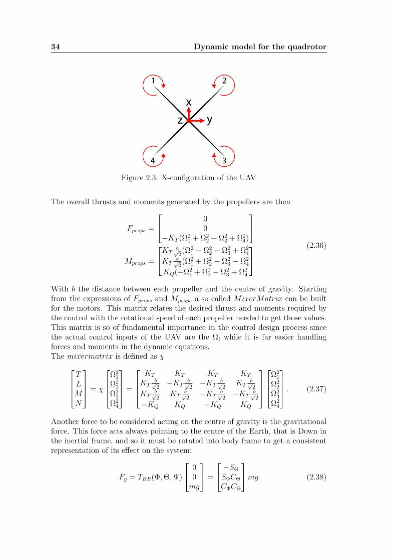
In the study of the UAV dynamics it is necessary to analyse the external forces andmoments introduced in the previous sections in order to get a correct modellingof the system. The quadrotor studied is set in X-configuration (see Figure 2.3).Each propeller produces a torque and a thrust proportional to the square of itsrotational speed:

Ti = KTΩ2i , KT = CTρAR

2,

Qi = KQΩ2i , KQ = CQρAR

3,(2.35)

Where CT and CQ are the thrust and torque coefficients, ρ the air density, A andR the propeller disk and its radius and Ωi is the i-th propeller rotational speed.


Figure 2.3: X-configuration of the UAV

The overall thrusts and moments generated by the propellers are then

Fprops =

00

−KT (Ω21 + Ω2

2 + Ω23 + Ω2

4)

Mprops =

KTb√2(Ω2

1 − Ω22 − Ω2

3 + Ω24

KTb√2(Ω2

1 + Ω22 − Ω2

3 − Ω24

KQ(−Ω21 + Ω2

2 − Ω23 + Ω2

4

(2.36)

With b the distance between each propeller and the centre of gravity. Startingfrom the expressions of Fprops and Mprops a so called MixerMatrix can be builtfor the motors. This matrix relates the desired thrust and moments required bythe control with the rotational speed of each propeller needed to get those values.This matrix is so of fundamental importance in the control design process sincethe actual control inputs of the UAV are the Ωi while it is far easier handlingforces and moments in the dynamic equations.The mixermatrix is defined as χ

TLMN

= χ

Ω2

1

Ω22

Ω23

Ω24

=

KT KT KT KT

KTb√2−KT

b√2−KT

b√2

KTb√2

KTb√2

KTb√2−KT

b√2−KT

b√2

−KQ KQ −KQ KQ

Ω21

Ω22

Ω23

Ω24

. (2.37)

Another force to be considered acting on the centre of gravity is the gravitationalforce. This force acts always pointing to the centre of the Earth, that is Down inthe inertial frame, and so it must be rotated into body frame to get a consistentrepresentation of its effect on the system:

Fg = TBE(Φ,Θ,Ψ)

00mg

=

−SΘ

SΦCΘ

CΦCΘ

mg (2.38)

2.4 Conclusions 35

The last effect to consider is the aerodynamic damp caused by the rotating pro-pellers moving through air. Assuming in first approximation the drag caused bylinear translations to be negligible since the structure of the quadrotor is thin, themoments around each axis are only proportional to the rotational speed aroundthat axis (decoupled moments). Moreover, if one considers only the aerodynamicdamp proportional to ωb it takes the form

Mdamp =

∂L∂p 0 0

0 ∂M∂q

0

0 0 ∂N∂r

pqr

. (2.39)

The terms ∂L∂p

, ∂M∂q

, ∂N∂r

are called stability derivatives. Because of the symmetry

of the UAV ∂L∂p

= ∂M∂q

, while ∂N∂r

= 0 since the angular rate about the Z axis isfar lower than the others. The stability derivatives are defined from helicopterstheory as

∂L

∂p= −4ρAR2Ω2∂CT

∂p

b√2

(2.40)

∂CT∂p

=CLα

8

σ

RΩ

b√2

(2.41)

σ =AbA

(2.42)

with σ called solidity ratio obtained dividing the blade area Ab over the disk areaA. CLα is defined as the slope of the thrust coefficient curve CL, this parameteris assumed to be 2π since the actual air-foil is not known and the propeller bladeis thin.All the values of the aerodynamic and structural parameters of the drone havebeen inherited from [4] and [3] where all the unknown values have been identifiedusing grey-box estimation.In the end the total forces and moments applied to the centre of mass of the UAVare described by:

Fext = Fg + Fprops

Mext = Mdamp +Mprops.(2.43)

2.4 Conclusions

The conventions and the UAV model as been presented in detail in this chapter,highlighting all the modelling assumptions and the implication they have in thefinal result.The final model to be controlled is then

mVb + ωb × (mVb) = Fg + Fprops

Inωb + ωb × (Inωb) = Mdamp +Mprops.(2.44)


Starting from this model a Simulink simulator for the system has been developedin [4] and it has been used extensively in the process of control synthesis andvalidation. During the development of this thesis some adjustments have beenadded improving the coherence with the real behaviour of a quadrotor helicopter.

Chapter 3

Control design and tuning

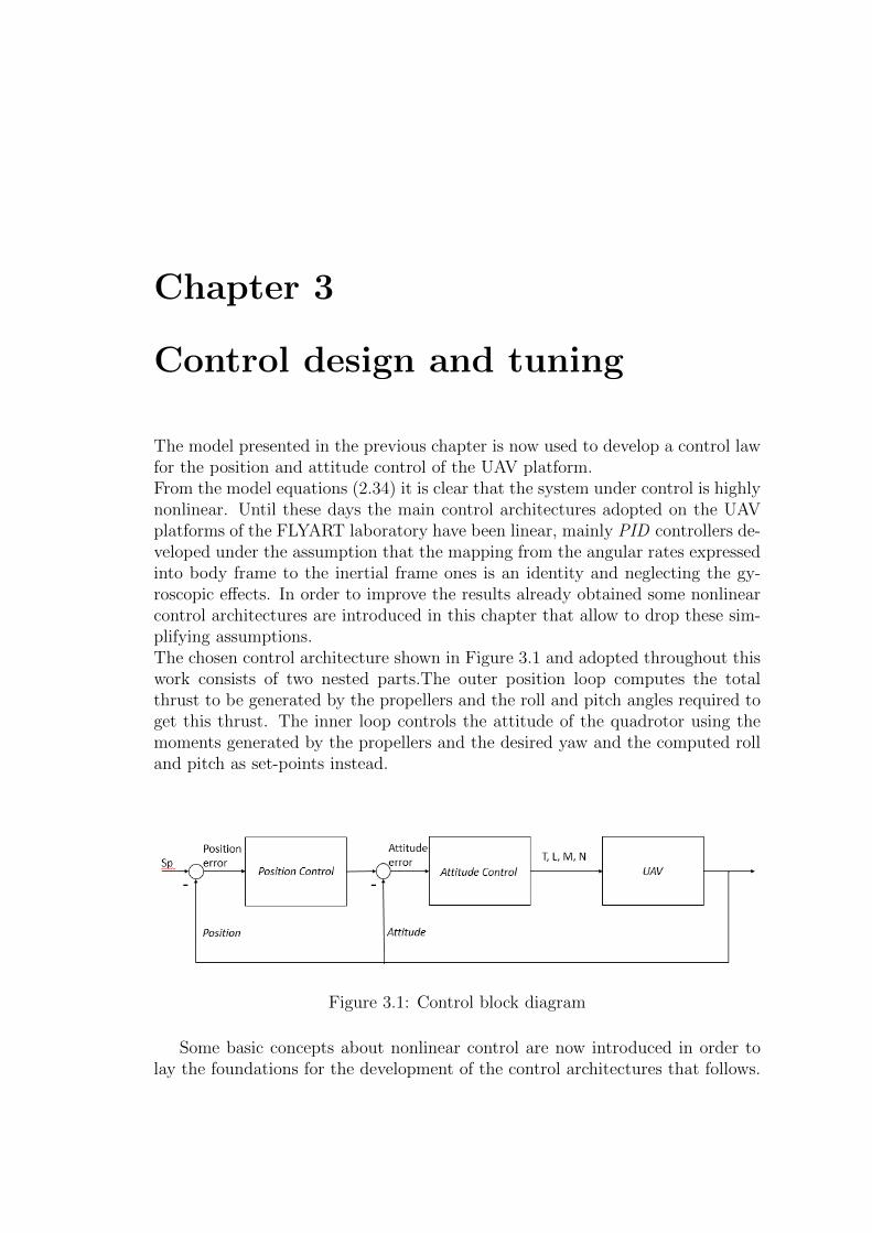
The model presented in the previous chapter is now used to develop a control lawfor the position and attitude control of the UAV platform.From the model equations (2.34) it is clear that the system under control is highlynonlinear. Until these days the main control architectures adopted on the UAVplatforms of the FLYART laboratory have been linear, mainly PID controllers de-veloped under the assumption that the mapping from the angular rates expressedinto body frame to the inertial frame ones is an identity and neglecting the gy-roscopic effects. In order to improve the results already obtained some nonlinearcontrol architectures are introduced in this chapter that allow to drop these sim-plifying assumptions.The chosen control architecture shown in Figure 3.1 and adopted throughout thiswork consists of two nested parts.The outer position loop computes the totalthrust to be generated by the propellers and the roll and pitch angles required toget this thrust. The inner loop controls the attitude of the quadrotor using themoments generated by the propellers and the desired yaw and the computed rolland pitch as set-points instead.

Figure 3.1: Control block diagram

Some basic concepts about nonlinear control are now introduced in order tolay the foundations for the development of the control architectures that follows.

38 Control design and tuning

3.1 Lyapunov stability theory

In the case a nonlinear system cannot be linearised around an equilibrium or ifthis approximation is too strong, one of the most used control methods is the socalled Lyapunov method, from the name of Aleksandr Michajlovic Lyapunov whotheorized it first.The main idea underlying this approach is that if the total energy of the systemunder control is continuously dissipated, at least in the neighbourhood D of anequilibrium x0, the system tends to move to the equilibrium itself.In the first place an energy function must be defined. This function V has to be

• positive definite for all x 6= 0 with x ∈ D

• V (x) = 0 if and only if x = 0

If the derivative of V (x) along the trajectories of the system is negative definite, orat least negative semi-definite and null only in x = 0, the energy is continuouslydissipated by the system or it does not increase and can only be conserved ordissipated. This fact leads to the Lyapunov theorem for nonlinear systems: givena system x(t) = φ(x(t)) with φ continuous with its derivative and locally Lipschitzin a neighbourhood D of a considered equilibrium x0, if there exists a functionV (x), continuous with its derivative, positive definite in x0 and such that V (x) issemi-definite negative around x0, that is

V (x) =dV

dx

dx

dt=dV

dxφ(x) ≤ 0 x ∈ D (3.1)

then x0 is a stable equilibrium, see [8] for the complete proof.Moreover if V (x) < 0 strictly, that is V (x) negative definite, x0 is an asymptoti-cally stable equilibrium.Another theorem, the Krasowsky - La Salle Lemma, proves that in addition tothe previous cases if V (x) ≤ 0 but V (x) = 0 only in x = x0 then the equilibriumis asymptotically stable also in this case.Based on the results of these theorems, many control strategies for nonlinear sys-tems have been built.Once a suitable energy function V (x) has been found, with x the states of thesystem to be controlled, a stabilizing control input that forces its derivative to benegative definite is computed.

3.1.1 The backstepping method

One possible way to compute the control variable is the so called backsteppingmethod.

3.1 Lyapunov stability theory 39

The general idea behind this technique can be easily explained by means of anexample. Given a system with two states x1, x2 in the form:

x1 = f(x1) + gx2 x1 ∈ Rn x2 ∈ Rx2 = u

(3.2)

Where f is continuous and differentiable in a set D ⊂ Rn and f(0) = 0 whileg ∈ Rn×1 constant, and u is the control variable of our system. The objective isto stabilize the system around its equilibrium x1 = 0, x2 = 0.To do so temporarily assume that x2 is a free design variable and to be able tostabilize the first equation of the system with the control law:

x2 = Φ(x1), Φ(0) = 0. (3.3)

Adopting this control law the closed loop system is

x1 = f(x1) + gΦ(x1). (3.4)

Assume to know a Lyapunov function V1(x1) such that:

V1(x1) =dV1

dx1

(f(x1) + gΦ(x1)) = −W (x1) (3.5)

where W (x1) > 0 for any x1 ∈ D.At this point it has to be considered that the state x2 has its own dynamic andcannot be freely chosen, so it is possible to define the error between the actualand the desired behaviour of x2, as follows

η = x2 − Φ(x1), Φ(0) = 0. (3.6)

The derivative of η is then

η = x2 − Φ(x1)

= u− dΦ(x1)

dx1

x1

= u− dΦ(x1)

dx1

[f(x1) + g

(η + Φ(x1)

)].

(3.7)

Therefore the initial system can be reformulated asx1 = f(x1) + g

[η + Φ(x1)

]η = u− dΦ(x1)

dx1

[f(x1) + g

(η + Φ(x1)

)].

(3.8)

It is now possible to define a new input

v = u− Φ(x1). (3.9)


It is quite evident that η = v, and the system can be given the formx1 = f(x1) + gΦ(x1) + gη

η = v(3.10)

where the origin is an asymptotically stable equilibrium for the first subsystem.Consider the following Lyapunov function for the overall system

V2(x1, η) = V1(x1) +1

2η2 (3.11)

and its derivative

V2(x1, η) =dV1

dx1

x1 + ηη

=dV1

dx1

(f(x1) + gΦ(x1) + gη

)+ ηv

≤ −W (x1) +dV1

dx1

gη + ηv

(3.12)

Therefore, by imposing

v = −dV1

dx1

g − kη k > 0 (3.13)

it follows thatV2(x1, η) = −W (x1)− kη2 < 0, (3.14)

thus the equilibrium (x1 = 0, η = 0) is an asymptotically stable equilibrium of thesystem. Recalling that η = x2−Φ(x1) and Φ(0) = 0 it follows that (x1 = 0, x2 = 0)is an asymptotically stable equilibrium.One can compute the expression of the control law for u that stabilizes the originas function of the original coordinates as

u = v + Φ(x1)

= −dV1

dx1

g − k(x2 − Φ(x1)

)+ Φ(x1) +

dΦ(x1)

dx1

(f(x1) + gx2

) (3.15)

This control law guarantees the asymptotic stability of the origin, with the asso-ciated Lyapunov function

V2(x1, x2) = V1(x1) +1

2

(x2 − Φ(x1)

)2. (3.16)

Thus it is possible to consider a state as a virtual control variable that stabilizesthe other states, then back-compute the required control law in order to force thatstate to stabilize the others.For the general formulation and a deeper insight on this technique see [8] .

3.2 Backstepping control of a UAV quadrotor 41

3.2 Backstepping control of a UAV quadrotor

In this section the derivation of the backstepping control algorithm for the UAVplatform is carried out.In first instance the derivation of the attitude control law is explained, all thecomputations are carried out considering only one degree of freedom of the sys-tem and then the final results are extended to the others. Then the derivation ofthe position control algorithm is introduced. All the procedure has been faced in[1].

3.2.1 Derivation of the attitude control law

Starting from (2.44) and (2.34) , one can extract the equations of the attitudedynamics:

pqr

Φ

Θ

Ψ

=

(I−1n (−ωb × Inωb +Mext)

E−1ωb

). (3.17)

The resulting equations of the attitude dynamics turn out to be:

p = I−1xx

[(Iyy − Izz)qr +

∂L

∂pp+ L

]q = I−1

yy

[(Izz − Ixx)pr +

∂M

∂qq +M

]r = I−1

zz

[(Ixx − Iyy)pq +

∂N

∂rr +N

].

(3.18)

Assuming that the rotation axes are decoupled (E−1 = I ) one has that

Φ

Θ

Ψ

=

pqr

(3.19)

and applying to the dynamics of each Euler angle the 1-degree of freedomapproximation we can directly access the roll, pitch and yaw dynamics startingfrom the angular rates dynamics expressed in body reference frame. All these


assumptions are widely used in the literature and lead to the model

Φ = I−1xx

[(Iyy − Izz)ΘΨ +

∂L

∂pΦ + L

]Θ = I−1

yy

[(Izz − Ixx)ΦΨ +

∂M

∂qΘ +M

]Ψ = I−1

zz

[(Ixx − Iyy)ΦΘ +

∂N

∂rΨ +N

].

(3.20)

From equation (3.20) the objective is now to find a way to control the attitudeof the UAV so that it can reach any desired attitude (excluding the singularitiesof the representation) in a fast and stable manner.In order to do so a new system can be built that considers the dynamics of theattitude errors. If a stabilizing control law for the origin of the states of thissystem is achieved, it is possible to set the quadrotor at any desired attitude.From now on all the computations are developed for one of the three coordinatesand the final results for all coordinates are shown at the end of the section.The first step is to define the attitude error

eΦ = Φdes − Φ (3.21)

and then compute the dynamics of the chosen Lyapunov function and find anequation for the control variable that stabilizes the function dynamics.

VΦ =1

2e2

Φ

VΦ(eΦ) = eΦ(Φdes − Φ)(3.22)

In order to get Lyapunov stability for the origin, the derivative along thetrajectories of the Lyapunov function has to be negative definite (or at leastnegative semi-definite with the only acceptable root of the function in the origin).This can be achieved setting

Φ = Φdes + α1eΦ

VΦ(eΦ) = −α1e2Φ

(3.23)

with α1 > 0 free control parameter to be tuned that affects the convergence tozero of the error dynamics. The convergence of Φ to the desired value that ensuresthe control of the roll angle dynamics must now be studied. To do so we extendthe previous Lyapunov function including also the dynamics of the roll rate erroreΦ defined as

eΦ = Φ− Φdes − α1eΦ (3.24)

The extended Lyapunov function takes the form

VΦ(eΦ, eΦ) =1

2(e2

Φ + e2Φ

) (3.25)

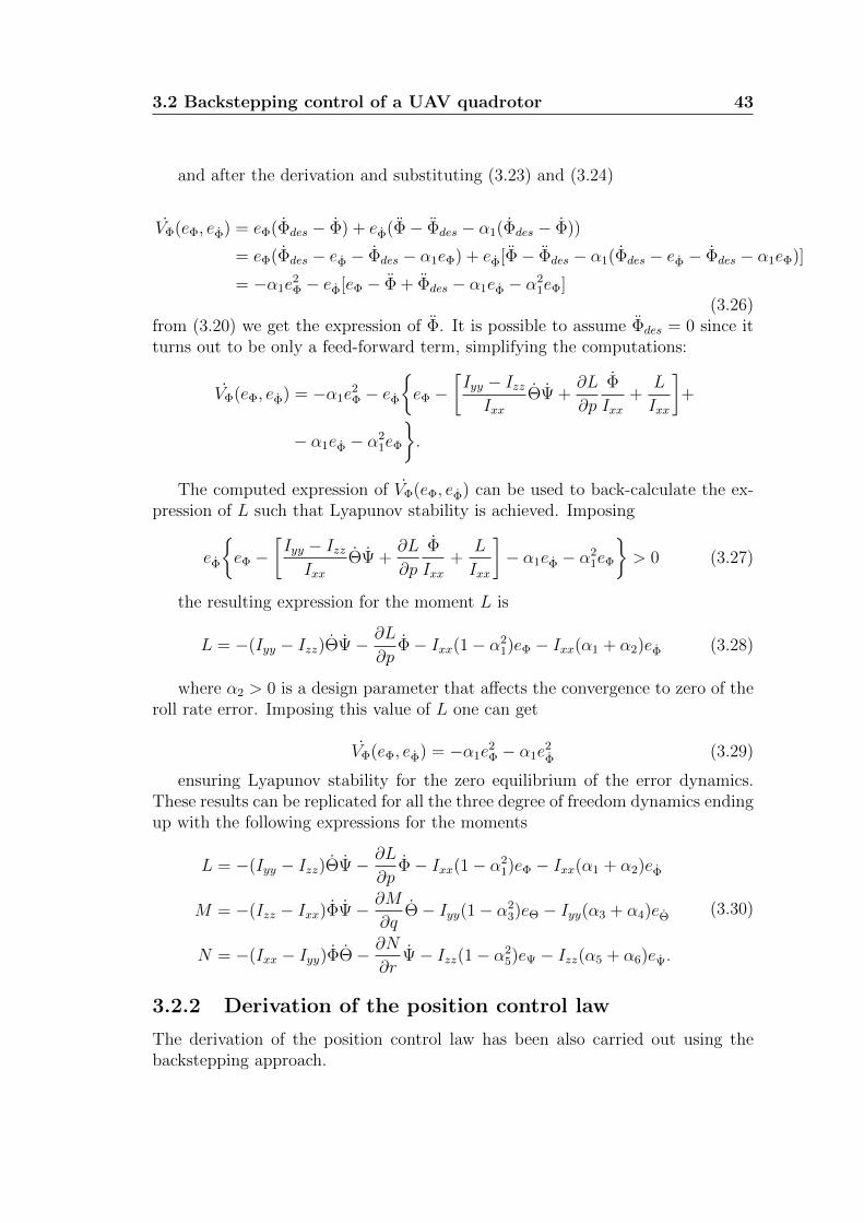
3.2 Backstepping control of a UAV quadrotor 43

and after the derivation and substituting (3.23) and (3.24)

VΦ(eΦ, eΦ) = eΦ(Φdes − Φ) + eΦ(Φ− Φdes − α1(Φdes − Φ))

= eΦ(Φdes − eΦ − Φdes − α1eΦ) + eΦ[Φ− Φdes − α1(Φdes − eΦ − Φdes − α1eΦ)]

= −α1e2Φ − eΦ[eΦ − Φ + Φdes − α1eΦ − α

21eΦ]

(3.26)from (3.20) we get the expression of Φ. It is possible to assume Φdes = 0 since itturns out to be only a feed-forward term, simplifying the computations:

VΦ(eΦ, eΦ) = −α1e2Φ − eΦ

eΦ −

[Iyy − IzzIxx

ΘΨ +∂L

∂p

Φ

Ixx+

L

Ixx

]+

− α1eΦ − α21eΦ

.

The computed expression of VΦ(eΦ, eΦ) can be used to back-calculate the ex-pression of L such that Lyapunov stability is achieved. Imposing

eΦ

eΦ −

[Iyy − IzzIxx

ΘΨ +∂L

∂p

Φ

Ixx+

L

Ixx

]− α1eΦ − α

21eΦ

> 0 (3.27)

the resulting expression for the moment L is

L = −(Iyy − Izz)ΘΨ− ∂L

∂pΦ− Ixx(1− α2

1)eΦ − Ixx(α1 + α2)eΦ (3.28)

where α2 > 0 is a design parameter that affects the convergence to zero of theroll rate error. Imposing this value of L one can get

VΦ(eΦ, eΦ) = −α1e2Φ − α1e

2Φ

(3.29)

ensuring Lyapunov stability for the zero equilibrium of the error dynamics.These results can be replicated for all the three degree of freedom dynamics endingup with the following expressions for the moments


∂pΦ− Ixx(1− α2

1)eΦ − Ixx(α1 + α2)eΦ

M = −(Izz − Ixx)ΦΨ− ∂M

∂qΘ− Iyy(1− α2

3)eΘ − Iyy(α3 + α4)eΘ

N = −(Ixx − Iyy)ΦΘ− ∂N

∂rΨ− Izz(1− α2

5)eΨ − Izz(α5 + α6)eΨ.

(3.30)

3.2.2 Derivation of the position control law

The derivation of the position control law has been also carried out using thebackstepping approach.


While the altitude control law derivation follows exactly the same path of theattitude one, the x, y axes controls are used to compute the desired roll and pitchangles and thus the derivation is slightly different.The considered dynamic model can be extracted from (2.44) and (2.34) and takesthe form:

x =(cΦsΘcΨ + sΦsΨ

)(−Tm

)y =

(cΦsΘsΨ − sΦcΨ

)(−Tm

)z = cΦcΘ

(−Tm

)+ g.

(3.31)

The first step is to compute the total thrust T required to get the desired altitude.Defining the altitude error ez and the candidate Lyapunov function Vz as

ez = zdes − z

Vz =1

2e2z

(3.32)

the derivative of Vz can be easily computed as

Vz(ez) = ez(zdes − z). (3.33)

Following the backstepping logic the state z can be chosen as virtual controlvariable and then its value should be

zv = zdes + α7ez (3.34)

Then the extended Lyapunov function V (ez, ez) is defined as

ez = z − zdes − α7ez

Vz(ez, ez) =1

2(e2z + e2

z).(3.35)

It is now possible to find the total thrust to be applied in order to get the desiredequation following the same procedure used in (3.26) and imposing Vz ≤ 0.The resulting total thrust is then:

T =m

CΦCΘ

[g + (α7 + α8)ez + (α2

7 − 1)ez

]. (3.36)

Where α7,8 > 0 are control parameters to be tuned.Once the expression of T for the altitude control is fixed, the x, y controls aim atcomputing the desired values of roll and pitch in order to direct the thrust correctlyconsidering that the desired yaw is set by the user. The model as presented in(3.31) is in the form

x =(cΦsΘcΨ + sΦsΨ

)(−Tm

)y =


)(−Tm

) (3.37)

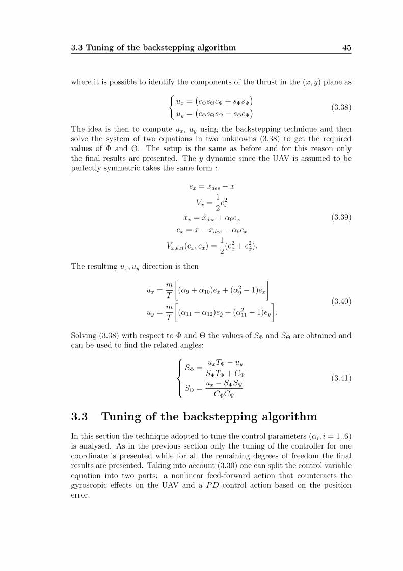
3.3 Tuning of the backstepping algorithm 45

where it is possible to identify the components of the thrust in the (x, y) plane asux =

(cΦsΘcΨ + sΦsΨ

)uy =


) (3.38)

The idea is then to compute ux, uy using the backstepping technique and thensolve the system of two equations in two unknowns (3.38) to get the requiredvalues of Φ and Θ. The setup is the same as before and for this reason onlythe final results are presented. The y dynamic since the UAV is assumed to beperfectly symmetric takes the same form :

ex = xdes − x

Vx =1

2e2x

xv = xdes + α9ex

ex = x− xdes − α9ex

Vx,ext(ex, ex) =1

2(e2x + e2

x).

(3.39)

The resulting ux, uy direction is then

ux =m

T

[(α9 + α10)ex + (α2

9 − 1)ex

]uy =

m

T

[(α11 + α12)ey + (α2

11 − 1)ey

].

(3.40)

Solving (3.38) with respect to Φ and Θ the values of SΦ and SΘ are obtained andcan be used to find the related angles:

SΦ =uxTΨ − uySΨTΨ + CΨ

SΘ =ux − SΦSΨ

CΦCΨ

(3.41)

3.3 Tuning of the backstepping algorithm

In this section the technique adopted to tune the control parameters (αi, i = 1..6)is analysed. As in the previous section only the tuning of the controller for onecoordinate is presented while for all the remaining degrees of freedom the finalresults are presented. Taking into account (3.30) one can split the control variableequation into two parts: a nonlinear feed-forward action that counteracts thegyroscopic effects on the UAV and a PD control action based on the positionerror.


In fact we can rearrange the expression of L as


∂pΦ︸︷︷︸

Nonlinear FF

+ L′︸︷︷︸PD action

(3.42)

With L′ in the form

L′ = −Ixx(1− α21)eΦ︸︷︷︸

Proportional action

−Ixx(α1 + α2)eΦ︸︷︷︸Derivative action

(3.43)

Substituting in (3.43) the expressions of eΦ, eΦ in (3.23) and (3.24) we can rear-range its expression as

L′ = −Ixx[(α21 − 1− α1α2 − α2

1)(Φdes − Φ)− (α1 + α2)(Φdes − Φ)]

= Ixx[(1 + α1α2)eΦ + (α1 + α2)eΦ]

= KPΦeΦ +KDΦeΦ

KPΦ = Ixx(1 + α1α2)

KDΦ = Ixx(α1 + α2)

(3.44)

From this results it is clear that one can deal with the control tuning problem asa PD control tuning task assuming the perfect compensation of the feed-forwardterms. The aim of the procedure outlined in the following is to find optimal valuesfor α1, α2 exploiting the fact that the analytical relation between them and theirequivalent effect in a linear controller is available.To do so the structured mixed sensitivity H∞ technique has been adopted ap-plying it to the system linearised around each rotation axes. The controller isthus parametrised as function of α1, α2 leaving the solution of the nonlinear rela-tion between α1, α2 and KPΦ, KDΦ to the optimization algorithm. The linearisedsystem takes the form

Φ = I−1xx L

Θ = I−1yy M

Ψ = I−1zz N

(3.45)

which can be rewritten as

φ = I−1xx

[1

s2

]L

θ = I−1yy

[1

s2

]M

ψ = I−1zz

[1

s2

]N .

(3.46)


The starting point is then a double integrator since the stability derivativesare assumed to be perfectly compensated by the feedforward. In order to get amore consistent model and a more robust tuning (3.46) has been cascaded withthe model of the actuators identified in [4] and analysed in 4.1.2 and a delayof 0.02[s] representing the sensors and the attitude determination system. Theresulting closed-loop system, the control law, the sensors and actuators, the lin-earised quadrotor has been fed to the Systune function provided by the Matlabenvironment.

3.3.1 Shaping functions

One of the key aspects of the structured H∞ tuning technique is the choice of theshaping functions to be fed to the optimization algorithm in order to achieve thetuning of the control parameters.The objective of mixed-sensitivity synthesis is to keep the the H∞-norm of theproduct between the sensitivity, complementary sensitivity and control sensitivityfunctions of the system with the shaping functions as close as possible to 1, thatis

||WS(s)S(s)||∞ ≤ 1

||WT (s)T (s)||∞ ≤ 1

||WK(s)K(s)||∞ ≤ 1.

(3.47)

Thus each weight has a specific meaning and has to be chosen following someguidelines that have been derived from [10] .

• WS(s) weights the sensitivity of the system to external disturbances on theoutput. Namely it is the transfer function from disturbance on the outputto the output itself. It has to be chosen high at low frequency in order toget a strong attenuation of the disturbances in the bandwidth of interest(below the frequency ωB) and around 0dB at high frequency. The optimalvalue of 0dB at high frequency usually is not a good choice since there isquite often a resonance peak around ωB, thus choosing WS(ωB) = 0 makesthe algorithm try to push the resonance down and so it strongly limits theoverall performances of the resulting control, however the high frequencyvalue must be kept low in order to damp the dominant pole of the system.The theory, see [8], suggests that the overall crossover frequency ωc of thecontrolled system is higher that ωB. The inverse of the chosen function isshown in Figure 3.2 and guarantees ωc ≥ 3 [rad/s].

• WT (s) weights the complementary sensitivity function, that affects the ro-bustness properties of the system. Since the uncertainties on the modelparameters are low due to various identification campaigns (see [4] and [3])this function has been used in order to enforce a consistent upper bound to


Figure 3.2: Magnitude of the frequency response of inverse of the chosen WS(s)function

the ωc since ωB ≤ ωc ≤ ωBT with ωBT the crossover frequency of WT (s) .Since the complementary sensitivity function is 1 − S(s) the magnitude ofWT (jω) will be around 0dB at low frequency, decreases for higher frequen-cies and has a cutting frequency ωBT = 7 [rad/s]as one can deduce fromFigure 3.3 in which the magnitude of the frequency response of the inverseof WT (s) is shown.

• WK(s) weights the control sensitivity function K(s). The K(s) function canbe seen as the transfer function

– from reference signal to control action;

– from disturbance on the output to control action;

– from measurement noise to control action.

In all these cases, it is desirable to keep the magnitude of the control sensi-tivity frequency response as small as possible outside the bandwidth of thesystem.WK(s) have also to keep into account physical restrictions of the system,that is the bandwidth of the actuators and the maximum deliverable mo-ments. For all these reasons the selected weighting function has a cuttingfrequency of ωBK = 18.09[rad/s] and a shape that can be deduced from themagnitude of the frequency response of its inverse shown in Figure 3.4 .


Figure 3.3: Magnitude of the frequency response of inverse of the chosen WT (s)function

Figure 3.4: Magnitude of the frequency response of inverse of the chosen WK(s)function


Table 3.1: Outer loop shaping functions parameters, backstepping

ωB[rad/s] ωBT [rad/s] ωBK [rad/s]

0.1 0.2 18.09

Once established all these requirements, the shaping functions have been builtup using first order functions and have been used for the tuning of each of theattitude controllers.The same approach has been adopted for the tuning of the position control loop,following exactly the same steps and considering the inner loop to be a unitarygain since quite faster then the outer one. The inverses of the chosen weightingfunctions are shown in Figure 3.5 with the characteristics in Table 3.1

Figure 3.5: Magnitude of the frequency response of the inverse outer loop weight-ing functions, backstepping

3.3.2 Tuning results

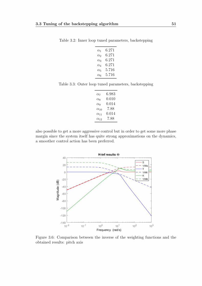
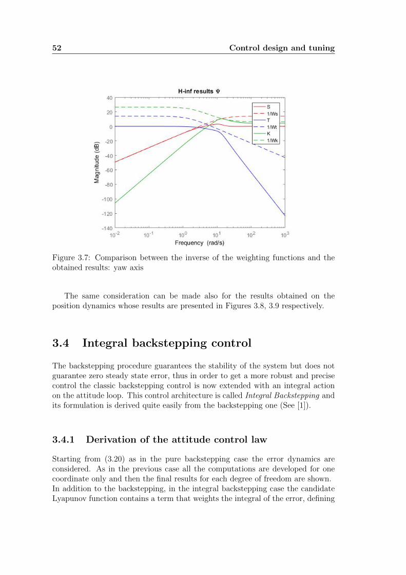
The resulting tuning of the parameters for the inner and outer loops is shown inTables 3.2, 3.3 respectively.Figures 3.6, 3.7 show the results of the H∞ tuning procedure for the pitch andyaw dynamics comparing the shaping functions presented before with the obtainedS(s), T (s), K(s) of the tuned systems. It is easy to see that the tuning procedurehas led to good tuning results, at least with the linearised system. In principle it is


Table 3.2: Inner loop tuned parameters, backstepping

α1 6.271α2 6.271α3 6.271α4 6.271α5 5.716α6 5.716

Table 3.3: Outer loop tuned parameters, backstepping

α7 6.983α8 0.010α9 0.014α10 7.88α11 0.014α12 7.88

also possible to get a more aggressive control but in order to get some more phasemargin since the system itself has quite strong approximations on the dynamics,a smoother control action has been preferred.

Figure 3.6: Comparison between the inverse of the weighting functions and theobtained results: pitch axis


Figure 3.7: Comparison between the inverse of the weighting functions and theobtained results: yaw axis

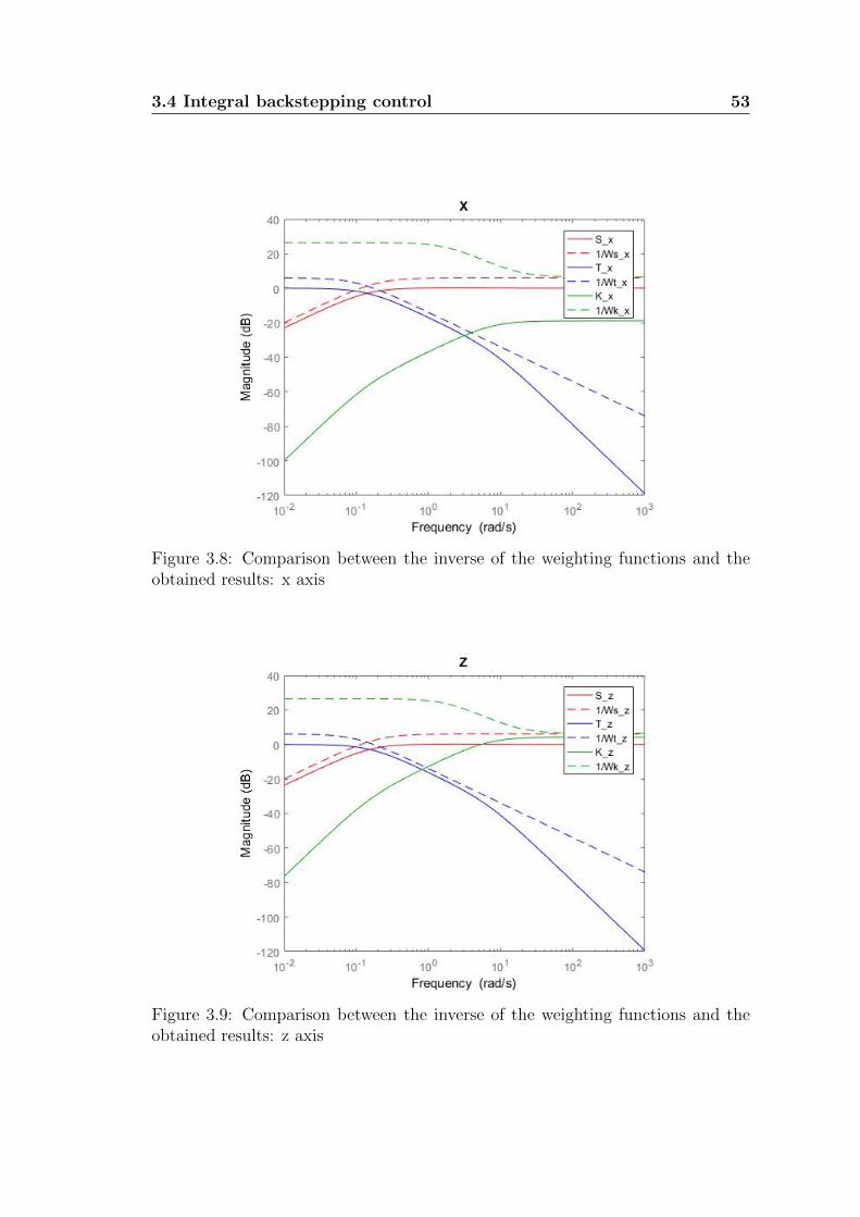
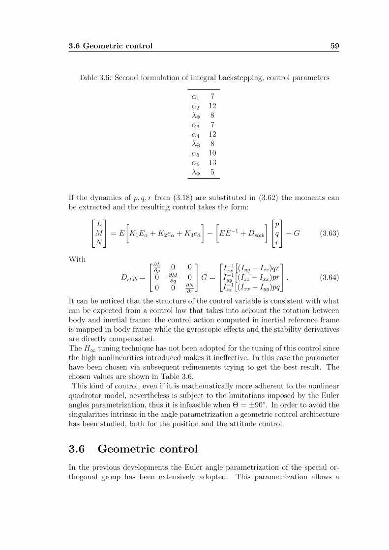
The same consideration can be made also for the results obtained on theposition dynamics whose results are presented in Figures 3.8, 3.9 respectively.

3.4 Integral backstepping control

The backstepping procedure guarantees the stability of the system but does notguarantee zero steady state error, thus in order to get a more robust and precisecontrol the classic backstepping control is now extended with an integral actionon the attitude loop. This control architecture is called Integral Backstepping andits formulation is derived quite easily from the backstepping one (See [1]).


Starting from (3.20) as in the pure backstepping case the error dynamics areconsidered. As in the previous case all the computations are developed for onecoordinate only and then the final results for each degree of freedom are shown.In addition to the backstepping, in the integral backstepping case the candidateLyapunov function contains a term that weights the integral of the error, defining

3.4 Integral backstepping control 53

Figure 3.8: Comparison between the inverse of the weighting functions and theobtained results: x axis

Figure 3.9: Comparison between the inverse of the weighting functions and theobtained results: z axis


the attitude error eΦ and its integral EΦ it takes the form

eΦ = Φdes − Φ

EΦ =

∫eΦ

VΦ =1

2(e2

Φ + λΦE2Φ)

(3.48)

with λΦ parameter to be tuned.The virtual control ΦV is then computed in order to keep the derivative of VΦ < 0

VΦ(eΦ, EΦ) = eΦ(Φdes − Φ + λΦEΦ)

ΦV = Φdes + λΦEΦ + α1eΦ.(3.49)

The next step is to extend the Lyapunov function in order to consider that ourcontrol variable is not the virtual control one, leading to an error that mustconverge to zero:

VΦ(eΦ, eΦ, EΦ) =1

2(e2

Φ + e2Φ

+ λΦE2Φ)

eΦ = ΦV − Φ = Φdes + λΦEΦ + α1eΦ − Φ

Φ = Φdes + λΦEΦ + α1eΦ − eΦ.

(3.50)

The derivative of this extended Lyapunov function is then

VΦ(eΦ, eΦ, EΦ) = eΦeΦ + λΦEΦeΦ + eΦeΦ

eΦ = Φdes − Φ = eΦ − λΦEΦ − α1eΦ

eΦ = α1(eΦ − λΦEΦ − α1eΦ) + λΦeΦ + Φdes − Φ.

(3.51)

Substituting all the terms it is possible to get:

VΦ(eΦ, eΦ, EΦ) = eΦ(eΦ − λΦEΦ − α1eΦ) + λΦEΦeΦ

+ eΦ[α1(eΦ − λΦEΦ − α1eΦ) + λΦeΦ + Φdes − Φ].(3.52)

Imposing VΦ = −α1e2Φ−α2e

2Φ

one can extract the required value of the accelerationthat is:

Φ = (1 + λΦ − α21)eΦ + (α1 + α2)eΦ − λΦα1EΦ + Φdes. (3.53)

Then substituting the expression of the angular acceleration from (3.20) and as-suming Φdes = Θdes = Ψdes = 0 the control moments are obtained:


∂pΦ + Ixx[(1 + λΦ − α2

1)eΦ + (α1 + α2)eΦ − λΦα1EΦ]

M = −(Izz − Ixx)ΦΨ− ∂M

∂qΘ + Iyy[(1 + λΘ − α2

3)eΘ + (α3 + α4)eΘ − λΘα3EΘ]

N = −(Ixx − Iyy)ΦΘ− ∂N

∂rΨ + Izz[(1 + λΨ − α2

5)eΨ + (α5 + α6)eΨ − λΨα5EΨ].

(3.54)

3.4 Integral backstepping control 55

Table 3.4: Outer loop shaping functions parameters, integral backstepping

ωB[rad/s] ωBT [rad/s] ωBK [rad/s]

4.5 6.5 18.09

Table 3.5: Outer loop tuned parameters, integral backstepping

α1 7.3033α2 7.3007λΦ 0.010α3 7.3033α4 7.3007λΘ 0.010α5 2.0960α6 6.3184λΦ 20.613

3.4.2 Tuning of the integral backstepping control law

Like the previous case the control expression can be divided into two parts: anonlinear feedforward that compensates the gyroscopic effects and the stabilityderivatives, and a control action that depends on the errors and the control pa-rameters to be tuned.Expanding eΦ as in the previous case the expression turns out to be a PID con-troller:

L = −(Iyy−Izz)ΘΨ− ∂L∂p

Φ+Ixx[λΦα2EΦ+(1+λΦ−α1α2)eΦ+(α1+α2)eΦ] (3.55)

So, as in the classical backstepping architecture we can consider the control actionas a PID with gains that depend on the Lyapunov parameters:

KI = IxxλΦα2

KP = Ixx(1 + λΦ − α1α2)

KD = Ixx(α1 + α2)

(3.56)

The so obtained control law has been tuned using the H∞ technique described insection 3.3 using the shaping functions whose parameters are described in Table3.4 and depicted in Figure 3.10. Also in this case the Systune routine has beenadopted and leads to a satisfactory tuning as can be seen in Figure 3.11 regardingthe pitch dynamics and in Figure 3.12 for the yaw one.

The resulting Lyapunov parameters that have been found in this way aresummarized in Table 3.5. It is quite evident that with respect to the pure back-stepping, in this case ωB has been set to 4.5 [rad/s], that is quite faster, and as a


Figure 3.10: Magnitude of the frequency response of the inverse shaping functionsfor integral backstepping control tuning

Figure 3.11: Results of the H∞ tuning for the integral backstepping controller:pitch axis

3.5 Second formulation of integral backstepping 57

Figure 3.12: Results of the H∞ tuning for the integral backstepping controller:yaw axis

result the value of the gains increases.

3.5 Second formulation of integral backstepping

At the beginning of the chapter the assumption E ≈ I has been introduced, thatallows to consider the effect of the body angular rate affecting only one coordinatein NED reference frame.This strong assumption limits the effectiveness of the control to certain range ofangles and can lead to unstable behaviours of linear controllers in the case of veryaggressive manoeuvres. In order to get a better control action, the previous as-sumption has been dropped and a new controller based the integral backsteppingtechnique has been developed.


The idea behind this modification of the integral backstepping is quite simple, thesmall angle approximation that lead to E ≈ I is dropped, and so while controllingthe attitude error dynamics the control action is considered on the body angularrate ωb and not directly on the attitude angles rates.


The first steps and the derivation is analogous to the integral backstepping oneshown in equations (3.48) and (3.49), from those expressions the virtual controlΦV is computed

ΦV = Φdes + λΦEΦ + α1eΦ. (3.57)

Now the convergence of the extended Lyapunov function has to be studied. As inequation (3.50) the error on the angular rate has to be defined:

eΦ = ΦV − Φ = Φdes + λΦEΦ + α1eΦ − Φ

VΦ(eΦ, eΦ, EΦ) =1

2(e2

Φ + e2Φ

+ λΦE2Φ)

VΦ(eΦ, eΦ, EΦ) = eΦeΦ + λΦEΦeΦ + eΦeΦ

(3.58)

and after some computation the expression of VΦ can be obtained in the form

VΦ = −α1e2Φ + eΦ

(eΦ + λΦeΦ − λΦα1EΦ − α2

1eΦ + α1eΦ − Φ

). (3.59)

The expression of Φ can be substituted taking into account thatΦ

Θ

Ψ

= E−1

pqr

Φ

Θ

Ψ

= E−1

pqr

+ E−1

pqr

(3.60)

and imposing VΦ = −α1e2Φ−α2e

2Φ

it is possible to work out the following equationin three unknowns

eΦ + λΦeΦ − λΦα1EΦ − α21eΦ + α1eΦ + α2eΦ = E−1

(1,:)

pqr

+ E−1(1,:)

pqr

, (3.61)

where E−1(1,:), E

−1(1,:) are the first rows of the two matrices. It is quite clear that

in this case the control action can be computed only taking into account all thethree coordinates, intuitively because this algorithm takes into account also thecoupling between the axes. For all the other coordinates the computation untilthis point are the same and the resulting system can take the form

E−1

pqr

= K1

EΦ

EΘ

EΨ

+K2

eΦ

eΘ

eΨ

+K3

eΦ

eΘ

eΨ

− E−1

pqr

K1 = diag(λΦα1, λΘα3, λΨα5);

K2 = diag((1 + λΦ − α21), (1 + λΘ − α2

3), (1 + λΨ − α25));

K1 = diag((α1 + α2), (α3 + α4), (α5 + α6));

(3.62)

3.6 Geometric control 59

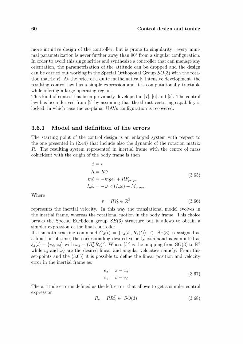
Table 3.6: Second formulation of integral backstepping, control parameters

α1 7α2 12λΦ 8α3 7α4 12λΘ 8α5 10α6 13λΦ 5

If the dynamics of p, q, r from (3.18) are substituted in (3.62) the moments canbe extracted and the resulting control takes the form:LM

N

= E

[K1Eα +K2eα +K3eα

]−[EE−1 +Dstab

]pqr

−G (3.63)

With

Dstab =

∂L∂p 0 0

0 ∂M∂q

0

0 0 ∂N∂r

G =

I−1xx

[(Iyy − Izz)qr

I−1yy

[(Izz − Ixx)pr

I−1zz

[(Ixx − Iyy)pq

. (3.64)

It can be noticed that the structure of the control variable is consistent with whatcan be expected from a control law that takes into account the rotation betweenbody and inertial frame: the control action computed in inertial reference frameis mapped in body frame while the gyroscopic effects and the stability derivativesare directly compensated.The H∞ tuning technique has not been adopted for the tuning of this control sincethe high nonlinearities introduced makes it ineffective. In this case the parameterhave been chosen via subsequent refinements trying to get the best result. Thechosen values are shown in Table 3.6.This kind of control, even if it is mathematically more adherent to the nonlinear

quadrotor model, nevertheless is subject to the limitations imposed by the Eulerangles parametrization, thus it is infeasible when Θ = ±90. In order to avoid thesingularities intrinsic in the angle parametrization a geometric control architecturehas been studied, both for the position and the attitude control.

3.6 Geometric control

In the previous developments the Euler angle parametrization of the special or-thogonal group has been extensively adopted. This parametrization allows a


more intuitive design of the controller, but is prone to singularity: every mini-mal parametrization is never further away than 90 from a singular configuration.In order to avoid this singularities and synthesize a controller that can manage anyorientation, the parametrization of the attitude can be dropped and the designcan be carried out working in the Special Orthogonal Group SO(3) with the rota-tion matrix R. At the price of a quite mathematically intensive development, theresulting control law has a simple expression and it is computationally tractablewhile offering a large operating region..This kind of control has been previously developed in [7], [6] and [5]. The controllaw has been derived from [5] by assuming that the thrust vectoring capability islocked, in which case the co-planar UAVs configuration is recovered.

3.6.1 Model and definition of the errors

The starting point of the control design is an enlarged system with respect tothe one presented in (2.44) that include also the dynamic of the rotation matrixR. The resulting system represented in inertial frame with the centre of masscoincident with the origin of the body frame is then

x = v

R = Rω

mv = −mge3 +RFprops

Inω = −ω × (Inω) +Mprops.

(3.65)

Wherev = RVb ∈ R3 (3.66)

represents the inertial velocity. In this way the translational model evolves inthe inertial frame, whereas the rotational motion in the body frame. This choicebreaks the Special Euclidean group SE(3) structure but it allows to obtain asimpler expression of the final controller.If a smooth tracking command Gd(t) =

(xd(t), Rd(t)

)∈ SE(3) is assigned as

a function of time, the corresponding desired velocity command is computed asξd(t) =

(vd, ωd

)with ωd = (RT

d Rd)∨. Where [.]∨ is the mapping from SO(3) to R3

while vd and ωd are the desired linear and angular velocities namely. From thisset-points and the (3.65) it is possible to define the linear position and velocityerror in the inertial frame as:

ex = x− xdev = v − vd

(3.67)

The attitude error is defined as the left error, that allows to get a simpler controlexpression

Re = RRTd ∈ SO(3) (3.68)


This expression of the left attitude error represents the transport map τl that isused to compare the desired tangent vector Rd in the tangent space of the currentorientation, that is:

R− τl(Rd

)= R−ReRd = R(ω − ωd) (3.69)

and the expression of the left velocity error is straightforwardly derived as

eω = ω − ωd (3.70)

Since the desired angular velocity ωd in the non-tilting quadrotor case is directlycomputed by the controller and not imposed by the user, from now on it will bereferred as ωc, keeping the notation used in [5] . For the same reason, also Rd isdenoted as Rc from now on , since only the yaw angle can be set. Finally, thenavigation error function Ψ has been defined as

Ψ =1

2

(KR(I −Re)

)KR = diag(kR1, kR2, kR3)

(3.71)

And the left trivialised derivative of Ψ can be expressed as

T ∗I LRe(dReΨ) = skew(KRRe)∨ = eR. (3.72)

Once the attitude tracking errors are defined, it is possible to set up a controlarchitecture for the position and attitude dynamics.

3.6.2 Control law

The position control law computes the forces along each axis in order to reachthe desired position. Of course in the non-titling UAV case, the force can beonly directed in the opposite direction of the z body axis e3. The main idea isto exploit the fully actuated rotational motion in order to orient the thrust axisdirection along the direction of the force required to track the position trajectory.This is the only feasible approach due to the inherent underactuation of co-planarplatforms [9]. Therefore, it is not possible to follow a decoupled attitude andposition motion but only the rotation around the third body axis can be freelyassigned, as shown next. In formulas

fc = c(Ψ)||fdc ||e3

fdc = −Kxex −Kvev −mge3 +mvd

c(Ψ) =ΨMax −Ψ

ΨMax

(3.73)

Where Kx, Kv are diagonal matrices to be tuned and a feed-forward compensationof the weight and inertial forces can be noticed. c(Ψ) is a weighting function for


the required control action, it is equal to one when the quardotor is correctlyoriented and thus the thrust generated by the propellers pushes the UAV in thecorrect direction, while when the orientation is different from the desired one, theattitude control is preferred and so the thrust is scaled in order to increase theposition error pushing the quadrotor along a wrong direction.Once defined the desired force, it can also be computed a desired attitude in orderto have the thrust directed in the right direction: the z body axis has to be in thesame direction of the desired force, while the x and y ones should be consistentlyoriented in order to get the desired yaw angle ψd. The Rc matrix is then built upassembling all the column vectors created from these requirements:

bd =

cosψdsinψd

0

(3.74)

Rc =[bc1 bc2 bc3

](3.75)

bc3 =fdc||fdc ||

(3.76)

bc2 =bc3 × bd||bc3 × bd||

(3.77)

bc1 = bc2 × bc3 (3.78)

The desired orientation of the UAV can be fed to an attitude controller inorder to compute the required control torques.It is possible to consider the attitude control law as a PD controller plus somefeed-forward terms, since the proportional action is included in the computationof eR [2]

τc = −RTc eR −Kωeω + Inωc + ωc × (Inω). (3.79)

In this case the feed-forward terms have a not-negligible weight and have to becomputed in real time by the controller since the matrix Rc is computed on board.As stated before

ωc = (RTc Rc)

∨

ωc = (RTc Rc − ωc)∨

(3.80)

so the first and second derivative of the computed desired attitude have to beworked out

Rc =[bc1 bc2 bc3

]. (3.81)

The three columns are the derivatives of the previously defined vectors and so ananalytical expression for each of them can be obtained by derivation. The firstterm to be computed is the third column as before, where the effect of the control


action affects the value of the derived vector

bc3 =fdc||fdc ||

− (fd,Tc × fdc )fdc||fdc ||3

fdc =KxKv

mex +

(K2v

m−Kx

)ev −

Kv

mDf +mvd

Df = Rfc − fdc

(3.82)

From the third vector the second column can be computed recalling (3.77)

bc2 =c

||c||− (cT × c) c

||c||3

c = bc3 × bdc = bc3 × bd + bc3 × bd

bd =

−ψd sinψdψd cosψd

0

(3.83)

and as last step deriving (3.78)

bc1 = bc2 × bc3 + bc2 × bc3. (3.84)

The second derivative of the rotation matrix is used for the computation of theinertial effects compensation and its the mathematical development follows thesame step just shown

Rc =[bc1 bc2 bc3

](3.85)

bc3 =fdc||fdc ||

− 2(fd,Tc fdc )fdc||fdc ||3

− (||fdc ||2 + (fd,Tc fdc ))fdc||fdc ||3

+ 3(fd,Tc fdc )2 fdc||fdc ||5

(3.86)

bc2 =c

||c||− 2(cT c)

c

||c||3+ 3(cT c)2 c

||c||5(3.87)

bc1 = bc2 × bc3 + 2(bc2 × bc3) + bc2 × bc3. (3.88)

Where

fdc =KxKv

mev +

(K2v

m−Kx

)(− Kx

mex −

Kv

mev +

Df

m

)− Kv

mDf (3.89)

Df = c(Ψ)Re(eω)∧fdc + c(Ψ)Re(Rceω)∧fdc − eRRceω

ΨMax

Refdc + c(Ψ)Ref

dc − fdc

(3.90)

c = bc3 × bd + 2(bc3 × bd) + bc3 × bd (3.91)

(3.92)


Table 3.7: Position control parameters, geometric control law

Kx Ky Kz Kv,x Kv,y Kv,z

3 3 3 2 2 2

Table 3.8: Attitude control parameters, geometric control law

KR1 KR2 KR3 Kw1 Kw2 Kw3

1 1 1 0.1 0.1 0.1

Using this control approach it is also possible to compute and an estimate for theregion of attraction of the equilibrium (ex, ev, Re, eω) = (0, 0, I, 0), see [5].The tuning of this control law has been tackled manually by a trial and errorprocedure because it has been impossible to set an optimization problem like theones seen before. For the sake of simplicity, the diagonal terms of each controlparameters matrix have been assumed to be equal and the resulting control tuningis shown in Tables 3.7, 3.8 setting the maximum value of Ψmax = 20.

Chapter 4

Simulation results

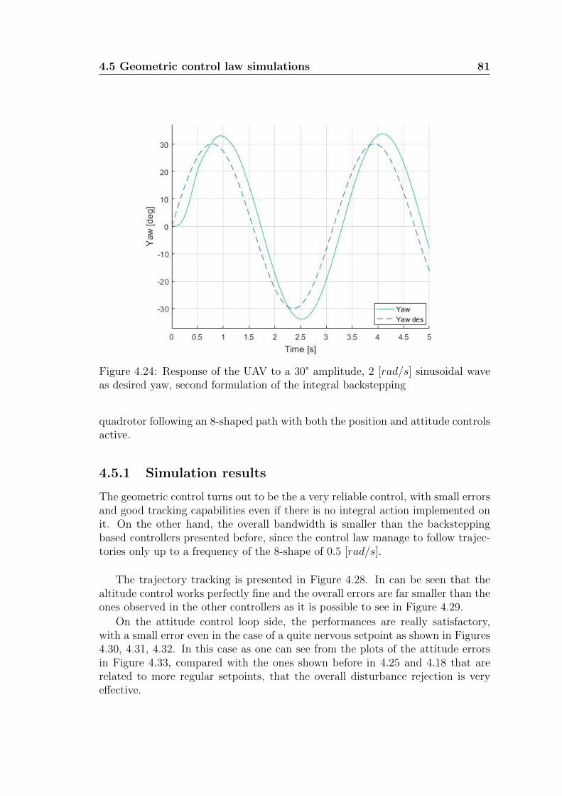
In this chapter the simulated results obtained using the previously developed non-linear control laws are presented.A first introduction to the Simulink simulator built in the FLYART laboratory isprovided at the beginning. Then all the presented control laws are tested.Each simulation campaign consists in a test on the attitude loop only and thenin the cascade of the attitude control with the position control. A comparisonbetween the results of the different architectures is proposed that highlights theresults achieved by each control law.Since it is not possible to define a cutting frequency for a nonlinear system, theattitude control tracking capabilities have been tested on a step response in firstissue and then on a sinusoidal setpoint.In a similar way, the position tracking has been validated using an 8-shape tra-jectory.

4.1 UAV simulator

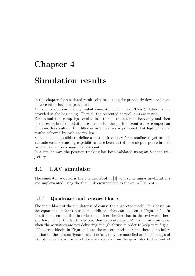
The simulator adopted is the one described in [4] with some minor modificationsand implemented using the Simulink environment as shown in Figure 4.1.

4.1.1 Quadrotor and sensors blocks

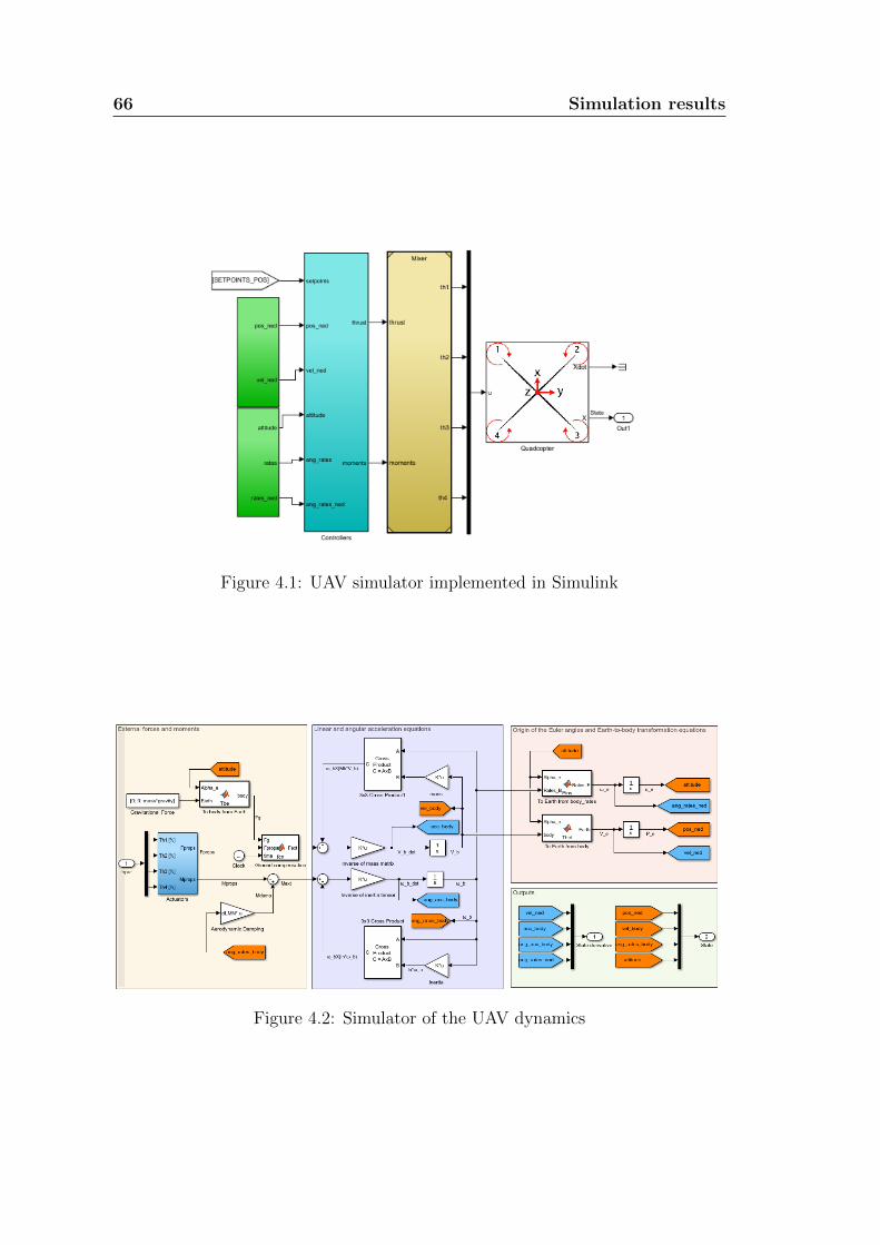
The main block of the simulator is of course the quadrotor model. It is based onthe equations of (2.44) plus some additions that can be seen in Figure 4.2 . Infact it has been modified in order to consider the fact that in the real world thereis a lower limit, the Earth surface, that prevents the UAV to fall at time zero,when the actuators are not delivering enough thrust in order to keep it in flight.

The green blocks in Figure 4.1 are the sensors models. Since there is no infor-mation on the sensors dynamics and noises, they are modelled as simple delays of0.01[s] in the transmission of the state signals from the quadrotor to the control

66 Simulation results

Figure 4.1: UAV simulator implemented in Simulink

Figure 4.2: Simulator of the UAV dynamics

4.1 UAV simulator 67

system.The measured signals are sent to the controllers that computes the required thrustand moments in order to follow the desired trajectory. These control signals aresent to the Mixer that inverting the relation derived in (2.37) computes the de-sired angular rates for the actuators.

4.1.2 Actuators model

The brushless DC motors dynamics has been identified in [4].It forces a limit on the performance of the control system and have to be consideredboth in tuning and in validation phases. The identified model is a first order lowpass filter that relates the throttle computed by the FCU using the mixer and theobtained rotational speed. The transfer function is then

G(s) =Ω(s)

Th(s)=

5.2

1 + s(92× 10−3). (4.1)

In Figure 4.3 it is possible to see that the actuators bandwidth is approximatelyequal to 55.5[rad/s].

Figure 4.3: Bode magnitude plot of the frequency response of the actuators trans-fer function


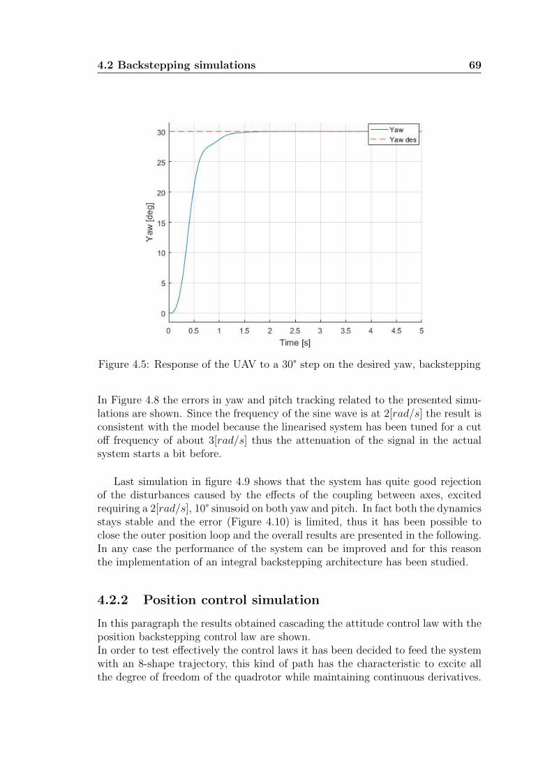
4.2 Backstepping simulations

4.2.1 Attitude control simulation

The simulations for the attitude control law have been carried out closing theattitude loop only. In order to do this a constant thrust of magnitude equal tothe UAV weight has been imposed to the actuators and the controller has beenin charge of the required moments computation.The result of the first simulation in shown in Figure 4.4 , a step of 30 on thepitch angle has been required while roll and yaw desired values are set to zero. Itis possible to see that the system reaches 90% of the desired value in about 0.5[s]and then to the final value in about 1[s]. This result is consistent with the tuningsince the required bandwidth for the system was in the range (0.48-1.1)Hz.The same simulation settings can be used to test the yaw control law. The relatedresults are proposed in Figure 4.5 and the resulting dynamic is slower than thepitch one since the inertia around the Z axis is bigger than the other two.

Figure 4.4: Response of the UAV to a 30° step on the desired pitch, backstepping

A second simulation campaign has been carried out applying a sinusoidal in-put with 30 amplitude at 2[rad/s] frequency.In Figures 4.6 and 4.7 it is possible to see the response of the system. It is clearthat there is a delay of about 0.2[sec] that strongly affects the performance of thesystem due to the delay in sensors and the dynamics of the actuators.

4.2 Backstepping simulations 69

Figure 4.5: Response of the UAV to a 30° step on the desired yaw, backstepping

In Figure 4.8 the errors in yaw and pitch tracking related to the presented simu-lations are shown. Since the frequency of the sine wave is at 2[rad/s] the result isconsistent with the model because the linearised system has been tuned for a cutoff frequency of about 3[rad/s] thus the attenuation of the signal in the actualsystem starts a bit before.

Last simulation in figure 4.9 shows that the system has quite good rejectionof the disturbances caused by the effects of the coupling between axes, excitedrequiring a 2[rad/s], 10° sinusoid on both yaw and pitch. In fact both the dynamicsstays stable and the error (Figure 4.10) is limited, thus it has been possible toclose the outer position loop and the overall results are presented in the following.In any case the performance of the system can be improved and for this reasonthe implementation of an integral backstepping architecture has been studied.

4.2.2 Position control simulation

In this paragraph the results obtained cascading the attitude control law with theposition backstepping control law are shown.In order to test effectively the control laws it has been decided to feed the systemwith an 8-shape trajectory, this kind of path has the characteristic to excite allthe degree of freedom of the quadrotor while maintaining continuous derivatives.


Figure 4.6: Response of the UAV to a 30° sinusoidal variation of the pitch setpointat 2 [rad/s], backstepping

Figure 4.7: Response of the UAV to a 30° sinusoidal variation of the yaw setpointat 2 [rad/s], backstepping

4.2 Backstepping simulations 71

Figure 4.8: Pitch and yaw tracking errors, backstepping

Figure 4.9: Attitude response on a sinusoidal reference on both pitch and yaw,backstepping


Figure 4.10: Attitude error on a sinusoidal reference on both pitch and yaw,backstepping

In figure 4.11 it is possible to see the response on the x, y axes with a frequencyof the 8-shape equal to 1.35 [rad/s] . On those axes the results are clearly satis-factory, with small overshoots and an almost perfect tracking.

Some different considerations can be done regarding the behaviour of the zaxis dynamics in Figure 4.12.

It can be noticed that the response is quite noisy, this fact is due to the factthat the required rate of the 8-trajectory push the quadrotor to its limits.Nonetheless the control works fine as it can be seen from the plot of trackingerrors in Figure 4.13.

4.3 Integral backstepping simulations

4.3.1 Attitude control law simulation

The integral backstepping control law has been developed in order to gain therobustness properties given by the integral action and to bring the steady stateerror to zero.From Figure 4.14 the improvement on the step response performances of aboutone tenth of second can be noticed.

On the other hand the gain in robustness and the zero steady state error makes

4.3 Integral backstepping simulations 73

Figure 4.11: Response of the x, y coordinate to an 8-shape trajectory, backstep-ping

Figure 4.12: Response of the z coordinate to an 8-shape trajectory, backstepping


Figure 4.13: Tracking error of the response to an 8-shape trajectory, backstepping

Figure 4.14: Response of the UAV to a 30 step on the desired pitch, integralbackstepping

4.3 Integral backstepping simulations 75

the yaw control more aggressive once tuned with the H∞ causing an overshoot onthe step response as can be seen in Figure 4.15 This sensibility of the system tostep inputs suggests the choice of feeding the system with smooth setpoints.The overshoot shown is anyway fully acceptable for the system under control sincea 30 step on any coordinate is to consider aggressive and unlikely to happen.

Figure 4.15: Response of the UAV to a 30° step on the desired yaw, integralbackstepping

The responses to sinusoidal inputs of 30° amplitude at 2[rad/s] on the pitchand yaw setpoints are shown in Figure 4.16, 4.17. Consistently with the adoptedtuning, the bandwidth of the linearised system is around 5 [rad/s] and thus theresulting response is slightly damped. As for the step response, the yaw control lawresults to be quite aggressive. However, as said before, it is completely acceptable.

Analysing the behaviour of the error due to the sinusoidal input in Figure 4.18,it can be seen that the improved speed of the response and the gained robustnesshave as counterpart a significant increment of the error.

4.3.2 Position control law simulation

An 8-shape at 1.35 [rad/s] has been fed to the system as setpoint in order toget a some comparable results between the pure backstepping control law and


Figure 4.16: Response of the UAV to a sinusoid of amplitude 30° on the desiredpitch at 2[rad/s], integral backstepping

Figure 4.17: Response of the UAV to a sinusoid of amplitude 30° on the desiredyaw at 2[rad/s], integral backstepping

4.4 Simulations of integral backstepping second formulation 77

Figure 4.18: Pitch and yaw tracking errors due to a sinusoid of amplitude 30° at2[rad/s] respectively on pitch and yaw, integral backstepping

the integral backstepping one. Figure 4.19 shows the obtained results and it ispossible to see comparing the errors shown in Figure 4.20 with the one in 4.13 thatthe altitude error has been reduced. This is possible because the disturbance onthe attitude can be ascribed to the effect of the coupling between the yaw and theother attitude coordinates, thus a better control action on the attitude improvesalso the performances of the position control loop.

4.4 Simulations of integral backstepping second

formulation

4.4.1 Attitude control law simulation

The response to a step on pitch and yaw setpoints is quite satisfactory as one cansee in Figure 4.21, 4.22. The system has a slower response than the other seenbut it has been considered acceptable since the improvement got on the positioncontrol.

The response to a sinusoidal reference shown in Figures 4.23, 4.24 is on thecontrary way better than the one obtained with the integral backstepping, with areduction of the attitude error up to 40% as it can be noticed from Figure 4.25.This fact is a clear example of the possibilities of this control law to improve the


Figure 4.19: Position of the UAV quadrotor during an 8-shaped trajectory at1.35 [rad/s], integral backstepping

Figure 4.20: Tracking error of the response to an 8-shape trajectory, integralbackstepping

4.4 Simulations of integral backstepping second formulation 79

Figure 4.21: Response of the UAV to a 30° step on the desired pitch,secondformulation of the integral backstepping

Figure 4.22: Response of the UAV to a 30° step on the desired yaw, secondformulation of the integral backstepping


behaviour of the overall system.

Figure 4.23: Response of the UAV to a 30° amplitude, 2 [rad/s] sinusoidal waveas desired pitch, second formulation of the integral backstepping

4.4.2 Position control law simulation

The better performances of the attitude control affects also the position trackingperformances. In Figure 4.26 the results of the simulation of an 8-shaped tra-jectory. While the overshoots are present like in all other simulations results, inthis case the overall performances are better than in the previous controllers asit can be expected from this more complex control law. This is clear looking atthe tracking errors plotted in Figure 4.27 where a better tracking on both y andz axes can be noticed.

4.5 Geometric control law simulations

For the geometric control law simulations it has been decided not to split theposition and attitude control laws but to handle them as a whole system.This choice is mainly caused by the formulation of the control law that does notallows a clear distinction between an inner attitude control loop and an outerposition loop. For this reason the presented results refer to a simulation of the

4.5 Geometric control law simulations 81

Figure 4.24: Response of the UAV to a 30° amplitude, 2 [rad/s] sinusoidal waveas desired yaw, second formulation of the integral backstepping

quadrotor following an 8-shaped path with both the position and attitude controlsactive.

4.5.1 Simulation results

The geometric control turns out to be the a very reliable control, with small errorsand good tracking capabilities even if there is no integral action implemented onit. On the other hand, the overall bandwidth is smaller than the backsteppingbased controllers presented before, since the control law manage to follow trajec-tories only up to a frequency of the 8-shape of 0.5 [rad/s].

The trajectory tracking is presented in Figure 4.28. In can be seen that thealtitude control works perfectly fine and the overall errors are far smaller than theones observed in the other controllers as it is possible to see in Figure 4.29.

On the attitude control loop side, the performances are really satisfactory,with a small error even in the case of a quite nervous setpoint as shown in Figures4.30, 4.31, 4.32. In this case as one can see from the plots of the attitude errorsin Figure 4.33, compared with the ones shown before in 4.25 and 4.18 that arerelated to more regular setpoints, that the overall disturbance rejection is veryeffective.


Figure 4.25: Pitch and yaw tracking errors due to a sinusoid of amplitude 30°at 2[rad/s] respectively on pitch and yaw, second formulation of the integralbackstepping


Figure 4.26: Position of the UAV quadrotor during an 8-shaped trajectory at1.35 [rad/s], second formulation of the integral backstepping

Figure 4.27: Tracking error of the response to an 8-shape trajectory, second for-mulation of the integral backstepping


Figure 4.28: Position of the UAV quadrotor during an 8-shaped trajectory at0.5 [rad/s], geometric control

Figure 4.29: Tracking error of the response to an 8-shape trajectory, geometriccontrol


Figure 4.30: Tracking of a roll setpoint, geometric control

Figure 4.31: Tracking of a pitch setpoint, geometric control


Figure 4.32: Tracking of a yaw setpoint, geometric control

Figure 4.33: Attitude error, geometric control

4.6 Final considerations 87

4.6 Final considerations

In this chapter the results obtained simulating each control law has been presentedand analysed.From this results it is clear that there are still margins for the development of abetter tuning procedure that can achieve better performances in tracking capa-bilities both for the position and the attitude control laws.It turns out that the H∞ tuning technique in this case give consistent results interms of the setted bandwidth for the closed loop system, while it is clear thatthe overall tracking performances can be improved.Eventually the Lyapunov based controllers turns out to have good performanceseven if they are limited by the assumptions presented in the previous chapters,while the geometric control has the potential to get better results but has theproblem not to have a standard tuning procedure in order to choose the values ofthe parameters, resulting in a slower control.

Conclusions

In the presented work of thesis the design, implementation and simulation of fourdifferent nonlinear control laws for a quadcopter UAV has been presented. Thecontrollers synthesised have been tested in different simulations and the resultshave been compared in the last chapter.In detail, the mathematical development of the control laws has been extensivelyanalysed in order to give a complete overview of the adopted techniques.For the first two control laws the tuning method adopted has been particularlyemphasised in order to give a complete example of how the minimization of theH∞ norm of the sensitivity can be adopted also for particular nonlinear systems.Eventually, the obtained results have been analysed and compared in order tostress the capabilities and limits of each controller.The goal to obtain a control law that can manage complex trajectories has beenreached, with a controlled system that can afford to undertake quite fast manoeu-vrers.Moreover, one of the main difficulties faced in nonlinear control design has alwaysbeen the choice of the tunable parameters values, since their effects on the sys-tem performance are not always clear. Thus the adoption of a standard tuningtechnique in this field results is a remarkable improvement in the possibilities toobtain a better choice of the control parameters.Due to hardware problems, it has not been possible to test properly the developedcontrol on the real UAV platform to provide meaningful data to be analysed. Theimplementation on the quadrotor of this control laws is thus the main develop-ment that will be undertaken in the near future. This work is actually already inprogress and have highlighted some limitations of the simulator developed in thelaboratory in modelling the noises and disturbances that acts on the real system.Another field of development for this work is a refinement of the H∞ tuningprocedure, adopted in order to better cope with the nonlinearities of the tuningproblem. As can be noticed from the simulation results, it works satisfactorilybut results sometimes in too aggressive control actions. This is mainly due to thenonlinear correlation shown in Chapter 2 between the Lyapunov parameters andthe related gains of the linearised controller.One last possible development would be the reformulation of the geometric controlin order to get an integral action both on the position and the attitude control.

90 Conclusions

This because the lack of this terms strongly affects the performances on the realsystem due to unavoidable constant disturbances like bias on the propellers thrust.

Bibliography

[1] Samir Bouabdallah and Roland Siegwart. Backstepping and sliding-modetechniques applied to an indoor micro quadrotor. In Robotics and Automa-tion, 2005. ICRA 2005. Proceedings of the 2005 IEEE International Confer-ence on, pages 2247–2252. IEEE, 2005.

[2] Francesco Bullo and Richard M Murray. Tracking for fully actuated mechan-ical systems: a geometric framework. Automatica, 35(1):17–34, 1999.

[3] Matteo Ferronato. Identificazione e controllo della dinamica verticale di unelicottero quadrirotore. 2016.

[4] Mattia Giurato. Design, integration and control of a multirotor uav platform.2015.

[5] Davide Invernizzi and Marco Lovera. Geometric tracking control of thrustvectoring uavs. arXiv preprint arXiv:1703.06443, 2017.

[6] Taeyoung Lee, Melvin Leok, and N Harris McClamroch. Nonlinear robusttracking control of a quadrotor uav on se (3). Asian Journal of Control,15(2):391–408, 2013.

[7] Taeyoung Lee, Melvin Leoky, and N Harris McClamroch. Geometric trackingcontrol of a quadrotor uav on se (3). In Decision and Control (CDC), 201049th IEEE Conference on, pages 5420–5425. IEEE, 2010.

[8] Lalo Magni and Riccardo Scattolini. ADVANCED and MULTIVARIABLECONTROL. Pitagora Editrice Bologna, 2014.

[9] Robert Mahony, Vijay Kumar, and Peter Corke. Multirotor aerial vehicles.IEEE Robotics and Automation magazine, 20(32), 2012.

[10] Simone Panza. Hinfguide. https://flyart.gitlab.io/hinfguide/, 2017.

https://flyart.gitlab.io/hinfguide/

Date post:	14-Jun-2020
Category:	Documents
Upload:	others
View:	10 times
Download:	0 times

Nonlinear attitude and position control for a quadrotor UAV · Nonlinear attitude and position...

Documents