J. Fluid Mech. (1997), vol. 352, pp. 65–112. Printed in the United Kingdom c 1997 Cambridge University Press 65 Nonlinear dynamics and pattern formation in turbulent wake transition By RONALD D. HENDERSON Aeronautics and Applied Mathematics, California Institute of Technology, Pasadena, CA 91125, USA (Received 1 October 1996 and in revised form 17 July 1997) Results are reported on direct numerical simulations of transition from two- dimensional to three-dimensional states due to secondary instability in the wake of a circular cylinder. These calculations quantify the nonlinear response of the system to three-dimensional perturbations near threshold for the two separate linear instabilities of the wake: mode A and mode B. The objectives are to classify the nonlinear form of the bifurcation to mode A and mode B and to identify the conditions under which the wake evolves to periodic, quasi-periodic, or chaotic states with respect to changes in spanwise dimension and Reynolds number. The onset of mode A is shown to occur through a subcritical bifurcation that causes a reduction in the primary oscillation frequency of the wake at saturation. In contrast, the onset of mode B occurs through a supercritical bifurcation with no frequency shift near threshold. Simulations of the three-dimensional wake for fixed Reynolds number and increasing spanwise dimen- sion show that large systems evolve to a state of spatiotemporal chaos, and suggest that three-dimensionality in the wake leads to irregular states and fast transition to turbulence at Reynolds numbers just beyond the onset of the secondary instability. A key feature of these ‘turbulent’ states is the competition between self-excited, three- dimensional instability modes (global modes) in the mode A wavenumber band. These instability modes produce irregular spatiotemporal patterns and large-scale ‘spot-like’ disturbances in the wake during the breakdown of the regular mode A pattern. Simu- lations at higher Reynolds number show that long-wavelength interactions modulate fluctuating forces and cause variations in phase along the span of the cylinder that reduce the fluctuating amplitude of lift and drag. Results of both two-dimensional and three-dimensional simulations are presented for a range of Reynolds number from about 10 up to 1000. 1. Introduction A fascinating feature of non-equilibrium fluid systems is the formation and de- struction of spatial patterns. Pattern formation can be viewed as the signature of an underlying instability and often gives the initial clues to understanding the dynamics behind a complex system. Cross & Hohenberg (1992) give a comprehensive review of pattern formation in hydrodynamics, nonlinear optics, chemical and biological systems. To a large degree the dynamics of these diverse physical systems can be de- scribed using similar concepts: linear instabilities, nonlinear saturation, mechanisms for pattern selection, and so forth. Elements of pattern formation are used in the present study as a framework for examining the sequence of global instabilities that develop in the wake of an infinitely long circular cylinder as it makes the transition
Transcript
J. Fluid Mech. (1997), vol. 352, pp. 65–112. Printed in the United Kingdom
Nonlinear dynamics and pattern formation inturbulent wake transition
By R O N A L D D. H E N D E R S O NAeronautics and Applied Mathematics,
California Institute of Technology, Pasadena, CA 91125, USA
(Received 1 October 1996 and in revised form 17 July 1997)
Results are reported on direct numerical simulations of transition from two-dimensional to three-dimensional states due to secondary instability in the wake of acircular cylinder. These calculations quantify the nonlinear response of the system tothree-dimensional perturbations near threshold for the two separate linear instabilitiesof the wake: mode A and mode B. The objectives are to classify the nonlinear formof the bifurcation to mode A and mode B and to identify the conditions under whichthe wake evolves to periodic, quasi-periodic, or chaotic states with respect to changesin spanwise dimension and Reynolds number. The onset of mode A is shown to occurthrough a subcritical bifurcation that causes a reduction in the primary oscillationfrequency of the wake at saturation. In contrast, the onset of mode B occurs througha supercritical bifurcation with no frequency shift near threshold. Simulations of thethree-dimensional wake for fixed Reynolds number and increasing spanwise dimen-sion show that large systems evolve to a state of spatiotemporal chaos, and suggestthat three-dimensionality in the wake leads to irregular states and fast transition toturbulence at Reynolds numbers just beyond the onset of the secondary instability. Akey feature of these ‘turbulent’ states is the competition between self-excited, three-dimensional instability modes (global modes) in the mode A wavenumber band. Theseinstability modes produce irregular spatiotemporal patterns and large-scale ‘spot-like’disturbances in the wake during the breakdown of the regular mode A pattern. Simu-lations at higher Reynolds number show that long-wavelength interactions modulatefluctuating forces and cause variations in phase along the span of the cylinder thatreduce the fluctuating amplitude of lift and drag. Results of both two-dimensionaland three-dimensional simulations are presented for a range of Reynolds numberfrom about 10 up to 1000.
1. IntroductionA fascinating feature of non-equilibrium fluid systems is the formation and de-
struction of spatial patterns. Pattern formation can be viewed as the signature of anunderlying instability and often gives the initial clues to understanding the dynamicsbehind a complex system. Cross & Hohenberg (1992) give a comprehensive reviewof pattern formation in hydrodynamics, nonlinear optics, chemical and biologicalsystems. To a large degree the dynamics of these diverse physical systems can be de-scribed using similar concepts: linear instabilities, nonlinear saturation, mechanismsfor pattern selection, and so forth. Elements of pattern formation are used in thepresent study as a framework for examining the sequence of global instabilities thatdevelop in the wake of an infinitely long circular cylinder as it makes the transition
66 R. D. Henderson
from simple to chaotic dynamics with increasing Reynolds number. We can relatethe linear instabilities of the ideal system to specific flow patterns observed in thewake and show that competition between these instability modes explains much ofthe complex behaviour observed in experiment. In many ways this scenario does notdepend on details of the system geometry and should represent the development ofcomplex dynamics in a number of similar free shear flows. Much of the focus in thepresent work will be on pattern destruction and the process that leads to irregulardynamics and ‘turbulence’ in the wake.
The two-dimensional vortex street in the wake of a circular cylinder is one of themost famous examples of pattern formation in fluids. It is known to result from aglobal Hopf bifurcation of the steady flow (Jackson 1987; Mathis, Provansal & Boyer1987; Zebib 1987). This bifurcation (the primary instability) occurs when the regionof absolute instability in the near wake of the cylinder becomes sufficiently large.The basic pattern of two-dimensional vortex shedding dominates our conceptual viewof the wake behind most bluff bodies. In the case of a circular cylinder, remnantsof two-dimensional vortex shedding persist to extremely high Reynolds number andcan still be observed when the wake is fully turbulent. Obviously the flow becomesmore complex with increasing Reynolds number and the ideal two-dimensional vortexshedding pattern is disrupted by transition in the free shear layers in the near wakeand eventually by turbulent transition in the boundary layer on the surface of thecylinder. However, the onset of ‘turbulence’ in the wake is an intrinsically three-dimensional phenomenon that begins at a low Reynolds number with the absoluteinstability of the two-dimensional flow with respect to spanwise perturbations (thesecondary instability).
Recent experiments have revealed a rich variety of pattern formation associatedwith the secondary instability of the Karman vortex street and subsequent transitionto turbulence. Roshko (1954) first identified the transition range for flow past acircular cylinder as the range of Reynolds number where velocity fluctuations becomeirregular. Early flow visualization studies by Hama (1957) and Gerrard (1978) linkedthose fluctuations with the development of ‘waviness’ in the spanwise vortices andGerrard’s ubiquitous ‘fingers of dye.’ However, it was Williamson (1988) who showedwith great clarity the intricate structure of the three-dimensional cylinder wake in thetransition range. The basic patterns consist of two types of three-dimensional vortexshedding that occur in a particular sequence as the Reynolds number is increased.Following the nomenclature introduced by Williamson (1988), we shall refer to theseinstabilities as mode A and mode B vortex shedding. Each flow pattern is centredaround a different spanwise wavelength and is observed with different degrees ofregularity. Quantitative visualization studies of the near wake by Mansy et al . (1994),Wu et al . (1996) and Brede, Eckelmann & Rockwell (1996) established the variationof wavelength with Reynolds number and even provided some direct experimentalmeasurements of the three-dimensional vorticity field. At the same time, Meiberg& Lasheras (1988) showed that similar three-dimensional shedding modes developnaturally from perturbations in the plane wake behind a splitter plate, so there isgood evidence that these phenomena represent instabilities in a broad family of freeshear flows.
The origin of these patterns in the wake of an infinitely long cylinder may beunderstood by examining the linear instabilities of the ideal two-dimensional flow(Noack & Eckelmann 1994; Barkley & Henderson 1996). Like the onset of vortexshedding, the relevant instabilities are global and absolute, and tied to the instabilityof three-dimensional global modes in the wake. Huerre & Monkewitz (1990) discuss
Pattern formation in wake transition 67
6
4
2
0150 200 250 300
Mode B
Mode A
k′2
k2
Re ′2
Re2
Re
k=
2p/b
Figure 1. Curves of neutral stability for the two-dimensional Karman vortex street with respect tospanwise perturbations. Linearly unstable modes exist everywhere inside the shaded regions. Theupper region corresponds to a family of long-wavelength instabilities with critical values Re2 ' 190,λ2 ' 3.96d; the lower region corresponds to a family of short-wavelength instabilities with criticalvalues Re′2 ' 260, λ′2 ' 0.822d. Each point (•) on this plot represents a three-dimensional modeconsidered in §3.
these relatively new and somewhat controversial stability concepts in the contextof spatially developing flows. The linear stability problem determines the structureand spatiotemporal symmetry of the global modes and the critical Reynolds numberwhere they first become unstable to small perturbations. Once perturbed these modesare self-excited and cause transition to a three-dimensional state. The symmetryof the three-dimensional wake after transition is determined by the spatiotemporalsymmetry of the destabilizing global mode. Barkley & Henderson (1996) showed thatthe three-dimensional flow patterns observed in experiment are due to two separatelinear instabilities, and that each instability leads to a distinct symmetry-breakingbifurcation from the ideal two-dimensional flow.
Figure 1 shows the neutral-stability curves for the wake, identifying the regionsof instability that produce modes A and B. Parameters characterizing the wakeinstability are the Reynolds number Re and the spanwise perturbation wavelengthλ (in units of cylinder diameter d) or wavenumber β = 2π/λ. For mode A thecritical values are Re2 ' 190 and λ2 ' 3.96d, while for mode B they are Re′2 ' 260and λ′2 ' 0.822d. There is now excellent agreement between computations based onthe the linear theory and experimental measurements of the critical wavelength andReynolds number (Barkley & Henderson 1996; Williamson 1996a–c). There is alsogood experimental validation of the symmetry of the destabilizing modes predictedby the linear theory (Barkley & Henderson 1996; Brede et al . 1996; Williamson1996b). Simulations of the three-dimensional flow by Zhang et al . (1995), Thompson,Hourigan & Sheridan (1996), and Henderson & Barkley (1996) have reproducedthe essential features observed in experiment and there is little doubt regarding thequalitative structure of the three-dimensional wake in the transition range.
What is not well understood is the scenario by which the wake develops irregulardynamics when the Reynolds number is increased beyond the secondary instabilitythreshold. In order to look at possible scenarios leading to ‘turbulence’ in the cylinder
68 R. D. Henderson
wake, we will put aside for the moment the ideal problem of flow past an infinitely longcylinder in an unbounded domain and consider only systems with a finite spanwisedimension L. In computation L represents the distance over which the velocity fieldis perfectly periodic (the size of the largest disturbances in the infinite system). Inexperiment Lmay be thought of as roughly analogous to the aspect ratio of the system,but end effects introduce a fundamental and important difference. We also make animportant conceptual assumption: that the dynamics may be described purely in termsof the global modes of the wake. This reduces the complexity of the three-dimensionalwake to a one-dimensional system, the only important dimension represented by thecharacter of the flow in the spanwise direction. Changes in the system dynamicscan be characterized with respect to two numbers: the control parameter Re (theReynolds number), and the system size L (the spanwise dimension). Experiments andcomputations show that for certain values of these parameters the flow has chaoticstates, that is irregular behaviour that persists to long times even under constantexternal conditions. This is a manifestation of instability in a deterministic systemand not of external noise. Chaotic behaviour is associated with systems that possessa large number of degrees of freedom which are excited as we go to the large-systemlimit Re → ∞, L → ∞. There are different possibilities depending on how we takethese limits.
In the idealized problem one should study the transition from regular to chaoticdynamics by taking L = ∞ and looking at the sequence of bifurcations that occur withincreasing control parameter Re. This is effectively impossible for computation unlesswe linearize about certain intermediate states. It is impossible in experiment althoughL can in principle be taken sufficiently large that finite-size and end effects are small.†In a more realistic scenario we can reach chaotic states in two ways, starting froma system with a sufficiently complicated set of linear instabilities. The simplest isto fix the control parameter Re and let L → ∞. In many situations this leads tospatiotemporal chaos characterized by the interaction of a moderate number of modesin a dissipative system. Alternatively, we can fix the system size L and let Re → ∞.This is the regime of strong turbulence achieved by removing all dissipation fromthe system. To talk about the ‘route to turbulence’ in the wake we must distinguishbetween these two limits.
The present study focuses not so much on the limiting values of these parametersas on how they affect the transition to irregular states observed in experiment. Directnumerical simulation (DNS) is used to study three-dimensional flows that arise fromperturbations to the two-dimensional wake in two ways: either for fixed L and smallvariations in control parameter Re, or for fixed control parameter Re and increasingsystem size L. In the latter case we follow the rationale given in §2.2, increasing theoriginal system size in powers of 2 in order to demonstrate changes in the dynamicsdue to the presence of more global modes, i.e. as we approach the continuousspectrum of the infinite problem. This particular sequence guarantees nested solutionspaces where the dynamics of smaller systems are embedded within those of largerones. Resolution is increased in proportion to L to ensure that the largest discretewavenumbers always lie in the dissipative part of the spectrum.
The neutral-stability diagram shown in figure 1 provides the necessary framework
† Finite-size effects are due to discretization of the continuous spectrum because of finite L,whereas end effects are due to the constant forcing of low-wavenumber modes by fluctuations at theends of a finite-span cylinder. Generally speaking, computations are restricted by finite-size effectsand experiments are polluted by end effects.
Pattern formation in wake transition 69
for reducing a study of the entire (Re, L)-parameter space to a small number offocused questions. There are three important cases to understand in relation totransition. First is the nonlinear response of the system to perturbations near thecritical point for mode A at Re2 (§3.3). In addition to providing the basic nonlinearform of the bifurcation, this also provides some qualitative information about allmodes in the A-band. Likewise, the second important case is the nonlinear responseof the system to perturbations near the critical point for mode B at Re′2 (§3.4). Thedynamics are special near these critical points since nonlinearity locks the flow intoa single symmetry-related mode. Finally, we look at how the wake responds awayfrom these critical points when a variety of three-dimensional modes are excited(§§3.5 and 3.6). In spite of the seeming complexity of the three-dimensional flowduring transition, these calculations show that the dynamics are controlled by a smallnumber of self-excited global modes in the wake. In each case the growth of thesemodes can be related to the formation of specific flow patterns during transition.We shall also see that nonlinearity leads directly to irregular states throughout thetransition range, rather than through a sequence of further bifurcations. In a morequalitative sense, the simulations show the effect of large-scale structure in the wakeon fluctuating forces and flow patterns at higher Reynolds number.
2. Computational methods2.1. Formulation
We consider the motion of a viscous fluid past an infinitely long circular cylinderplaced perpendicular to a uniform free stream. The fluid is assumed to have constantdensity ρ and constant dynamic viscosity µ. The idealized incompressible flow dependson three dimensional parameters: the cylinder diameter d, the free-stream speedu∞, and the kinematic viscosity of the fluid ν = µ/ρ. The only non-dimensionalcombination of these parameters is defined as the Reynolds number, Re ≡ u∞d/ν,and this serves as the control parameter for the system. The problem may be describedin dimensionless variables with u∞ and d serving as the reference scales for velocityand distance. The state of the fluid at any time t as it moves past the cylinder isdetermined by the velocity field u(x, y, z, t) and the pressure field p(x, y, z, t). Thesefields are described in a coordinate system where x is aligned with the freestreamdirection, y is normal to the free stream, and z is along the span of the cylinder.
Our main objective is to determine the nature of the flow dynamics as a functionof Re. The evolution of the flow is described by the incompressible Navier–Stokesequations, written in non-dimensional form as
∂u
∂t= −N (u)− 1
ρ∇p+
1
Re∇2u in Ω, (2.1a)
∇ · u = 0 in Ω. (2.1b)
N (u) represents the nonlinear advection term:
N (u) ≡ (u · ∇)u. (2.1c)
The computational domain Ω represents a region of three-dimensional space sur-rounding the cylinder that contains what is deemed to be the ‘important’ part of theflow.
The first step of the discretization is to reduce the problem on infinity to a problemon a domain of finite spanwise dimension L. In other words, we consider only those
70 R. D. Henderson
flows u(x, t) that satisfy the periodicity requirement
u(x, y, z, t) = u(x, y, z + L, t).
This is an important restriction on the solution space for moderate L and someimplications are discussed below. The three-dimensional spatially periodic field u canbe projected exactly onto a set of two-dimensional Fourier modes uq as
uq(x, y, t) = L−1
∫ L
0
u(x, y, z, t)e−i(2π/L)qz dz.
Likewise, the spanwise modes uq give the expansion of the velocity field in a Fourierseries:
u(x, y, z, t) =
∞∑q=−∞
uq(x, y, t)ei(2π/L)qz.
Substituting the Fourier expansion of the velocity field into the Navier–Stokes equa-tions, we obtain a coupled set of equations for the Fourier modes. To simplifythe notation, we define the scaled wavenumber βq ≡ (2π/L)q and the q-dependentoperators
∇ ≡ (∂x, ∂y, iβq), ∇2 ≡ (∂2x, ∂
2y,−β2
q ).
The evolution equation for the Fourier modes can then be written as
∂uq∂t
= −N q(u)−1
ρ∇pq +
1
Re∇2uq in Ω, (2.2a)
∇ · uq = 0 in Ω. (2.2b)
The nonlinear advection term provides the coupling between all modes. We candenote this term by
N q(u) = L−1
∫ L
0
N (u)e−i(2π/L)qz dz. (2.2c)
Dissipation becomes important at wavenumbers βD ∼ Re1/2; at wavenumbers β > βDthe equations are dominated by viscosity. These high-wavenumber modes contributelittle to the dynamics of the flow at large scales because their energy is rapidlydissipated by viscosity. For an adequate description of the dynamics in a systemwith a given spanwise dimension L we only need a finite set of M Fourier modes tocover the range of scales from β = 0 (the mean flow) to βD = (2π/L)M ∼ Re1/2, or
M = O(LRe1/2). We take as our final representation of the velocity field the truncatedexpansion
u(x, y, z, t) =
M∑q=−M
uq(x, y, t)ei(2π/L)qz.
Equations (2.1) and (2.2) are simply alternative ways to describe the flow. Com-putationally it is more convenient to follow the evolution of the two-dimensionalFourier modes uq(x, y, t) than the full three-dimensional field u(x, t). Because u isreal, the Fourier modes satisfy the symmetry u−q = −u∗q . Therefore, only half of thespectrum (q > 0) is needed. In addition to convenience, the Fourier representation ofthe velocity field has other intrinsic advantages. It provides a direct way of linkingparticular modes of the system with specific three-dimensional spatial patterns. Linearstability theory can predict which modes will have the strongest interaction with the
Pattern formation in wake transition 71
two-dimensional flow to produce these patterns. The time-averaged amplitude of theFourier modes gives a direct indication of how well-resolved the calculations are. Andfinally, the time-dependent amplitude of the Fourier modes provides a convenient wayof explaining the transfer of energy to different scales in the three-dimensional wake.
2.2. Subspaces and the approach to infinity
Although our goal is to study the flow past an infinitely long cylinder, this isclearly not possible in a simulation of the full Navier–Stokes equations. Periodicboundary conditions are often used in computational fluid dynamics to approximatethe flow on an infinite domain, but this is a false assumption. Periodic boundaryconditions do not reproduce the same dynamics unless the dimension of the systemin the periodic direction is large enough to provide a good representation of thecontinuous spectrum of the infinite problem. Keep in mind that the only admissiblewavelengths are those which are consistent with the boundary conditions: λq = L/q.Even ‘random noise’ introduced in a computation with periodic boundary conditionscan only excite a discrete set of modes with these wavelengths. Choosing L toosmall can exclude important instability modes altogether or it can simply excludethe modal interaction that leads to complex behaviour in large systems. Here wesuggest a rationale for exploring the dynamics of the infinite problem by examiningthe dynamics in a particular sequence of successively larger systems with carefullychosen initial conditions.
We begin by considering the effect of periodic boundary conditions on the spaceof possible solutions. For a given periodic length L, the velocity field u lies within asubspace spanned by the Fourier modes uq . We can write this as follows:
u(x, y, z, t) ∈ SL = spanuq(x, y, t)e
i(2π/L)qz, q = 0,±1, . . .. (2.3)
The Navier–Stokes equations preserve this subspace, meaning that the state whichevolves from an initial condition in SL will always remain there – the flow itselfcannot generate larger scales. Because of the Fourier expansion of the velocity field,a sequence of larger subspaces can be nested in the sense that
SL ⊂ S2nL ⊂ S∞. (2.4)
This means that every mode uq in SL is also a mode of S2nL, so that as we increaseL in powers of 2 we are adding new degrees of freedom while retaining all degreesof freedom of the smaller systems. As long as we follow this sequence, the final statein each small system lies within an exact (stable or unstable) subspace of all largersystems. This is the most precise way to study the approach to the dynamics of theinfinite problem.
Fluctuations at the ends of a finite-span cylinder in experiments set the scaleof the largest disturbances and provide a sustained excitation at low wavenumbers.Nonlinearity guarantees that all modes will be excited to some degree. The situation isquite different in computation. In the light of (2.3) we may adopt the computationalpoint of view that a spanwise-periodic perturbation at wavelength λ defines theeffective spanwise dimension (L ≡ λ) because there is no mechanism within theNavier–Stokes equations to generate larger scales. The initial conditions are thecritical factor rather than the imposed periodic boundary conditions. From (2.4) wecan see that the same initial condition will evolve to the same final state in the infinitesystem because the flow u(x, t) always remains within the finite-dimensional subspaceSL. The resulting spatially periodic flow may be a valid solution to the Navier–Stokes equations in an ‘infinite’ domain, but it is physically irrelevant unless we can
72 R. D. Henderson
mesh K Li Lo d/2Li
M1 148 to 170 8 24 0.0625M2 166 to 175 16 32 0.03125M3 182 to 201 32 48 0.015625
Table 1. Domain size parameters for the small, medium, and large computational domains shownin figure 2. The factor d/2Li is the blockage (fraction of the cross-sectional area 2LiL obstructed bythe cylinder area dL).
also show it is stable in the presence of longer wavelength disturbances, i.e. in eachlarger subspace. The present study will show that, for fixed Reynolds number, ‘small’systems (L ≈ 1d) give rise to time-periodic behaviour while ‘large’ systems (L ≈ 10d)evolve to a state of spatiotemporal chaos. Because the dynamics are controlled bythe interaction of a small number of instability modes, computations with moderateL are sufficient for deducing what happens in the limit L→∞.
2.3. Implementation
The fully discrete solution relies on the representation of the Fourier modes, uq(x, y, t)and pq(x, y, t), by a non-conforming spectral element method. The formulation fornon-conforming elements was introduced by Bernardi et al . (1992) as an extensionto the original spectral element method developed by Patera (1984). In the spectralelement method the computational domain is partitioned into K non-overlappingelements, and within each element both the solution and geometry are representedby a high-order polynomial basis. In two or more dimensions this basis can beconstructed as a product of one-dimensional polynomials. The current implementa-tion uses curvilinear quadrilateral elements and relies exclusively on Gauss–LobattoLegendre polynomials to represent the discrete solution. Any two-dimensional fieldis described by KN2 numbers, where N is the number of basis coefficients in eachdirection. Since the complex vector field uq(x, y, t) has six scalar components (threereal and three imaginary), it requires 6 × KN2 numbers. The full three-dimensionalvector field u(x, t) is expanded over 2M + 1 such modes, but because of the symme-try of these modes the discrete representation only requires a total of 6 ×MKN2
coefficients. Likewise, the pressure field p(x, t) is described by 2×MKN2 coefficients.The number ndof ' 2×MKN2 is equivalent to the number of grid points in physicalspace needed to represent all degrees of freedom in a three-dimensional scalar field.In the present set of calculations, ndof ≈ 106 grid points.
Figure 2 shows the basic computational domains used for simulations of thewake over the entire range of Reynolds number and table 1 shows the domainsize parameters. The formulation described above can be used for two-dimensionalsimulations by solving only for the zeroth Fourier mode. Simulations of the three-dimensional flow use the same computational domain for all Fourier modes. Althoughthe Fourier modes could alternatively be discretized by introducing a finite differencegrid or a collection of finite elements, the non-conforming method used here allowsfor local mesh refinement while preserving the block structure of the calculations.The computational domains shown in figure 2 represent only the base mesh andcalculations at various Reynolds numbers incorporate some refinement of the nearwake. The use of a non-conforming mesh to simulate the flow at lower Reynoldsnumber is helpful but not critical. Beyond the details of the polynomial basis and thetreatment of non-conforming elements in the mesh, the method follows a standard
Pattern formation in wake transition 73
M1
M2
M3
L
Li Lo
Figure 2. Computational domains used in the present study. Each domain is a subset of thelargest. The parameters Lo and Li determine the cross-sectional size, and L determines the spanwisedimension. Each computational domain is divided into K elements, and within each element thesolution and geometry are represented by N2 polynomial coefficients. The three-dimensional flow isdecomposed into M Fourier modes in the periodic spanwise direction.
Galerkin finite element procedure to discretize equation (2.2). Further details of thisparticular approach for non-conforming elements are described by Henderson &Karniadakis (1995).
Boundary conditions are required for the velocity and pressure fields on all exteriorboundaries of Ω, including the surface of the cylinder. For convenience these arespecified in physical rather than Fourier space. At the surface of the cylinder the fluidvelocity satisfies the no-slip condition: u(x, t) = (0, 0, 0). Far away from the cylinderand outside the wake, it matches the free-stream velocity: u(x, t) = (1, 0, 0). Across theoutflow plane downstream the approximate boundary condition for the velocity fieldis ∂x u(x, t) = (0, 0, 0). At this same location the pressure is set to a constant valueof zero. Along all other boundaries the pressure satisfies the high-order Neumannboundary condition given by Karniadakis, Israeli & Orszag (1991). This condition,which is derived by requiring the pressure field to satisfy the normal component of themomentum equation along the boundary, helps control divergence errors introducedby the splitting scheme described below.
The location of external boundaries affects quantities derived from the simulations
74 R. D. Henderson
such as shedding frequency and drag. The detailed convergence study presentedby Barkley & Henderson (1996) was used as the principal guide in selecting anappropriate size and resolution. The smallest domain, M1, is somewhat larger thandomains used in similar calculations of the three-dimensional flow over this range ofReynolds number (Karniadakis & Triantafyllou 1992; Zhang et al . 1995; Thompsonet al . 1996). Even this domain produces an acceptable quantitative simulation of theflow. In order to reduce the blockage effect on M1 the constant-velocity boundaryconditions were replaced with a condition of periodicity for both velocity and pressurealong the upper and lower boundaries of the wake region, i.e. u(x, y − Li, z, t) =u(x, y + Li, z, t) for x > 0. Results for all three domains agree to better than 2%. Theeffect of spanwise dimension L is examined directly in §3.
The set of modal equations are integrated forward in time using the three-stepsplitting scheme described by Karniadakis et al . (1991). This time-stepping algorithmreplaces equation (2.2) by a sequence of steps where the nonlinear terms are computedexplicitly while the pressure and diffusion terms are treated implicitly. Each implicitstep requires the solution of an elliptic boundary-value problem as described below.The algorithm is essentially a projection method with a consistent pressure boundarycondition that yields (in practice) second-order time accuracy. The explicit treatmentof the nonlinear terms dictates the maximum allowable time step through a CFL-typecondition, (∆t/∆x)|u|max 6 const. ≈ 0.72. In all of the calculations |u|max = O(1),the minimum grid size is ∆x ≈ 0.007, and the corresponding maximum time step is∆t ≈ 0.005.
Discretizing the implicit part of the time integration produces a set of linear systemsfor the discrete pressure and velocity fields that must be solved at each time step.Since both the real and imaginary parts of the complex pressure field satisfy the samealgebraic system of equations, there are only M systems to form (2M to solve). Thethree components of the velocity vector also satisfy the same system of equations,giving M additional systems to form (6M to solve). Each system is described by areal-valued matrix that is symmetric and positive-definite with a rank of O(KN2).Each matrix is reduced by factoring into Schur-complement form to eliminate rowsand columns associated with element interiors. This reduced system for the boundarypoints has a rank of O(KN) and can be solved directly from the LU factorizationof the Schur-complement matrix. Once the boundary solution is known, the solutionon the interior of each element can be updated by solving K smaller systems ofrank O(N2). The Schur-complement factorization is crucial for the direct solution ofthe large matrix systems associated with spectral element methods. Factorization isperformed once at the beginning of the calculation, and time stepping only requiresback-substitution using the stored matrices. The procedure is identical for each of theFourier modes and equivalent to solving 2M independent two-dimensional problemswith real data.
The repetition of calculations for each of the Fourier modes suggests a naturalstrategy for distributing the computational work over a collection of parallel pro-cessors: data for each mode is assigned to a different computer. Time integration iscarried out for each mode in parallel with an exchange of data at the beginning ofthe time step to evaluate the nonlinear term. This term is computed pseudo-spectrallyon a grid of points in physical space through use of the fast Fourier transform (FFT).The nonlinear calculation was not dealiased and although there is some pollution ofhigh-wavenumber modes this is not a problem at moderate Reynolds number. Duringthe FFT data are exchanged (the Fourier components) among all processors in thealgorithmic equivalent of a parallel matrix transpose. This communications kernel is
Pattern formation in wake transition 75
common to most parallel implementations of spectral methods (see e.g. Karniadakis& Orszag 1993). Evaluating the nonlinear term accounts for roughly one-quarter ofthe computational work. The remaining work goes toward solving the linear systemsin the pressure and diffusion steps. These calculations require no interaction betweenmodes and they proceed in parallel with the work perfectly balanced across thecollection of parallel processors.
The strategy outlined above was implemented on two dedicated parallel computers:the Intel Paragon and the Cray T3D. Both of these machines offer relatively fastcompute nodes and a custom communications network with low latency and highbandwidth. The data exchange needed to evaluate the nonlinear term was performedvia explicit message passing. The code communicates through a limited set of driversso that porting to new message passing systems is relatively easy, i.e. only newcommunication drivers need to be written. For example, after developing the code onthe Paragon, porting it to the T3D only took a few hours. The largest calculationsperformed as part of the current study involve 8×MKN2 ≈ 6 to 7 million unknownsper time step and 2 to 3 gigabytes worth of run-time data (field data and storedmatrices). Distributed over 64 processors, these calculations take approximately 5 sper time step on either machine. Simulations at this resolution would have beenimpractical without access to large-scale parallel computing systems.
3. Results3.1. Overview
The present study encompasses a wide range in Reynolds number from Re ≈ 10(steady two-dimensional flow) to Re = 1000 (turbulent three-dimensional flow). Webegin with an overview of changes in the flow dynamics with increasing Reynoldsnumber, concentrating on the response of wake oscillation frequency (shedding fre-quency) and mean drag coefficient. Both are unique functions of Reynolds numberalong the two-dimensional branch of solutions. From an ensemble of experimentalmeasurements, their values at low Reynolds number are currently known to withinan accuracy of about 5%, although the experimental shedding frequency curve in thetwo-dimensional range is now believed to be accurate to better than 1% (Williamson1996a). Both shedding frequency and drag show distinct changes at the various bi-furcation points of the wake and can be used as a guide to interpreting changes inthe wake structure and dynamics as a function of Reynolds number.
In non-dimensional form the shedding frequency is referred to as the Strouhalnumber. It is defined as St ≡ f d/u∞, where f is the peak oscillation frequency ofthe wake. Shedding frequency measurements in the laboratory are typically madeusing hot-wire signals from the unsteady velocity field near the edge of the separatingshear layer. However, because vortex shedding is associated with a global instability,any signal derived from measurements of the flow carries the signature of the vortexshedding frequency. Shedding frequencies presented here are generally determinedfrom the zero-crossing points of the unsteady lift signal. Shedding frequency can bemonitored as a direct indication that the unsteady flow is converging to a limit cycle.
The Strouhal–Reynolds number relationship is shown in figure 3. At low Reynoldsnumber the flow is steady (St = 0) and symmetric about the centreline of the wake.At Re1 ' 47 the steady flow becomes unstable and bifurcates to a two-dimensional,time-periodic flow. The shedding frequency of the two-dimensional flow increasessmoothly with Reynolds number along the curve shown in figure 3. Note that each
76 R. D. Henderson
0.1010 100 1000
2D
Re ′2=260
Re2=190
Re
Steady
0.15
0.20
0.25
Experimental fit
Re1= 47
St≡
fd/u
∞
Figure 3. Variation of wake oscillation frequency (Strouhal number) with Reynolds number forthe flow past a circular cylinder, from experimental measurements and computer simulations: ,Williamson (1989); •, Hammache & Gharib (1991); +, three-dimensional simulations from thepresent study; the solid line is a curve fit to two-dimensional simulation data for Re up to 1000.Dashed lines mark the critical Reynolds number for various wake instabilities. The shaded areaindicates a subcritical range described in §3.3 where the wake is unstable to finite-amplitudeperturbations.
point along the two-dimensional curve represents a perfectly time-periodic flow andthere is no evidence of further two-dimensional instabilities for Reynolds numbers upto Re ≈ 1000. At Re2 ' 190 the two-dimensional wake becomes absolutely unstableto long-wavelength spanwise perturbations and bifurcates to a three-dimensional flow(mode A). As the wake passes through the bifurcation point at Re2, experimentsindicate that there are two important changes in the shedding frequency: (i) there isa sharp drop in magnitude, and (ii) above Re2 the flow is no longer time-periodic butoscillates within a broad band of frequencies. Experimental frequency measurementsshown in figure 3 which are not along the two-dimensional branch represent thedominant peak in those broad-band spectra. There is a direct relationship betweenthe drop in frequency and the onset of mode A; we return to this point in §3.3. Theother feature of the frequency curve relevant to the present study is the change inslope at Re′2 ' 260 which coincides with the linear instability of mode B. Althoughmode B is observed in experiments at Reynolds number as low as Re ≈ 200, there isclearly a measurable change in shedding frequency at Re′2. Note that three-dimensionalcalculations follow the experimental trend for Re > Re2.
Figure 4 shows the drag curve for flow past a circular cylinder for Reynoldsnumbers up to 1000. In the computations the spanwise-averaged fluid force F (t) is
Pattern formation in wake transition 77
010 100 1000
2D
Re ′2
Re2
Re
Steady
1
2
3
Re1
CD
Figure 4. Drag coefficient as a function of Reynolds number for the flow past a circular cylin-der, from experimental measurements and computer simulations: (,•), Wieselsberger (1921); +,three-dimensional simulations from the present study; the solid line is a curve fit to two-dimensionalsimulation data for Re up to 1000.
computed by integrating the shear stress and pressure over the surface of the cylinder.The x-component of F is the drag, the y-component is the lift. The force is normalizedby the free-stream dynamic pressure and the projected area of the body to produceforce coefficients. The drag coefficient is defined as CD(t) ≡ Fx(t)/ 1
2ρu2∞dL. The mean
drag CD is simply the time-averaged value of CD(t). Because CD is determined froman average over the surface of the cylinder, it is much less sensitive to changes in thecharacter of the wake at low Reynolds number than single-point measurements likethe shedding frequency. The ‘textbook’ version of the drag curve is generally plottedon a log-log scale where the only discernible feature is the drag crisis at Re = O(105).The flat response of CD to changes in Reynolds number is compounded by the factthat experimental drag measurements are extremely difficult to make at low Reynoldsnumber, and subtle details of the drag curve are lost in the experimental scatter. Thedecrease in magnitude of CD in the steady regime can be fitted to a power-law curveand also makes a sharp but continuous transition at Re1. Henderson (1995) gives theform and coefficients for the steady and unsteady drag curves. At the onset of vortexshedding about 1/3 of the total drag force is due to skin friction from the boundarylayer and 2/3 is due to pressure drag. With increasing Reynolds number the skin-friction component continues to drop off while the pressure drag steadily increases. Athigher Reynolds number the drag is due almost entirely to the variation in pressurearound the surface of the cylinder. From Re1 to Re2 the drop in skin friction and
78 R. D. Henderson
increase in pressure drag almost cancel so that the CD–Re curve is relatively flat inthis range. Experiments do not indicate a substantial change in the drag curve at Re2
but there is a sharp drop away from the two-dimensional curve beginning at Re′2.Qualitatively, the drag and shedding frequency curves show similar behaviour but thechanges in CD are more subtle. Three-dimensional calculations also show a decreasein drag for Re > Re2, but there are not enough experimental measurements for adetailed comparison.
3.2. Nonlinear dynamics and ‘global modes’ of the wake
Everything that follows is based on the concept that spatially developing flows supportself-excited global modes. Common examples of such flows include wakes, jets, andshear layers. In the case of flow past a circular cylinder we can represent the three-dimensional flow near the secondary instability threshold as a combination of twoglobal modes. These modes represent the saturated primary instability (φ0) and asecondary instability mode (φ1):
u(x, t) = U(t)φ0(x, t) + A(t)φ1(x, t). (3.1)
φ0 and φ1 are assumed to be time-periodic functions with unit norm; U(t) andA(t) give their time-dependent amplitudes. In the linear approximation φ1 is simplythe leading eigenfunction of a temporal (Floquet) stability problem with given realwavenumber β and growth rate σ(β).† The local modes of the system would be theeigenfunctions of the one-dimensional Floquet stability problem associated with thetime-periodic base flow at a given streamwise location. All local modes with a givenβ are contained in the global mode for that β.
Our first goal is to understand the effect of small perturbations to the two-dimensional flow. By definition the primary instability φ0 is at a finite-amplitudeequilibrium state U(t) = U0. For |A| |U0| the amplitude of the secondary instabilityis given by A(t) ∝ exp σt, and φ1 takes the form
φ1(x, t) = φ1(x, y, t)eiβz + φ∗1(x, y, t)e
−iβz.
Now assume that the system responds such that σ(β) < 0 for Re < Rec and σ(β) = 0for Re = Rec, β = βc. We define the reduced control parameter ε ≡ (Re−Rec)/Rec tocharacterize small variations from the critical value Rec. For parameter values ε < 0the flow is linearly stable, whereas for ε = 0 there is a pattern-forming instability thatsets in at finite wavenumber β = βc. For ε > 0 the infinite system has a continuous bandof wavenumbers β− < βc < β+ for which the flow is unstable. Small perturbationsnear the critical point (Rec, βc) will result in a three-dimensional flow pattern thatgrows everywhere in space with a structure determined by φ1. Although we cannotwrite down an explicit form for φ1, we can identify the patterns formed due to itspresence in the flow. Linear theory is enough to predict the critical Reynolds number(Rec) and pattern wavelength (λc = 2π/βc), but nonlinear effects must be included ifwe want to understand the dynamics of the flow beyond the mere onset of the linearinstability.
A low-dimensional dynamical systems approach is a natural way to analyse globallyunstable flows. Close to a critical point we can reduce the dynamics of the three-dimensional wake to those of a discrete-time dynamical system. We take an approach
† In general σ will be complex, but Barkley & Henderson (1996) show that the most unstablemodes of the wake all have real σ. Here we interpret the complex frequency σ as a real (temporal)growth rate.
Pattern formation in wake transition 79
similar to the one above, fixing the perturbation wavelength λ = λc and writing thegrowth rate as σ = σ(ε). Next we discretize time by only examining the state of thesystem at discrete times tn representing one pass through the shedding cycle. Theglobal modes are time-periodic, φi(x, tn+1) = φi(x, tn), so the dynamics are describedlargely by the discrete-time evolution of their amplitudes, Un ≡ U(tn) and An ≡ A(tn).Our goal is to model the Navier–Stokes equations with a simple nonlinear equationfor these amplitudes.
As the instability grows the linear superposition (3.1) no longer holds. For |ε| 1 and |An| |U0| the flow can be represented as an expansion about the two-dimensional state in powers of the amplitude An. The form of that expansion may bededuced directly from the nonlinear form of the Navier–Stokes equations. Changesin the amplitude of φ0 as it transfers energy to φ1 are given by
Un = U0 −∞∑j=1
α0jA2jn . (3.2)
Near the linear instability the evolution of An will be given by An+1 = µ1An, whereµ1 = exp σTn is the discrete-time linear growth rate and Tn is the length of periodnumber n. Nonlinearity eventually arrests the exponential growth and the long-timeevolution of An is given by
An+1 =
(µ1 −
∞∑j=1
α1jA2jn
)An. (3.3)
Note that each of the constants µ1 and αij is some function of ε. Near the criticalpoint the variation of the linear growth rate is approximately µ1 = 1 + µ′1ε, whereµ′1 ≡ dµ1/dε. In this same regime the αij will be assumed constant since their variationsare O(ε2) or smaller. For a given initial state (U0, A0), the amplitude equationsdescribe the behaviour of transients (Un, An) and identify the finite-amplitude states(U∞, A∞) which the flow evolves to at long times. Experiments or simulations of thefull Navier–Stokes equations are needed to determine the values of the nonlinearcoefficients.
Nonlinear classification of the bifurcation (U0, 0) → (U∞, A∞) depends on the signof α11, also called the Landau constant. Positive α11 corresponds to a supercritical orsoft bifurcation. In this case the transition is continuous and the flow is stable belowthe critical point (ε < 0). Negative α11 signifies a subcritical or hard bifurcation. Inthis case the transition is discontinuous and hysteretic because the flow is unstableto finite-amplitude perturbations below the critical point (ε 6 0). To a large degreethe distinction depends on the value of the critical wavenumber βc relative to thedissipation range βD for the system. This classification can be made precisely bystudying the evolution of small perturbations with careful experiments or high-resolution computer simulations of the full nonlinear system.
In each of the calculations presented here we take initial conditions of the form (3.1).The mode φ0 is computed by integrating the two-dimensional Navier–Stokes equationsin a given domain until the flow converges to a limit cycle with amplitude U0. Fora given wavelength λ, the mode φ1 is set to the leading eigenmode of the temporalstability problem. The initial amplitude of φ1 is chosen so that |A0| ≈ 0.005|U0|, i.e. lessthan a 1% perturbation to the base flow. The evolution of the resulting (unstable) flowis then computed by integrating the full three-dimensional Navier–Stokes equations
80 R. D. Henderson
in a periodic domain capable of representing the initial perturbation and M of itshigher harmonics. The wavelength of the initial perturbation determines the spanwisedimension of the system, L = λ.
In the discrete nonlinear system the three-dimensional structure of the global modesis represented by a Fourier series expansion. Since φ0 ∝ u0 and φ1 ∝ u1, the amplitudeof a global mode at later times can be evaluated directly from the amplitude of itsfundamental Fourier mode:
|Un|2 =4
πd2u2∞
∫Ω
|u0(x, y, tn)|2 dΩ, (3.4a)
|An|2 =4
πd2u2∞
∫Ω
|u1(x, y, tn)|2 dΩ. (3.4b)
Although the full representation of φ1(x, t) involves higher harmonics for t > t0,nonlinearity locks these modes to the fundamental u1. Such modes are said to bepassive or slaved. In a pure bifurcation the fundamental mode carries the largestcomponent of the instability and is sufficient for tracking the amplitude. Note thatthe definition of amplitude in (3.4) depends on the computational domain Ω, andtherefore the nonlinear coefficients αij also depend on Ω. However, our primaryconcern is with the sign (positive or negative) of α11, and this is independent of howthe norm is defined.
3.3. Bifurcation to mode A: Re ' 190, L = 3.96d
Nonlinear calculations for the precise onset of the secondary instability were firstreported by Henderson & Barkley (1996). Some of those results are included herefor completeness. Figure 5 shows the growth and nonlinear saturation of a smallperturbation to the wake at Re = 195, λ = λ2 = 3.96d. The evolution of the three-dimensional flow was computed on the small domain M1 using M = 16 modes. AfterO(100) shedding periods the instability saturates. Near the point of saturation theinstability grows faster than the exponential growth described by An+1 = µ1An, whereµ1 ' 1.041 is the growth rate from linear stability calculations. Initially the correctionto the linear growth rate is given by µ1 − α11A
2n. Using the procedure described
by Henderson & Barkley (1996), the coefficient of this term may be estimateddirectly from the computational data as α11 ' −0.116. Negative α11 indicates that theinstability is subcritical.
Because the bifurcation to mode A is subcritical, the first two terms in (3.3) areinsufficient for determining the limiting amplitude. Assuming α12 > 0, the lowest-orderamplitude equation for the bifurcation to mode A becomes
An+1 = (µ1 − α11A2n − α12A
4n)An. (3.5a)
Substituting µ1 = 1 + µ′1ε, the equilibrium solutions to this equation for small ε are
|A|2 =|α11|2α12
±(α2
11
4α212
+µ′1ε
α12
)1/2
. (3.5b)
These amplitudes are shown as a bifurcation diagram in the inset to figure 5. Solidlines in the bifurcation diagram indicate stable states and dashed lines indicateunstable states. This diagram is necessarily schematic because the data do not permita reliable estimate of the coefficient α12. However, its value is clearly positive and
Pattern formation in wake transition 81
020 100
Re
An
0 40 60 80
Period number, n
180 200
0
1
|A|
An+1= (l1–α11 A2n) An
An+1=l1 An
0.2
0.4
0.6
0.8
1.0
1.2
Figure 5. Nonlinear growth of a three-dimensional perturbation to the wake near the secondaryinstability threshold at Re2 ' 190, λ2 = 3.96d: •, values of the amplitude An evaluated from simula-tions of the full Navier–Stokes equations at Re = 195; curves show predictions from equation (3.5)truncated at first and third order with µ1 = 1.041 and α11 = −0.116. The inset shows a bifurcationdiagram along with simulation results at nearby parameter values.
approximately equal to α12 ≈ 0.122. Additional calculations were performed at nearbyparameter values (see figure 1) to validate the predictions of finite-amplitude statesand the subcritical nature of the instability. At Re = 190 the flow was also foundto be subcritical with α11 ' −0.116. Below the critical point at Re = 185 the flowwas found to be bi-stable: initial conditions corresponding to A0 = 0.1 decayed backto zero, while initial conditions corresponding to A0 = 0.915 evolved to a saturatedthree-dimensional state with A∞ = 0.897. At Re = 180 the flow was found to be stableto finite-amplitude perturbations, providing a lower bound on the turning point andconfirming that the bifurcation diagram in figure 5 is approximately correct. Thereis clearly good agreement between the predictions of finite-amplitude states fromequation (3.5) and full nonlinear calculations for Reynolds numbers near the criticalpoint.
In addition to the finite-amplitude states that evolve from the linear instability,it is also interesting to look at how this bifurcation affects the global oscillationfrequency of the wake. Although values of tn are not evenly spaced in time, thephase of the oscillation corresponding to zero lift provides a reference for definingthe shedding period: CL(tn) ≡ 0. The distance between points tn changes smoothlyduring the transition to the new limit cycle and there is a well-defined instantaneousshedding period, Tn ≡ tn+1 − tn. We define the instantaneous shedding frequency asfn ≡ T−1
n . Simulations near the critical point suggest the following hypothesis: theglobal oscillation frequency is determined by the the primary instability mode φ0,
82 R. D. Henderson
20 100
Df0
0 40 60 80
Period number, n
fn – f0–0.01
0
0.01
–0.02
Un –U0
DU0
–0.1
0
Figure 6. Nonlinear frequency shift due to a perturbation at Re = 195, λ = λ2 = 3.96d (same timeseries as figure 5): , shift in global oscillation frequency (scale on the left); •, shift in amplitudeof the primary instability mode (scale on the right); the solid line is computed from equation (3.6)with parameter values γ01 = 0.01005, γ02 = 0.00740, and γ03 = −0.00517. The data verify that theglobal oscillation frequency follows the amplitude of the primary instability and explains the dropto the lower curve in figure 3.
and the oscillation of φ1 remains locked to this mode.† Since changes in φ0 arelargely characterized by changes in its amplitude, we can write fn = F(Un). Near thesecondary instability threshold F(Un) can be expanded in a Taylor series about itstwo-dimensional value, f0 = F(U0):
fn = F(Un) ≈ F(U0) +dF
dU(Un −U0)
= f0 − const.× α01A2n
= f0 − γ01A2n.
Higher-order corrections will involve an expansion in even powers of An, and thefrequency shift can be written in the same form as equation (3.2):
fn = f0 −∞∑j=1
γ0jA2jn . (3.6)
Like the coefficients α0j , the values of γ0j are ε-dependent with variations of O(ε2) orsmaller; they will also be assumed constant for |ε| 1.
The computed shift in global oscillation frequency fn due to the growth andsaturation of the mode A instability is shown in figure 6, with data which correspondto the same time series presented in figure 5. The change in amplitude of theprimary instability mode Un is overlayed with the frequency data, showing that thetwo are indeed of the same form. Equation (3.6) truncated at j = 3 with the givenparameter values reproduces the computed frequency shift almost exactly. This changein frequency during the bifurcation from the two-dimensional state to mode A vortexshedding accounts for the drop to the lower curve in figure 3. Because the bifurcationto mode A is subcritical, there is a discontinuous jump to the three-dimensional statewith a correspondingly large change in the amplitude of the primary and secondary
† One can also think of φ1 as a three-dimensional structure that wraps around thetwo-dimensional structure of φ0. It does not introduce a new time scale, but it can shift thetime scale of the primary instability.
Pattern formation in wake transition 83
instability modes. Since fn − f0 ∝ A2n, this jump is reflected by a large drop in the
global oscillation frequency of the wake.Perhaps the most interesting characterization of the state that exists after transition
is in terms of the three-dimensional structure of the flow. Figure 7 shows a visualizationof the fully saturated mode A state that evolves at Re = 195, just beyond the secondaryinstability threshold. Figure 7(a) shows isosurfaces of the three-dimensional vorticityfield, ξ ≡ ∇×u. The spatiotemporal symmetry of mode A (Barkley & Henderson 1996,equation (3.3)) produces a staggered array of streamwise vortices that alternate in signfrom period to period at a given spanwise location. Pattern formation in the systemis shown using normalized grey-scale images of the streamwise and normal velocitycomponents along the midplane of the wake. At saturation mode A produces asignificant distortion of the Karman vortex shedding pattern that gradually decreasesin amplitude with distance downstream from the cylinder. In the discrete-time systemthis is a stationary spatial pattern centred around the critical mode wavelengthλ = λ2 = 3.96d. The saturated state is perfectly time-periodic and the image shown isrepeated exactly from period to period. The pattern does not ‘wander’ along the spanor exhibit any other type of irregular behaviour. This spatially periodic flow patternrepresents an idealization of mode A observed in experiments near the secondaryinstability threshold (see e.g. Williamson 1988, 1991).
3.4. Bifurcation to mode B: Re ' 260, L = 0.822d
Next we consider perturbations to the wake near the short-wavelength instabilitythreshold at Re = 265, λ = λ′2 = 0.822d. The procedure is exactly the same, andthe evolution of the flow was also computed using M = 16 modes. Mode A doesnot appear owing to the restricted size of the domain. Figure 8 (see p. 86) showsthe results from this calculation. Starting from a small perturbation, the instabilitysaturates after O(50) shedding periods. The linear growth rate of the perturbation isµ1 ' 1.16. However, in this case the amplitude drops below the exponential growthcurve near saturation. The estimated value of the Landau constant for this bifurcationis α11 ' 3.92. Large positive α11 indicates that the instability is strongly supercritical.
Only two terms are needed to determine the limiting amplitude of a supercriticalinstability. The lowest-order amplitude equation for the bifurcation to mode B istherefore
Bn+1 = (µ1 − α11B2n)Bn. (3.7a)
For ε < 0 the flow always decays back to a two-dimensional state (B = 0), while forε > 0 there are finite-amplitude states given by
|B|2 = µ′1ε/α11. (3.7b)
These amplitudes are shown as a bifurcation diagram in the inset to figure 8. Thesupercritical nature of the bifurcation to mode B was verified by performing sim-ulations at nearby parameter values near the tip of the mode B instability region(see figure 1). Simulations at Re = 260 (just above the critical point at Re′2 = 259)and Re = 270 both evolved to three-dimensional states that lie near the predictedlimiting amplitude. Calculations below the critical point at Re = 255 decayed backto a two-dimensional state. Small perturbations at λ = λ′2 and smaller are stable forRe < Re′2.
One would not expect a large change in global oscillation frequency near the onsetof mode B for the following reason. A supercritical bifurcation represents a continuoustransition from the two-dimensional state. Any coupling to the primary instability
84 R. D. Henderson
(a)
êx= +0.75 (red), –0.75 (blue); |êz |=1 (silver)
Figure 7. (a). For caption see facing page.
(a)
êx= +0.5 (red), –0.5 (blue); |êz |=1 (silver)
Figure 9. (a). For caption see facing page.
mode is weak near onset because the bifurcating mode saturates at low amplitude|B|2 ∼ ε. For 0 < ε 1 both the global oscillation frequency and amplitude ofthe primary instability mode remain constant to O(ε) during the transition from thetwo-dimensional state to mode B. Although there will be a measurable change forsufficiently large ε > 0, the computations do not indicate any significant change in
Pattern formation in wake transition 85
(b)
u(x, y = 0, z, t) v(x, y = 0, z, t)
Figure 7. Visualization of mode A after transition at Re = 195: (a) isosurfaces of thethree-dimensional vorticity field; (b) spatial pattern formation in the velocity field, centred arounda spanwise wavelength of λ = λ2 = 3.96d. The image plane corresponds to x/d = (0, 24) andz/d = (0, 15.84), with a somewhat shorter downstream extent in image (a).
(b)
u(x, y = 0, z, t) v(x, y = 0, z, t)
Figure 9. Visualization of mode B after transition at Re = 265: (a) isosurfaces of thethree-dimensional vorticity field; (b) spatial pattern formation in the velocity field, centred arounda spanwise wavelength of λ = λ′2 = 0.822d. This flow pattern cannot be observed directly inexperiments because it is unstable to longer-wavelength modes in the A-band. The image planecorresponds to x/d = (0, 24) and z/d = (0, 13.12), with a somewhat shorter downstream extent inimage (a).
shedding frequency for Re ≈ Re′2 when the three-dimensional flow is restricted topure mode B.
Figure 9(a) shows the three-dimensional structure of the flow that evolves atRe = 265 as mode B develops in the wake. The spatiotemporal symmetry of mode B(Barkley & Henderson 1996, equation (3.4)) produces an inline array of streamwisevortices that have the same sign from period to period at a given spanwise location.This can also be interpreted as the symmetry of mode A plus a shift of the three-dimensional structure by half a wavelength after a time T/2. Figure 9(b) showsspatial pattern formation in the velocity field. To emphasize the relationship betweenthe long- and short-wavelength instabilities, this and subsequent flow visualizationin figures 11 and 13 are shown to the same scale. The nonlinear saturated stateproduces only a slight distortion of the basic two-dimensional flow with an amplitudethat decays rapidly with distance downstream of the cylinder. At moderate distancesdownstream there is no evidence of the mode B instability and the wake returns to atwo-dimensional state. As in the case of mode A, the saturated flow is time-periodic
86 R. D. Henderson
010
ReBn
0 30 40 50
Period number, n
240 280
0
|B |
Bn+1= l1 Bn
Bn+1= Bn×(l1–α11 B2n)
0.05
0.10
0.15
0.20
0.25
20
0.2
0.4
Figure 8. Nonlinear growth of a three-dimensional perturbation to the wake near the secondaryinstability threshold at Re′2 ' 260, λ′2 = 0.822d: •, values of the amplitude Bn evaluated from simula-tions of the full Navier–Stokes equations at Re = 265; curves show predictions from equation (3.7)truncated at first and third order with µ1 = 1.16 and α11 = 3.92. The inset shows a bifurcationdiagram along with simulation results at nearby parameter values.
and the spatial pattern is stationary. Although the flow pattern shown in figure 9 hassome qualitative similarities with mode B observed in experiment, this ‘pure’ statecannot be observed directly in the laboratory because the wake is absolutely unstableto mode A in this range of Reynolds number. We explore this issue in detail in thefollowing section.
3.5. Spatiotemporal chaos: Re ' 260, L→∞We now turn our attention away from the critical points to look at the dynamics ofthe wake in a sequence of systems with fixed control parameter Re and increasingspanwise dimension L. The sequence is computed at Re = 265 where both A-and B-type instabilities are self-excited (see figure 1). Note that the most-amplifiedmode A wavelength is not constant but decreases with Reynolds number (Barkley& Henderson 1996). At Re = 265 the ratio of the critical mode B wavelength to thefastest growing mode A instability falls close to a power of 2 (λ ' 3.288d = 4× λ′2)).Since this is not true at other values of the Reynolds number, Re = 265 is a uniquechoice for computing the sequence 2nL because the discrete spectrum includes thelargest eigenvalue in both the mode A and mode B instability regions. The results ofthe previous section constitute the first element of this sequence, i.e. the developmentof the flow in a system where the spanwise dimension is equal to the critical mode Bwavelength, L = λ′2 = 0.822d. Subsequent calculations are performed at four timesand sixteen times this length scale.
In analysing the complex flows that develop in these ‘large’ systems we will try to
Pattern formation in wake transition 87
synthesize the previous results for bifurcations to pure states, but the approach willbe slightly different. For moderate L there is a finite number of global modes thatparticipate in the dynamics. These modes are determined by the discrete wavenumbersthat fall into a region of instability in figure 1. An amplitude equation describingthe evolution of a single bifurcating mode near threshold does not directly apply.To interpret the process of nonlinear growth and saturation in a qualitative way wewill rely on flow visualization. In order to quantify how the three-dimensional flowdevelops we can follow the amount of kinetic energy Eq(t) carried by each Fouriermode during transition. The instantaneous kinetic energy at a given wavenumbermay be computed approximately as
Eq(t) =1
2ρ
∫Ω
|uq|2 dΩ. (3.8a)
The time-averaged kinetic energy over some interval (t0, t0 + T ) is given by
〈Eq〉 =1
T
∫ t0+T
t0
Eq(t) dt. (3.8b)
We refer to the variation of 〈Eq〉 with q as the spanwise energy spectrum. The spectrumis normalized so that 〈E0〉 = 1. Like the global mode amplitude defined in (3.4), thenumerical values of Eq(t) also depend on the region Ω where the integrals in (3.8) areevaluated. There is a direct link between the energy spectrum and flow visualization:a ‘spike’ in the spanwise energy spectrum corresponds to a spatial structure witha well-defined spanwise wavelength. This provides an analogy to the link betweenglobal mode amplitude and pattern formation near the critical points.
3.5.1. Quasi-periodic behaviour, L = 3.288d
The first case we consider is a system with spanwise dimension four times largerthan the critical mode B wavelength, L = 4 × 0.822d = 3.288d. The evolution ofthis flow was also computed using M = 16 modes since the highest wavenumbersstill lie within the viscous-dominated regime. The fundamental u1 with wavelengthλ = 3.288d corresponds to the most-amplified mode of the wake at Re = 265; thewavelength of the harmonic u4 lies just inside the tip of the mode B instabilityregion; all other wavelengths correspond to linearly stable modes. Since there aretwo self-excited instabilities in this system, we expect the dynamics to represent theinteraction of three global modes: φ0 ∝ u0, φ1 ∝ u1 (mode A), and φ2 ∝ u4 (mode B).Note that the full three-dimensional representation of φ1 and φ2 involves a sum overdifferent subsets of the Fourier modes uq , some of which carry shared componentsof the global modes. Although the fundamental mode for φ2 is a fourth harmonic ofφ1, the two global modes are decoupled due to the distinct spatiotemporal symmetryof modes A and B.
We start by looking at the shift in global oscillation frequency during the transitionto the three-dimensional state, shown in figure 10. Initially there is a large drop infrequency due to the growth and saturation of the mode A instability, followed by afast transition to a different state where the flow oscillates over a relatively narrowband of seven frequencies. Unlike the bifurcations to pure mode A or pure mode B,the asymptotic state is quasi-periodic with an oscillation period much longer thanthat of the two-dimensional flow. In this quasi-periodic state the average sheddingfrequency rises above the saturated mode A value and at times returns almost exactlyto the two-dimensional value f0. There are small variations in the flow during each
88 R. D. Henderson
20
Df0
0 40 60 80
Period number, n
–0.01
0
–0.02
2D
A
Figure 10. Shift in oscillation frequency during transition at Re = 265 for calculations on thedomain L = 3.288d. The asymptotic state is quasi-periodic and the wake oscillates within a groupof seven frequencies.
of the intermediate shedding cycles, but no attempt was made to characterize thevariations precisely.
These changes in oscillation frequency are linked to the spatial development ofthe flow. Figure 11 illustrates the structure of the wake as a series of patternsformed during transition. The entire sequence from initial perturbation to completesaturation takes O(50) shedding cycles. During this time the flow passes through twostates. The first coherent pattern emerges just as φ1 (mode A) saturates. This is thesame pattern associated with the critical mode at Re2 ' 190. All modes within themode A instability region produce this same basic pattern. As the amplitude of φ2
(mode B) grows the flow evolves to a second state identified by the appearance of theshort-wavelength mode B pattern in the near wake, superimposed over the larger-scale mode A pattern. Mode B appears later in time because it has a much smallergrowth rate. The state that exists at long times is a mix of both instability modes withan amplitude that depends on distance downstream of the cylinder. Notice that thehighly distorted mode A pattern in figure 11(a) becomes smoothed-out following theappearance of mode B in the near wake. The decrease in the amplitude of mode Acoincides with the rise of the global oscillation frequency in figure 10. This is thelink between figures 10 and 11: the growth of mode B causes a large reduction inthe amplitude of mode A, driving the system back towards a more ‘two-dimensional’state. We shall return to this point in §4.
3.5.2. Chaotic behaviour, L = 13.152d
Next we look at the development of the flow in a system where the spanwisedimension is sixteen times longer than the critical mode B wavelength, L = 16 ×0.822d = 13.152d. The evolution of the flow was computed using a total of M = 64modes on the same computational domain. The initial perturbation to u1 at thefundamental spanwise wavelength lies well outside the mode A instability region;the wavelengths of the first four harmonics u2−5 lie within the mode A instabilityregion; the wavelength of the harmonic u16 lies just inside the tip of the mode Binstability region (see figure 1). Note that the discrete-time linear growth rate ofthe first five modes is such that µ1 < 1 and µ2 < µ3 ≈ µ5 < µ4 (all greaterthan 1 and hence unstable). The system admits three incommensurate wavelengthsλi = ( 1
3, 1
4, 1
5) × L in the mode A instability region, plus one subharmonic of the
Pattern formation in wake transition 89
(b)
u(x, y = 0, z, t) v(x, y = 0, z, t)
(a)
(c)
Figure 11. Visualization of the three-dimensional flow that evolves from an initial perturbation atRe = 265, λ = 3.288d: (a) saturation of the most-amplified instability to give the mode A pattern;(b) the amplitude of mode A decreases as the mode B instability develops in the near wake; (c) theasymptotic state is a mix of both modes. The spanwise dimension L is only 1/4 of the image shown.
fastest-growing mode A instability. We expect the dynamics to be described by theinteraction of six global modes: the three modes of the previous section, plus threeadditional modes representing subdominant mode A instabilities. As before we canidentify each global mode with its corresponding fundamental Fourier mode: φ0 ∝ u0,φi ∝ ui+1 for i = 1 . . . 4 (mode A), and φ5 ∝ u16 (mode B).
As in the previous section we first look at the change in global oscillation frequency,shown in figure 12, as each of these instability modes develops in the wake. Initiallythe frequency drops as the most-amplified mode A instability grows, reaching aminimum value when the amplitude of this mode (φ3 ∝ u4) saturates. As before, thefrequency again rises rapidly when mode B settles into the near wake. However, atlong times the flow does not reach a periodic state. Instead it oscillates randomlywithin a narrow band of frequencies whose peak value is only slightly lower than thatof the two-dimensional flow. For the remainder of this section we will concentrate onthe bracketed region in figure 12 where the system makes a transition from regularto irregular dynamics.
The spatial development of the three-dimensional flow during this time is shownin figure 13. Similar to the transitional flow in the smaller system L = 3.288d,
90 R. D. Henderson
20
Df0
40 60 80
Period number, n
–0.01
0
–0.02
2D
A
(a) (b) (c) (d )
Mixed A–B
Figure 12. Shift in oscillation frequency during transition at Re = 265 from calculations on thelarge domain L = 13.152d. The asymptotic flow is chaotic and oscillates within a narrow bandof frequencies, slightly lower than that of the two-dimensional flow and centred around the levelmarked mixed A–B. Labels (a–d) refer to the flow visualization in figure 13.
the wake again passes through several states before reaching full saturation afterO(100) shedding periods. The first coherent pattern to emerge is identical to the oneshown in figure 11(a) and corresponds to saturation of the most-amplified mode Ainstability (φ3 ∝ u4). Again the wake does not saturate around this state becausesubdominant modes continue to grow. The state following saturation of the leadingmode is characterized by the appearance of irregular large-scale structures in thewake as shown in figure 13(b, c). These structures have remnants of mode A and arequalitatively similar to the ‘vortex dislocations’ reported by Williamson (1992). Theyare related to the growing amplitude of other self-excited mode A instabilities andlead to a breakdown of the regular mode A pattern. The state that exists at long times(figure 13(d)) does not exhibit any coherent large-scale structure. At long times theamplitude of all modes in the A-band equalizes to within an order of magnitude andthe dynamics are chaotic. Mode B appears in the near wake in the same qualitativeway as seen in figure 11(c): a small-scale pattern superimposed over the larger-scalestructure of the wake.
The primary distinction between the structure of the flow in this calculation and theresults for smaller systems is the development of these large-scale ‘turbulent’ structuresdue to the competition between multiple mode A instabilities. Figure 14 shows a close-up of the vorticity field just as mode A begins to break up. In the near wake thereis a complex intertwining of the mode A and mode B instabilities. This figure alsoreveals an isolated mode A vortex structure at the core of the ‘vortex dislocation’ infigure 13(b). Otherwise, the instantaneous vorticity field is highly complex and difficultto analyse directly. It should be intuitively clear from both figures 13 and 14 thatmode B dominates the near wake but quickly breaks up and is displaced by modeA slightly downstream. Also, compare the highly irregular state shown here with thepure mode B state shown in figure 9, keeping in mind that both flow fields correspondto Re = 265. Although mode B may appear to dominate the near wake, the effect ofmode A disturbances clearly makes a fundamental difference to the character of theflow at this Reynolds number.
The transition from regular to chaotic dynamics is quantified in figure 15. Thisfigure shows the instantaneous kinetic energy Eq(t) for roughly half of the spectrumfrom the initial saturation of the leading mode A instability until the flow reaches
Pattern formation in wake transition 91
(b)
u(x, y = 0, z, t) v(x, y = 0, z, t)
(a)
(c)
(d )
Figure 13. Visualization of the three-dimensional flow that evolves from an initial perturbationat Re = 265, λ = 13.152d: (a) saturation of the most-amplified instability around a wavelengthof λ = 3.288d to give the mode A pattern; (b,c) development of large-scale structure during thebreakdown of the mode A pattern; (d) asymptotic state with no discernible large-scale pattern. Theimages represent the full spanwise dimension of the system.
its asymptotic state. A set of labels is shown just above the t-axis so that the flowvisualization in figures 13 and 14 can be compared directly with the spanwise energyspectrum in figure 15. Each bold trace indicates the amplitude of one Fourier modeidentified as the fundamental mode for a self-excited global instability. The mostimportant feature of the time-dependent energy spectrum is the observation thatchaotic behaviour arises from the strong nonlinear interaction between the threeleading mode A instabilities, beginning at t− t0 ≈ 290.
We can clarify the interaction between secondary instability modes as follows.Whenever the flow admits two global modes φp and φq with fundamental wavenum-
92 R. D. Henderson
Figure 14. Visualization of the three-dimensional vorticity field during transition at Re = 265, justfollowing the breakdown of mode A and subsequent transition to a mixed A–B state. Only ξz = +1is plotted in order to reveal the streamwise vorticity in the near wake (ξx = ±0.65), since otherwiseit would be hidden by a sheet of negative spanwise vorticity shedding from the cylinder. Data forthis image is taken from figure 13(b).
bers βp and βq (not integer multiples), there is a redistribution of energy through thenonlinear term in the Navier–Stokes equations:
The first two terms on the right represent the self-interaction that links φp and φqback to the primary instability (β = 0) and to higher harmonics of their fundamentalwavenumbers. This is the only type of nonlinear interaction in systems that admita single secondary instability mode (§§3.3 and 3.4). Coupling between secondaryinstability modes is due to the last two terms on the right. These terms are responsiblefor both the forward cascade of energy to smaller scales,
N (φp + φq)ei(βp+βq) +N (φ∗p + φ∗q)e
−i(βp+βq), (3.10a)
and the inverse cascade of energy to larger scales,
N (φp + φ∗q)ei(βp−βq) +N (φ∗p + φq)e
−i(βp−βq). (3.10b)
This interaction drives global modes other than φp and φq . If there were no couplingbetween secondary instability modes we would expect the flow to saturate around thefastest-growing linear instability, producing a bifurcation to a pure three-dimensionalstate. Nonlinearity drives the amplitude of subdominant modes to a level far fromtheir equilibrium values and the flow never reaches a regular state. In figure 15 this isled by the triad interaction between Fourier modes u3–u4–u5 which transfers energyto both u1 and u2, causing the amplitude of higher-wavenumber modes to grow. Theasymptotic state may be interpreted as a competition between multiple oscillators
Pattern formation in wake transition 93
(a) (b) (c) (d )
Strong nonlinear regime
250 300 350 400t– t0
10–12
10–10
10–8
10–6
10–4
10–2
u4
u3
u5
u2
u1
Eq(t)
Figure 15. Spatiotemporal chaos in the wake at Re = 265. Each trace corresponds to the energy ofa three-dimensional mode with a given spanwise wavenumber (approximately half of the spectrumis shown). Bold traces correspond to the four modes that lie within the mode A instability region.At t − t0 ≈ 290 the flow enters a strongly nonlinear regime where subdominant instability modesgrow rapidly. At t − t0 ≈ 320 large-scale turbulent structures appear in the wake, marking thebreakdown of the regular mode A pattern and subsequent transition to the chaotic state that existsat long times. Labels (a–d) refer to the flow visualization in figure 13.
represented by the self-excited global modes φi(x, t), each trying to reach a differentequilibrium amplitude but driven off-peak by nonlinearity in the system.
The equilibrium amplitude that is reached by each mode in the fully couplednonlinear system is characterized by the time-averaged form of the spanwise energyspectrum, shown in figure 16. The spanwise energy spectrum indicates the averagedistribution of energy in the three-dimensional wake. Figure 16 shows results from allcalculations at Re = 265. For the (time-periodic) flows in small systems the averagingis performed over the time scale for which the flow is periodic, while for the (non-periodic) large system the averaging is performed over the time scale of figure 15.Following the ideas of Hohenberg & Shraiman (1989) we distinguish two basic lengthscales in the energy spectrum. The excitation length lE is the scale at which energy isextracted from the primary instability and injected into the three-dimensional flow.The dissipation length lD is the scale at which energy is dissipated by viscosity. Infigure 16 we identify lE primarily with the mode A instability because the energy levelin the mode B range is an order of magnitude lower. Based on the fact that mode Bis strongly supercritical, we can estimate lD as being somewhat smaller than thecritical mode B wavelength at Re = 265. At higher Reynolds number the excitation
Figure 16. Long-time spanwise energy spectrum of the three-dimensional wake after transition atRe = 265 for increasing system size: , L = 0.822d; ×, L = 3.288d; •, L = 13.152d. Shaded regionsindicate the approximate wavenumber bands affected by the mode A and mode B instabilities. Alsoindicated are the excitation scale lE due to mode A and the approximate dissipation scale lD dueto viscosity. The inset shows a portion of the data on a semilog scale to emphasize the connectionwith the primary instability at β = 0.
scale should remain approximately constant while the dissipation scale decreases aslD ∼ Re−1/2.
Low-wavenumber modes of the wake are linearly stable but essentially independentof viscosity (non-dissipative), and it is interesting that energy does not seem to falloff at low wavenumbers. While this result may seem odd at first, the reason is clearwhen the same data are plotted on a semilog scale as in the inset to figure 16. Theenergy spectrum is driven by the primary instability at β = 0, which in turn providesa sustained excitation through the secondary instability to a band of wavenumbersaround β ∼ l−1
E . Energy is redistributed to all modes by nonlinearity until the flowreaches a saturated state, but energy is only dissipated at wavenumbers larger thanβ ∼ l−1
D . At long times there is a continuous distribution of energy at all scales in thethree-dimensional wake, one of the essential features of a ‘turbulent’ flow.
We look at one other summary of the various calculations for Re = 265 byplotting the surface pressure distribution as a function of system size L. The surfacepressure coefficient is defined as Cp ≡ (p − p∞)/ 1
2ρu2∞, where p is the mean static
pressure on the surface of the cylinder. To convert from Cartesian to cylindricalcoordinates we take θ = tan−1 y/x so that θ = 0 is the base of the cylinder andθ = π is the front stagnation point. Figure 17 compares the surface pressure froma two-dimensional simulation with the results of three-dimensional calculations for
Pattern formation in wake transition 95
1
0
–1
–1.0 –0.5 0 0.5 1.0
–0.2 0 0.2–1.3
–0.2
–1.2
–1.1
–1.0A
A
B2D
h/p (rad)
Cp(h)
Figure 17. Surface pressure distribution for flow past a circular cylinder at Re = 265. This sequenceillustrates the effect of fixing the control parameter Re and increasing the system size L, starting froma simulation of the two-dimensional wake: curve B (L = 0.822d) only includes the short-wavelengthinstability; curve A (L = 3.288d) includes the effect of a single long-wavelength instability mode;curve A∗ (L = 13.152d) includes the effect of several long-wavelength modes and indicates thatCp(θ) has reached a level that is independent of system size L.
Re = 265 and increasing system size L. Note that Cp depends only on the componentof pressure exerted by the mean flow (β = 0) since all other Fourier componentshave zero contribution when averaged along the span of the cylinder. Small-scalethree-dimensionality alone (L = 0.822d) results in a relatively small reduction in themagnitude of Cp on the low-pressure side. This is because of the weak interactionbetween mode B and the primary instability near onset. The presence of mode A(L = 3.288d) causes a much greater reduction in the magnitude of Cp. Calculationsfor the largest domain (L = 13.152d) agree well with this curve and indicate that thecomputed surface pressure distribution has reached a level that is independent of thesystem size L.
Wake simulations at Re = 265 with L = 13.152d should represent all of theimportant qualities of the flow observed in larger experimental systems, excludingphenomena associated with end effects. In particular, larger systems at this Reynoldsnumber will also exhibit spatiotemporal chaos due to the same nonlinear mechanismdescribed above. Since this basic mechanism is in place for all Re > Re2, we expectthe calculations reported here for Re = 265 to represent the dynamics of the flow ina qualitative way for lower Reynolds numbers as well. This was verified directly atRe = 220 using a domain of spanwise dimension L = 14.78d and M = 64 modes. Thisdomain size was specifically chosen to include the most-amplified mode of the wakeat Re = 220 (λ ' 3.695d) and two subdominant mode A instabilities (see figure 1).In this system the flow also evolves to a state of spatiotemporal chaos at long times.Note that the chaotic states at Re = 220 and Re = 265 both involve a minimum of
96 R. D. Henderson
100 200
Df0
Period number, n
–0.02
0
0.02
–0.04
2D
150
A
Figure 18. Shift in oscillation frequency during transition at Re = 220 for calculations on thedomain L = 14.78d. The asymptotic flow is chaotic, but at this Reynolds number the frequencyremains low after transition because the amplitude of mode A remains large (see figure 3). Thespatial development of the flow in time is similar to the sequence shown in figure 13.
three incommensurate wavelengths in the mode A instability region. The evolution ofthe flow at Re = 220 is qualitatively similar to the wake structure shown in figure 13,including the appearance of large-scale disturbances just prior to the breakdown ofthe periodic mode A pattern. Figure 18 shows the shift in oscillation frequency andthe onset of spatiotemporal chaos following saturation of the linear instability. AtRe = 220 the (nonlinear) excitation of mode B is relatively weak so the amplitudeof mode A remains large. As a consequence the global oscillation frequency remainslow in the asymptotic state. This is consistent with experimental observations in thisrange of Reynolds number and the computed frequency shift agrees well with themeasured dominant frequency at Re = 220 shown in figure 3.
It is difficult to verify that the dynamics are chaotic at lower Reynolds number fromdirect numerical simulations of the full Navier–Stokes equations. Even the smallestsystem L that includes a few wavelengths in the mode A instability region becomesvery large as the width of the A-band shrinks near Re2. For example, at Re = 190 (justabove the critical point at Re2 = 188.5) the smallest system that includes three modesin the unstable mode A wavenumber band is L ≈ 75d, and M ≈ 300 modes would berequired to cover an appropriate range of scales. Intrinsically chaotic dynamics canstill be inferred from the broad-band frequency spectra observed in experiments; wereturn to this point in §4.
3.6. Simulations of the ‘turbulent’ wake: Re = 1000
The final set of calculations represent the flow far from the onset of the secondaryinstability, in the ‘fully turbulent’ regime at Re = 1000. The most comprehensivecalculations at this Reynolds number are performed on the large domain M3 witha spanwise dimension of up to L ≈ 25d. The number of Fourier modes required toreach the dissipation scale in this system can be estimated as βD = (2π/L)M ≈ Re1/2,or M ≈ 128 modes. At this resolution the calculations resolve the beginning of thedissipation range but not smaller scales, so the results must be considered somewhatqualitative. For example, there is a discrepancy of 10–20% between these calculationsand experimental measurements of the mean drag coefficient and base pressure (seefigures 4 and 21). However, the phenomena we wish to illustrate are related to thebehaviour of the wake at large scales and these modes are fully resolved. As in the
Pattern formation in wake transition 97
calculations at Re = 265, we follow a sequence of fixed control parameter Re andincreasing system size from L = 2πd ≈ 6.283d to L = 8πd ≈ 25.13d. The initialcondition for the first calculation is a perturbation to the two-dimensional flow atRe = 1000. Subsequent calculations are performed by taking the asymptotic flowon one domain and perturbing it at a lower wavenumber on a domain twice aslarge in the spanwise direction. The results illustrate some interesting pattern formingproperties of the system at large Reynolds number and the effect that large-scalethree-dimensionality in the wake has on the fluctuating forces and mean surfacepressure distribution.
Figure 19 shows a visualization of the unsteady flow at Re = 1000 on the largestdomain L = 8πd. The sequence of images is spaced approximately two sheddingcycles apart. The most striking feature is the spontaneous appearance of large-scalephase dislocations in the near wake. These are highly localized structures that differqualitatively from the large-scale structures associated with the breakdown of mode Aobserved at lower Reynolds number. The dislocations appear intermittently in timeand at random locations along the span. Various types of ‘dislocations’ or ‘defects’are a common feature in many pattern-forming systems. In most fluid systems wheredislocations have been studied experimentally, they are forced to occur by introducingsome controlled non-uniformity to avoid the inherent randomness in time and spaceof naturally occurring dislocations.
Based on time traces of the spanwise energy spectrum (not shown), the phasedislocations in figure 19 seem to be caused by the rapid accumulation of energy in thelow-wavenumber modes of the system. As the amplitude of these modes grows theshedding becomes out of phase over a distance equal to one-half their wavelength. Ifthe amplitude becomes large enough, a dislocation occurs with a complex reconnectionof vortices on either side. After the passage of a dislocation the wake is left in a‘winding state’ that still satisfies the periodic boundary conditions along the span.Additional dislocations at later times destroy the winding state and return the waketo a state of nearly parallel shedding. This cycle of events occurs repeatedly but ona slow time scale with new dislocations forming after O(10) shedding periods. Thephenomenon is not understood at a fundamental level and is reported here only as anobservation for this particular simulation. It is also unknown whether the irregularstate depicted in figure 19 will continue indefinitely or settle down to a more regularbut still ‘turbulent’ state after a long time.
The winding states observed in figure 19 are qualitatively similar to winding statesreported by Leweke & Provansal (1995) for the periodic wake of a ring at Re = O(100).Blackburn & Melbourne (1996) also show experimental evidence of winding statesand phase dislocations in the wake of straight circular cylinders at Reynolds numberas high as Re = O(105). Similar structures are observed in other types of free shearflows as well. Browand & Troutt (1980, 1985) showed that ‘vortex defects’ appearnaturally during transition in the mixing layer at the boundary between cells ofdifferent frequency, or between adjacent cells with the same frequency but a differentphase. Browand & Prost-Domasky (1990) studied these structures in a controlledsetting by acoustically forcing a shear layer at different frequencies along the span.In the wake simulations reported here the cylinder is perfectly uniform and there isno forcing. The only mechanism for generating dislocations is through the dynamicsof large-scale structures in the wake.
Large-scale three-dimensionality in the wake also has a pronounced effect on theunsteady forces exerted on the cylinder. Figure 20 compares the fluctuating lift anddrag for systems with increasing spanwise dimension L. These quantities are averaged
98 R. D. Henderson
(a)
(b)
(c)
(d)
(e)
( f )
(g)
(h)
Figure 19. Visualization of the turbulent wake at Re = 1000. The sequence of images (a–h) showscontours of the normal velocity v(x, y = 0, z, t) at times spaced approximately two shedding cyclesapart. The image plane corresponds to x/d = (0, 48) and z/d = (0, 25.13). The structures ‘wash out’downstream because of the low resolution in that part the domain.
along the span of the cylinder. Each trace is characterized by its time-averaged value(CL and CD) and the root-mean-square variation of the instantaneous value aroundthis average (C ′L and C ′D). The time-averaged lift coefficient is always zero. If thetwo-dimensional results were included in figure 20, the corresponding traces of CL(t)and CD(t) would both be perfectly time-periodic signals. Each three-dimensionalcalculation shows a varying degree of ‘irregularity’ that depends on the spanwisecorrelation of the flow. Because the signals are highly non-periodic it is difficult to
Pattern formation in wake transition 99
0 200 400 600 800
L=8pdL=4pdL=2pd
–2.0
–1.6
–1.2
–0.8
–0.8
–0.4
0
0.4
0.8
t
CL(t)
CD(t)
Figure 20. Unsteady lift and drag coefficients for the ‘turbulent’ flow past a cylinder at Re = 1000.The data illustrate the effect increasing domain size has on the fluctuating forces, up to the maximumof L = 8πd. The t-axis is only for scale: short gaps between data sets are long transients in thecomputations.
estimate the asymptotic values of the fluctuating forces without taking averages overextremely long times, but the qualitative effect of increasing L is quite clear.
In the smallest domain (L = 2πd) the shedding is well-correlated along the spanand the amplitude of the fluctuating lift and drag is quite large. The amplitude ofthe fluctuating component decreases with increasing L due to the loss of spanwisecorrelation. On the largest domain (L = 8πd) the force signals appear to be modu-lated, and there are times when the amplitude of the fluctuating lift falls almost tozero. Times of minimum C ′L(t) in figure 20 correspond to the appearance of phasedislocations in the wake. At these times the instantaneous force F (z, t) is misaligneddue to the phase difference and there is a certain amount of cancellation when theforce is averaged along the span. The time scale of the modulation is related to therise and fall of energy in the low-wavenumber modes of the system. The modulationis not periodic like the beating that would occur with a simple nonlinear interactionbetween two temporal frequencies, for example between the vortex shedding frequencyand the oscillation frequency of the separating shear layer. Instead the fluctuationsappear in bursts at irregular intervals, consistent with their origin as a feature of thecompetition between low-wavenumber spatial modes in the wake.
Another interesting effect of large-scale structure in the wake can be seen in thecomparison between instantaneous and time-averaged surface pressure distributions,shown in figure 21. This figure presents Cp(θ) at Re = 1000 obtained from bothexperimental measurements and simulations of the three-dimensional flow. First notethat the pressure distribution along the base of the cylinder is quite flat at thisReynolds number. This is also a direct result of weak spanwise correlation in a largesystem due to intrinsic three-dimensionality. The reduction in spanwise correlation
100 R. D. Henderson
1.00.50–0.5–1.0
–3
–2
–1
0
1
Cp(h)
h/p (rad)
Figure 21. Surface pressure distribution for flow past a circular cylinder at Re = 1000: (sym-bols), experimental measurements by Leyva, Henderson & Gharib (1996); the solid line is thetime-averaged pressure distribution from a three-dimensional simulation with L = 8πd; the dashedline is the potential flow solution. The ‘shaded’ region indicates the instantaneous values of Cp(θ, z, t)at 64 locations along the span.
results in a smoothing of the mean pressure distribution. A strongly correlated flowwould exhibit low-pressure peaks associated with the average position of vortexformation. For example, the surface pressure distribution at Re = 265 shown infigure 17 exhibits these peaks because the three-dimensional flow remains well-correlated along the span. The ‘shaded’ region in figure 21 reveals further evidence oflarge phase differences by showing the instantaneous cross-sectional surface pressurecoefficient Cp(θ, z, t) at 64 locations along the span. If the flow were well-correlated,this region would collapse into a narrow band (for the perfectly correlated two-dimensional flow it is a single line). Since the solid line indicates the mean value ofCp(θ), and the shaded area extends equally far above and below the mean value inthe base region, we can infer that at this instant there is a complete variation in phasealong the span of the cylinder.
When plotted as in figure 21 the difference between the computations and exper-imental measurements for the surface pressure coefficient does not seem that large.In the simulated wake the value of Cp at θ = 0 (the base pressure) is actually about10% more negative. This difference also accounts for the discrepancy in the com-puted drag coefficient shown in figure 4. Although the shape of the curve is in goodagreement with experiments, including the flatness of the base pressure region, thesurface pressure coefficients obtained from the computation are uniformly lower thanthe experimental measurements. This suggests that there is more dissipation withinthe boundary layer and near wake in the laboratory flow than in the simulated flow,which could arise from any number of sources: free-stream turbulence interactingwith the boundary layer, surface roughness, and so forth. It may also be due to a ne-
Pattern formation in wake transition 101
glect of small-scale three-dimensionality in the computational model. So far attemptsto isolate the discrepancy and close the gap between computation and experiment atthis Reynolds number have been unsuccessful.
4. DiscussionAt the present time there is still a vigorous debate over the precise physical
origin of the wake instability. Researchers have sought a more physical explanationof the two-dimensional vortex shedding instability for almost a century now, soimagine the difficulty of describing the more complicated three-dimensional instabilityin simple physical terms! Instead we focus primarily on how instability modes inthe wake determine the overall structure of the three-dimensional flow and thetransition to ‘turbulence’ with increasing Reynolds number. The present study providesimportant clarification of various properties of modes A and B and their interactionin the transition range of Re ≈ 150 to 300. The calculations show good agreementwith experimental observations of natural transition in the wake and highlight therole of the long-wavelength mode A instability in producing irregular dynamics atReynolds numbers just beyond the onset of the secondary instability. In general thecomputations show that large-scale structure in the wake plays a vital role in theoverall dynamics, not only near the onset of the secondary instability but also athigher Reynolds numbers as well.
4.1. Nonlinear aspects of modes A and B
We begin by summarizing the properties of modes A and B that have been determinedfrom stability calculations and direct numerical simulations, and how these propertiescompare with experimental observations. First, it is important to note that eachinstability is associated with a continuous wavenumber band, i.e. for Re > Re2 thereis not a single A mode, there is a branch of A modes. All modes along the A andB branches are formally related by a distinct spatiotemporal symmetry. Barkley &Henderson (1996) report the complete form of these symmetries, both of which havebeen verified in experiments by Brede et al . (1996) and Williamson (1996b). The actualform is not so important for the present discussion so much as the fact that they aredifferent. As a general rule, nonlinearity or some other pattern selection mechanismselects a single wavenumber from the continuous band of symmetry-related modesassociated with the linear instability. Generally this mode would be observed in thephysical system as a spatially periodic pattern centred around the critical wavelengthλc = 2π/βc. Since this is not consistent with experimental observations of three-dimensionality in the wake of long circular cylinders, we do not assume that forRe > Re2 there is a sharply defined mode A or mode B. However, a pure bifurcationis easily arranged in the computations by selecting precise initial conditions and thisis the case we consider first.
From linear and nonlinear stability calculations, mode A is found to appear asa subcritical bifurcation from the two-dimensional flow near Re2 ' 190 with awavelength of λ2 = 3.96d at onset. Owing to the subcritical nature of mode A, thewake is also unstable to finite-amplitude perturbations at lower Reynolds number andthere is a hysteresis in the transition between two-dimensional and three-dimensionalstates. In the ideal system this hysteresis occurs only in a small neighbourhoodRe = (1 + ε)Re2 of the critical point with a lower bound of Re ≈ 180. Mode A isstrongly coupled to the two-dimensional wake over a large distance downstream ofthe cylinder, producing a large-amplitude distortion of the Karman vortices and a
102 R. D. Henderson
jump in forces acting on the cylinder. Bifurcation to pure mode A results in a three-dimensional flow that is perfectly periodic in space and time, but with a significantdrop in shedding frequency due to the strong nonlinear coupling between the primaryand secondary instabilities.
Experimental measurements of the wavelength and transition Reynolds number formode A, including hysteresis near the critical point Re2, show good agreement withlinear and nonlinear stability calculations (Barkley & Henderson 1996; Williamson1996a). Figure 3 shows there is also good agreement between the computed andmeasured frequency drop near Re2. Although there are important differences betweenthe pure mode A state and experimental observations for Re > Re2 (see §4.3),the excellent agreement in these global quantities indicates they are determinedprimarily by the interaction between the primary instability and a single mode Ainstability. In sharp contrast, all previous numerical studies report a soft onset ofthree-dimensionality in the wake with a continuous variation of global quantitieslike shedding frequency and drag (Karniadakis & Triantafyllou 1989; Tomboulides,Triantafyllou & Karniadakis 1992; Noack & Eckelmann 1994; Zhang et al . 1995).Previous discrepancies between simulation and experiment can be attributed to anunfortunate combination of domain size and resolution effects.
The present study also clarifies an important misconception regarding the changein shedding frequency at Re2. Both Zhang et al . (1995) and Williamson (1996a–c)have speculated that this change only occurs in the presence of some other com-plicating phenomenon, and that ‘pure mode A’ corresponds to a higher frequencycurve. In particular, speculation by Williamson (1996a–c) regarding two separate fre-quency curves A and A∗ is largely incorrect. It is important to note that Williamson’sstatements were not based on direct measurements but on assumptions about thecorrelation between hot-wire data and flow visualization in separate facilities. Non-linear calculations for the onset of mode A presented in §3.3 clearly show that theshift in oscillation frequency is due to the coupling between mode A and the primaryinstability. The distinction between pure mode A and more complex flows is not thedrop in magnitude but whether the frequency spectrum is broad-band or containsa single peak. The fact that frequency spectra measured by Williamson (1988) andLeweke & Provansal (1995) are broad-band just above Re2 indicates there is not abifurcation to pure mode A in experiment that is stable at long times.
Calculations at higher Reynolds number show that mode B appears as a super-critical bifurcation from the two-dimensional flow at Re′2 ' 260 with a wavelength ofλ′2 = 0.822d at onset. Unlike mode A, this instability occurs over a narrow range ofwavelengths and the transition is sharp and without hysteresis. Mode B is primarily anear-wake instability that interacts weakly with the Karman vortex street and decaysrapidly with distance downstream of the cylinder. Near the critical point there is nodirect change in oscillation frequency. In fact, because of the supercritical nature ofthe instability, there is a continuous bifurcation from the two-dimensional branch topure mode B.
Previous numerical studies have not examined the precise onset of mode B as abifurcation from the two-dimensional wake, and the supercritical bifurcation cannotbe verified directly by experiment since this instability occurs in a range of Reynoldsnumber where the wake is already unstable to mode A. However, experiments doindicate a sharp and non-hysteretic change at Re′2 ' 260 in measurable quantitieslike shedding frequency, base pressure coefficient, and drag. Prasad & Williamson(1996) and Williamson (1996b) speculate on a possible ‘resonance’ between the vortexshedding frequency and a two-dimensional shear layer instability of the type observed
Pattern formation in wake transition 103
at Re > 1000. However, the shear layer seems entirely stable to two-dimensionalperturbations at low Reynolds number and there is no evidence of any such resonancein the present study. The changes in wake response at Re′2 ' 260 seem related solelyto the nonlinear stability of mode B and provide indirect experimental evidence thatmode B is supercritical.
One of the open questions is why mode B is observed at Re < Re′2. Numerousexperimental studies report periodic disturbances with a spanwise wavelength ofaround one diameter for Reynolds number as low as Re ≈ 200. Similar structures arereported in computational studies by Zhang et al . (1995) at Re = 220, Thompson etal . (1996) at Re = 250, and in the present study at Re = 220. There are three importantfacts to consider in this regard: (i) modes A and B are unrelated by symmetry andonly coupled indirectly through the changes they induce in the primary instabilitymode; (ii) mode B only appears at Re < Re′2 in the presence of mode A; and (iii)a small amount of mode B leads to a large reduction in the amplitude of mode A.The present study provides preliminary validation for a theory and nonlinear modelproposed by D. Barkley (private communication, 1996) that combines each of thesefacts. In short, the two modes interact only through the changes they induce in theprimary instability, and that interaction is such that mode A de-stabilizes mode Bwhile mode B re-stabilizes mode A. Flow visualization and frequency calculationspresented in §3.5 show these effects directly. A nonlinear coupling of this form wouldexplain why mode A is difficult to observe at higher Reynolds number and why theshedding frequency returns close to its two-dimensional value near Re′2. Additionalcalculations confirming this scenario and identifying the precise Reynolds numberwhere mode A (rather than the two-dimensional flow) first becomes unstable tomode B are the subject of current work.
We close this section with a final question regarding the general nature of globalmodes in the wake, namely: Do the global modes (eigenfunctions of the temporalstability equations) provide the true three-dimensional structure of the flow aftertransition? In general this depends on how ‘nonlinear’ the final state is. Because thebifurcation to mode A is strongly subcritical, the nonlinear state after mode A saturatesis significantly different from the linear superposition of the leading eigenmode andthe two-dimensional flow. This can be seen by comparing figure 7 in the presentstudy with figure 9 of Barkley & Henderson (1996). The global mode only describesthe three-dimensional structure of the flow accurately when |A| |U0|. On theother hand, the bifurcation to mode B is supercritical and therefore saturates at lowamplitude before nonlinearity distorts the structure of the bifurcating global mode. Inboth cases the global mode determines the wavelength and spatiotemporal symmetryafter transition, but strong nonlinearity will always distort the mode shape.
4.2. Origin of large-scale structure in the wake
Another interesting feature of transition in the wake is the observation of three-dimensional structure with a spanwise scale much larger than the secondary insta-bility wavelength. Williamson (1992) referred to such structures as spot-like ‘vortexdislocations’ and indicated they could grow to a size of the order 10 to 20 primaryinstability wavelengths downstream of the cylinder (a spanwise wavelength of theorder 50 to 100 diameters). They are the essential feature of the state he referred toas A∗, meaning mode A plus ‘vortex dislocations’. The term dislocation in this contextis somewhat misleading since it usually refers to a highly localized disturbance inan otherwise ideal pattern, whereas a ‘vortex dislocation’ is a decidedly non-localphenomenon that fills a large region of space. For example, compare the ‘vortex
104 R. D. Henderson
dislocations’ in figure 13 and the ‘phase dislocations’ in figure 19. Presumably viscouseffects prevent the formation of true pattern dislocations at low Reynolds number.Zhang et al . (1995) observed a related type of three-dimensional shedding near Re2
which they referred to as a ‘vortex adhesion’ mode. Because of the strong similaritybetween these structures and the development of turbulent spots in boundary layertransition (see Williamson 1992), they will be referred to here simply as ‘spot-like’disturbances rather than dislocations.
There is probably a wide variety of interesting patterns that can be producedby exciting various nonlinear responses in the wake. Williamson (1992) produced‘vortex dislocations’ artificially with a small ring mounted on the surface of thecylinder. This type of sharp local disturbance along the span is equivalent to anear-wake perturbation of three-dimensional global modes across a broad bandof wavenumbers – the sharper the disturbance in physical space, the broader theperturbation in wavenumber space. Zhang et al . (1995) produced ‘vortex adhesion’ intheir simulations of the wake by inserting a “strong localized spanwise inhomogeneityin the initial conditions,” which is the same type of effect. In their calculations ‘vortexadhesion’ did not arise naturally from small perturbations. Spot-like disturbancesin the present study always develop from small perturbations for sufficiently largeRe > Re2 and L > λ2, and they occur specifically during the rapid nonlinear growthof subdominant mode A instabilities.
Although each study cited above (including the present one) visualizes somewhatdifferent quantities, there are certain characteristics that identify these as essentiallythe same phenomena. Large-scale structures only appear in natural transition aftermode A, i.e. after the fastest-growing instability mode saturates. Like the globalinstabilities that drive all three-dimensionality in the wake, these disturbances developsimultaneously over large distances downstream of the cylinder. They are initiatedoutside the near wake and slightly downstream of the cylinder where the localamplitude of mode A is large. They have an overall Λ-shaped appearance that maypoint either upstream or downstream (see figure 13), and the core of the disturbance isaligned at a given spanwise location for a significant distance downstream. Figure 14showed that a vortical structure indicative of mode A lies at the core of thesedisturbances.
In the absence of external forcing (e.g. end effects, imperfections in the geometry)or phenomena induced by the initial conditions, all large-scale structure must begenerated by the mode A instability. There is no evidence of other instabilitiesthat would energize and sustain such large-scale disturbances. In §3.5, spot-likedisturbances in the wake developed naturally during the breakdown of the idealspatially periodic mode A pattern due to the interaction with subdominant mode Ainstabilities. This process does not depend on any non-uniformity in the surface ofthe cylinder or the approaching free-stream flow, nor does it depend on end effects. Itonly depends on the broad-band nature of the mode A instability and the lack of astrong pattern selection mechanism to lock the system onto a single three-dimensionalglobal mode and suppress other subdominant but self-excited modes of the wake.Williamson (1996b) interprets this phenomenon as “a local spanwise location wherethe shedding frequency falls out-of-phase with the shedding to each of the two sides,”i.e. a phase dislocation. The present study indicates these disturbances are part of theintrinsic three-dimensional structure of the wake and not simply a local variationin the phase of vortex shedding. Unlike experiment, spot-like disturbances in thesimulations represent a transient phenomenon that only occurs during the breakdownof the spatially periodic flow and the evolution towards a long-time energy spectrum
Pattern formation in wake transition 105
of the form shown in figure 16. Their persistence in experiment may be related toend effects. However, it is clear that their initial appearance results from the growthof subdominant instability modes and represents another important nonlinear aspectof the mode A instability.
4.3. Irregular dynamics and fast transition to ‘turbulence’
We begin this section with a summary of the most important experimental obser-vations related to transition in the wake of large-aspect-ratio systems. For a morecomprehensive discussion see the recent review by Williamson (1996c). The followingcomments are based primarily on experimental results presented by Williamson (1988,1991, 1992, 1996a–c), Mansy, Yang & Williams (1994), Leweke & Provansal (1995),Zhang et al . (1995), Wu et al . (1996), and Brede et al . (1996). There is generallygood agreement that the transition from two-dimensional vortex shedding to a three-dimensional state occurs at Re2 ' 190, and that the transition shows a hysteresis withrespect to Reynolds number. Velocity fluctuations in the wake exhibit broad-bandfrequency spectra just beyond the onset of this instability and a significant dropin shedding frequency from that of the two-dimensional flow. Williamson (1996a–c)shows that broadening of the spectrum is not due to slow variations in sheddingphase or random fluctuations, but is directly associated with the appearance of ‘vor-tex dislocations’ in the wake. Regular mode A vortex shedding is only observed asa transient in the approximate range Re ≈ 180 to 200, and experimental wavelengthmeasurements show considerable scatter. At long times the flow is highly irregular,reinforcing the fact that there does not appear to be a bifurcation to pure mode Ain experiment that is stable at long times. In contrast to this, measurements for thewavelength of mode B fall into a narrow band with good agreement among variousexperimental groups. Mode B is observed from Re ≈ 200 on, and as Re approachesRe′2 ' 260 there is a reasonably well-defined wavelength in the near wake and a sharppeak in the frequency spectrum. However, this peak is superimposed over a broadband of frequencies in the background indicative of ‘turbulence’ in the wake fartherdownstream.
In comparing computational and experimental results for transition it is firstimportant to make a more precise distinction between aspect ratio and spanwisedimension. In computation, a moderate value of L corresponds to a system which isrestricted to a small number of discrete modes, even though the system is infinitelylarge (spatially periodic). For example, the calculations presented in §3.3 representthe interaction between the primary instability (β = 0) and the critical mode Ainstability (β = 2π/λ2) in an infinite domain. Longer-wavelength modes are excludedby restricting the dynamics to a subspace with spanwise dimension L = λ2. An aspectratio much larger than L = λ2 is needed in experiment so this interaction is notpolluted by end effects, and therefore experiments with small aspect ratio are in noway similar to computations with moderate L. The lack of end effects in computationmakes it possible to classify the response of the flow to specific perturbations andallows a more systematic study of phenomena associated with modes A and B.
Transition results from the present study are summarized in table 2. Unlike ex-perimental systems, perturbations near either critical point converge to a three-dimensional, time-periodic flow (a limit cycle). However, time-periodic flows are onlyobserved in systems with a small spanwise dimension (L = λ2 or L = λ′2) wherethe dynamics represent a single global oscillator. Increasing spanwise dimension Lleads to spatiotemporal chaos driven by the competition between multiple self-excitedmode A instabilities. In these cases the spatial pattern associated with pure mode A
106 R. D. Henderson
Re L/d nA nB Observations
180 3.960 0 0 stable, decays back to 2D flow185 3.960 0 0 bi-stable between 2D and 3D states190 3.960 1 0 time-periodic mode A195 3.960 1 0 time-periodic mode A220 14.780 3 0 spatiotemporal chaos, mixed A-B255 0.822 0 0 stable, decays back to 2D flow260 0.822 0 1 time-periodic mode B265 0.822 0 1 time-periodic mode B265 3.288 1 1 quasi-periodic, mixed A-B265 13.152 4 1 spatiotemporal chaos, mixed A-B270 0.822 0 1 time-periodic mode B
Table 2. Summary of observed final states as a function of Re and L for calculations in the transitionrange, Re = 150 to 300. Parameters nA and nB indicate the number of discrete wavenumbers in thesystem that fall into a region of instability in figure 1. Note that chaotic flows are only observed fornA > 3 over this range of Reynolds number.
occurs only as a transient, and turbulent structures like those observed in experimentappear just prior to the breakdown of the spatially periodic mode A pattern andsubsequent transition to a chaotic state. Mode B is only observed in large systems asa short-wavelength pattern superimposed over a background of large-scale irregularmotions. For example, compare the regularity of the near wake and the irregularflow slightly downstream in figures 13 and 14. With increasing Reynolds numberthe excitation due to mode A is spread across a wider band of wavenumbers andany coherent mode A pattern disappears. Mode B can be clearly identified over awider range of Reynolds number because it is limited to a relatively narrow range ofwavelengths. However, the computed spanwise energy spectrum (figure 16) indicatesthat mode A is the primary source of excitation in the three-dimensional wake.
We can now outline the properties of the system that would lead one to expectchaotic behaviour and identify a simple mechanism for the onset of irregular dynamicsand fast transition to turbulence in the wake. Spatiotemporal chaos is a commonfeature of systems where excitation occurs at a length scale much smaller than thesystem size but larger than the dissipation scale (L lE > lD). Mode A instabilityin the wake fits this scenario well. The excitation scale lE ≈ λ2 is fixed by the finite-wavenumber instability of mode A, which is in turn fixed by the length scale of theprimary instability (spacing of the Karman vortices). The subcritical nature of thebifurcation to mode A shows that lE > lD at onset. When L ≈ lE the dynamics areregular or quasi-periodic (§§3.3, 3.4, and 3.5.1), but when L lE the flow exhibitsspatiotemporal chaos (§§3.5.2 and 3.6). Calculations at Re = 265 established thatchaotic states first arise from the competition between multiple mode A instabilities.For any Re > Re2 there is a minimum spanwise dimension L such that three or morediscrete modes lie within the mode A instability region. This can be estimated fromthe width of the instability region in figure 1 and was used to determine appropriatelylarge spanwise dimensions at Re = 220 and Re = 265. The absolute (self-excited)nature of the wake instability guarantees that each of these modes will grow, settingup a competition between multiple oscillators represented by the global modes. Thedynamics in larger systems are necessarily chaotic because we can always chooseinitial conditions that lie in the same (chaotic) subspace. We conclude that the wakefollows the Ruelle–Takens–Newhouse (RTN) route to turbulence for fixed Re > Re2
Pattern formation in wake transition 107
and L → ∞. This a universal route to turbulence in dissipative systems that developthree or more incommensurate frequencies (Ruelle & Takens 1971; Newhouse, Ruelle& Takens 1978). As Reynolds number is increased beyond Re2 the flow graduallyenters the regime of strong turbulence due to the increasing separation in scalebetween excitation due to the secondary instability (fixed length scale, lE ≈ λ2) anddissipation due to viscosity (decreasing length scale, lD ∼ Re−1/2).
At least two other scenarios have been proposed for the ‘route to turbulence’in the wake. The onset of chaotic dynamics agrees qualitatively with the onset ofspatiotemporal chaos due to the Benjamin–Feir instability in the complex Ginzberg–Landau (GL) model. Leweke & Provansal (1994, 1995) proposed a certain variation ofparameters in this equation that correctly models the change in oscillation frequencyduring transition and mimics the complex dynamics of the wake near the onset ofthe secondary instability. However, the GL model does not have a finite-wavenumberinstability and therefore cannot quantitatively describe the secondary instability ofthe wake due to mode A. An extension of the discrete model used in the presentstudy to the case of a coupled set of instability modes may lead to a more completemodel for wake transition, but this requires a fundamentally different approach fromstudying instabilities in the GL model.
In simulations of the three-dimensional wake, Karniadakis & Triantafyllou (1992)and Tomboulides et al . (1992) observed a period-doubling bifurcation at Re ≈ 300 andproposed that the wake might follow a period-doubling route to turbulence. Period-doubling occurred for fixed system size L ≈ 1.57d and increasing control parameterRe → ∞. The small size of their system excluded the mode A instability altogether.Mittal & Balachandar (1995b) also report a mechanism related to period-doubling inthe wake at Re = 500, but their calculations were for an equally small system of sizeL ≈ 1d. A period-doubling cascade seems reasonable when the complex dynamics ofthe large system are eliminated by such severe restrictions on the spanwise dimensionL. Recent experiments by Williams, Mansy & Abouel-Fotouh (1996) show evidenceof subharmonic fluctuations and a shifting of the three-dimensional structure of theflow along the span of the cylinder at Re = 300, so there may be some elements of thephysical mechanism suggested by Tomboulides et al . (1992) related to the dynamicsof the near wake. However, in the light of the overwhelming experimental data in thetransition range and computational results presented here for large systems, it is clearthat the wake does not follow a period-doubling route to turbulence in any rigoroussense.
We are still left with the following question: Does the irregular behaviour reportedhere and observed in experiment represent deterministic chaos or stochastic chaos?A precise answer to this question in terms of Lyapunov exponents or generalizedattractor dimensions can be extremely difficult to quantify for large systems. Thisis an important characterization of the wake dynamics, but at the present time thecomputational expense of this type of analysis is prohibitive. However, there is goodevidence that the simulations reported here exhibit deterministic chaos. First, we sawthat perturbations to a single instability mode produce a time-periodic (regular) state.For fixed Reynolds number and equivalent numerical resolution, chaotic behaviour isonly observed when three or more incommensurate mode A instabilities are excited.Since stochastic forcing in these calculations arises from machine errors (e.g. finite-precision arithmetic), the evolution of the spanwise energy spectrum relative to thelevel of machine errors is a critical comparison. Figure 22 shows this for the completecalculation from small perturbation to spatiotemporal chaos at Re = 265 in thesystem with L = 13.152d. Clearly the dynamics are regular when the amplitude
108 R. D. Henderson
Machine error level
100 200 300 400t– t0
–25
–20
–15
–10
–5 u4
u3 u5
u2
u1
log
Eq(
t)
0
u64
Figure 22. Time-dependent energy spectrum for the complete calculation presented in figure 15.Traces show the evolution of the linearly stable long-wavelength mode (u1), the four fundamentalinstability modes (u2−5), and the highest harmonic retained in the calculation (u64). The latterexhibits stochastic forcing due to machine errors at early times, but the irregular behaviour of thesystem at long times is due solely to the nonlinear competition between self-excited modes of thewake.
of each instability mode is small but growing exponentially (the linear and weaklynonlinear regimes). Irregular behaviour arises from the strong nonlinear interactionbetween these modes that only occurs at later times when they reach a sufficientlylarge amplitude. In the asymptotic state there is a separation of twenty orders ofmagnitude between the excitation level due to the wake instability and stochasticforcing due to machine errors. This does not constitute proof of deterministic chaos,but given the link with the RTN mechanism of competing modes, ‘deterministicchaos’ is a reasonable conclusion.
4.4. Effect of large scales on fluctuating forces
Experimentally it is observed that the fluctuating lift and drag on bluff bodies athigher Reynolds number is not strictly periodic but appears in bursts. The burstingintervals are much longer than the primary shedding frequency. Similar behaviouris reported for flow past circular cylinders by Szepessy & Bearman (1992) and forbluff plates by Lisoski (1993). Szepessy & Bearman associate this behaviour with thespanwise modulation of the vortex shedding phase. Both studies note that the timescale of the modulation depends on the aspect ratio of the system, L/d. Therefore, ithas not been clear whether the modulation of forces is due somehow to end effectsor to intrinsic three-dimensionality in the flow.
In the present study the modulation of forces is found to originate in the intrinsiclarge-scale structure of the wake. In previous computations, Mittal & Balachandar(1995a) show that three-dimensionality on a small scale (λ ≈ 1d) modifies the Reynoldsstresses in the near wake, and this is the primary factor in reducing the mean drag.The main effect of large scales (λ 1d) seems to be the modulation of fluctuatinglift and drag through changes in the local phase of vortex shedding. Figure 20 shows
Pattern formation in wake transition 109
that this modulation is absent in small systems where the flow is roughly correlatedalong the span. As we increase the system size L, spanwise correlation is lost and theflow exhibits large-amplitude variations in the phase of vortex shedding. Figure 19shows this occurring in the extreme case of phase dislocations along the span of thecylinder. The shedding frequency is constant within a ‘cell’ that may be in phase orout of phase with respect to adjacent cells. Over long times the variation in phaseproduces a relatively flat pressure distribution along the base of the cylinder, as shownin figure 21. This is clearly not possible in a small spanwise-correlated system, andmay be taken as direct evidence that the large-scale structure of the wake is importantat higher Reynolds number.
4.5. Concluding remarks
The flow past a circular cylinder exhibits spatiotemporal chaos at Reynolds numbersjust beyond the onset of the secondary instability. Irregular dynamics and fast tran-sition to ‘turbulent’ flow are due primarily to the broad-band nature of the mode Ainstability in the wake and the competition between self-excited global modes thatarise from this instability. This was shown directly from computations at Re = 220and 265, and is consistent with measured frequency spectra and experimental flowvisualization at lower Reynolds numbers. Regular flow patterns associated with bothmode A and mode B occur either as transients or when the flow dynamics are severelyrestricted by imposing spanwise periodicity. The focus on spatial energy spectra andlarge-scale flow patterns in the present study clarifies the relative importance of theseinstabilities at higher Reynolds number, and indicate that at Re > Re2 mode A is thedominant source of energy transfer from the primary instability mode (the Karmanvortex street) to the turbulent, three-dimensional flow. Future computational studiesthat address turbulence in the wake by either direct or large-eddy simulation shouldinclude scales of at least lE ≈ λ2, preferably an order of magnitude larger. Mode Bdevelops as a second, separate instability process that primarily affects the near wake.Since these modes have different symmetries and occur on different length scales,there is not a direct transition or transfer of energy from one mode to the other.Nonlinear interaction between self-excited modes in the A-band is responsible forthe appearance of large-scale structures in the wake during the breakdown of theperiodic three-dimensional state. Simulations at higher Reynolds number show thatthe flow can develop localized phase dislocations and that large-scale structure in thewake is responsible for modulating the amplitude of fluctuating lift and drag. Thereis no direct evidence in the present study of separate three-dimensional instabilities orphenomena that cannot be explained in terms of the mode A and mode B instabilities.
Questions regarding the nature of the turbulent wake at large Reynolds numbermust ultimately address the evolution of the flow over long times and large distances.Such calculations are particularly demanding in terms of computational resources, andit is difficult to provide a reliable analysis of asymptotic behaviour in open flow systemsbased on brute-force integration of the Navier–Stokes equations. In the presentstudy the three-dimensional flow at moderate Reynolds number is represented by adynamical system with about one million degrees of freedom. It takes approximately5000 s to simulate one shedding cycle at this resolution using the available computerresources. The time scale for a typical experiment in air at Re ≈ 1000 is about 0.005 sper shedding cycle, giving a ratio of time scales between experiment and computationof the order one million to one. This comparison is made simply to point out thechallenge facing realistic DNS of wake turbulence and to motivate the need forappropriate model systems.
110 R. D. Henderson
On a more positive note, the flow past a circular cylinder is an ideal problem forcomputation because the entire sequence of states from steady flow to ‘turbulence’ canbe studied in an extremely small range of Reynolds number. As Roshko (1954) firstsuggested, the transition to ‘turbulence’ is essentially complete at Re ≈ 300. Withinthis small parameter range there is a supercritical Hopf bifurcation, subcritical andsupercritical pitchfork bifurcations, coherent structures, complex vortex dynamics, andspatiotemporal chaos . . . all for the simplest case of uniform flow past an infinitelylong cylinder! Even though the circular cylinder has served as the most importantprototype bluff body flow for almost a century, the quantitative description of thesephenomena has only begun to unfold in the past few years. As H. W. Liepmann is sofond of saying, one can always discover interesting new things in the most classicalproblems.
This work would not have been possible without the assistance of Dwight Barkleyat the University of Warwick – his help is greatly appreciated! The author would alsolike to acknowledge several inspiring discussions with Michael Cross at Caltech, aswell as questions and critical feedback from a number of other people: H. Blackburn,M. Gharib, A. Leonard, D. Hill, D. Meiron, A. Roshko, C. H. K. Williamson,S. Balachandar, H.-Q. Zhang, P. Monkewitz and the referees. Financial support wasprovided by the NSF through Grant No. CDA-9318145 and the ONR throughGrant No. N000-94-1-0793. Computational resources were provided by the Centerfor Advanced Computing Research and the JPL High Performance Computing andCommunications program at the California Institute of Technology.
REFERENCES
Barkley, D. & Henderson, R. D. 1996 Three-dimensional Floquet stability analysis of the wakeof a circular cylinder. J. Fluid Mech. 322, 215–241.
Bernard, C., Maday, Y. & Patera, A. T. 1992 A new nonconforming approach to domaindecomposition: the mortar element method. In Nonlinear Partial Differential Equations andtheir Applications (ed. H. Brezis & J. L. Lims). Pitman and Wiley.
Blackburn, H. M. & Melbourne, W. H. 1996 The effect of free-stream turbulence on sectional liftforces on a circular cylinder. J. Fluid Mech. 306, 267–292.
Brede, M., Eckelmann, H. & Rockwell, D. 1996 On secondary vortices in the cylinder wake.Phys. Fluids 8, 2117–2124.
Browand, F. K. & Prost-Domasky, S. A. 1990 Experiment on pattern evolution in the 2-D mixinglayer. In New Trends in Nonlinear Dynamics and Pattern Forming Phenomena (ed. P. Coullet &P. Huerre), p. 159. NATO ASI Series 8, Plenum.
Browand, F. K. & Troutt, T. R. 1980 A note on the spanwise structure in the two-dimensionalmixing layer. J. Fluid Mech. 97, 771–781.
Browand, F. K. & Troutt, T. R. 1985 The turbulent mixing layer: geometry of large vortices. J.Fluid Mech. 158, 489–509.
Cross, M. C. & Hohenberg, P. C. 1993 Pattern formation outside of equilibrium. Rev. Mod. Phys.65, 851–1112.
Gerrard, J. H. 1978 The wakes of cylindrical bluff bodies at low Reynolds number. Phil. Trans.R. Soc. Lond. 288, 351–382.
Hama, F. R. 1957 Three-dimensional vortex pattern behind a circular cylinder. J. Aeronaut. Sci. 24,156.
Hammache, M. & Gharib, M. 1991 An experimental study of the parallel and oblique vortexshedding from circular cylinders. J. Fluid Mech. 232, 567–590.
Henderson, R. D. 1994 Unstructured spectral element methods: parallel algorithms and simulations.PhD thesis, Princeton University.
Henderson, R. D. 1995 Details of the drag curve near the onset of vortex shedding. Phys. Fluids7, 2102–2104.
Pattern formation in wake transition 111
Henderson, R. D. & Barkley, D. 1996 Secondary instability in the wake of a circular cylinder.Phys. Fluids 8, 1683–1685.
Henderson, R. D. & Karniadakis, G. E. 1995 Unstructured spectral element methods for simulationof turbulent flows. J. Comput. Phys. 122, 191–217.
Hohenberg, P. C. & Shraiman, B. I. 1989 Chaotic behavior of an extended system. Physica D 37,109–115.
Huerre, P. & Monkewitz, P. A. 1990 Local and global instabilities in spatially developing flows.Ann. Rev. Fluid Mech. 22, 473–537.
Jackson, C. P. 1987 A finite-element study of the onset of vortex shedding in flow past variouslyshaped bodies. J. Fluid Mech. 182, 23–45.
Karniadakis, G. E., Israeli, M. & Orszag, S. A. 1991 High-order splitting methods for theincompressible Navier–Stokes equations. J. Comput. Phys. 97, 414–443.
Karniadakis, G. E. & Orszag, S. A. 1993 Nodes, modes, and flow codes. Phys. Today 46, 34–42.
Karniadakis, G. E. & Triantafyllou, G. S. 1989 Frequency selection and asymptotic states inlaminar wakes. J. Fluid Mech. 199, 441–469.
Karniadakis, G. E. & Triantafyllou, G. S. 1992 Three-dimensional dynamics and transition toturbulence in the wake of bluff objects. J. Fluid Mech. 238, 1–30.
Leweke, T. & Provansal, M. 1994 Model for the transition in bluff-body wakes. Phys. Rev. Lett.72, 3174–3177.
Leweke, T. & Provansal, M. 1995 The flow behind rings – bluff-body wakes without end effects.J. Fluid Mech. 288, 265–310.
Leyva, I., Henderson, R. D. & Gharib, M. 1996 On the accuracy of pressure measurements forcircular cylinders. GALCIT (unpublished).
Lisoski, D. 1993 Nominally 2-dimensional flow about a normal flat plate. PhD thesis, CaliforniaInstitute of Technology.
Mansy, H., Yang, P.-M. & Williams, D. R. 1994 Quantitative measurements of three-dimensionalstructures in the wake of a circular cylinder. J. Fluid Mech. 270, 277–296.
Mathis, C., Provansal, M. & Boyer, L. 1987 Benard–von Karman instability: Transient and forcedregimes. J. Fluid Mech. 182, 1–22.
Meiburg, E. & Lasheras, J. C. 1988 Experimental and numerical investigation of the three-dimensional transition in plane wakes. J. Fluid Mech. 190, 1–37.
Mittal, R. & Balachandar, S. 1995a Effect of three-dimensionality on the lift and drag ofnominaly two-dimensional cylinders. Phys. Fluids 7, 1841–1865.
Mittal, R. & Balachandar, S. 1995b Generation of streamwise vortical structures in bluff bodywakes. Phys. Rev. Lett. 75, 1300–1303.
Newhouse, S., Ruelle, D. & Takens, F. 1978 Occurence of strange axiom A attractors near quasiperiodic flows in Tm, m > 3. Commun. Math. Phys. 64, 35–40.
Noack, B. R. & Eckelmann, H. 1994 A global stability analysis of the steady and periodic cylinderwake. J. Fluid Mech. 270, 297–330.
Patera, A. T. 1984 A spectral element method for Fluid Dynamics; Laminar flow in a channelexpansion. J. Comput. Phys. 54, 468–488.
Prasad, A. & Williamson, C. H. K. 1996 The instability of the separated shear-layer from abluff-body. Phys. Fluids 8, 1347–1349.
Roshko, A. 1954 On the development of turbulent wakes from vortex streets. NACA Rep. 1191.
Ruelle, D. & Takens, F. 1971 On the nature of turbulence. Commun. Math. Phys. 20, 167–192.
Szepessy, S. & Bearman, P. W. 1992 Aspect ratio and end plate effects on vortex shedding from acircular cylinder. J. Fluid Mech. 234, 191–217.
Thompson, M., Hourigan, K. & Sheridan, J. 1996 Three-dimensional instabilities in the wake ofa circular cylinder. Exp. Therm. Fluid Sci. 12, 190–196.
Tomboulides, A. G., Triantafyllou, G. S. & Karniadakis, G. E. 1992 A new mechanism of perioddoubling in free shear flows. Phys. Fluids A 4, 1329–1332.
Wieselsberger, C. 1921 Neuere Feststellungen uber die Gesetze des Flussigkeits- und Luftwider-stands. Phys. Z. 22, 321–238.
Williams, D. R., Mansy, H. & Abouel-Fotouh, A. 1996 Three-dimensional subharmonic wavesduring transition in the near-wake region of a cylinder. Phys. Fluids 8, 1476–1485.
112 R. D. Henderson
Williamson, C. H. K. 1988 The existence of two stages in the transition to three dimensionality ofa cylinder wake. Phys. Fluids 31, 3165–3168.
Williamson, C. H. K. 1989 Oblique and parallel modes of vortex shedding in the wake of a circularcylinder at low Reynolds numbers. J. Fluid Mech. 206, 579–627.
Williamson, C. H. K. 1991 Three-dimensional aspects and transition of the wake of a circularcylinder. In Turbulent Shear Flows 7, pp. 173–194. Springer.
Williamson, C. H. K. 1992 The natural and forced formation of spot-like ‘vortex dislocations’ inthe transition of a wake. J. Fluid Mech. 243, 393–441.
Williamson, C. H. K. 1996a Mode A secondary instability in wake transition. Phys. Fluids 8,1680–1682.
Williamson, C. H. K. 1996b Three-dimensional wake transition. J. Fluid Mech. 328, 345–407.
Williamson, C. H. K. 1996c Vortex dynamics in the cylinder wake. Ann. Rev. Fluid Mech. 28,477–539.
Wu, J., Sheridan, J., Welsh, M. C. & Hourigan, K. 1996 Three-dimensional vortex structures ina cylinder wake. J. Fluid Mech. 312, 201–222.
Zebib, A. 1987 Stability of viscous flow past a circular cylinder. J. Engng Maths 21, 157.
Zhang, H.-Q., Fey, U., Noack, B. R., Konig, M. & Eckelmann, H. 1995 On the transition of thecylinder wake. Phys. Fluids 7, 779–794.
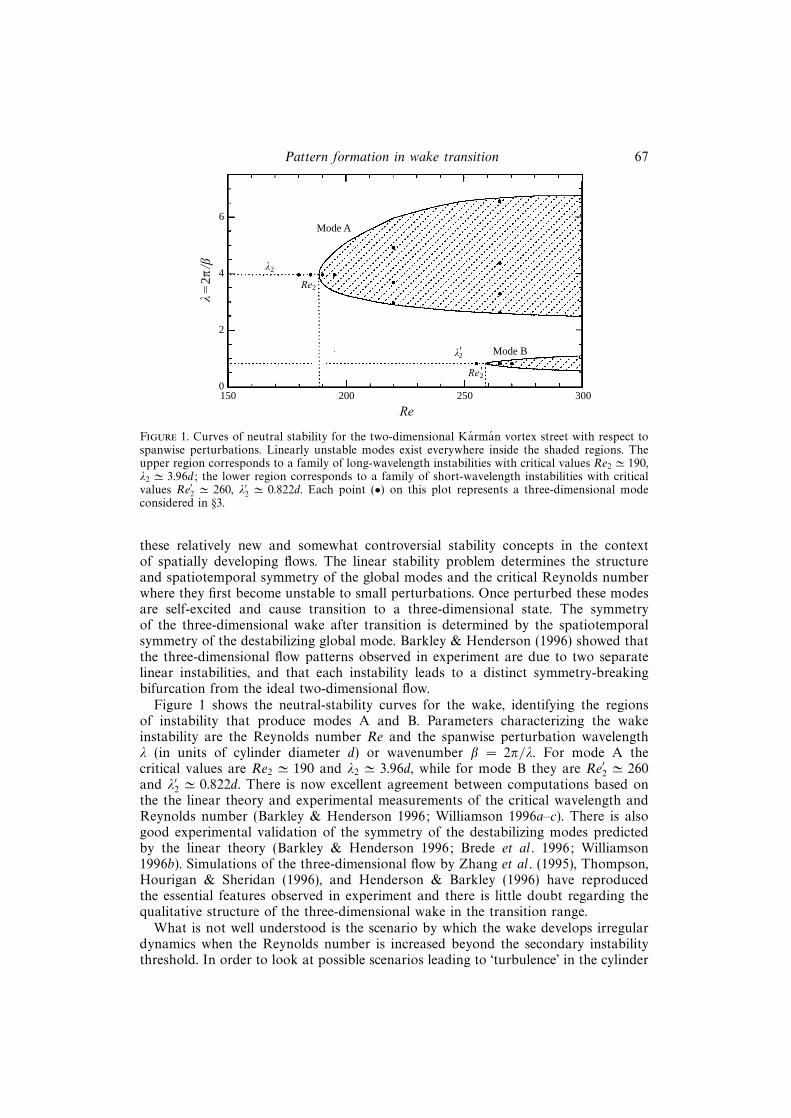
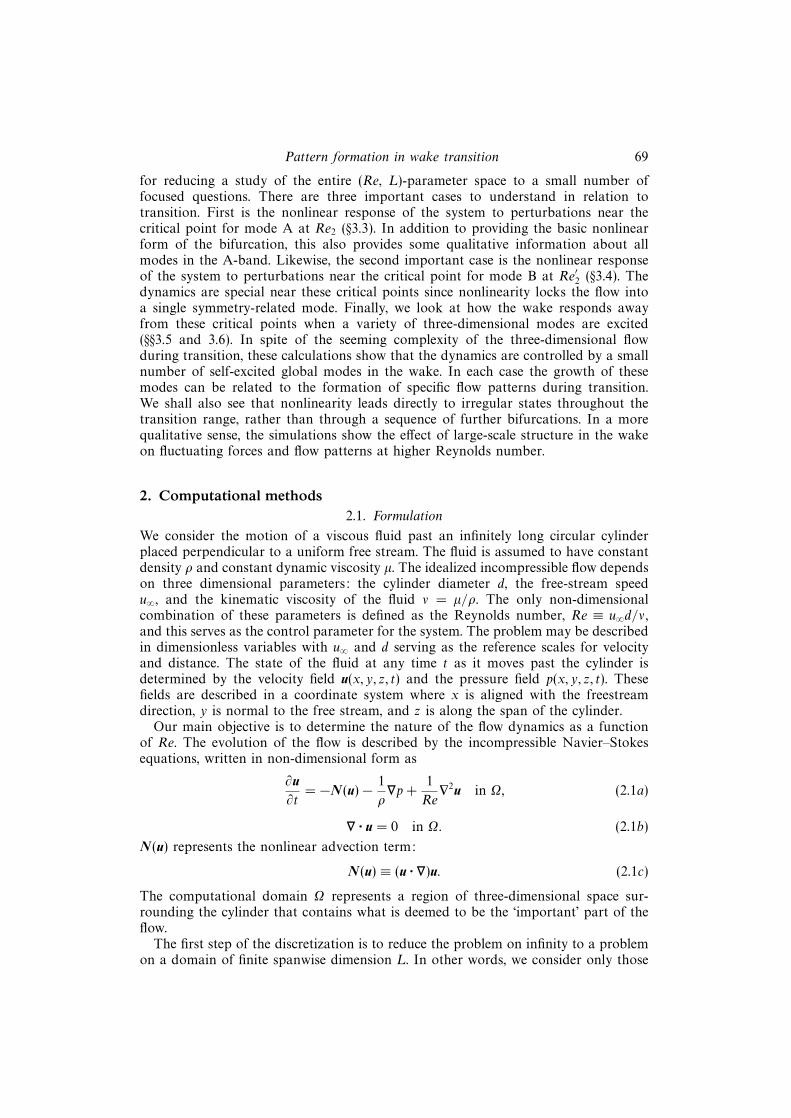

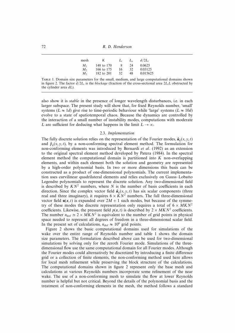
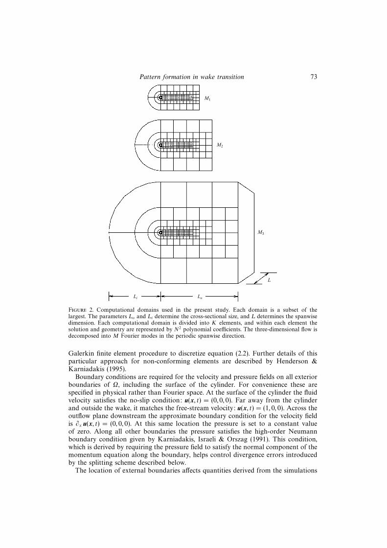
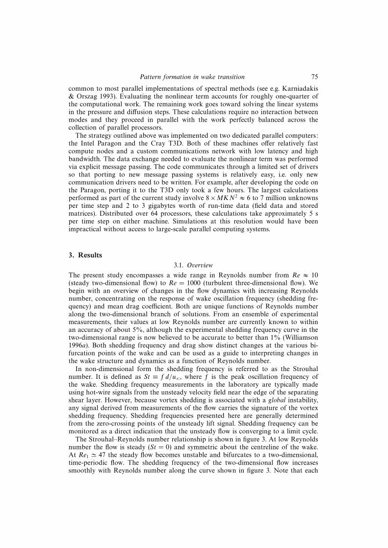
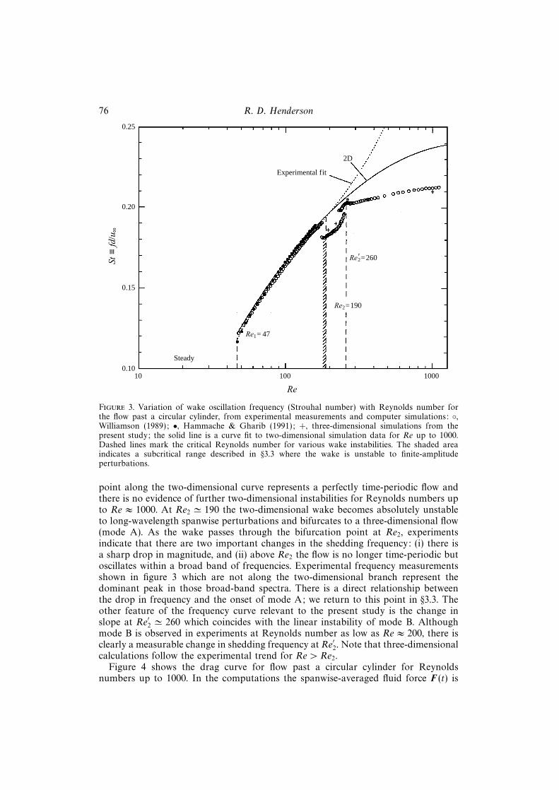
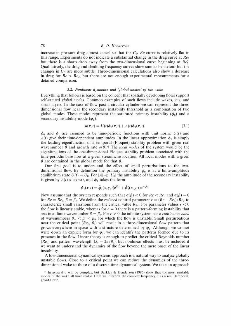
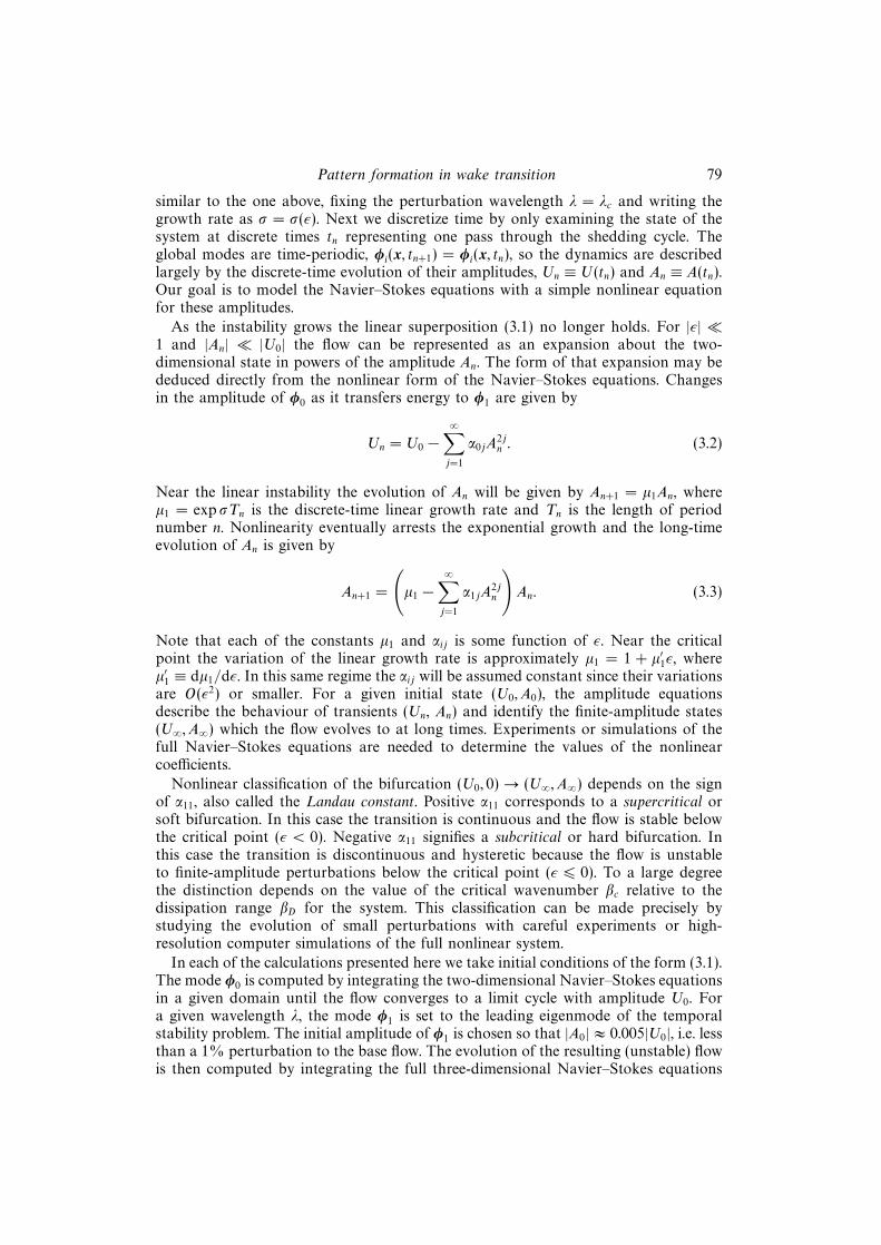

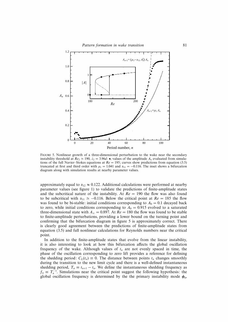

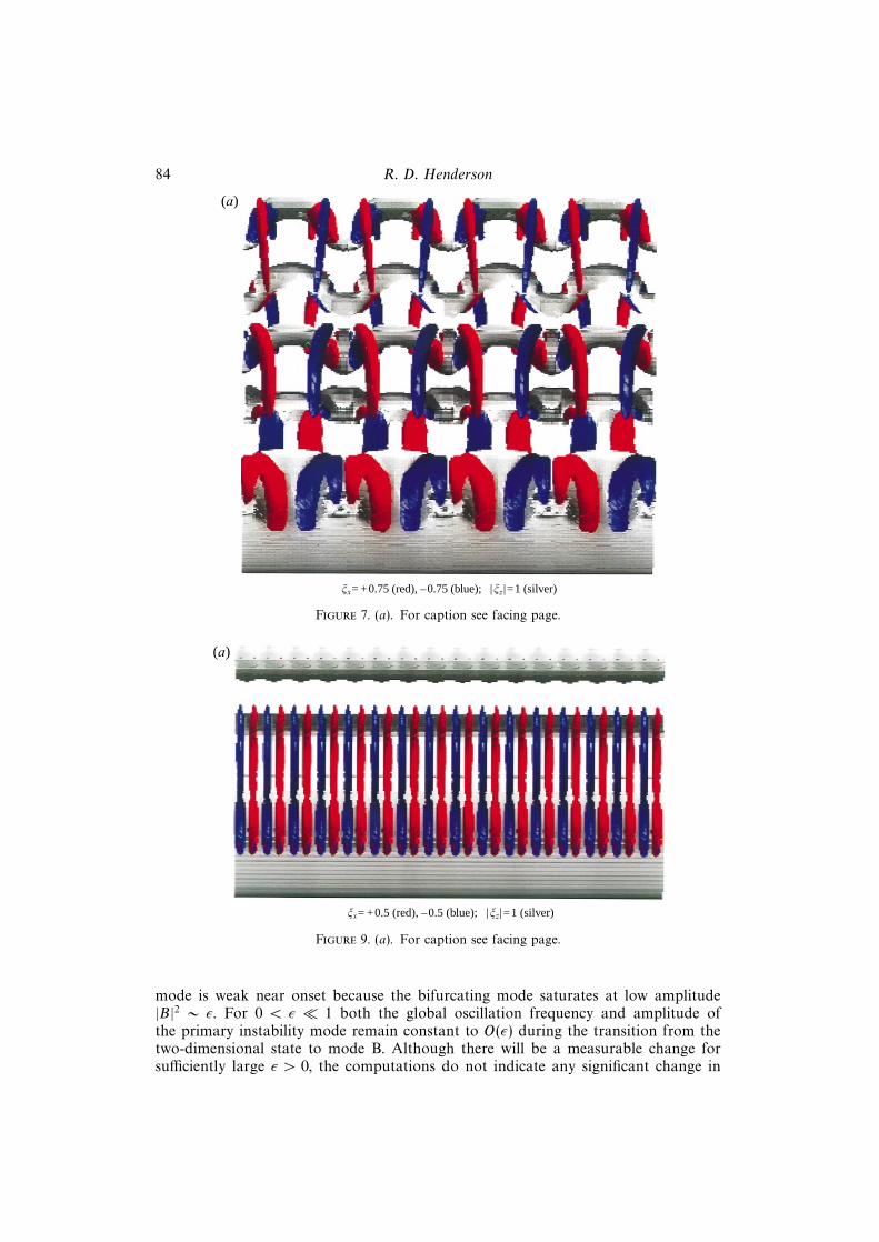
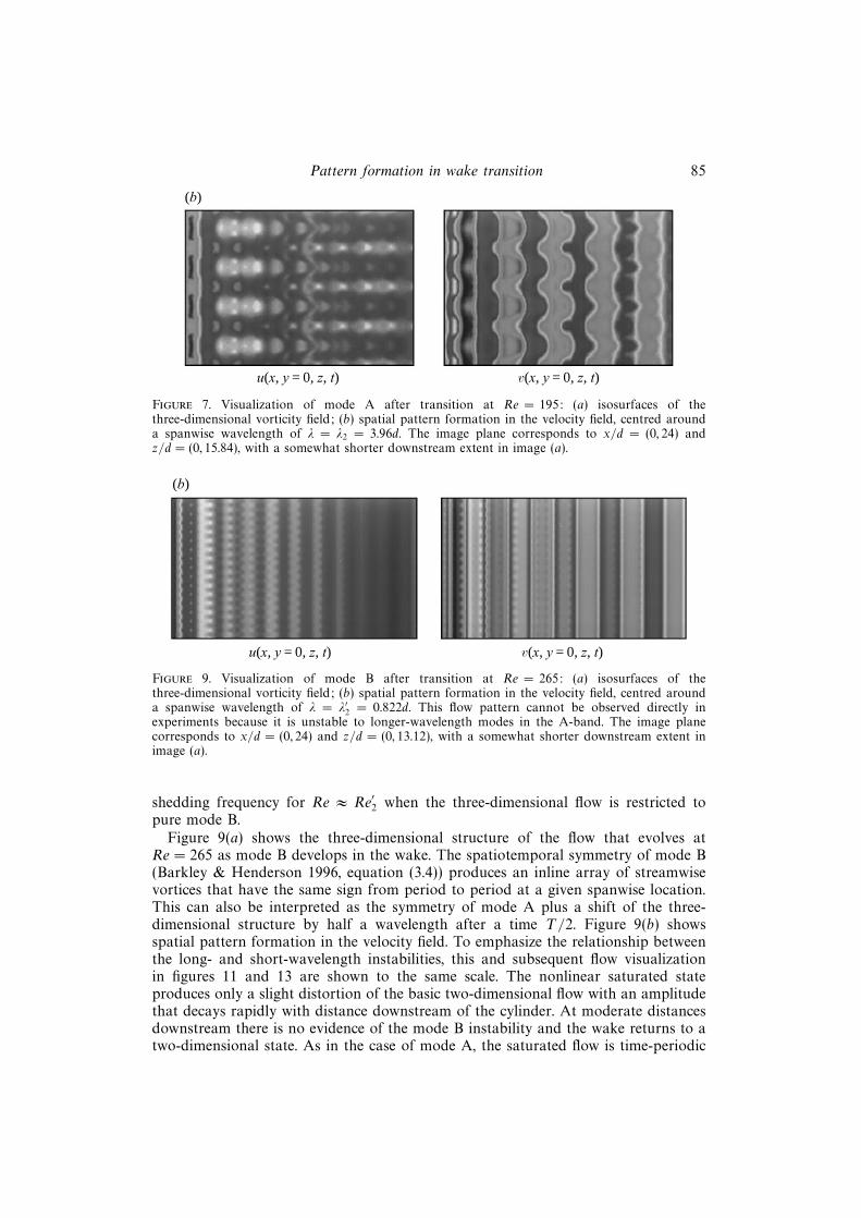
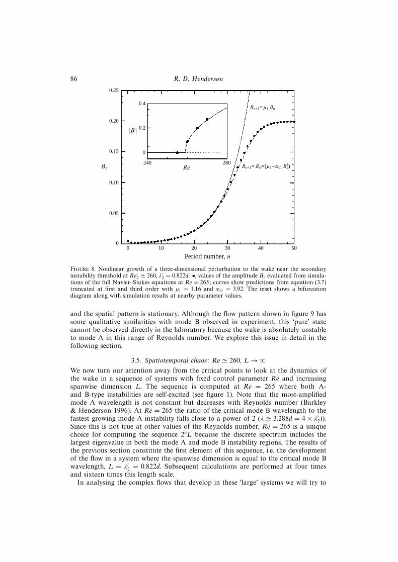
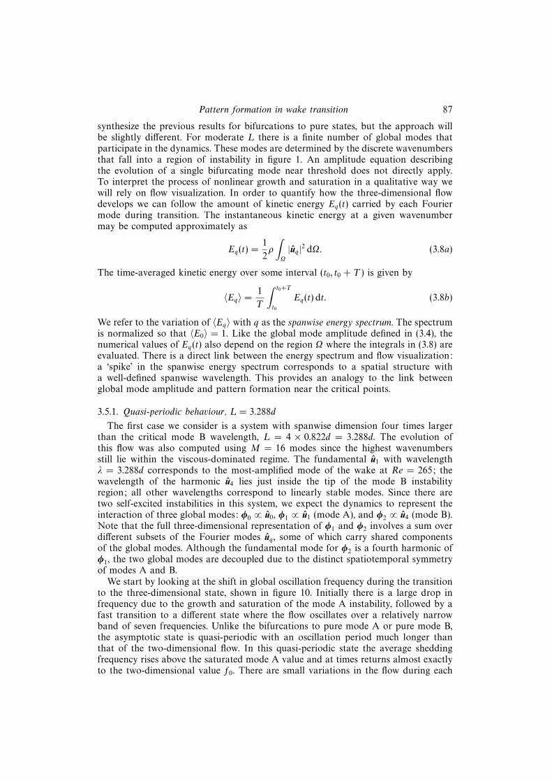

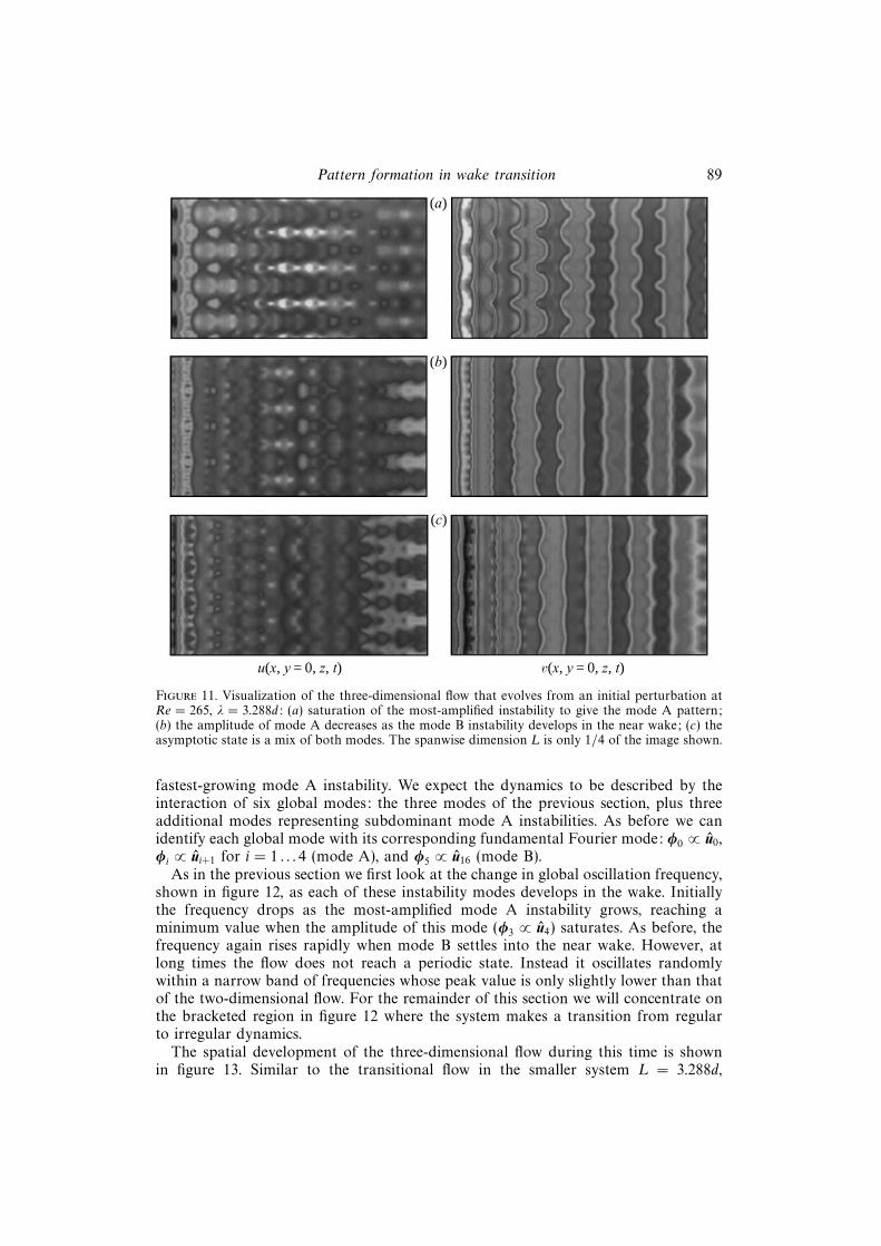
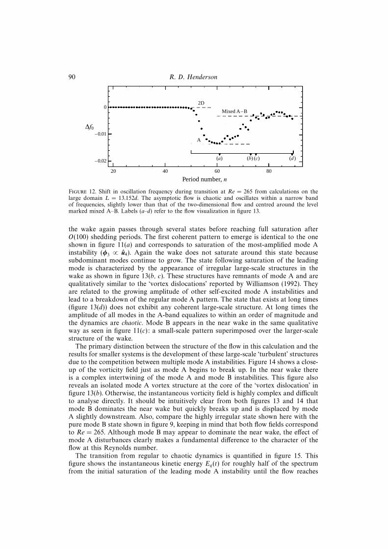
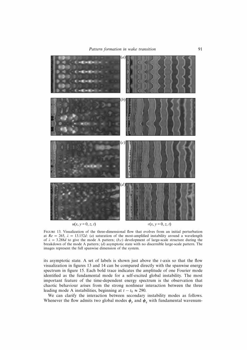
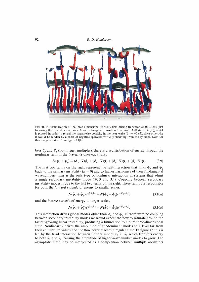
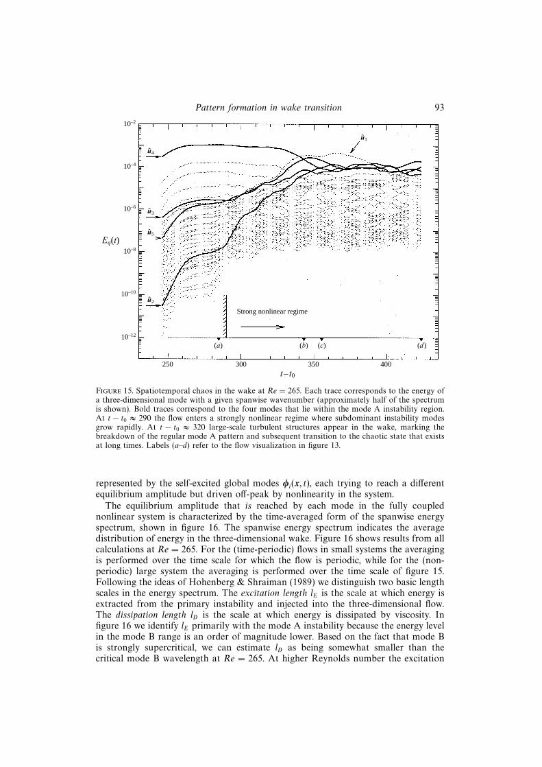
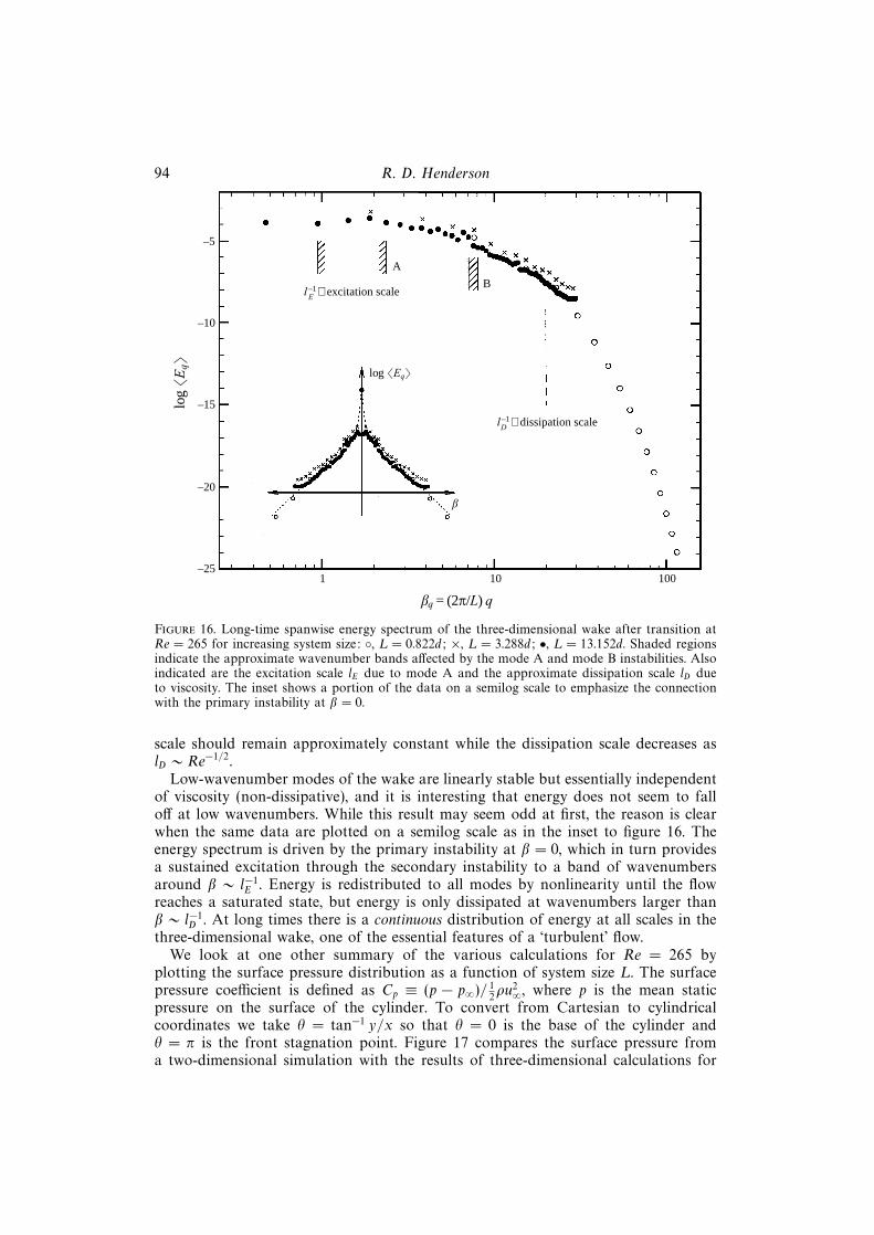
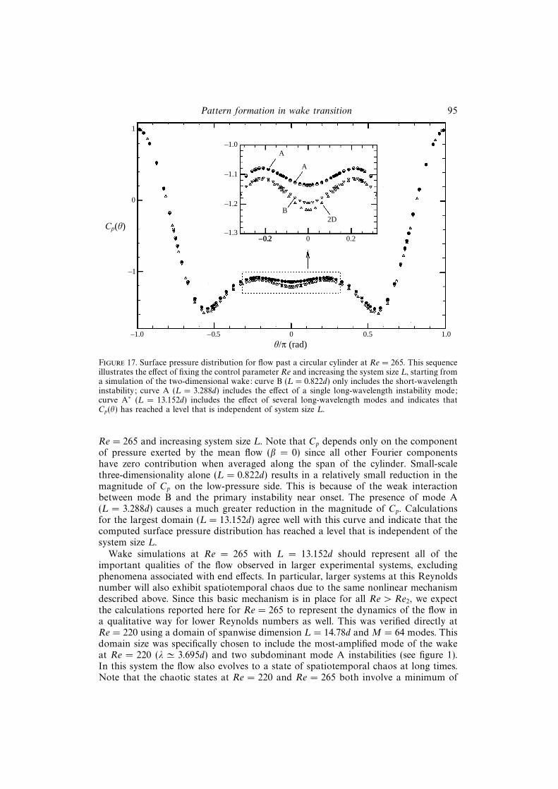
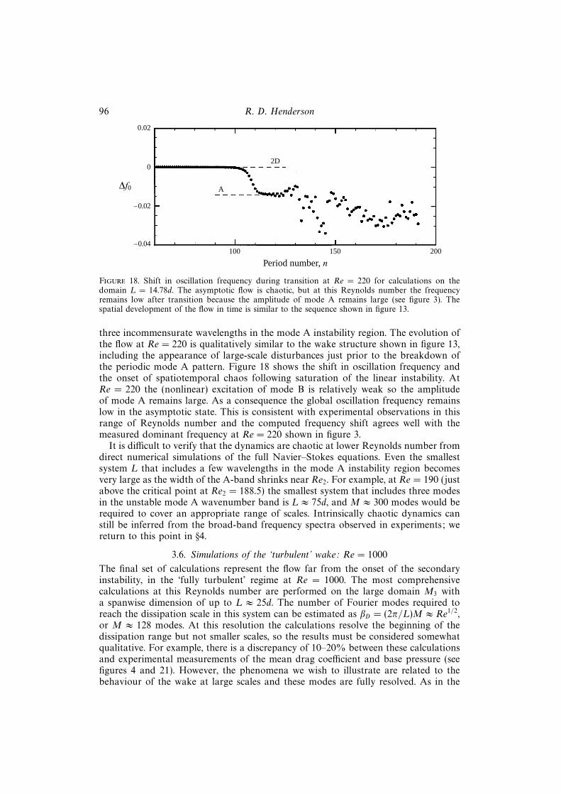
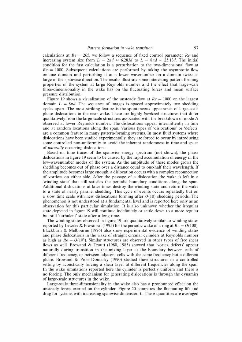
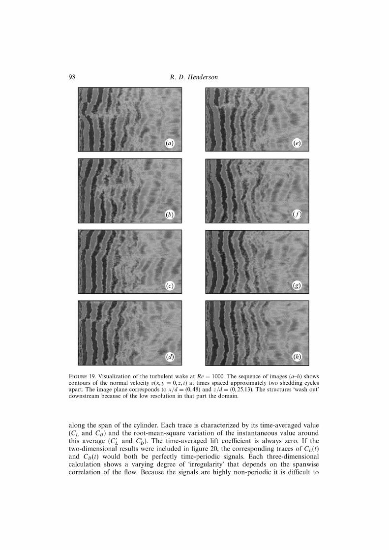
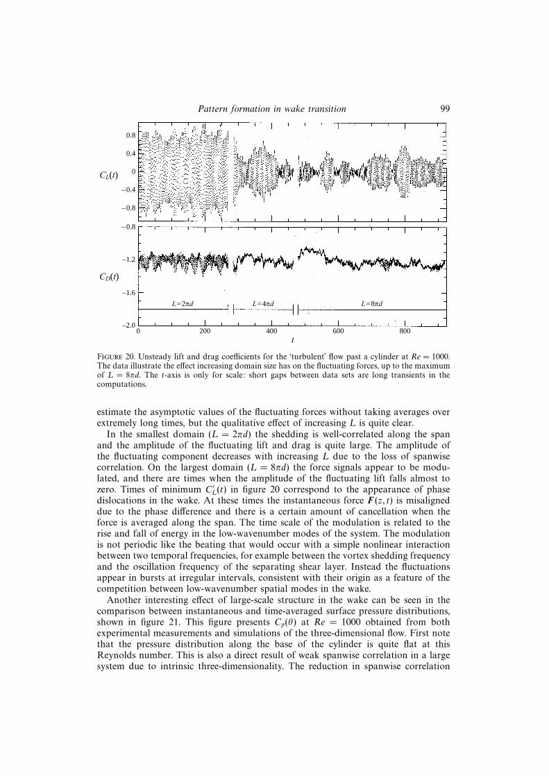
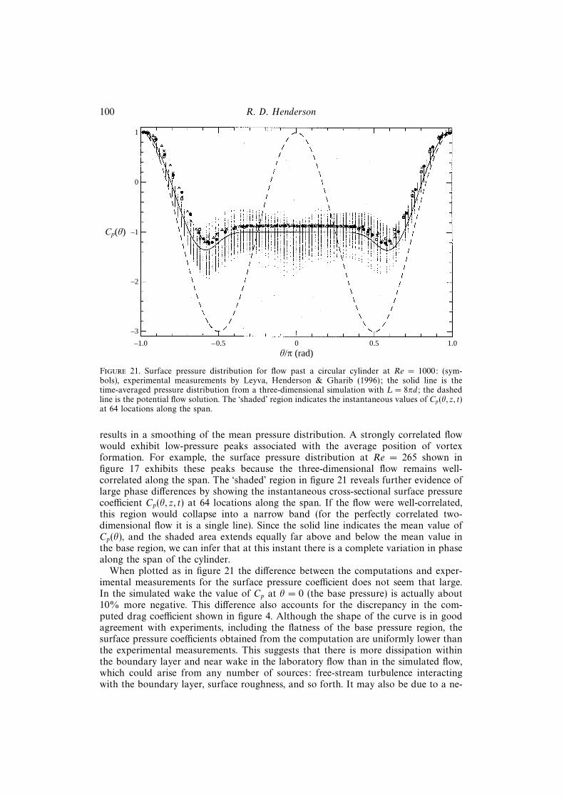
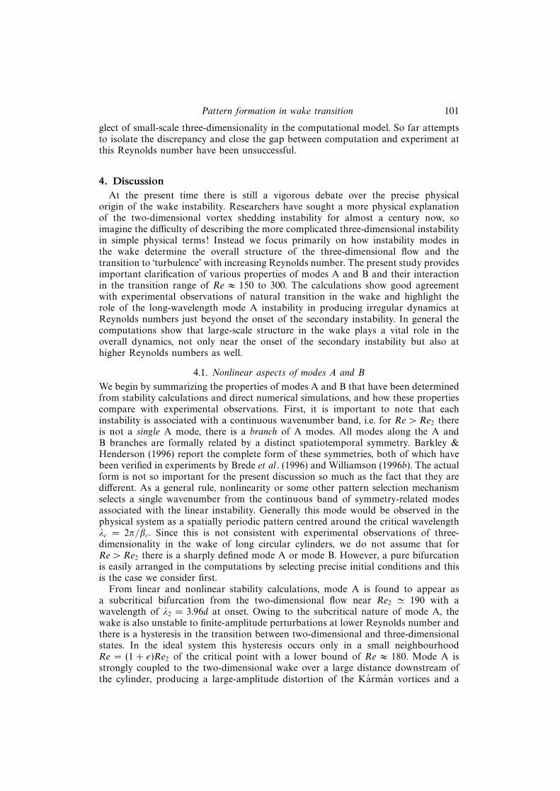
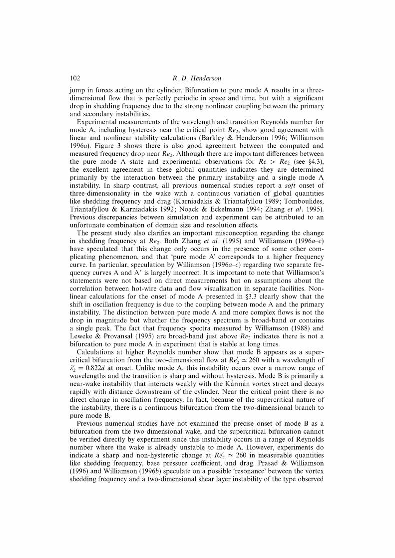
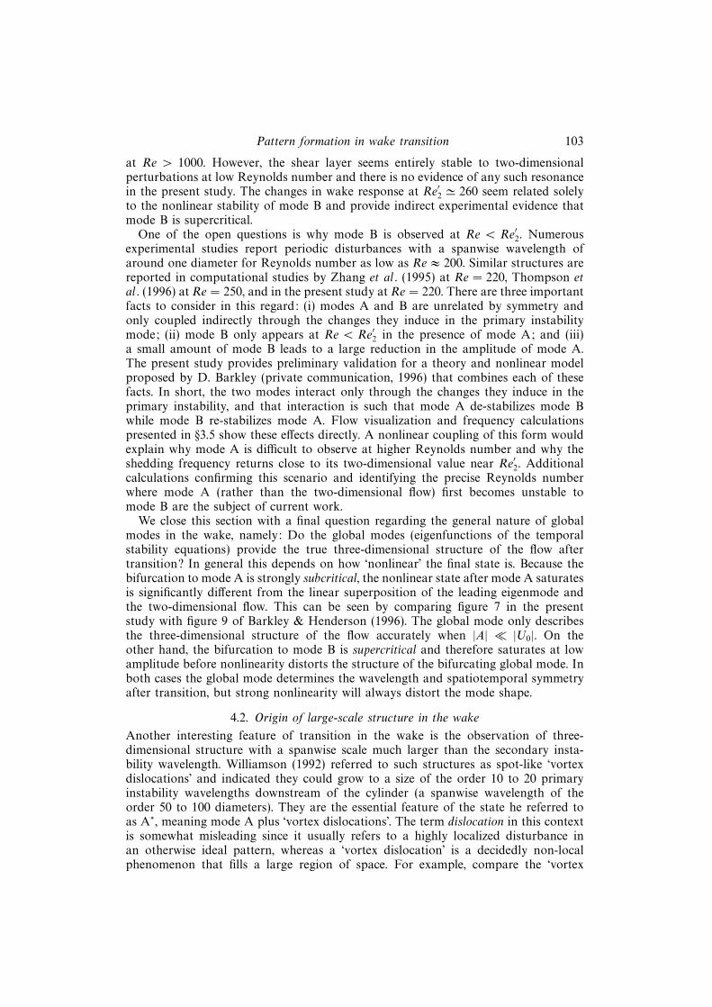
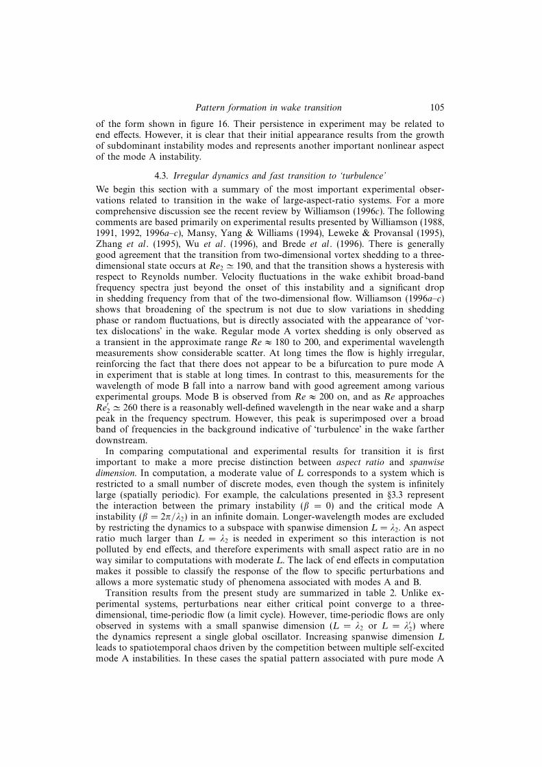
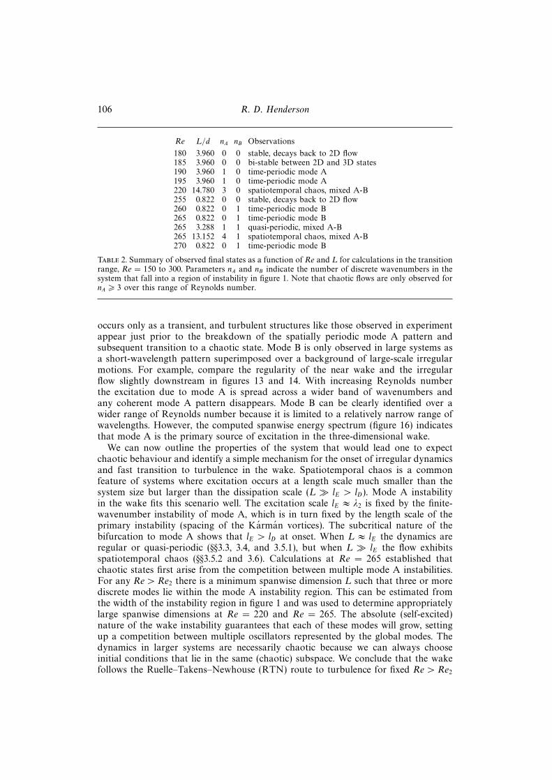
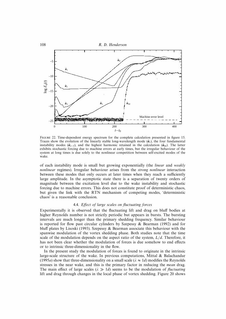


![Multidimensional Plasma Wake Excitation in the Non-linear ...1607.03514.pdf · become turbulent in multidimensions [8]. The electromagnetic structure of the plasma wakefield depends](https://static.documents.pub/doc/80x56/600f31fba4dc6e4cc30c1f16/multidimensional-plasma-wake-excitation-in-the-non-linear-160703514pdf-become.jpg)


