1

Nonlinear Finite Element Model Updating of an Infilled Frame Based on

Identified Time-varying Modal Parameters during an Earthquake

Eliyar Asgarieha, Babak Moavenib, and Andreas Stavridisc

a Ph.D. Candidate, Dept. of Civil and Environmental Engineering, Tufts University, Medford, Massachusetts, USA; E-mail: eliyar.asgarieh@tufts.edu

b Corresponding Author. Assistant Professor, Dept. of Civil and Environmental Engineering, Tufts University, Medford, Massachusetts, USA; E-mail: babak.moaveni@tufts.edu

c Assistant Professor, Dept. of Civil Engineering, University of Texas at Arlington, Arlington, Texas, USA; E-mail: stavridis@uta.edu

ABSTRACT

A model updating methodology is proposed for calibration of nonlinear finite element (FE)

models simulating the behavior of real-world complex civil structures subjected to seismic

excitations. In the proposed methodology, parameters of hysteretic material models assigned to

elements (or substructures) of a nonlinear FE model are updated by minimizing an objective

function. The objective function used in this study is the misfit between the experimentally

identified time-varying modal parameters of the structure and those of the FE model at selected

time instances along the response time history. The time-varying modal parameters are estimated

using the deterministic-stochastic subspace identification method which is an input-output

system identification approach. The performance of the proposed updating method is evaluated

through numerical and experimental applications on a large-scale three-story reinforced concrete

frame with masonry infills. The test structure was subjected to seismic base excitations of

increasing amplitude at a large outdoor shake-table. A nonlinear FE model of the test structure

has been calibrated to match the time-varying modal parameters of the test structure identified

2

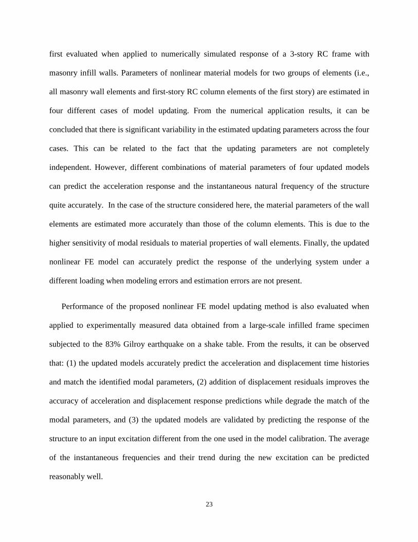
from measured data during a seismic base excitation. The accuracy of the proposed nonlinear FE

model updating procedure is quantified in numerical and experimental applications using

different error metrics. The calibrated models predict the exact simulated response very

accurately in the numerical application, while the updated models match the measured response

reasonably well in the experimental application.

Keywords: Nonlinear FE model updating; time-varying modal parameters; Bouc-Wen hysteretic

material model; damage identification.

1. Introduction

In recent years, vibration-based structural identification methods have received increased

attention in the civil, mechanical, and aerospace engineering research communities with the

objective of developing methods that can identify structural damage at the earliest possible stage,

evaluate the performance of structures under future loading conditions, and estimate their

remaining useful life [1-3]. A common class of methods consists of finite element (FE) model

updating [4]. These methods update the parameters of a FE model of the structure by minimizing

an objective function that expresses the offset between FE-predicted and experimentally

measured response or features extracted from the response. Optimum solutions of the problem

are reached through sensitivity-based constrained optimization algorithms (local methods) or

methods capable of reaching the global minimum for the objective function. Linear FE model

updating methods have been used for damage identification of real-world, large-scale structures

with reasonable success [5-7]. Note that in these methods, structural damage is usually defined as

reduction of “effective” stiffness based on the linear response of structure before and after a

3

damaging event. In addition, the calibrated FE models are linear and therefore can only predict

the behavior of structures in their linear range of response.

While linear FE model updating has been successfully applied for predicting damage

indicated by loss of effective stiffness, nonlinear FE model updating can provide improved and

more accurate damage identification results (i.e., a more comprehensive measure of damage) and

can be additionally used as a tool for damage prognosis (to predict the remaining useful life of

structures). The need for implementing nonlinear FE model updating in preference to linear FE

model updating can be justified by the facts that: (1) all real-world structures are inherently

nonlinear, with high uncertainties in their nonlinear behavior, (2) the nonlinear response of a

structure to moderate-to-large amplitude excitations reveals more information about damage than

does the linear response to low amplitude excitations before and after damage, and (3) a well-

calibrated nonlinear FE model can be used for damage prognosis.

Kerschen et al. [8] provided a comprehensive literature review of nonlinear system

identification methods. The authors classified the nonlinear identification methods into the

following seven categories: time-domain methods, frequency-domain methods, time-frequency

methods, methods that by-pass nonlinearity using linearization, modal methods, black-box

methods, and structural model updating methods. Little work is available in the literature on

nonlinear FE model updating. Hemez and Doebling [9] discussed the need to validate numerical

models for nonlinear structural dynamics and some of the challenges involved in nonlinear

model updating. They introduced time-domain metrics for nonlinear model updating [10]. Song

et al. [11] proposed a method for updating the nonlinear FE model of a structural system based

on low amplitude ambient vibration data. Schmidt [12] performed nonlinear FE model updating

of systems with local nonlinearities, such as Coulomb friction, gaps, and local plasticity, by

4

matching simulated and measured response time histories using modal state observers. Kapania

and Park [13] proposed the “time finite element method” for parametric identification of

nonlinear structural dynamic systems. Meyer et al. [14] performed identification of local

nonlinear stiffness and damping parameters based on linearized equations of motion using the

harmonic balance method to achieve a suitable model description in the frequency domain.

In application of nonlinear model updating for civil structures, nonlinearity can be defined by

the hysteretic material behavior at the element level. Therefore, the problem of identifying a

time-variant system is transformed to the problem of identifying time-invariant parameters of

hysteretic material models, which has been shown to be appropriate for representing real-world

civil structures. Kunnath et al. [15] have used time-domain methods to identify hysteretic

material behavior of civil structures as parameters of hysteretic models. In [16-22], parameters of

nonlinear material behavior have been identified in non-physics based models such as state-space

representation of structures by means of different adaptive time-domain methods such as

adaptive least squares and Kalman filter (KF). Since response data usually includes a

considerable amount of nonlinearity in these applications, revised versions of Kalman filters

such as the extended Kalman filter [18, 19] and the unscented Kalman filter [20, 21] are applied.

The extended Kalman filter is based on linearizing the model to the first order of accuracy, while

the unscented Kalman filter and particle filters [22] contain higher orders of accuracy for

nonlinear problems. However, most of these applications have been on single-degree-of-freedom

or simple multi-degree-of-freedom numerical examples. Therefore, there is a need for applying

nonlinear model updating methods to complex systems such as large-scale real-world civil

structures.

5

This paper proposes a practical method for nonlinear FE model updating of complex real-

world structures based on low dimensional features extracted from nonlinear response, i.e., time-

varying modal parameters at a number of points along the response time history. Time-varying

modal parameters are estimated using the deterministic stochastic subspace identification (DSI)

method [23] over short windows (0.5 second) of data around the considered time instants. The

nonlinearity is defined in the model by assigning Bouc-Wen hysteretic material behavior to

certain elements or groups of elements. Elements of similar material and cross-sections are

considered to have similar nonlinear behavior and are grouped together to reduce the number of

updating parameters. Selected parameters of Bouc-Wen models for each group of elements are

updated to minimize an objective function based on the difference between the time-varying

modal parameters of the FE model and the identified values at selected points along the response

time history. Finally, the performance of the proposed method is evaluated when applied to

numerical as well as experimental case studies. The considered case study is a 2/3-scale, 3-story

reinforced concrete frame with masonry infills which was subjected to several scaled ground

motions on a shake table. The accuracy of the proposed method in predicting the response and

the instantaneous modal parameters is quantified in the numerical application and the challenges

for applying this method to a large-scale complex structure are discussed when it is applied to the

experimental data.

2. Test Structure Specimen and Numerical Model

2.1. Test structure and Dynamic Tests

The structure considered here is a 2/3-scale, 2-bay, 3-story reinforced concrete moment-

frame with unreinforced masonry infill walls. The specimen, shown in Figure 1, was tested on

6

the large outdoor shake table at the University of California San Diego (UCSD). The structure

included slabs that simulated the scaled gravity mass of the external frame of the prototype while

accounting for the 2/3 length scale factor. To account for the effect of the seismic mass not

included in the specimen, the input ground acceleration time histories had to be scaled in time

and amplitude to satisfy the similitude requirement for the seismic forces. The design details and

resulting scale factors for the basic quantities are summarized in [24]. It should be noted that the

ground motion levels referred to in this paper correspond to the full-scale prototype structure.

The structure was damaged progressively by scaled records of the 1989 Loma Prieta earthquake,

measured at Gilroy 3 station (referred to Gilroy record in this paper). For the current study, the

structure’s response to seismic base excitation tests with 67% and 83% of Gilroy earthquake are

considered. The structure was densely instrumented with a large array of sensors, including

strain gages, string potentiometers, linear variable differential transformers (LVDTs), and

uniaxial accelerometers. However, only three acceleration measurements at each floor level (two

vertical and one longitudinal) are used in this study. More details about the structure, its

instrumentation and the shake table tests are available at [24, 25]. Figure 2 shows the horizontal

roof acceleration response history of the specimen during the considered earthquakes while the

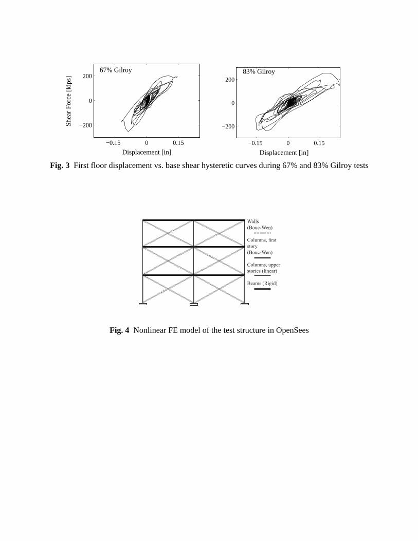
corresponding first floor displacement versus base shear hysteresis curves are plotted in Figure 3.

2.2. Numerical FE Model

A two-dimensional nonlinear FE model of the test structure, as shown in Figure 4, is created

in the structural analysis software OpenSees [26]. In this model, the beams are assumed as

linear-elastic Euler-Bernoulli frame elements, with their stiffnesses increased to act as rigid

elements. The increased stiffness accounts for the in-plane rigidity of the infills that do not allow

deformation of the beams. The infilled walls are modeled as struts using truss elements with

7

nonlinear material behavior. The columns of the first story are assumed to have nonlinear

material behavior, while the columns of the second and third stories are modeled as linear-elastic

frame elements since their deformations were found to be small even during large amplitude

seismic base excitations. Fiber elements with distributed plasticity are used for all nonlinear

elements with Bouc-Wen (-Baber-Noori) [27-30] hysteretic behavior assigned at the fiber

sections. For the purpose of nonlinear model updating, the elements are divided into two groups

based on their materials, namely the masonry infill walls and the reinforced concrete (RC)

columns of the first story. However, for calibration of the initial stiffness through a linear model

updating, the linear-elastic columns of the second and third stories are considered as the third

group of elements in the updating process.

The Bouc-Wen model is a class of phenomenological models that are widely used to

represent the hysteretic behavior (as lumped or distributed plasticity) of structural components

made of different materials. Several extensions of the Bouc-Wen models have been proposed in

the literature [28-32]. Their calibration typically requires from 5 up to 13 parameters depending

on whether stiffness degradation, strength degradation or pinching behavior are considered in the

model. The shapes and characteristics of the Bouc-Wen hysteresis curves are defined by these

time-invariant parameters in its formulation. To briefly review the applied Bouc-Wen model,

consider the second order differential equation of motion of a nonlinear dynamic system with

hysteretic material nonlinearity:

( ) ( ) ( , ) ( )t t t t+ + =Mx Cx R x u (1)

where u(t) is the vector of forcing functions, x(t) is the displacement response, M and C are the

mass and the viscous damping matrices, and R(x, t) corresponds to the nonlinear restoring force

8

vector at time t. The nonlinear restoring force at each single-degree-of-freedom (axial) fiber

using Bouc-Wen (-Baber-Noori) model is represented as:

( )0 0( , 1)R x t K x K zα α= + − (2)

where K0 is the initial tangent stiffness, α is the post yield to initial stiffness ratio, and z is the

virtual hysteretic displacement which can be obtained from the following first order differential

equation:

[1 ( )( ) ]( )

nx zhz x t zt xz

ν β γη

= − +

(3)

In Equation (3), β and γ affect the level of nonlinearity and shape of the hysteretic model; h

defines the pinching effect; η and ν control the stiffness and strength degradations, respectively,

and are defined based on the hysteretic energy ε.

( ) 1.0 ( )( ) 1.0 ( )t tt t

ν

η

ν δ εη δ ε

= += + with

0

( )t

t zxdtε = ∫ (4)

One of the main shortcomings of the Bouc-Wen models is the fact that the model parameters

are not independent. Due to the redundancy of parameters in this model, similar model responses

can be generated by different combinations of the model parameters. This dependency causes

difficulties in solving the inverse problem [31]. The sensitivities of output responses to different

Bouc-Wen model parameters have been investigated by several researchers [32, 33]. Based on

these studies and according to the authors’ past experience, only α, β, γ, and ηδ parameters are

chosen for updating in each group of nonlinear elements (wall and columns). No pinching effect

and strength degradation is considered in this study, i.e., h = 1 and 0vδ = .

9

3. System identification

The time-varying modal parameters of the test structure are identified at selected time

instances of the response time history. The system identification is performed using the

windowed DSI method [23] based on 0.5-second long windows of the measured data around the

considered time instances. The DSI method is a parametric system identification method that

“realizes” a stochastic state-space representation of a linear dynamic system using the input-

output data. The method is robust against the input disturbance and measurement noise since

both terms are explicitly included in its formulation. The identified modal parameters at each

time instance correspond to those of an equivalent linear system that represent the nonlinear

structure linearized at that time window, i.e., the identified system corresponds to a linear system

with effective stiffness of the structure over the considered 0.5 second time interval. The

performance and accuracy of the windowed DSI for instantaneous/short-time modal

identification was studied in a previous work by the authors [34].

Figure 5 shows the identified time-varying natural frequencies of the considered test structure

for the first two longitudinal modes at 17 points along the 83% Gilroy earthquake base

excitation. These 17 time instants are selected subjectively with emphasis on the larger amplitude

part of the response with moderate to high nonlinearity. From Figures 5, it can be observed that

the identified natural frequencies of the specimen drop significantly during the strong motion

part of the base excitation (12-15 seconds), but slowly increase as the vibration weakens. This

increase in the natural frequencies corresponds to an increase in the effective stiffness of the

structure at lower response amplitudes. However, there is a small reduction in the natural

frequency of the structure from before to after the earthquake due to permanent damage. Figure 6

shows the mode shapes of the first two longitudinal modes identified at t = 13.25 second of the

10

83% Gilroy earthquake, which is one of the selected points at the strong motion part of the

excitation. The identified natural frequencies and mode shapes of the two longitudinal modes at

these 17 instances are used for the nonlinear FE model updating of this test structure. It should be

noted that the identified windowed natural frequencies depend on the considered window length

and selected time instances. However, the corresponding natural frequencies of the FE models

are also computed using the same window length and at the same times.

4. Nonlinear FE Model Updating

Parameters of the nonlinear FE model are updated in order to minimize the difference

between the time-varying modal parameters from the model and those identified from the data.

An objective function ( )G θ is defined as a weighted sum of the modal parameter residuals at the

selected time instances along the nonlinear response.

2

1 1 1 1( ) ( ) ( ) ( ) ( )

t t t rN N N NT

t t t t tj tjt t t j

G g w r= = = =

= = =∑ ∑ ∑∑θ θ r θ Wr θ θ

(5)

In Equation (5), θ represents the vector of updating parameters (Bouc-Wen model parameters

for different groups of elements), ( )tr θ denotes the modal residual vector at time t, Wt is a

diagonal weighting matrix, Nt corresponds to the number of time instances, and Nr is the number

of considered residuals at each time instance and depends on the number of vibration modes and

sensor measurements. The residual vector ( )tr θ in the objective function contains the

eigenfrequency residual ( )ftr θ , and mode shape residual ( )s

tr θ , which are defined as

( , ) ( ) ( , ) ( )( )( ) , ( ) , ( ) ( ), {1 2 }

( , ) ( )( )( )

− Φ Φ = = = − ≠ ∈ Φ Φ

θ θr θr θ r θ r θ

θr θ

l lfj j j jf st

t t t mr rsj jjt

t t t tl r j N

t ttλ λ

λ (6)

11

where ( , )θj tλ and ( )

j tλ denote the FE-predicted and experimentally identified eigenfrequencies

for the jth vibration mode and at time t. Eigenfrequencies are defined as 2( ) 2 ( )j jt f tλ π , in

which ( )jf t is the corresponding natural frequency at time t, ( , )Φ θj t and ( )Φ j t denote the FE

predicted and experimentally identified mode shape vectors at time t. For each vibration mode,

the mode shapes ( , )Φ θj t and ( )Φ j t are normalized with respect to the same reference

component. The superscript r indicates the reference component of a mode shape vector and the

superscript l refers to the mode shape components that are used in the FE model updating

process, which in this case correspond to the degrees of freedom with sensor measurements. Nm

is the number of vibration modes considered in the updating process. In this study, the first two

longitudinal modes are used in the objective function (i.e., Nm = 2).

The FE model updating is performed in two steps:

(1) In the first step, the initial tangent stiffnesses of elements ( 0K in Equation 2) in three

substructures/groups of elements (walls, columns of the first story, and columns of the second

and third stories) are updated using the identified modal parameters at one point during the low-

amplitude part of response at the beginning of the excitation. Due to small amplitude of the

response during this time window, the structure is assumed to behave linearly and therefore the

identified modal parameters correspond to the initial tangent stiffness. This first step is a linear

FE model updating and the optimal values of updating parameters are achieved by using the

simulated annealing global optimization method, which is a probabilistic method based on

Monte Carlo simulations [35].

(2) In the second step, parameters of the nonlinear material model for the two considered

substructures (walls, columns of the first story) are estimated using the identified modal

12

parameters at the 17 selected points along the response time history. In the experimental

application, the first two of these 17 points are selected at the beginning of the record with low

level of response nonlinearity, the next four points (3-6) are during the strongest part of

excitation with the highest level of nonlinearity, points 7-11 are during the moderate amplitude

excitation with low to moderate levels of nonlinearity in response, and the last six points (12-17)

are at the end of excitation with low level of nonlinearity (see Figure 5). The simulated annealing

global optimization algorithm is used to find the model parameters that minimize the objective

function.

5. Model Updating Results

5.1. Application to Numerically Simulated Data

In this section, performance of the proposed nonlinear FE model updating is evaluated when

applied to numerically simulated data assuming no measurement noise and modeling errors. The

data used in this section is generated using a nonlinear FE model of the structure described in

Section 2.2. The FE model, from this point on referred to as the baseline model, has been created

in OpenSees and its role is to provide data for the evaluation of the model updating algorithm.

Note that this is not an accurate model of the specimen, but rather a sufficiently good model that

is used as an intermediate step prior to applying the proposed algorithm to the data from the

physical specimen which is discussed in the following section. The numerical model of the

structure is subjected to the 100% Gilroy earthquake record measured on the shake table which

has been scaled in time and amplitude according the scaling factors discussed earlier [24].

Figure 7 shows the roof acceleration and the time history of instantaneous natural frequencies

for the first two modes obtained when the model is subjected to this record. The numerical data

13

is recorded at the same locations that the corresponding sensors were installed in the physical

specimen for consistency. Time-varying modal parameters of the structure are estimated at 17

arbitrarily selected points along the response time history. These points are different from the 17

points used in the experimental application that is based on the 83% Gilroy record shown in

Figure 5. For the case of the experimentally measured data, the points fall within a shorter length

of measured signals in comparison to the numerically generated data because of the smaller

signal-to-noise ratio of measurements at the beginning and at the end of the excitation, during

which the modal parameters of the structure are not observable. Figure 8 plots the “identified”

natural frequencies of the first two modes at these 17 points. In the numerical application, the

average of exact instantaneous modal parameters over 0.5-second time windows are used as the

“identified” values so that the method is consistent with that used for the experimental data. The

identified natural frequencies and mode shapes of the structure are used to form the residuals in

the objective function (see Equations 5 and 6).

The first step of model updating, as described in the previous section, is to estimate the initial

tangent stiffness for the three considered groups of elements, namely (1) the strut elements

representing the masonry walls, (2) the columns of the first story, and (3) the columns of the

second and third stories. The identified modal parameters at time t = 5.0 seconds, at which the

model practically behaves linearly, are used for estimating the values of initial stiffness. Table 1

reports the stiffness (Young’s moduli) for the three updating groups of elements for the updated

and the baseline model. It can be observed that the stiffness parameters of the walls and the first

story columns are estimated accurately while larger estimation error is obtained for stiffness of

the upper story columns. This implies lower sensitivity of the considered residuals to the

stiffness of this group of elements. Figure 9 compares the roof acceleration response of the

14

updated model with its exact counterpart during the low amplitude part of the response at the

beginning of the earthquake when the response is practically linear. The reproduced response

using the updated FE model is in excellent agreement with the response of the baseline model

indicating the accuracy of the updated model during low amplitude response.

In the second step of the proposed model updating method, parameters of the nonlinear

material models for two groups of elements; the first-story masonry wall elements and the first

story columns are estimated. The upper story walls and columns are not considered here as they

are deemed to behave linearly. Considering the flexibility of the Bouc-Wen model, four distinct

updating cases have been considered at this step:

Case (1): Three parameters α, β (= γ), and ηδ are updated for each substructure resulting in a

total of six updating parameters using the modal parameter residuals at 17 selected points.

Case (2): Four parameters α, β, γ, and ηδ are updated for each substructure resulting in a total of

eight updating parameters using the modal parameter residuals at 17 selected points.

Case (3): Three parameters α, β (= γ), and ηδ are updated for each substructure resulting in a

total of six updating parameters; however updating is performed in an iterative manner. In the

first iteration, α and β (= γ) controlling the post-yield stiffness and the shape of the hysteretic

model, respectively, are estimated based on the points in the high or moderate amplitude part of

the response (all points except the two initial points and two final points, which means 13 points

in the middle). In the second iteration, stiffness degradation parameters ηδ are estimated (while

other parameters are fixed) based on the modal parameters at the two initial and two final time

instances. These iterations are repeated consecutively until no significant reduction in the

objective function is observed.

15

Case (4): Similar to Case 3 but in the first iteration, three parameters α, β, and γ are updated.

The estimated parameters from the updated model along with those of the baseline model are

presented in Table 2. From this table, it can be observed that (1) there is significant variability in

the estimated values of the material parameters across the four cases, and (2) in general,

parameters of the wall elements are estimated more accurately than those of the column

elements. This is due to the higher sensitivity of modal residuals to material properties of wall

elements. The accuracy of calibrated nonlinear FE models is quantified using five different error

metrics, namely the error in estimated model parameters (Eθ), the error in predicted

instantaneous natural frequency of the first mode (Ef), the error in predicted roof acceleration

response (Eacc), the error in predicted first story displacement response (Edis), and the value of the

objective function ( )G θ . Error in the estimated model parameters is defined as the normalized

sum of the difference between the updated parameters and those of the baseline model.

id baselinej j

baselinej j

Eθ

θ θ

θ

−= ∑ (7)

with idjθ and baseline

jθ referring to the identified and baseline Bouc-Wen parameters. The error

metrics for the instantaneous natural frequencies, as well as displacement and acceleration

responses are defined as the normalized l2-norm of the discrepancies between model-predicted

response and the exact values. The response time histories between 10 and 35 second are

considered in computation of these norms:

model measured

measuredE =x

x - x

x (8)

16

where xmodel and xmeasured correspond to the model predicted and baseline model vectors of

response time histories, and denotes the l2-norm. Table 3 reports these five error metrics for

the updated FE models in Cases 1-4. It is observed that (1) even though the estimated model

parameters do not necessarily match those of the baseline model, all four updated models predict

the acceleration response and the instantaneous natural frequency of the structure accurately, (2)

Case 1 provides the most accurate model in terms of all error metrics while the models from

Cases 3 or 4 can be the second best depending on which error metric is considered, and (3)

updating the degradation parameters iteratively in a separate step (Cases 3 and 4) does not

improve the results.

In Figure 10, the time histories of the instantaneous natural frequencies of the four calibrated

FE models over the most intense portion of the ground motion (12-14 seconds) are compared

with the values from the baseline model in the left column while the 0.5-second window

averaged natural frequencies of the models are compared with the identified values at the

considered 17 time instances in the right column. Overall, the instantaneous natural frequencies

of the updated models are in very good agreement with the exact values except for a few cycles

during the most nonlinear part of response for Cases 2-4. Figure 11 compares the roof

acceleration and first-story displacement responses of the four models with those of the baseline

model during the most demanding part of the excitation. In Figures 10 and 11 it can be observed

that the natural frequencies, as well as the response quantities, especially the roof acceleration, of

the updated models match well their counterparts obtained from the baseline model, even if the

model parameters are not identical. This can be related to the mentioned characteristics of the

Bouc-Wen models that the parameters of this material model are not completely independent

[31, 32]. Although in this study a small number of parameters are being updated, the model

17

updating methodology can yield different sets of material parameters that yield satisfactory

model behavior which is related to the choice of the constitutive law model. This is a very

important observation that one should keep in mind when calibrating numerical models. For

example, in the Bouc-Wen model there is a compensation effect between the degradation

parameter ηδ and β and γ that influence the shape of the hysteresis loops. Since the degradation

behavior in the Bouc-Wen model is defined based on the hysteretic energy (i.e., enclosed area by

the hysteresis loop) and ηδ , increasing β and γ (which results in larger hysteresis loops) will

have similar effects as decreasing ηδ . Dependency of the updating parameters as well as low

sensitivities of the residuals to these parameters can be the main sources of non-uniqueness

(unidentifiability) and estimation error of the model parameters. Figure 12 compares the base

shear force versus the first story displacement hysteretic plots for the four models. Case 1 model

provides an excellent match to the exact hysteretic behavior while other cases have some

prediction errors. This observation stresses the importance of a ‘good’ calibration of a numerical

model and provides insight as the criteria that should be used in the model updating algorithm

based on the use of the numerical model.

Finally, the updated FE models are validated by evaluating their performance in predicting

the response of structure to a base excitation different from the one used for model updating.

Figure 13 shows the predicted response using the updated model in Case 1 when subjected to

67% Gilroy base excitation. The predicted roof acceleration and first story displacement

responses, base shear force versus first story displacement hysteretic curve, and instantaneous

natural frequency of mode one are compared with their corresponding exact values. It is found

that the updated nonlinear FE model can accurately predict the response of the underlying system

18

under a different loading in this numerical application when modeling errors and estimation

errors are not present.

5.2. Application to Experimentally Measured Data

After the validation of the proposed nonlinear FE model updating method with numerically

generated data, its performance is evaluated with application to experimentally measured data of

the considered large-scale infilled frame specimen to the 83% Gilroy earthquake. The model

updating is performed in two steps as described in Section 4. In the first step, the initial stiffness

values of elements at three substructures are estimated using the identified modal parameters at

an instant at which the response is within the elastic range. Here the time t = 11 seconds has been

selected. The effective Young’s moduli for the walls, first-story columns, and higher story

column elements are updated as 3940, 2900, and 3690 ksi, respectively. Table 4 compares the

experimentally identified modal parameters of the first two modes with those from the updated

FE model after the first step. Modal parameters of the updated FE model are in excellent

agreement with the identified values, indicating the accuracy of the updated model in predicting

the low-amplitude response of the test structure at the beginning of the excitation.

In the second step, parameters of the two hysteretic material models are updated. The

identified windowed modal parameters including the natural frequencies and mode shapes of the

first two modes at 17 points along the response time history, as shown in Figure 5 and discussed

earlier, are used for updating the nonlinear material models in this step. From the four different

updating cases used in the previous section, Case 1 is considered for calibrating the nonlinear FE

model in this section as it was the most successful among the four cases. In this section, a new

Case 2 is defined by adding displacement residuals to the previously defined objective function

19

shown in Equation 5. The displacement residuals are calculated as the difference in model-

predicted and measured first story displacements at 10 selected points, which are mostly located

at the peaks of the response during its high amplitude part. The new objective function for Case 2

can be written as:

* 2

1( ) ( ) ( ( ))

( , ) ( )with ( )( )

=

= +

−=

∑θ θ θ

θr θ

dNd dt t

t

dt

G G w r

d t d td t

(9)

where *( )G θ is the new objective function, ( )dtr θ is the vector of displacement residuals at time

t, with total number of points Nd = 10, and displacement residual weights 1.dtw = ( , )θd t and

( )d t refer to the model-predicted and experimentally measured displacements at the first story.

In summary, Cases 1 and 2 in the experimental application of the proposed methodology are

defined as:

Case (1): Three parameters α, β (= γ), and ηδ are updated for each substructure resulting in a

total of six updating parameters using modal parameter residuals in the objective function ( )G θ .

Case (2): Three parameters α, β (= γ), and ηδ are updated for each substructure resulting in a

total of six updating parameters using modal parameter and displacement residuals in the

objective function *( )G θ .

Table 5 presents the estimated Bouc-Wen material parameters of the walls and first story

column elements for Cases 1 and 2 of nonlinear FE model updating based on experimental data.

It can be seen that the addition of the displacement residuals in the objective function affects the

values of estimated parameters. Table 6 reports the roof acceleration and first-story

20

displacement error metrics as well as the values of ( )G θ for the two updated models. The

acceleration and displacement error metrics in the experimental application are defined in a

manner similar as in the numerical application. The first-floor absolute horizontal displacement

was measured during the shake-table tests using LVDT sensors. From Table 6, it can be

observed that (1) the addition of displacement residuals improves the accuracy of acceleration

and displacement response predictions but it degrades the match between analytically predicted

and experimentally identified modal parameters, and (2) the error metrics in the experimental

application are significantly larger than those in the numerical application. This is mainly due to

fact that the performance of a complex structure is being simulated with a simplified FE model

(i.e., large modeling errors). The model used in this study is still more complex than those

typically used in engineering practice but involves a number of simplifying assumptions in

modeling the interaction between the infills and bounding frame that can be expected to result in

significant modeling errors; especially when the structure behaves highly nonlinear. Using more

detailed and complete FE models such as the one developed by Stavridis and Shing [36] can

reduce the modeling errors. However, more sophisticated models require a larger number of

updating parameters which makes the updating process more complicated and computationally

expensive. Another source of error in the experimental application of the proposed nonlinear FE

model updating method is the estimation uncertainty of the identified modal parameters from a

short-time window of data.

Figure 14 compares the model predicted roof acceleration and first floor displacement

responses with the measured values. Modal parameters of the updated models and the

experimentally identified modal parameters at the 17 time instances used for model updating are

shown in Figure 15. Figure 16 compares the model predicted and experimentally measured base

21

shear versus first floor displacement hysteretic curves. The predicted hysteretic curves here are

calculated by multiplying the total accelerations and masses of the floors, to be consistent with

their experimentally computed counterparts. From Figures 14 to 16, it can be observed that (1)

the updated models accurately predict the acceleration and displacement time histories and match

the identified modal parameters, (2) the addition of displacement residuals improves the

accuracy of predicted response time histories, and (3) the force-displacement hysteretic curves of

the models are in reasonably good agreement with those obtained from the experiment.

However, the error between model predicted and measured hysteretic curves is larger than the

error in response time histories or modal parameters.

Figure 17 shows the force-displacement hysteretic curves for the walls of each story and the

columns of the first-story predicted using the updated model in Case 1 due to the 83% Gilroy

record. It can be seen that the first story walls have the highest amount of nonlinearity, the

second story walls behave moderately nonlinear and the nonlinearity in the top story walls and

first story columns is low. The observation of the specimen [24, 25] indicated the appearance of

large cracks after the 83% Gilroy earthquake in the walls of the first story while negligible

damage was detected in the walls and columns of the second and third stories. Another

observation from inspection of test specimen is that some cracks have propagated from the walls

to the columns in the first story during the excitation. This observation is also verified by the

updated FE model as yielding at some sections of the columns is predicted in the model. The

material nonlinearity (e.g., due to crack propagation in concrete and masonry infills, and yielding

in steel rebars) is directly correlated with the amount of structural damage observed in the test

structure during the experiment [24, 25]. Therefore, a reasonably well-calibrated nonlinear FE

model can be used to predict the amount of nonlinearity (e.g., material yielding and stiffness

22

degradation) in a structure for a future excitation and this information in turn can be used for

damage diagnosis and reliability analysis.

Similarly to the numerical application, the updated models are validated by predicting the

response of the structure to an input excitation different from the one used for updating. Figure

18(a) and 18(b) show the predicted roof acceleration and first floor displacement response (using

the updated model in Case 1) to the 67% Gilroy record together with the measured time histories.

The updated model can predict the response of the structure to 67% Gilroy accurately for low to

moderate amplitude response while the prediction error increases for high amplitude part of

response. Figure 18(c) compares the base shear force versus first story displacement hysteretic

curves while the comparison between the identified and model predicted time-varying first mode

natural frequencies during this base excitation is shown in Figure 18(d). The average of the

instantaneous frequencies from the model can estimate the identified frequencies and their trend

reasonably well. The updated model seems to behave more nonlinearly than the actual specimen.

Therefore, the model-predicted peak displacement is larger than the measured peak

displacement.

6. Conclusions

A methodology for practical nonlinear FE model calibration of complex real-world civil

structures is proposed in this study. Parameters of material hysteretic models for different

substructures are updated to minimize an objective function that is based on the difference

between the time-varying modal parameters of the FE model and the identified values at selected

points along the response time history. The windowed DSI method is used to identify the time-

varying modal parameters at considered time instants. Performance of the proposed method is

23

first evaluated when applied to numerically simulated response of a 3-story RC frame with

masonry infill walls. Parameters of nonlinear material models for two groups of elements (i.e.,

all masonry wall elements and first-story RC column elements of the first story) are estimated in

four different cases of model updating. From the numerical application results, it can be

concluded that there is significant variability in the estimated updating parameters across the four

cases. This can be related to the fact that the updating parameters are not completely

independent. However, different combinations of material parameters of four updated models

can predict the acceleration response and the instantaneous natural frequency of the structure

quite accurately. In the case of the structure considered here, the material parameters of the wall

elements are estimated more accurately than those of the column elements. This is due to the

higher sensitivity of modal residuals to material properties of wall elements. Finally, the updated

nonlinear FE model can accurately predict the response of the underlying system under a

different loading when modeling errors and estimation errors are not present.

Performance of the proposed nonlinear FE model updating method is also evaluated when

applied to experimentally measured data obtained from a large-scale infilled frame specimen

subjected to the 83% Gilroy earthquake on a shake table. From the results, it can be observed

that: (1) the updated models accurately predict the acceleration and displacement time histories

and match the identified modal parameters, (2) addition of displacement residuals improves the

accuracy of acceleration and displacement response predictions while degrade the match of the

modal parameters, and (3) the updated models are validated by predicting the response of the

structure to an input excitation different from the one used in the model calibration. The average

of the instantaneous frequencies and their trend during the new excitation can be predicted

reasonably well.

24

Nonlinear FE model updating can provide improved and more accurate damage identification

results (i.e., a more comprehensive measure of damage) as compared to linear model updating.

The experienced amount of material nonlinearity (due to crack propagation in concrete, masonry

infills, and yielding in steel rebars) is a good measure of structural damage. Therefore, a

reasonably well calibrated nonlinear FE model can be used to predict the amount of nonlinearity

(e.g., material yielding and stiffness degradation) in a structure for a future excitation and this

information in turn can be used for damage diagnosis and reliability analysis.

ACKNOWLEDGEMENTS

The authors would like to thank Professor Benson Shing at UCSD for making the shake table

test data available for this study. Assistance of Dr. Ioannis Koutromanos as well as the technical

staff at the Englekirk Structural Engineering Center in collecting the test data used in this study

is also greatly acknowledged. The authors would also like to acknowledge Mr. Durwood

Marshall and his colleagues at Tufts UIT center for their assistance to set up the model updating

computations at Tufts cluster. The opinions expressed in this paper are those of the authors and

do not necessarily represent those of the collaborators.

REFERENCE

[1] S.W. Doebling, C.R. Farrar, M.B. Prime, D.W. Shevitz, Damage identification in structures

and mechanical systems based on changes in their vibration characteristics: a detailed

literature survey, Los Alamos national laboratory, Los Alamos, NM, USA, LA-13070-

MS, report, 1996.

[2] H. Sohn, C.R. Farrar, F.M. Hemez, D.D. Shunk, D.W. Stinemates, B.R. Nadler, A review

of structural health monitoring literature: 1996-2001, Los Alamos national laboratory,

Los Alamos, NM, USA, LA-13976-MS, technical report, 2003.

25

[3] E.P. Carden, P. Fanning, Vibration based condition monitoring: a review, Structural Health

Monitoring, 3(4) (2004), pp. 355-377.

[4] J.E. Mottershead, M.I. Friswell, Model updating in structural dynamics: a survey, Journal

of Sound and Vibration 167(2) (1993), pp. 347-375.

[5] A. Teughels, G. De Roeck, Damage detection and parameter identification by finite

element model updating, Archives of Computational Methods in Engineering, 12(2)

(2005), pp. 123-164.

[6] B. Moaveni, X. He, J.P. Conte, R.A. De Callafon, Damage identification of a composite

beam using finite element model updating, Journal of Computer Aided Civil and

Infrastructure Engineering, 23(5) (2008), pp. 339-359.

[7] B. Moaveni, X. He, J.P. Conte, J.I. Restrepo, Damage identification study of a seven-story

full-scale building slice tested on the UCSD-NEES shake table. Structural Safety, 32(5)

(2010), pp. 347-356.

[8] G. Kerschen, K. Worden, A.F. Vakakis, J.C. Golinval, Past, present and future of nonlinear

system identification in structural dynamics, Mechanical Systems and Signal Processing,

20 (2006), pp. 505–592.

[9] F.M. Hemez, S.W. Doebling, Review and assessment of model updating for non-linear,

transient dynamics, Mechanical Systems and Signal Processing, 15(1) (2001), pp. 45–74.

[10] P.J. Beardsley, F.M. Hemez, S.W. Doebling, Updating nonlinear finite element models in

the time domain, In: Proceedings of 2nd international workshop on structural health

monitoring, Stanford, CA, 1999.

[11] W. Song, M. So, S.J. Dyke, T.G. Harmon, G.J. Yun, Nonlinear RC structure model

updating using ambient vibration data, ACI Special Publication, ACI Convention, 2008.

[12] R. Schmidt, Updating non-linear components, Mechanical Systems and Signal Processing,

8(6) (1999), pp. 679-690.

[13] R.K. Kapania, S. Park, Parametric identification of nonlinear structural dynamic systems

using time finite element method, AIAA Journal, 35(4) (1997), pp. 719-726.

26

[14] S. Meyer, M. Weiland, M. Link, Modelling and updating of local non-linearities using

frequency response residuals, Mechanical Systems and Signal Processing, 17(1) (2003),

pp. 219-226.

[15] S.K. Kunnath, J.B. Mander, L. Fang, Parameter identification for degrading and pinched

hysteretic structural concrete systems, Engineering Structures, 19(3) (1997), pp. 224-232.

[16] N. Distefano, A. Rath, System identification in nonlinear structural seismic dynamics,

Computational Methods in Applied Mechanics and Engineering, 5(3) (1975), pp. 353-

372.

[17] N. Distefano, A. Rath, Sequential identification of hysteretic and viscous models in

structural seismic dynamics, Computer Methods in Applied Mechanics and Engineering,

6 (1974), pp. 219-232.

[18] M. Hoshiya, E. Saito, Structural identification by extended Kalman filter, Journal of

Engineering Mechanics, 110(12) (1984), pp. 1757-70.

[19] J.S. Lin, Y. Zhang, Nonlinear structural identification using extended Kalman filter.

Computer and Structures, 52(4) (1994), pp. 757-764.

[20] M. Wu, A.W. Smyth, Application of unscented Kalman filter for real-time nonlinear

structural system identification, Journal of Structural Control and Health Monitoring,

14(7) (2007), pp. 971-990.

[21] S. Mariani, A. Ghisi, Unscented Kalman filtering for nonlinear structural dynamics,

Nonlinear Dynamics, 49 (2007), pp. 131-150.

[22] E. Chatzi, A. Smyth, The unscented Kalman filter and particle filter methods for nonlinear

structural system identification with non-collocated heterogeneous sensing, Structural

Control and Health Monitoring, 16 (2009), pp. 99-123.

[23] P. Van Overschee , B. De Moore, Subspace identification for linear systems, Norwell, MA,

USA, Kluwer Academic Publishers, 1996.

[24] A. Stavridis, I. Koutromanos, P.B. Shing, Shake-table tests of a three-story reinforced

concrete frame with masonry infill walls, Earthquake Engineering & Structural

Dynamics, 41 (2012), pp. 1089-08.

27

[25] A. Stavridis, Analytical and experimental study of seismic performance of reinforced

concrete frames infilled with masonry walls, Ph.D. Thesis, University of California, San

Diego, 2009.

[26] S. Mazzoni, M.H. Scott, F. McKenna, G.L. Fenves, et al., Open System for Earthquake

Engineering Simulation - User Manual (Version 1.7.3). University of California,

Berkeley, California, Pacific Earthquake Engineering Research Center, 2006.

[27] R. Bouc, Forced vibrations of a mechanical system with hysteresis, Proceedings of the 4th

conference on nonlinear oscillations, Prague, Czechoslovakia, 1967.

[28] Y.K. Wen, Method for random vibration of hysteretic systems, Journal of Engineering

Mechanics Division, ASCE, 102(2) (1976), pp. 249-263.

[29] T.T. Baber, Y.K. Wen, Random vibrations of hysteretic, degrading systems, Journal of

Engineering Mechanics Division, ASCE, 107(6) (1981), pp. 1069-87.

[30] T.T. Baber, M. Noori, Random vibration of degrading, pinching systems, Journal of

Engineering Mechanics, ASCE, 111(8) (1985), pp. 1010-26.

[31] M. Ismail, F. Ikhouane, J. Rodellar, The hysteresis Bouc-Wen model, a survey, Archives of

Computational Methods in Engineering, 16 (2009) 161-188.

[32] F. Ikhouane, J.E. Hurtado, J. Rodellar, Variation of the hysteresis loop with the Bouc-Wen

model parameters, Nonlinear Dynamics, 48(4) (2007), pp. 361-380.

[33] F. Ma, H. Zhang, A. Bockstedte, G.C. Foliente, P. Paevere, Parameter analysis of the

differential model of hysteresis, Journal of Applied Mechanics, 71(3) (2004), pp. 342-

349.

[34] B. Moaveni, E. Asgarieh, Deterministic-stochastic subspace identification method for

identification of nonlinear structures as time-varying linear systems, Mechanical Systems

and Signal Processing, 31 (2012), pp. 40-45.

[35] S. Kirkpatrick, C.D. Gelatt, M.P. Vecchi, Optimization by simulated annealing, Science,

220(4598) (1983), pp. 671-680.

[36] A. Stavridis, P.B. Shing, Finite element modeling of nonlinear behavior of masonry infilled

RC frames, Journal of Structural Engineering, ASCE, 136(3) (2010), pp. 285-296.

28

Table 1. Updated initial stiffness values (Young’s moduli [ksi])

Walls 1st story Columns

2nd and 3rd story Columns

Updated 3,040 2,410 6,510

Exact 3,000 2,300 8,000

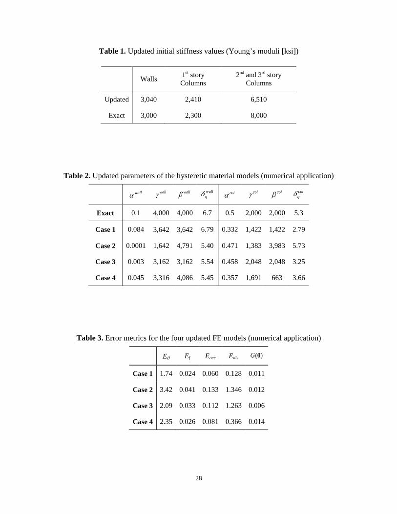
Table 2. Updated parameters of the hysteretic material models (numerical application)

wallα wallγ

wallβ wallηδ colα colγ colβ col

ηδ

Exact 0.1 4,000 4,000 6.7 0.5 2,000 2,000 5.3

Case 1 0.084 3,642 3,642 6.79 0.332 1,422 1,422 2.79

Case 2 0.0001 1,642 4,791 5.40 0.471 1,383 3,983 5.73

Case 3 0.003 3,162 3,162 5.54 0.458 2,048 2,048 3.25

Case 4 0.045 3,316 4,086 5.45 0.357 1,691 663 3.66

Table 3. Error metrics for the four updated FE models (numerical application)

Eθ Ef Eacc Edis ( )G θ

Case 1 1.74 0.024 0.060 0.128 0.011

Case 2 3.42 0.041 0.133 1.346 0.012

Case 3 2.09 0.033 0.112 1.263 0.006

Case 4 2.35 0.026 0.081 0.366 0.014

29

Table 4. Comparison of modal parameters of updated FE model and those identified from measured data

Natural Freq. [Hz] MAC [%]

Mode 1 Mode 2 Mode 1 Mode 2

Identified 16.39 39.08 99.6 98.1

Model predicted 16.39 39.08

Table 5. Updated parameters of the hysteretic material models (experimental application)

wallα wallγ

wallβ wallηδ colα colγ colβ col

ηδ

Case 1 0.058 39,918 39,918 3.49 0.399 22,790 22,790 1.90

Case 2 0.101 37,352 37,352 2.79 0.340 19,258 19,258 1.31

Table 6. Error metrics for the four updated FE models (experimental application)

Eacc Edis ( )G θ

Case 1 0.749 1.785 0.981

Case 2 0.651 1.593 1.222

Fig. 1 Test structure on the UCSD shake table

Fig. 2 Measured roof acceleration time histories during 67% and 83% Gilroy tests

10 15 20 25 30 35−2

0

2

10 15 20 25 30 35−2

0

2Acc

eler

atio

n [g

]

Time [sec]

83% Gilroy

67% Gilroy

Fig. 3 First floor displacement vs. base shear hysteretic curves during 67% and 83% Gilroy tests

Fig. 4 Nonlinear FE model of the test structure in OpenSees

−0.15 0 0.15

−200

0

200

−0.15 0 0.15

−200

0

200

Walls (Bouc-Wen)

Columns, fi rst story (Bouc-Wen)

Columns, upper stories (linear)

Beams (Rigid)

Displacement [in]

Shea

r For

ce [k

ips]

Displacement [in]

83% Gilroy 67% Gilroy

Fig. 5 Time history of the 83% Gilroy earthquake and the identified first two natural frequencies of the test structure at 17 points along this record

Fig. 6 Mode shapes of the first two longitudinal modes identified at t = 13.25 second of the 83% Gilroy test

−1

0

1

7

12

17

10 15 20 25 30 3523

31

39

Time [sec]

Freq

uenc

y [H

z]

Mode 1

Mode 2

Mode 1 Mode 2

Acc

eler

atio

n [g

]

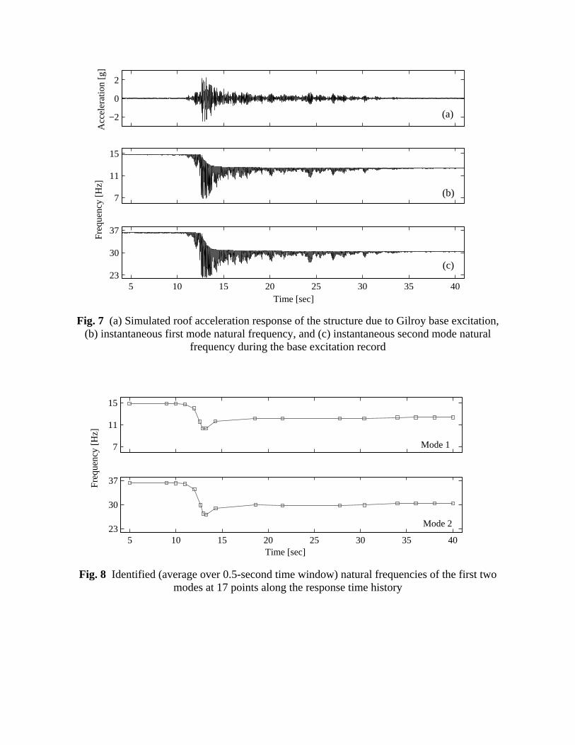
Fig. 7 (a) Simulated roof acceleration response of the structure due to Gilroy base excitation, (b) instantaneous first mode natural frequency, and (c) instantaneous second mode natural

frequency during the base excitation record

Fig. 8 Identified (average over 0.5-second time window) natural frequencies of the first two modes at 17 points along the response time history

−2

0

2

7

11

15

5 10 15 20 25 30 35 4023

30

37

7

11

15

5 10 15 20 25 30 35 4023

30

37

(a)

(b)

(c)

Acc

eler

atio

n [g

] Fr

eque

ncy

[Hz]

Time [sec]

Time [sec]

Freq

uenc

y [H

z]

Mode 1

Mode 2

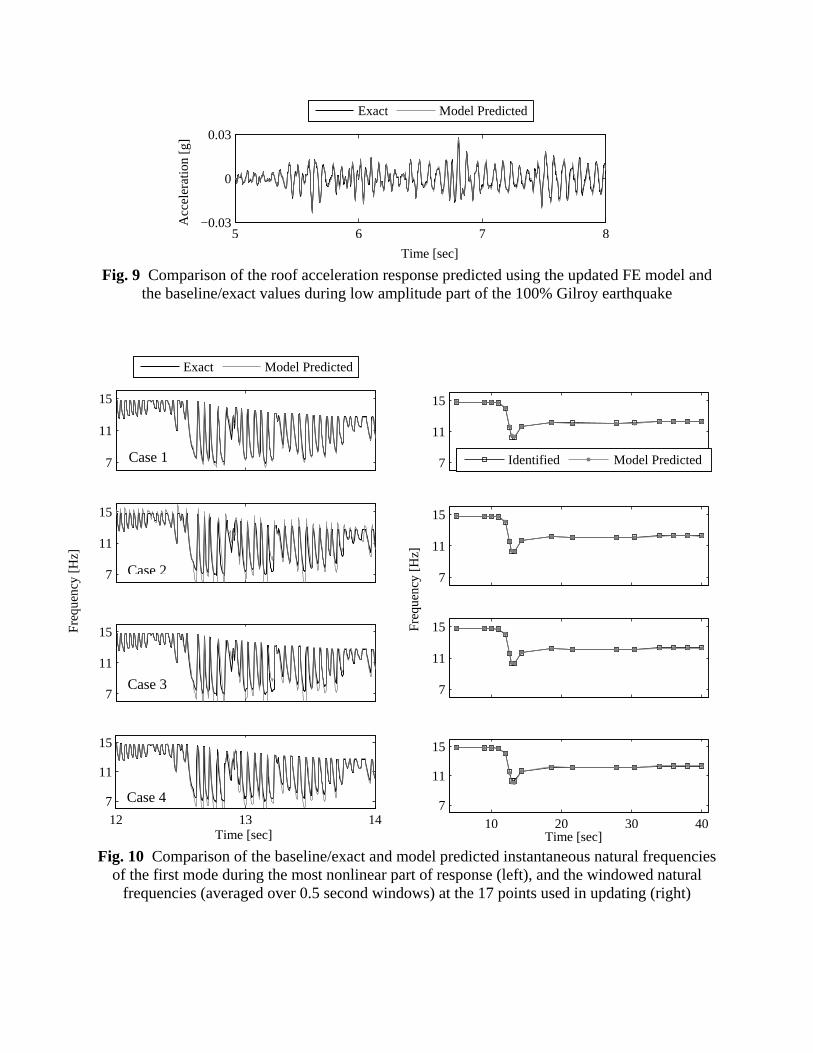
Fig. 9 Comparison of the roof acceleration response predicted using the updated FE model and the baseline/exact values during low amplitude part of the 100% Gilroy earthquake

Fig. 10 Comparison of the baseline/exact and model predicted instantaneous natural frequencies of the first mode during the most nonlinear part of response (left), and the windowed natural

frequencies (averaged over 0.5 second windows) at the 17 points used in updating (right)

5 6 7 8−0.03

0

0.03

Exact Model Predicted

7

11

15

Exact Model Predicted

7

11

15

Identified Model Predicted

7

11

15

7

11

15

7

11

15

7

11

15

12 13 147

11

15

10 20 30 407

11

15

Time [sec] Time [sec]

Time [sec]

Acc

eler

atio

n [g

]

Freq

uenc

y [H

z]

Case 1

Case 2

Case 3

Case 4

Freq

uenc

y [H

z]

Fig. 11 Comparison of the baseline/exact and model predicted roof acceleration (left) and first story displacements (right) responses during the most nonlinear part of response

−3

0

3

Exact Model Predicted

−0.2

0

0.2

−3

0

3

−0.2

0

0.2

−3

0

3

−0.2

0

0.2

12 13 14 15−3

0

3

−0.2

0

0.2

Dis

plac

emen

t [in

]

Acc

eler

atio

n [g

]

Time [sec] Time [sec]

Case 1

Case 2

Case 3

Case 4

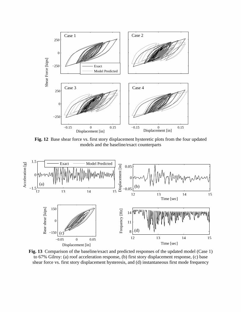
Fig. 12 Base shear force vs. first story displacement hysteretic plots from the four updated models and the baseline/exact counterparts

Fig. 13 Comparison of the baseline/exact and predicted responses of the updated model (Case 1) to 67% Gilroy: (a) roof acceleration response, (b) first story displacement response, (c) base shear force vs. first story displacement hysteresis, and (d) instantaneous first mode frequency

−250

0

250

Exact

Model Predicted

−0.15 0 0.15

−250

0

250

−0.15 0 0.15

12 13 14 15−1.5

0

1.5

Exact Model Predicted

12 13 14 15−0.05

0

0.05

−0.05 0 0.05

−150

0

150

12 13 14 15

8

11

14

(a) (b)

(c) (d)

Time [sec]

Time [sec] Displacement [in]

Acc

eler

atio

n [g

]

Dis

plac

emen

t [in

]

Bas

e sh

ear [

kips

]

Freq

uenc

y [H

z]

Displacement [in] Displacement [in]

Shea

r For

ce [k

ips]

Case 1 Case 2

Case 3 Case 4

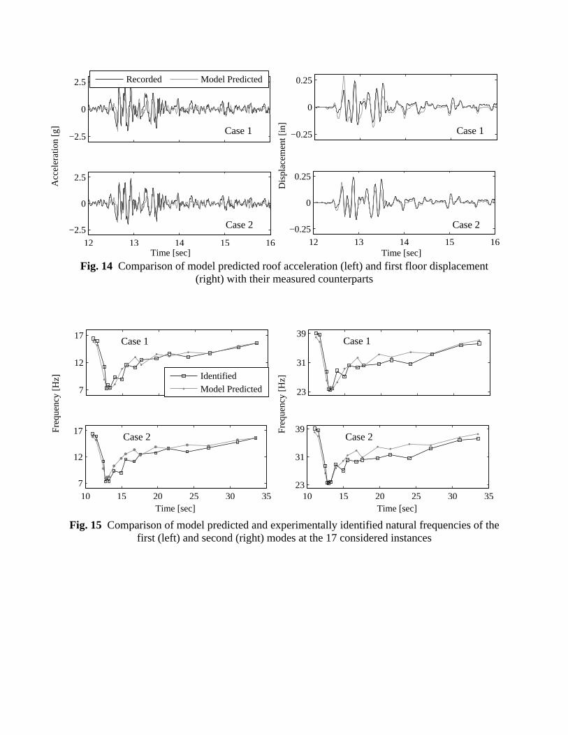
Fig. 14 Comparison of model predicted roof acceleration (left) and first floor displacement (right) with their measured counterparts

Fig. 15 Comparison of model predicted and experimentally identified natural frequencies of the first (left) and second (right) modes at the 17 considered instances

−2.5

0

2.5

Recorded Model Predicted

−0.25

0

0.25

12 13 14 15 16

−2.5

0

2.5

12 13 14 15 16−0.25

0

0.25

7

12

17

Identified

Model Predicted 23

31

39

10 15 20 25 30 35

7

12

17

10 15 20 25 30 3523

31

39

Case 1

Case 2

Time [sec] Time [sec]

Case 1

Case 2

Dis

plac

emen

t [in

]

Acc

eler

atio

n [g

] Fr

eque

ncy

[Hz]

Freq

uenc

y [H

z]

Time [sec] Time [sec]

Case 2

Case 1

Case 1

Case 2

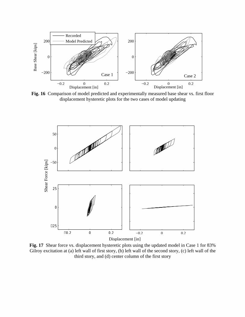
Fig. 16 Comparison of model predicted and experimentally measured base shear vs. first floor displacement hysteretic plots for the two cases of model updating

Fig. 17 Shear force vs. displacement hysteretic plots using the updated model in Case 1 for 83% Gilroy excitation at (a) left wall of first story, (b) left wall of the second story, (c) left wall of the

third story, and (d) center column of the first story

−0.2 0 0.2

−200

0

200

Recorded

Model Predicted

−0.2 0 0.2

−200

0

200

−50

0

50

−0.2 0 0.2

−25

0

25

−0.2 0 0.2

Bas

e Sh

ear [

kips

]

Case 1 Case 2

Displacement [in] Displacement [in]

Displacement [in]

Shea

r For

ce [k

ips]

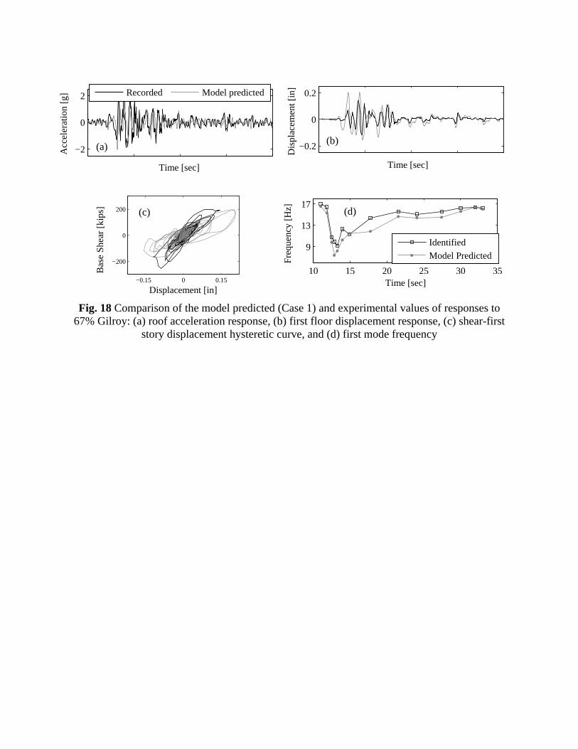
Fig. 18 Comparison of the model predicted (Case 1) and experimental values of responses to 67% Gilroy: (a) roof acceleration response, (b) first floor displacement response, (c) shear-first

story displacement hysteretic curve, and (d) first mode frequency

−2

0

2

Recorded Model predicted

−0.2

0

0.2

−0.15 0 0.15

−200

0

200

10 15 20 25 30 35

9

13

17

Identified

Model Predicted

(a) (b)

(c) (d)

Time [sec]

Time [sec] Displacement [in]

Acc

eler

atio

n [g

]

Dis

plac

emen

t [in

]

Bas

e Sh

ear [

kips

]

Freq

uenc

y [H

z]

Time [sec]