Nonlinear SISO System Identification Applied to the Series System Power-Driver, DC-Motor and Propeller José Fort Ruiz Thesis to obtain the Master of Science Degree in Electrical and Computer Engineering Supervisor: Professor José António da Cruz Pinto Gaspar Examination Committee Chairperson: Professor João Fernando Cardoso Silva Sequeira Supervisor: Professor José António da Cruz Pinto Gaspar Member: Professor Rita Maria Mendes de Almeida Correia da Cunha June 2015
Transcript
Nonlinear SISO System Identification
Applied to the Series System
Power-Driver, DC-Motor and Propeller
José Fort Ruiz
Thesis to obtain the Master of Science Degree in
Electrical and Computer Engineering
Supervisor: Professor José António da Cruz Pinto Gaspar
Examination Committee
Chairperson: Professor João Fernando Cardoso Silva Sequeira
Supervisor: Professor José António da Cruz Pinto Gaspar
Member: Professor Rita Maria Mendes de Almeida Correia da Cunha
June 2015
Resumo
Nesta tese propõe-se uma metodologia dos mínimos quadradospara estimar os parâmetros de
um sistema não linear composto por um amplificador de potência (power driver), um Motor-DC
e uma hélice. A entrada do sistema é a tensão da referência e a saída é a velocidade da rotação
das pás da hélice.
Duas parametrizações são consideradas. As parametrizações diferem se o principal efeito
é associado (i) à hélice ou (ii) ao amplificador de potência. Para além da proposta de um
processo de modelação do sistema por estimação paramétrica, é também realizada uma análise
de sensibilidade do processo de estimação.
A análise de sensibilidade do processo de estimação é baseada na adição de ruído Gaussiano
sobre a resposta do sistema simulado e consequente observação de efeito sobre os parâmetros
recalculados com base nos dados com ruído.
A metodologia de modelação é aplicada sobre dados adquiridos em um sistema real. Os
resultados da estimação são utilizados para comparar os efeitos não lineares do driver de potên-
cia e da hélice. A análise de sensibilidade é realizada sobreo modelo que melhor representa o
sistema real.
ii
Abstract
In this thesis is proposed a least squares methodology to estimate the parameters of a non-linear
system composed by one Power Driver, one DC Motor and one Propeller. The input of the
system is the reference power and the output is the rotation speed of the two blades propeller.
Two parametrizations are considered. The parametrizations differ whether the main non
linear effect is associated to (i) the propeller, or (ii) thepower driver. In addition, the estimation
process is assessed based in a sensitivity analysis. This analysis is performed using a numerical
procedure where Gaussian noise is added to the response of a simulated system, and then the
system parameters are recomputed based in the noisy data.
Data acquired from a real system is used to test the parameters estimation methodology.
Then, the estimation results are used to assess whether the real system has a non-linear effect
more, or lesser, severe in the power driving or the propeller. The sensitive analysis is performed
The motivation for this work comes from an EEC course on Real Time Distributed Control
Systems lectured by Professor Carlos Silvestre [5]. This course involves, among other tasks,
regulating the height of a levitating ball enclosed in a vertical tube. The ball is actuated by a
propeller coupled to a DC motor. The reference values are sent to the motor by a dedicated
microcontroller, which also acquires ball-height measurements and interfaces to a dedicated PC
through a CAN bus.
Power driver, DC motor and propeller (PMP), form the actuation component of the complete
setup and is the subsystem to be identified in this work. The propeller introduces by itself a
nonlinear (quadratic) relationship between the motor spinning speed and the propelling force.
The power driver is composed by one single MOSFET transistor, working in saturation and
pulsed by a PWM signal, hence adding another nonlinear component to the system. The purpose
of our work is to identify the PMP as a continuous system, using an approximate model. We
include the non-linear terms in the PMP model in order to obtain a more accurate real system
identification.
Given that the main motivation of this work comes from a didactic setup, and the work has
the purpose of continuing to serve didactic purposes, we seek to propose and validate simple
identification methodologies. As noted in work [1], entitled Nonlinear system identification is
simple, knowing the state of a continuous system and its derivatives as functions of the control
and output variables, is equivalent to know the system itself. Commonly, one has sensors giving
observations of the state but not of its time derivatives. Inorder to identify the system, one can
than follow a system discretization approach [2] or, more recently, try to estimate directly the
derivatives using filtering kernels [1, 6]. We follow the later approach, by considering simple,
non-causal, first order, difference kernels to estimate thestate derivatives.
2 Introduction
More in detail, the thesis encompasses the proposal of a model for the PMP system, the
identification of the parameters of the model given real data, and a sensibility analysis of the
identification methodology.
We start by modeling each of the three subsystems composing the PMP system using
physics. Then the partial models are combined. The resulting model has the form of a non-
linear differential equation, having as input the motor reference voltage and as state, and output,
the rotation speed of the propeller. The partial models introduce non linear components into the
complete system model.
Having obtained the non linear model, we introduce one methodology to estimate the pa-
rameters of the model. The methodology is based in least squares, comparing real-system re-
sponses with model-based responses. Real system data encompasses input, state and derivative
state signals. This information is obtained with a data acquisition card and signal pre-processing
as, e.g., a Schmitt-Trigger to attenuate noise. The data acquired allows fitting various models,
more precisely various numbers of parameters, indicating different combinations of the various
non-linearities, and therefore assessing the relative importance of the non-linearities.
Finally, a sensibility analysis, based on noise added to thesensor and re-estimation of pa-
rameters, considering the best fit model, allows assessing the validity of the methodology.
The thesis follows the following structure: Chapter 2 introduces the system studied in this
master thesis. We divide the complete system into three subsystems and detail their non linear
components. This chapter ends with the problem formulationon non linear systems identi-
fication. Chapter 3 presents the identification methodologybased in the estimation of model
parameters. Non-linear terms are included to represent accurately the real system in a least
squares sense. Chapter 4 details the experiments conductedin this dissertation. This chapter
is composed by two main sections. The first one identifies the PMP real model. The second
section assesses the effect of sensor noise into the identification of the system. Chapter 5 sum-
marizes the results obtained along the thesis, indicates alternative ideas for non-linear system
identification and presents suggestions for future work.
Chapter 2
Non-Linear SISO System
2.1 Setup Power-Motor-Propeller
In this section is detailed the nonlinear system consideredin this thesis. The system is composed
of three main subsystems connected in series: Power-Driver, DC-Motor and Propeller. In the
following the acronym PMP is used to indicate the complete system. Figure 2.1 shows the
whole system.
Figure 2.1: Photograph and diagram of the levitating ball setup.
One central objective of this thesis is the identification ofthe PMP model. We follow a
parametric model based approach. We start by introducing the parametric model.
The aim of PMP system is to keep one ball inside a tube in a wanted height. To get the ball
flying we use the propeller driven by a DC-Motor through a shaft. The DC-Motor provides the
torque to make the propeller spin and the latter keeps the ball in the air. The DC-Motor is driven
by the current provided by the switched ON/OFF MOSFET. The MOSFET amplifies the power
of PWM signal provided by a micro controller.
4 Non-Linear SISO System
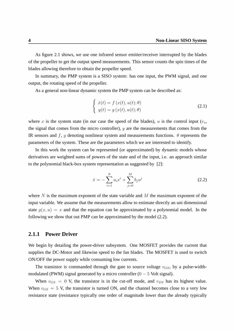
As figure 2.1 shows, we use one infrared sensor emitter/receiver interrupted by the blades
of the propeller to get the output speed measurements. This sensor counts the spin times of the
blades allowing therefore to obtain the propeller speed.
In summary, the PMP system is a SISO system: has one input, thePWM signal, and one
output, the rotating speed of the propeller.
As a general non-linear dynamic system the PMP system can be described as:
x(t) = f (x(t), u(t); θ)
y(t) = g (x(t), u(t); θ)(2.1)
wherex is the system state (in our case the speed of the blades),u is the control input (vs,
the signal that comes from the micro controller),y are the measurements that comes from the
IR sensors andf , g denoting nonlinear system and measurements functions.θ represents the
parameters of the system. These are the parameters which we are interested to identify.
In this work the system can be represented (or approximated)by dynamic models whose
derivatives are weighted sums of powers of the state and of the input, i.e. an approach similar
to the polynomial black-box system representation as suggested by [2]:
x = −
N∑
i=1
aixi +
M∑
j=0
bjuj (2.2)
whereN is the maximum exponent of the state variable andM the maximum exponent of the
input variable. We assume that the measurements allow to estimate directly an uni dimensional
stateg(x, u) = x and that the equation can be approximated by a polynomial model. In the
following we show that out PMP can be approximated by the model (2.2).
2.1.1 Power Driver
We begin by detailing the power-driver subsystem. One MOSFET provides the current that
supplies the DC-Motor and likewise speed to the fan blades. The MOSFET is used to switch
ON/OFF the power supply while consuming low currents.
The transistor is commanded through the gate to source voltage vGS, by a pulse-width-
modulated (PWM) signal generated by a micro controller (0− 5 Volt signal).
When vGS = 0 V, the transistor is in the cut-off mode, andvDS has its highest value.
WhenvGS = 5 V, the transistor is turned ON, and the channel becomes closeto a very low
resistance state (resistance typically one order of magnitude lower than the already typically
2.1 Setup Power-Motor-Propeller 5
small resistance of the motor). The transition from cut-offto the ohmic mode, implies transients
wherevDS is still large and thus the MOSFET has a saturation behavior during the transient.
Assuming that the counter electromotive force is approximately zero,vcemf ≈ 0 andLa ≈ 0,
one has thatia = (VSS − vDS)/Ra. Considering transient saturation and ohmic modes, the
current of the MOSFET,ia has linear, mixed with quadratic, relationships with the gate-to-
source,vGS and drain-to-source,vDS voltages as it shows the plot in figure 2.2 [3].
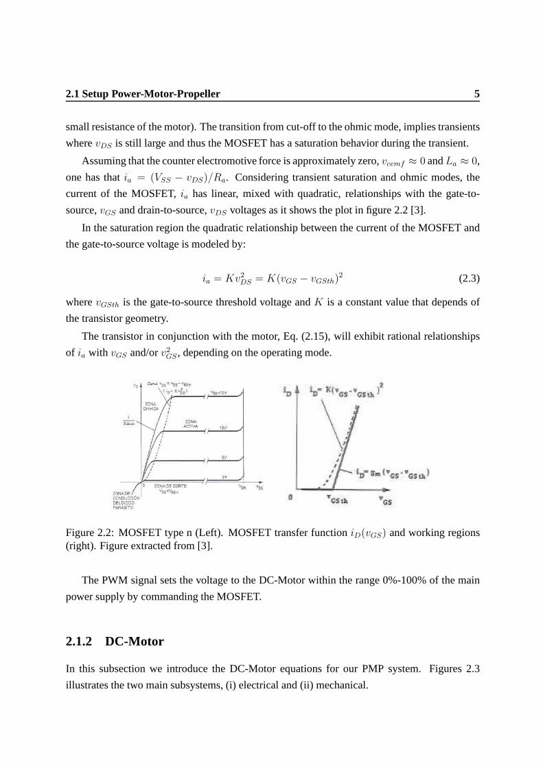
In the saturation region the quadratic relationship between the current of the MOSFET and
the gate-to-source voltage is modeled by:
ia = Kv2DS = K(vGS − vGSth)2 (2.3)
wherevGSth is the gate-to-source threshold voltage andK is a constant value that depends of
the transistor geometry.
The transistor in conjunction with the motor, Eq. (2.15), will exhibit rational relationships
of ia with vGS and/orv2GS, depending on the operating mode.
Figure 2.2: MOSFET type n (Left). MOSFET transfer functioniD(vGS) and working regions(right). Figure extracted from [3].
The PWM signal sets the voltage to the DC-Motor within the range 0%-100% of the main
power supply by commanding the MOSFET.
2.1.2 DC-Motor
In this subsection we introduce the DC-Motor equations for our PMP system. Figures 2.3
illustrates the two main subsystems, (i) electrical and (ii) mechanical.
6 Non-Linear SISO System
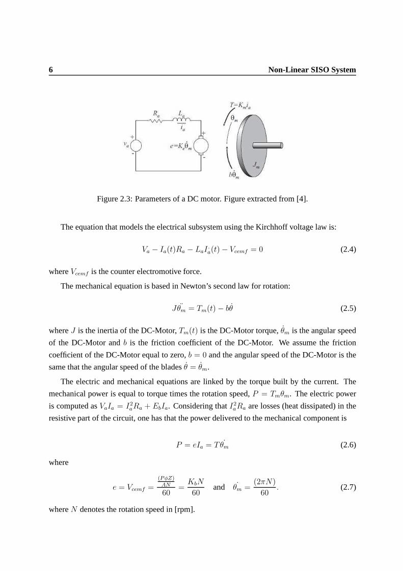
Figure 2.3: Parameters of a DC motor. Figure extracted from [4].
The equation that models the electrical subsystem using theKirchhoff voltage law is:
Va − Ia(t)Ra − LaI.a(t)− Vcemf = 0 (2.4)
whereVcemf is the counter electromotive force.
The mechanical equation is based in Newton’s second law for rotation:
Jθm = Tm(t)− bθ (2.5)
whereJ is the inertia of the DC-Motor,Tm(t) is the DC-Motor torque,θm is the angular speed
of the DC-Motor andb is the friction coefficient of the DC-Motor. We assume the friction
coefficient of the DC-Motor equal to zero,b = 0 and the angular speed of the DC-Motor is the
same that the angular speed of the bladesθ = θm.
The electric and mechanical equations are linked by the torque built by the current. The
mechanical power is equal to torque times the rotation speed, P = Tmθm. The electric power
is computed asVaIa = I2aRa + EbIa. Considering thatI2aRa are losses (heat dissipated) in the
resistive part of the circuit, one has that the power delivered to the mechanical component is
P = eIa = T ˙θm (2.6)
where
e = Vcemf =(PφZ)AN
60=
KbN
60and ˙θm =
(2πN)
60. (2.7)
whereN denotes the rotation speed in [rpm].
2.1 Setup Power-Motor-Propeller 7
Then, we have
T (t) =Kb
2πIa(t) = KmIa(t) (2.8)
having just obtained a relationship of torque with current.
Finally, the fan works due to DC motor1 and owing to the second law of Newton, the
difference on the pressure between the providing pressure of the fan and the pressure above it
(atmospheric) the ball could levitate higher or lower.
2.1.3 Propeller
The propeller is the last subsystem of the PMP model. It is theresponsible to keep the ball
in the air at a desired height. Our propeller has two blades and is connected by an axis to the
DC-Motor that provides torque to move it. The blades are modeled by:
Th(t) = −Kh1θ(t)−Kh2
θ2(t) (2.9)
where
• Th(t) is the blades torque
• Kh1 is the friction coefficient of the blades proportional to theangular speed[N.m.rad−1.s]
• Kh2 is the friction coefficient of the blades proportional to thesquare angular speed
[N.m.rad−2.s2]
• θ(t) is the angular speed of the blades.
Equation (2.9) shows the torque opposite to the torque moving the blades.
As explained before, we measure the rotation speed of the blades using one infrared sensor
(emitter/receiver) to get the output speed measurements counting the spin times of the blades.
The last subsystem is the ball-tube system where the ball is located as it could be seen in
figure 2.4. To ease (or not make it unnecessarily hard), the ball and fan will be considered like
discs.
Figure 2.4 shows the difference between the real process andour mathematical model. Pres-
suresP1 andP4 are in contact with the air so are the same as the atmospheric pressure,P2 is
the pressure from the fan andP3 is the force that makes go up or down the ball. Then, we have
1The DC-Motor used is the Graupner 500 sp which has a nominal voltage : 8.4V, No-load rpm= 32000min−1.This motor is typically used for model flight, then enough forour purpose.
8 Non-Linear SISO System
Figure 2.4: Real system propels a ball (left) while the approximate model is based in a disc(right). Figure extracted from [5].
to find the expressions that give us the pressure below the ball and the force balance in the ball.
The equation of the force balance in the ball is based in Newton’s second law:
mz(t) = A(P3 − P4)−mg (2.10)
wherem is the mass of the ball,z(t) is the vertical position in the tube,A is the area of the ball
(same as the area of an orthogonal section of the tube), andg is the gravitational acceleration.
For the pressure below the ball, we use the Bernoulli’s law. This law is valid for all the
fluids, including air, which is the case of our setup:
Pi +1
2ρv2i + gzi = Pi−1 +
1
2ρv2i−1 + gzi−1 (2.11)
In the casesi = 3 andi = 2 we can do many simplifications like assuming that air is an ideal
fluid and therefore the density and velocity are the same in both sides owing to the short length
of the tube. We can assume also that the ball is represented bya thin disk, i.e. Z3 = Z2.
After the simplifications, one obtainsP3 = P2. The next step is to find the valueP2. From
the assumption that the ball can be represented as a disc, we obtainP2 by considering that the
propeller produces pressure as a force divided the cylinderarea:
P2 = P1 +F (t)
A(2.12)
2.1 Setup Power-Motor-Propeller 9
The equation of the force generated by the fan is:
F (t) =1
4ρnpc(Ω(t)R)2Raoθo (2.13)
wherenp is the number of blades in the fan,c is the width of the blades,Ω is the angular velocity,
R is the fan radius,θo is the blade incident angle, andao is the aerodynamics constant.
Noting thatΩ is the variable of interest, a much simpler model can be proposed:
F (t) = Kh(t)Ω2(t) (2.14)
whereKh is a constant to be determined experimentally.
2.1.4 Complete PMP Model
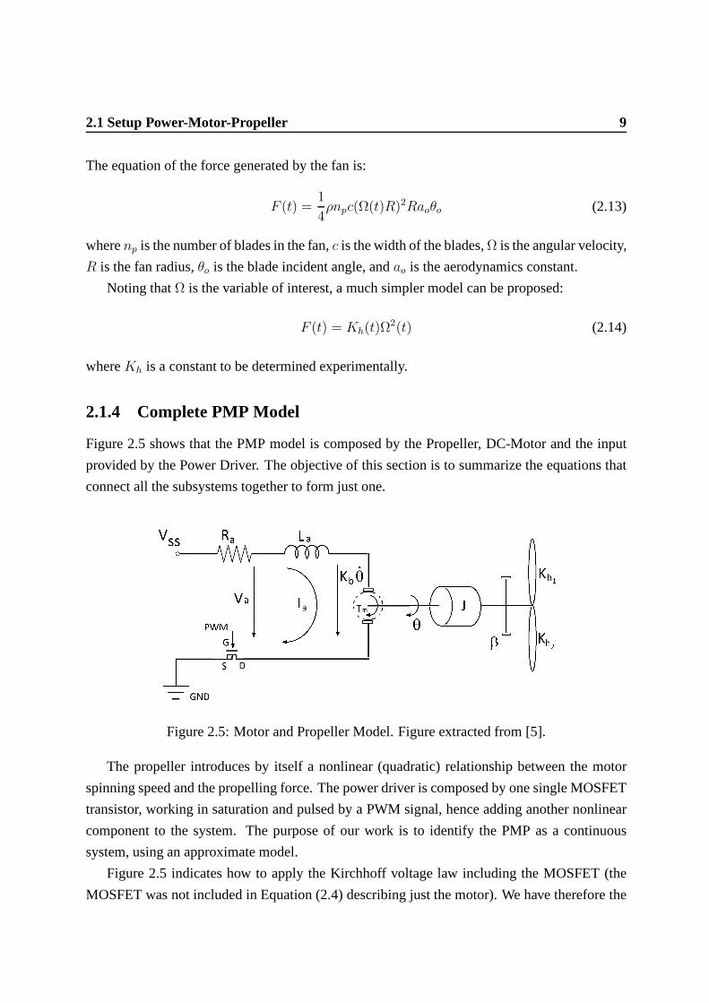
Figure 2.5 shows that the PMP model is composed by the Propeller, DC-Motor and the input
provided by the Power Driver. The objective of this section is to summarize the equations that
connect all the subsystems together to form just one.
Figure 2.5: Motor and Propeller Model. Figure extracted from [5].
The propeller introduces by itself a nonlinear (quadratic)relationship between the motor
spinning speed and the propelling force. The power driver iscomposed by one single MOSFET
transistor, working in saturation and pulsed by a PWM signal, hence adding another nonlinear
component to the system. The purpose of our work is to identify the PMP as a continuous
system, using an approximate model.
Figure 2.5 indicates how to apply the Kirchhoff voltage law including the MOSFET (the
MOSFET was not included in Equation (2.4) describing just the motor). We have therefore the
10 Non-Linear SISO System
following equation which relates the power driver with DC-Motor:
VSS = RaIa + La
d
dtia + vcemf + vDS (2.15)
whereVSS is the power supply,Vcemf is counter electromotive force andvDS is the voltage
coming from the MOSFET.
Equation (2.15) shows that the MOSFET voltage generates currentIa. Next we restate that
currentIa implies motor torqueTm. Equations (2.6) and (2.7) allow connecting the axis with
the DC-Motor in function with the counter electromotive force as follows:
Tm(t) = Kb/2πIa(t) = KmIa(t) . (2.16)
In summary, the MOSFET voltage implies motor torque. Next weindicate the main non-
linearity in this process.
The first non-linearity that appears in our system is locatedin the Power Driver, more pre-
cisely on the MOSFET. Equation (2.3) shows a non-linear, quadratic, behavior between the
command of the MOSFET, the PWM signal, and the current driventhrough the MOSFET.
In order to characterize the effect of the PWM average value and, more precisely, its pro-
gramming valuevref , used in the micro controller software2, to the torque generated by the
motor, Tm, which is proportional to the current,Tm = Kmia, we use the simplified model
following the structure of the equation (2.2) related to theinput variable and considering the
quadratic relationship ofia with vref suggested by the MOSFET:
Tm = β0 + β1vref + β2v2ref (2.17)
whereβ0, β1, β2 are constant parameters.
Having characterized the system fromvref to Tm, we just have to add the propeller to com-
plete the PMP model. The blades of the propeller introduce anopposite torque,Th, whose
balance withTm describe in essence the rotation dynamics of the system. Thepropeller intro-
duces a second non-linearity into the PMP model.
The second non linearity of the PMP system appears on the dynamics between the DC-
Motor and fan, more precisely owing to the friction blades with the air when they try to move
is modeled by the equation (2.9). This equation is related with the output variableθ, so we just
have to show the simplified model takingw = θ, α1 = Kh1andα2 = Kh2
and the new equation
2There is a linear relationship between the PWM programming values,vref ranging0 · · · 255, and the average
value of the PWM signal,∫ t+T
tvGS(t)dt/T , ranging0 · · · 5 V.
2.1 Setup Power-Motor-Propeller 11
is:
Th = α1ω + α2ω2 . (2.18)
Now we just need the last balance to connect the blades to our system. Taking equation
(2.17) we have:
Jθ(t) = Tm(t)− Th(t) (2.19)
whereTm is the torque of the DC motor andTh is the opposite torque of the blades. Then
Finally, putting together all the equations we have the following general model:
x+ a1x+ a2x2 = b0 + b1u+ b2u
2 (2.20)
whereai = αi/J , u = vref , x = ω andbi = βi/J .
As referred in the beginning of the chapter, the PMP model is polynomial in the inputs and
in the state. Equation (2.20) is a particular case of the general polynomial equation (2.2). This
model will allow us to know the system itself by observing thecontrol and state variables, and
estimating the state derivative.
2.1.5 Problem Formulation
Non linear systems present some formulation problems and identification difficulties that linear
systems do not. One of the aspects of non linear systems is that one cannot use the superposition
principle and use it to obtain simple solutions.
In some cases nonlinear systems are approached as linear systems. The way to do it is
by finding the work region and transforming this (limited) region into a linear system. It is
important to compare and verify if the responses are similarto the approximation. If they are,
then the identified model can be used to represent the real system. This approach can be used
for relatively simple systems3.
Fortunately, in our PMP setup the most significant effects ofthe non linear components can
be observed easily with a sensor measuring the propeller rotation speed. In the next chapter
will introduce two different identification methodologiesbased in equation (2.2). As previously
mentioned, the didactic application of the system considered in this thesis indicate using sim-
3Counter examples include chaotic systems in which it is impossible to predict what will happen. For example,weather forecast models require using large numbers of variables due to covering large areas, while encompassingmany complex interactions within the covered areas. As it isimpossible having one sensor per variable per placeof interest, weather forecast is still, nowadays, frequently imprecise.
12 Non-Linear SISO System
ple models. We will take just the minimum parameters to describe the most significant non
linearities.
Chapter 3
Identification Methodology
In this section we use a least squares formulation to estimate the parameters of the model pro-
posed for the series system, power-driver, DC-Motor and propeller (2.20).
3.1 Data Acquisition
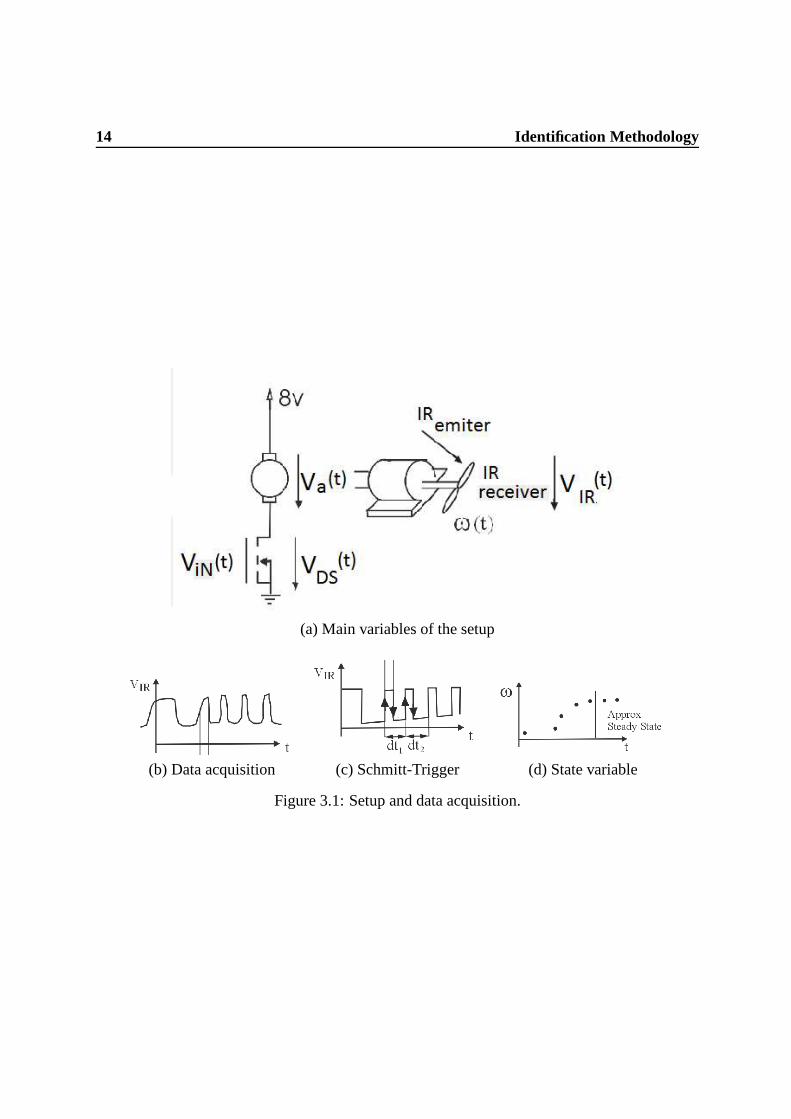
Figure 3.1 shows the setup of the hardware and the pre-processing associated to data acquisi-
tion. Figure 3.1(a) shows the Power-Motor-Propeller system and the variables that model his
behavior. There are two main variables of interest, namely the rotation speed,ω and the infrared
voltageVIR.
We use one infrared emitter and one receiver to count the number of times per second the
two blades pass and cut the infrared light path. When the blade cut the light path,VIR gets its
maximum value. Then, to get the rotation speed is just neededto be counted the blades twice
having in mind the time spent to do it. This is measured as timebetween two peeks onVIR.
The real signal is not as clean as shown in the figure 3.1. It hasassociated sudden ON/OFF
changes of the MOSFET which disturbs the ground voltage. Themost effective solution to this
problem is to introduce a Schmitt-Trigger. It is an active circuit which converts an analog input
signal to a digital output signal. In the non-inverting configuration, when the input is higher
than a certain chosen threshold, the output is high. When theinput is below a different (lower)
chosen threshold, the output is low, and when the input is between the two levels, the output
retains its value.
14 Identification Methodology
(a) Main variables of the setup
(b) Data acquisition (c) Schmitt-Trigger (d) State variable
Figure 3.1: Setup and data acquisition.
3.2 Model fit 15
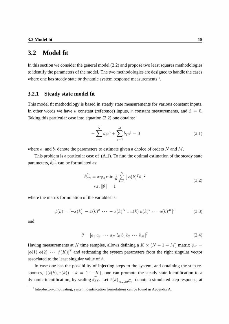
3.2 Model fit
In this section we consider the general model (2.2) and propose two least squares methodologies
to identify the parameters of the model. The two methodologies are designed to handle the cases
where one has steady state or dynamic system response measurements1.
3.2.1 Steady state model fit
This model fit methodology is based in steady state measurements for various constant inputs.
In other words we haveu constant (reference) inputs,x constant measurements, andx = 0.
Taking this particular case into equation (2.2) one obtains:
−
N∑
i=1
aixi +
M∑
j=0
bjuj = 0 (3.1)
whereai andbi denote the parameters to estimate given a choice of ordersN andM .
This problem is a particular case of (A.1). To find the optimalestimation of the steady state
Having measurements atK time samples, allows defining aK × (N + 1 + M) matrixφK =
[φ(1) φ(2) · · · φ(K)]T and estimating the system parameters from the right singular vector
associated to the least singular value ofφ.
In case one has the possibility of injecting steps to the system, and obtaining the step re-
sponses,(t(k), x(k)) : k = 1 · · ·K, one can promote the steady-state identification to a
dynamic identification, by scalingθSS. Let x(k)|u∞,αθSS .denote a simulated step response, at
1Introductory, motivating, system identification formulations can be found in Appendix A.
16 Identification Methodology
time tk, to a step input with the steady state valueu∞, considering the scaled parametersαθSS.
Then one can write another (nonlinear) least squares problem to find the scaling factorα:
α∗ = argαmin
K∑
k=1
∣∣∣x(k)− x(k)|u∞,αθSS
∣∣∣2
. (3.5)
This problem can be solved having one single sample(t(k), x(k)), but the accuracy of the so-
lution benefits of using as many as possible data samples. This nonlinear optimization problem
requires simulation and a non trivial optimization routineas the Matlab’sfminsearch. In
the next section, we see that in case one has derivative estimates, then the problem is much
simplified.
3.2.2 Dynamic model fit
When one has dynamic responses to generic (known) inputs, not necessarily just the step re-
sponses, and has a method to observe or estimate the derivatives, then it is possible to estimate
directly the steady-state system parameters and its globalscaling [1, 6].
In the following we consider a very simple, non-causal, firstorder, difference kernel, for
low noise signals. We consider the derivative approximation:
ˆx(k) =x(k + 1)− x(k − 1)
t(k + 1)− t(k − 1)(3.6)
wheret(k+1) andt(k− 1) denote the sampling times corresponding to the states, observed by
a sensor,x(k + 1) andx(k − 1).
Now we can estimate all the parameters using an unconstrained least squares approach:
θd = argθ min1
K
K∑
k=1
[ ˆx(k)− φ(k)T θ ]2 (3.7)
where the parametersθ are defined as before, but the measurementsφ are not restricted to
the steady state values, i.e.φ includes transient measurements. Then, applying the matrix
formulation (see Appendix A) the estimate of the parametersis simply obtained by a pseudo-
inverse, taking a particular case of the equation (A.12):
θd = (φTKφK)
−1φTKdX (3.8)
3.3 Summary of the Parametric Fitting Method 17
wheredX = [ˆx(1) ˆx(2) · · · ˆx(K)]T .
3.3 Summary of the Parametric Fitting Method
In this dissertation we consider two different ways to represent our system. In the first repre-
sentation we have parametersa1, a2, b0 andb1 hence giving more importance to non linearity
on the output side (Fan):
x+ a1x+ a2x2 = b0 + b1u (3.9)
In the second representation we assumea2 = 0 andb2 6= 0 hence giving relevance to the input
side or Power Driver
x+ a1x = b0 + b1u+ b2u2 (3.10)
Having specialized the two models, (3.9) and (3.10), we discuss now the minimum number
of input steps necessary for the least squares estimation methodology.
In our case, two steps are enough. To use the least squares estimation is mandatory to have
the matrixφk with complete rank. The definition of a complete rank matrix isA ∈ Mm×n is
a complete rank matrix ifrank(A) = minm,n.
We have to obtain the rank ofφk equal to the number of columns, asφk has lesser columns
than rows. In our case, the rank has to be equal to 4.
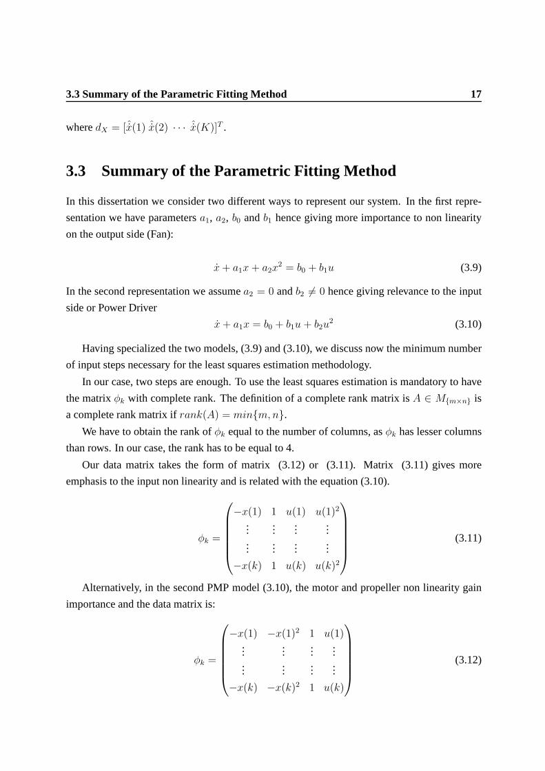
Our data matrix takes the form of matrix (3.12) or (3.11). Matrix (3.11) gives more
emphasis to the input non linearity and is related with the equation (3.10).
φk =
−x(1) 1 u(1) u(1)2
......
......
......
......
−x(k) 1 u(k) u(k)2
(3.11)
Alternatively, in the second PMP model (3.10), the motor andpropeller non linearity gain
importance and the data matrix is:
φk =
−x(1) −x(1)2 1 u(1)...
......
......
......
...
−x(k) −x(k)2 1 u(k)
(3.12)
18 Identification Methodology
Given the data matrices we can compute the system parametersusing a pseudo-inverse:
θd = (φTKφK)
−1φTKdX (3.13)
wheredX is a vector with the data related to derivative state in each sample time.
In the following paragraphs is shown that to identify model (3.9) one step is enough and in
the case of the model (3.10) one needs two steps.
Starting with case (3.9), as referred earlier, we need a matrix with all the columns linearly
independent. The column of ones and the input columns do not change. On the contrary, the
output based columns have transient values till reaching the steady states. We can see that in
just two samples one obtains a non linear combination of the others columns.
The column of ones is linearly independent owing to its constant value. Is needed one step
to be linearly independent from the input step columns owingto the change in his values. In the
case regarding to the output values is easier owing to its transient behavior.
Following the same principle, it could be explained the input case, the difference is that this
column just changes when we add another step in our simulation. Then, the critical situation to
have a complete rank in our matrix are the input columns.
In the case of the model (3.10) the higher power of the termb2u2 forces us to increment
the number of the steps applied. During the first step the columns of simple input are linear
independent. In that way, through the second one is the squared term who is linear independent.
The conclusion is that the minimum number of steps is equal tothe maximum power of the
right side of our equation number.
In summary, in the case of model (3.10) are needed two step responses and in the case of
model (3.9) is needed just one step response.
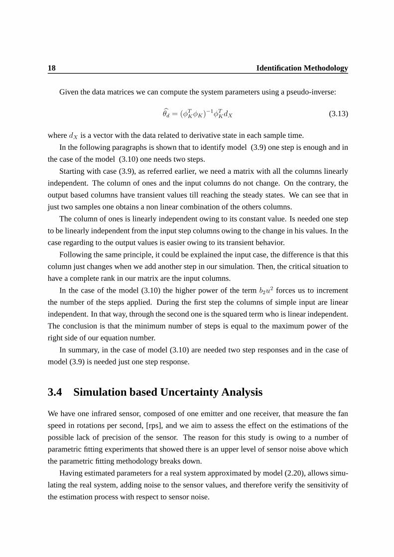
3.4 Simulation based Uncertainty Analysis
We have one infrared sensor, composed of one emitter and one receiver, that measure the fan
speed in rotations per second, [rps], and we aim to assess theeffect on the estimations of the
possible lack of precision of the sensor. The reason for thisstudy is owing to a number of
parametric fitting experiments that showed there is an upperlevel of sensor noise above which
the parametric fitting methodology breaks down.
Having estimated parameters for a real system approximatedby model (2.20), allows simu-
lating the real system, adding noise to the sensor values, and therefore verify the sensitivity of
the estimation process with respect to sensor noise.
3.4 Simulation based Uncertainty Analysis 19
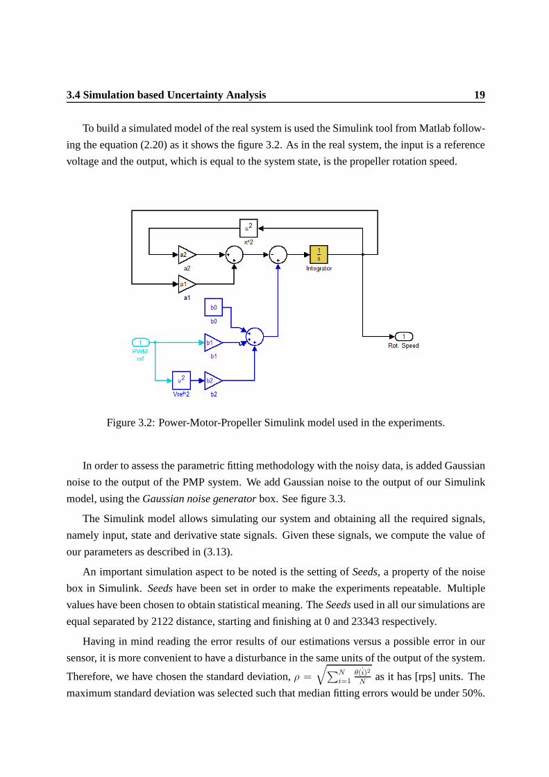
To build a simulated model of the real system is used the Simulink tool from Matlab follow-
ing the equation (2.20) as it shows the figure 3.2. As in the real system, the input is a reference
voltage and the output, which is equal to the system state, isthe propeller rotation speed.
Figure 3.2: Power-Motor-Propeller Simulink model used in the experiments.
In order to assess the parametric fitting methodology with the noisy data, is added Gaussian
noise to the output of the PMP system. We add Gaussian noise tothe output of our Simulink
model, using theGaussian noise generatorbox. See figure 3.3.
The Simulink model allows simulating our system and obtaining all the required signals,
namely input, state and derivative state signals. Given these signals, we compute the value of
our parameters as described in (3.13).
An important simulation aspect to be noted is the setting ofSeeds, a property of the noise
box in Simulink. Seedshave been set in order to make the experiments repeatable. Multiple
values have been chosen to obtain statistical meaning. TheSeedsused in all our simulations are
equal separated by 2122 distance, starting and finishing at 0and 23343 respectively.
Having in mind reading the error results of our estimations versus a possible error in our
sensor, it is more convenient to have a disturbance in the same units of the output of the system.
Therefore, we have chosen the standard deviation,ρ =
√∑N
i=1
˙θ(i)2
Nas it has [rps] units. The
maximum standard deviation was selected such that median fitting errors would be under 50%.
20 Identification Methodology
Figure 3.3: Power-Motor-Propeller Simulink model with added Gaussian noise in its output.The block namedNon Linear SISO Systemis the PMP model, detailed in figure 3.2.
One way to plot fitting errors is using the Root Mean Squared Error (RMS):
RMSE =
√√√√ 1
N
N∑
i=1
(xi − xi)2 . (3.14)
wherexi is our fan speed estimator andxi is the fan speed of the real system.
Alternatively, we can use also an average of relative errors, computed per sample
E% =1
N
N∑
i=1
∣∣∣∣xi − xi
xi
∣∣∣∣× 100 (3.15)
since our measurementsxi are in essence positive, not zero, values.
Chapter 4
Experiments
4.1 Data Acquisition
The input (PWM) voltage drives a Propeller coupled to a DC motor, through a MOSFET. Fig-
ure 4.1 shows pictures of the system (see also figure 3.1 for anexplaining diagram). The
propeller lifts the ball. In this work we model the referencevoltage to the propeller rotation
speed. In order to obtain rotation speed measurements we usean infra-red LED emitter (see
figure 4.1(b)) and an infra-red receiver (see figure 4.1(c)).The blades of the propeller interrupt
the infra-red path, twice for each complete rotation, and therefore allow observing the rotation
speed by counting half the number of interruptions per second (units are therefore rotations per
second, rps).
Propeller IR rec
IR emitPropeller
IR rec
IR emit
(a) Setup (b) Bottom view (c) Side view
Figure 4.1: Detailed view of the setup. The bottom view focusthe IR emitter and the motor (b).The side view focus the IR receiver (c).
An important aspect to be considered is the possible error onthe measurements due to
22 Experiments
sampling frequency. This parameter is critical to obtain accurate data. In the following we
show that in our setup the sampling frequency is enough to cause a lesser than1% error on rps
measurements.
In order to measure speed is necessary to wait the two blades to pass in front of the IR sensor
and cut the light of the IR emitter. Considering the highest speed of the motor to bex = 200
rps, one has the maximum of400 pulses per second observed in the IR sensor. In other words,
one has a time oftp = 1/400 sec between blades andx = 1/(2tp).
All the measurements from the real system were taken by a dataacquisition board from
National Instruments. This board is able to acquire 100000 samples per second, i.e. allows a
sampling period ofTs = 10 µsec. Assuming a±Ts error in the beginning and the ending of
measuringtp, one has the maximum error ofex = 2Ts/(tp − 2Ts) ≈ 0.8%.
4.2 System Identification
In this section we identify our system by estimating the parameters of the proposed model. To
obtain these parameters we test the system with different steps. In our case we have created two
datasets encompassing (i) three or (ii) ten step responses within the range of the PWM input
signal. In addition to the step responses we compute also their derivative using a first order
difference.
As refereed in section 3.3 it will be used in this dissertation two different equations to
identify the PMP model. The equation differs depends on the importance given to each non
linearity, for this reason the model (3.9) has more importance on the non linearity of the output
(Fan) and the model (3.10) on the input (Power Driver).
4.2.1 Three Step Responses Dataset
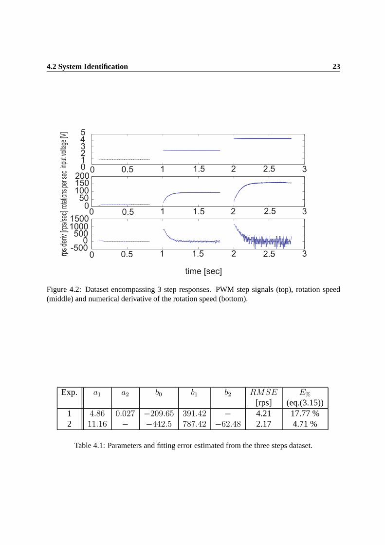
As it could be seen in figure 4.2 in the first place starting for the top we have the input values, in
the middle we observe the state information or speed rotation of the blades and derivative state
in the last place. The parameter results obtained applying the methodology are in the table 4.1.
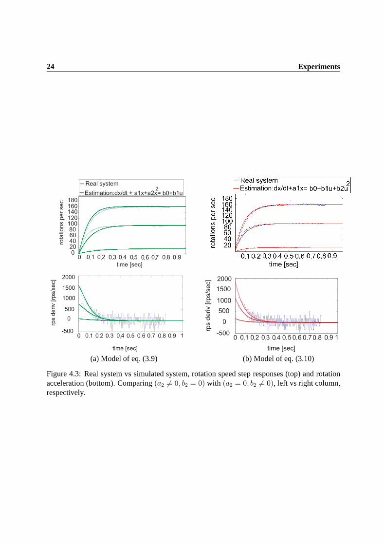
Given the estimated Power-Motor-propeller system parameters allows building a Matlab/Simulink
model and simulating step responses. This model follows thesame form of the equation (2.20).
See figure 3.2 . Figure 4.3 shows the identification results given the three steps dataset.
4.2 System Identification 23
Figure 4.2: Dataset encompassing 3 step responses. PWM stepsignals (top), rotation speed(middle) and numerical derivative of the rotation speed (bottom).
Table 4.1: Parameters and fitting error estimated from the three steps dataset.
24 Experiments
(a) Model of eq. (3.9) (b) Model of eq. (3.10)
Figure 4.3: Real system vs simulated system, rotation speedstep responses (top) and rotationacceleration (bottom). Comparing(a2 6= 0, b2 = 0) with (a2 = 0, b2 6= 0), left vs right column,respectively.
4.2 System Identification 25
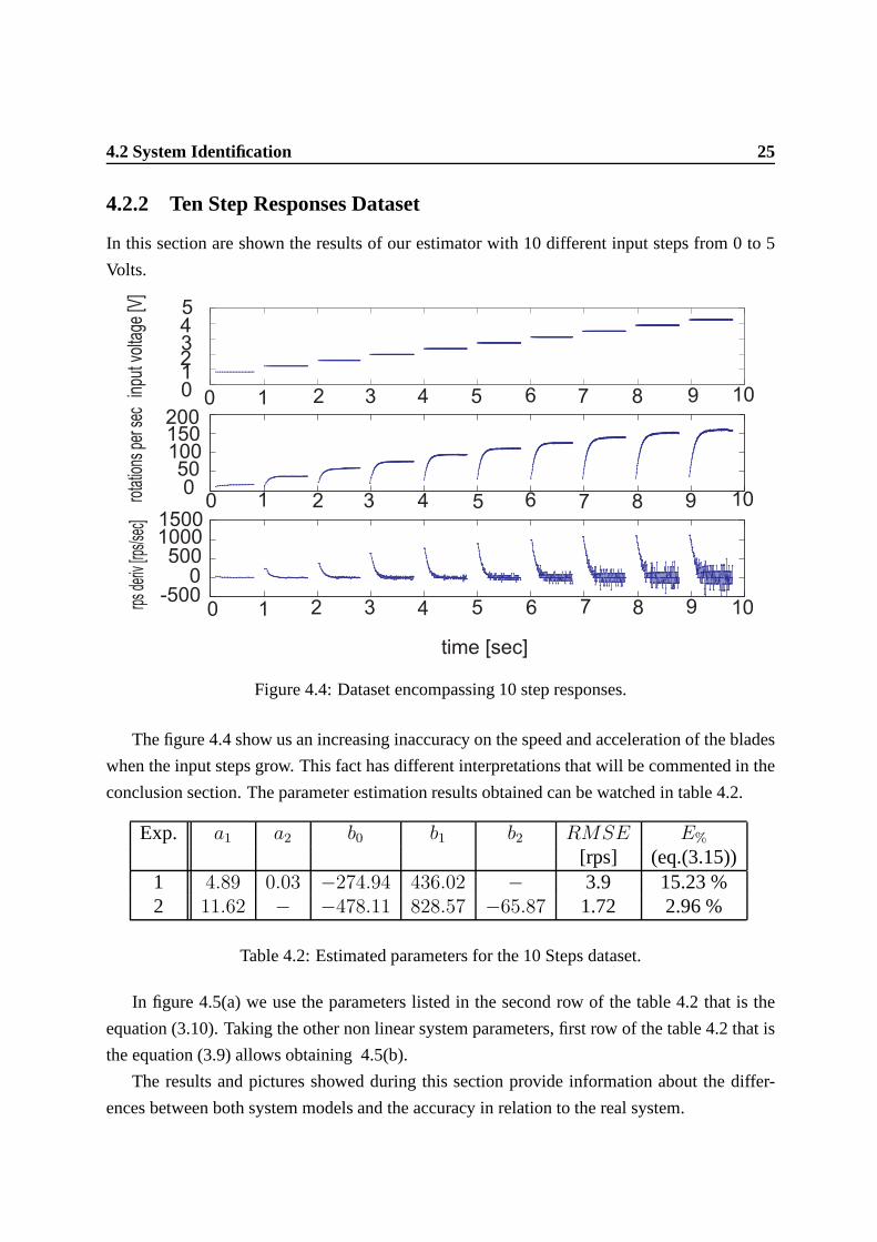
4.2.2 Ten Step Responses Dataset
In this section are shown the results of our estimator with 10different input steps from 0 to 5
Table 4.2: Estimated parameters for the 10 Steps dataset.
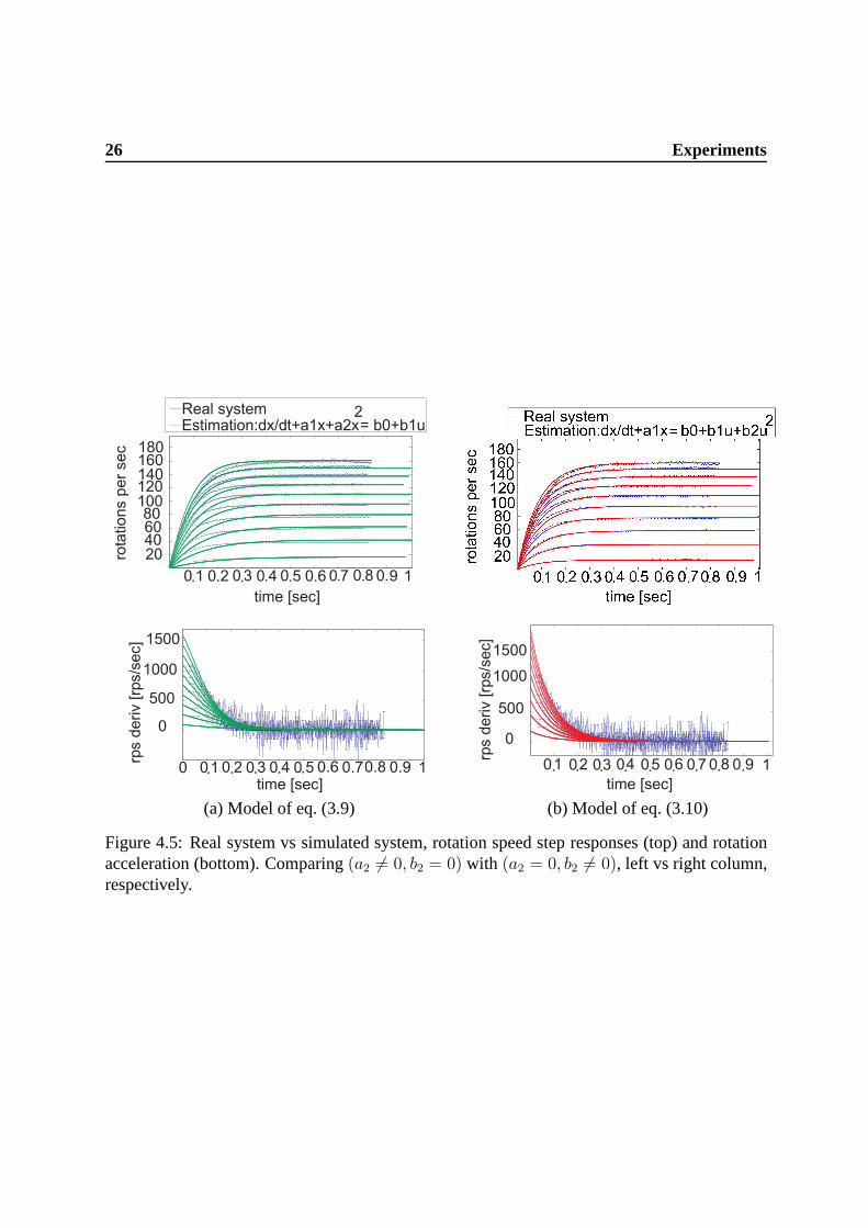
In figure 4.5(a) we use the parameters listed in the second rowof the table 4.2 that is the
equation (3.10). Taking the other non linear system parameters, first row of the table 4.2 that is
the equation (3.9) allows obtaining 4.5(b).
The results and pictures showed during this section provideinformation about the differ-
ences between both system models and the accuracy in relation to the real system.
26 Experiments
(a) Model of eq. (3.9) (b) Model of eq. (3.10)
Figure 4.5: Real system vs simulated system, rotation speedstep responses (top) and rotationacceleration (bottom). Comparing(a2 6= 0, b2 = 0) with (a2 = 0, b2 6= 0), left vs right column,respectively.
4.3 Noise Analysis 27
Results show that model (3.10) has a dynamics and steady state closer to the real system
than model (3.9).
The fitting error reasserts this fact with the data provided in the table 4.2 and 4.1 with a
significant difference between both models in terms of the RMSE and fitting error results, more
than 2 rps and 10% fitting error. Is important to watch that 10 step responses, table 4.2 provide
a little bit more accuracy than the table 4.1. For that reasonis chosen the model (3.10) 10 step
responses data to do the next experiments.
4.3 Noise Analysis
In this section we assess the system identification methodology under the effect of noise in the
sensed data. More in detail, we use the parameters estimatedin the last section to simulate the
non-linear system. The simulated system is then used to estimate again the system parameters,
given step responses of the system containing additive Gaussian noise. The global Simulink
model is shown in figure 3.3, while the detailed power-motor-propeller system is the one shown
in Fig.3.2.
The box plot representation give us a way to observe an amountof different data, as the
mean, the dispersion and symmetry of all the data obtained inthe simulations.
The results shown in figure 4.6 are generated with the aim to visualize the error in our
estimations until a 50% upper bound. We have chosen a noise limit of 6 rps.
A first observation is the relationship between the parameters and the response. More sensor
noise implies more fitting error. In another hand the resultsshow a lower fitting error for a
higher indexi in bi. For example an error b2 has a 50% fitting error instead of almost 100% of
the parameter b0.
The box-plot representation is used to watch easily the datadispersion. The box-plot pro-
vides us the following information: (i) the data dispersionbecomes higher with an increasing
noise, this feature could be seen with the box height, highermeans more dispersion, (ii) in the
most cases the dispersion is symmetric as in the highest and in the lowest values and this it
could be seen with the position of the mean red line inside thebox.
28 Experiments
0
50
100
150
200
0 1.2 2.4 3.6 4.8 6
Noise Standard Deviation [rps]
ae
rro
r [%
]1
Error in parameter a1 Error in parameter b0
0 1.2 2.4 3.6 4.8 6
Noise Standard Deviation [rps]
0
50
100
150
200
berr
or
[%]
0
0
50
100
150
200
250
berr
or
[%]
1
Error in parameter b1
0 1.2 2.4 3.6 4.8 6
Noise Standard Deviation [rps]
0
50
100
150
200b
err
or
[%]
2
Error in parameter b2
0 1.2 2.4 3.6 4.8 6
Noise Standard Deviation [rps]
0
40
80
120
160
200
0 1.2 2.4 3.6 4.8 6
Noise Standard Deviation [rps]
Err
or
[%
]
Step Responses Fitting Error vs Noise
Figure 4.6: Fitting error given Gaussian noise with variousstandard deviations (maximum 6rps). Error in parametersa1, b0, b1, b2, and error in the step response.
Chapter 5
Conclusions and Future Work
In this work has been proposed a parametric model and a methodto identify the parameters of
the power-driver, DC-motor and propeller non-linear system.
Two main aspects have been studied in this work: (i) identification of the most relevant
non-linear model components, (ii) the effect of the sensor error, i.e. the error in the rotations
per second measurements, in the accuracy of the fitted model.
The identification section shows the difference of considering the non-linearity of the power
driver vs the non-linearity introduced by the propeller. Both system models are tested with
the same data. In our case the dynamics of Power Driver (MOSFET) are more relevant than the
propeller, most probably due to the fact that it is lifting just a very-light-weighted ball. However
if the propeller would be working in different conditions, e.g. within denser fluids as water, or
higher pressures, this fact could change.
The decision of choosing a sensor is critical to the estimation. This is the second main
conclusion of this thesis. Just a small error counting the passes of the blades of the propeller has
a dramatic impact on the accuracy provided by the least squares estimation. For example, a bad
measurement of 6 rps on the 200 rps rotation speed introducesa 60% error on the estimation.
As future work, it would be interesting to research more the nature of sensor noise and
improve the estimation methodologies so that the sampling frequency can be minimized.
Additionally, as a future work it is our goal to include the levitating ball pressure and gravity
based dynamics, i.e. modeling the complete dynamic processfrom the reference PWM signals
to the ball levitating height.
30 Conclusions and Future Work
Appendix A
Appendix Least Squares Estimate
In [2, page 463], Ljung introduces a parametric model identification methodology based in least
squares. The objective of the methodology is to find the most accurate prediction (fitting) of a
system output time function,y(t), given measurements of variables,φ1(t), ...., φd(t), which are
combined to form the output time function:
y(t) = θ1φ1(t) + θ2φ2(t) + ... + θNφN(t). (A.1)
Defining the parameters vector
θ = [θ1θ2...θN ]T (A.2)
and the measurements matrix
φ(t) = [φ1(t) φ2(t) · · · φN(t)] (A.3)
wheret takes values in a finite set, one has the system model:
y(t) = φT (t)θ. (A.4)
In summary, consideringN time samples, one has the data set:
(y(t), φ(t)) : t = 1, ..., N. (A.5)
and the objective is to estimate the vector of parametersθ. In order to estimateθ one may
32 Appendix Least Squares Estimate
minimize the variance Denoting variance as:
VN(θ) =1
N
N∑
t=1
[y(t)− φT (t)θ]2 (A.6)
the minimization problem can be stated as:
θN = argθ min1
N
N∑
t=1
[y(t)− φT (t)θ]2. (A.7)
Equation (A.7) can be minimized analytically and expressedall the θN that satisfies the mini-
mum ofVN(θ) as the normal equations notation as follows:
θN = [1
N
N∑
t=1
φ(t)φT (t)]−1 1
N
N∑
t=1
φ(t)y(t) (A.8)
The equation (A.7) shows the best accurate estimator to get the system parameters.
A solution can also be obtained using matrix notation. ConsideringN time samples, equa-
tions (A.5) to (A.7) can be rewritten as:
YN =
y(1)
y(2)...
y(N)
andφN =
φT (1)
φT (2)...
φT (N)
whereYN is aN × 1 column vector andφN is aN × d matrix. The matrixφN is composed by
the1× d vector
φ(N) = [x(N) x(N)2 ... x(N)d], (A.9)
whered the number of parameters chosen to represent the system, andx(N) is the measured
variable at timeN . Then, equation (A.6) can be written with the matrix formulation as follows:
VN(θ) =1
N|YN − φNθ|
2 =1
N(YN − φNθ)
T (YN − φNθ) (A.10)
In this notation the normal equations taking the equation (A.8) are :
[φTNφN ]θN = φT
NYN (A.11)
and the estimate take the following form
33
θN = θ+NYN (A.12)
where
θ+N = [φTNφN ]
−1φTN (A.13)
As it could be seen the equation (A.13) is the pseudo inverse of θN .
34 Appendix Least Squares Estimate
Bibliography
[1] Michel Fliess, Cédric Join, and Herbertt Sira-Ramírez.Non-linear estimation is easy.Int.
Journal of Modeling, Identification and Control, 3, 2008.
[2] Lennart Ljung.System identification. Theory for the user. Prentice-Hall, inc., 1991.
[3] Marcos Pascual Moltó, Emilio Figueres Amorós, Diego Cerver Lloret, José Manuel Be-
navent Garcia, and Gabriel Garcerà Sanfeliu.Componentes Electrónicos de Potencia. Car-
acterísticas, protecciones y circuitos de disparo. Universitat Politècnica de València.
[4] E. Morgado, F. M. Garcia, J. Gaspar, and Ana Fred.Controlo digital de velocidade de um
motor D.C. (in Portuguese). University of Lisbon, Portugal, 2013.
[5] Carlos Silvestre.Manual for the Final Project of the course Distributed Real Time Control
Systems (in Portuguese). Technical University of Lisbon, Portugal, 2005.
[6] Josef Zehetner, Johann Reger, and Martin Horn. A derivative estimation toolbox based on
algebraic methods - theory and practice. InIEEE Int. Conf. on Control Applications, 2007.