Normative Portfolio Theory

Yufen Fu · George Blazenko

1’st version, August 2014, latest version December 2016

Abstract

We correct the adverse impact of estimation risk on portfolio performance and weights with two

new equity allocation methods we implement with estimation-free and estimated ex-ante returns.

Portfolios with estimation-free ex-ante returns and systematic-to-unsystematic risk weights have

statistically higher Sharpe ratios than both similar portfolios with estimated ex-ante returns and

1/N’th portfolios. Optimal portfolio methods with well-behaved weights guide investors in a way

not hitherto possible (normative portfolio theory).

Keywords Equity allocation, estimation-free ex-ante returns, common share portfolio appeal

JEL Classification G14 · G15

______________________

G. Blazenko (✉)

Beedie School of Business,

Simon Fraser University,

500 Granville Street,

Vancouver, BC, Canada,

e-mail: blazenko@sfu.ca

Y. Fu (✉)

Department of Finance,

Tunghai University,

181, Sec.3, Taichung-kan Rd.,

Taichung, Taiwan,

e-mail: yufenfu@thu.edu.tw

Y. Fu, G. Blazenko

1

1 Introduction

Despite the economic and methodologic elegance of modern portfolio theory first proposed by

Markowitz (1952), there is a good deal of evidence that estimation risk−substitution of parameters

presumed known with estimated equivalents−imposes application limits. A naïve equal-weight

portfolio (1/N’th investing) outperforms the sample tangency portfolio (Jobson and Korkie, 1981).

Mean-return and variance/covariance estimation encourages impractical portfolio weights that

vary wildly over time (Dickinson, 1974; Best and Grauer, 1991; Chopra and Ziemba, 1993;

Ziemba, 2003). Minor mean-return differences induce extreme short positions in some assets that

finance equally extreme long positions in others but a short-sale constraint encourages

undiversified portfolios with zero weights for most assets. Unrealistic weights offer investors little

guidance for their portfolio decisions.

There is a literature that tries to rehabilitate modern portfolio theory for application with

Bayesian and shrinkage mean-return estimators and methods that constrain portfolio weights (Kan

and Smith, 2008; Golosnoy and Okhrin, 2009; Best and Grauer, 1991, 1992). However, no version

of the mean-variance model consistently outperforms 1/N’th investing (Windcliff and Boyle, 2004;

DeMiguel, Garlappi, and Uppal, 2009). Because there exist exchange traded funds (ETFs) that

replicate equal weight portfolios of equities underlying major market indices (like the S&P 500),

1/N’th investing is a feasible strategy even for retail investors. An unfortunate lesson from these

results is that more than sixty years of portfolio research does not, as a rule, produce better

portfolios than naïve investing when confronted with estimation risk.

In Sharpe ratio analysis (Sharpe, 1964), we outperform 1/N’th investing with both Blazenko and

Fu’s (2013) estimation-free and Fama and French’s (2015) estimated ex-ante returns in two new

equity allocation methods that force well-behaved weights. Portfolios with estimation-free ex-ante

returns and systematic-to-unsystematic weights have higher out-of-sample Sharpe ratios than both

similar portfolios with estimated ex-ante returns and 1/N’th weights. We evaluate only portfolios

with well-behaved weights−including 1/N’th portfolios.

Extreme diversification in 1/N’th investing with the entire universe of common shares leads to

especially low portfolio return standard deviation. Methods we cite above that fail to outperform

this benchmark fail to identify returns high enough to offset high return standard-deviation from

less extreme diversification. This failure is, thus, the principal obstacle of estimation risk for

Y. Fu, G. Blazenko

2

portfolio construction. In security selection, with systematic-to-unsystematic risk weights and

estimation-free ex-ante returns, we find that portfolios with sixty-four common shares outperform

1/N’th investing in Sharpe-ratio analysis with higher average return and lower return standard-

deviation. Selected common shares have above average risk and, thus, diversification requires a

larger number of common shares than the existing literature often recommends.

The focus of asset-pricing in the finance literature is on returns, including Jensen’s (1968) alpha

and more modern alphas in multi-factor models (e.g., Fama and French, 1992, 2015). However,

only optimal portfolio weights that impound both return and risk (of all types) guide investors

completely. Weight misbehavior in the existing literature hinders this guidance. Superior

performance with well-behaved weights allows us to recommend portfolio construction

(normative portfolio theory) in a way not hitherto possible. We are the first to study the economic

determinants of optimal portfolios that outperform 1/N’th investing in a modern portfolio theory

application with well-behaved weights.

2 Equity allocation

In this section, we describe portfolio methods that force well-behaved weights and discuss the ex-

ante returns we use to implement them.

2.1 Systematic to Unsystematic Risk Weights

With equilibrium ex-ante returns from a linear model, Appendix A shows that there is a solution

to the Elton, Gruber, and Padberg (1976) equations that implicitly specify portfolio weights that

maximize the Sharpe ratio (mean portfolio return above a riskless rate divided by portfolio return

standard-deviation),

𝑥𝑖 = [

𝐸(�̃�𝑖)−𝑟𝑓

𝜎𝜀𝑖2 ]

∑ [𝐸(�̃�𝑘)−𝑟𝑓

𝜎𝜀𝑘2 ]𝑁

𝑘=1

, i=1,2,…,N (1)

where 𝑥𝑖 is the optimal weight for asset i in a universe of N risky assets, 𝐸(�̃�𝑖) is ex-ante return,

𝑟𝑓 is the riskless rate, and 𝜎𝜀𝑖

2 is unsystematic (unpriced) residual return risk. Eq. (1) is also the

tangency portfolio in mean-variance analysis (Jarrow and Rudd, 1983) when there is equivalence

between returns in the Arbitrage Pricing Theory (Ross, 1976) and the Capital Asset Pricing Model

Y. Fu, G. Blazenko

3

(Sharpe, 1964; Lintner, 1965; Mossin, 1966). We are the first to use these weights in applied

portfolio construction.

The numerator of Eq. (1) measures an asset’s portfolio appeal with own-return characteristics

solely. This result is especially useful to investors constructing non-equilibrium portfolios with

fewer than the universe of N assets to avoid the portfolio monitoring costs Merton (1987) identifies.

Investors can add or omit assets to or from a portfolio without changing the rank appeal of other

assets in or out of the portfolio. A closed-form weight expression and own return characteristics

facilitates equity screeners based on estimation-free ex-ante returns and the numerator of Eq. (1).

Equation (1) weights favour priced risk impounded in ex-ante excess return over unpriced risk

in residual return variance. The ratio of these measures ranks assets for portfolio appeal and

efficiently accumulates priced risk in a portfolio by eschewing unpriced risk. Only in the limit does

unpriced risk disappear as the number of assets N increases without bound and weights approach

zero leaving priced risk behind solely. If ex-ante excess returns are all positive, then weights are

all positive. In a general setting, the “all positive weight” condition is quite exacting and unlikely

satisfied in practice (Grauer and Best, 1992).

Weight misbehavior in the existing literature arises from incongruence between systematic risk

(priced) in ex-ante returns and estimated covariance between assets. By separating “good” priced

risk from “bad” unpriced risk, Eq. (1) weights negate the need to estimate covariance directly and,

thus, force congruence between covariance and priced risk in ex-ante returns. The combination of

own-return characteristics and inputs that don’t change dramatically in the short-term force well-

behaved weights in Eq. (1).

Equation (1) weights require no explicit factor representation other than for unsystematic risk.

Even with estimation-free ex-ante returns that we describe in section 2.3 and without covariance

estimation, systematic-to-unsystematic risk weights in Eq. (1) moderate but do not eliminate

estimation risk because we estimate unsystematic risk.1 For comparison purposes, we also estimate

ex-ante returns with the Fama and French (2015) five factor model.

1 Presuming that the beta of all companies in a market model is unity, one can calculate systematic-to-unsystematic

risk weights without estimation risk as estimation-free ex-ante excess return divided by residual volatility calculated

as implied volatility of a common share less implied volatility of a benchmark portfolio (both from the options market).

This methodology restricts security selection to common shares with exchange traded options. There is a literature on

historical volatility, implied volatility, and various econometric methods as forecasters of future volatility. Bartunek

and Chowdhury (1995) find no statistical difference.

Y. Fu, G. Blazenko

4

2.2 Ex-ante excess return weights

If we make an unrealistic presumption, we can construct portfolios without estimation risk. With

equal unsystematic risk for each asset, 𝜎𝜀𝑖

2 = 𝜎𝜀𝑗

2 , 𝑖 ≠ 𝑗, Eq. (1) simplifies,

𝑥𝑖 = [𝐸(�̃�𝑖)−𝑟𝑓]

∑ [𝐸(�̃�𝑘)−𝑟𝑓]𝑁𝑘=1

i=1,2,…,N (2)

We refer to Eq. (2) as ex-ante excess return weight portfolios because the weight for asset i is high

if ex-ante excess return is high.

The foundation of positive economic theory is that one judges an economic model by its

forecasts rather than underlying presumptions, which are less important than high Sharpe ratios

for investors, which we report in the current paper for Eq. (2) portfolios compared to 1/N’th

portfolios. In addition, it is instructive to compare Eq. (2) with Eq. (1) portfolios. Our results

illustrate that minimizing residual return risk is important for low portfolio return standard-

deviation and high Sharpe ratios for Eq. (1) compared to Eq. (2) portfolios. Eq. (2) portfolios

generate highest average returns but not highest Sharpe ratios.

2.3 Estimation-free ex-ante returns

Blazenko and Fu (2013) develop a closed-form estimation-free ex-ante return expression,

𝐸(�̃�) = 𝑅𝑂𝐸 + (1 − 𝑀/𝐵) ∗ 𝑑𝑦, (3)

where ROE is the forward rate of return on equity, M/B is the market to book ratio, and dy is the

forward dividend yield.2 Since Eq. (3) is dividend yield plus growth, forward corporate growth is,

𝐸(�̃�) = 𝑅𝑂𝐸 − 𝑀/𝐵 ∗ 𝑑𝑦 (4)

For non-dividend paying firms, both ex-ante return and forward growth is forward ROE because

shareholders receive a return entirely from capital gains.

Profitability, ROE, appears in Eq. (3) because growth capital-expenditures lever risk like fixed-

costs in operating-leverage (Blazenko and Pavlov, 2009). Profitability and growth relate positively

2 Eq. (3) arises from static equity valuation. In dynamic equity valuation, when managers suspend growth investment

upon stochastically poor profitability, ex-ante return is Eq. (3) plus a term that depends on profit volatility (Blazenko

and Pavlov, 2009).

Y. Fu, G. Blazenko

5

for two reasons. Businesses finance growth largely internally with profitability (Myers and Majluf,

1984) and profitability is a principal determinant of growth-option exercise (Blazenko and Pavlov,

2009). Eq. (3) is unique in the financial literature in that it specifies the ex-ante relation between

returns and profitability that leads to the ex-post relation documented empirically (Blazenko and

Fu, 2013; Novy-Marx, 2013; Hou, Xue, and Zhang, 2014; Fama and French, 2015; Fu and

Blazenko, 2015). Specifying this ex-ante relation is important because portfolio construction

requires ex-ante returns. Blazenko and Fu (2013) investigate the relation between ex-ante returns

in Eq. (3) and standard asset pricing models in the financial literature. They show that Eq. (3) ex-

ante returns relate positively with realized returns and generate positive alphas for high

profitability companies.

Other than the relation between profitability and growth, Eq. (3) identifies no economic

determinant of ex-ante returns, which, alternatively, is the focus of study in the asset pricing

literature. The riskless interest rate and risk appear only implicitly in Eq. (3) through share price

in M/B and dy. While valuable for investment understanding, modern portfolio theory requires

only ex-ante returns, like Eq. (3), with no necessary appreciation of risk determinants.

One way to calculate ROE with accounting constructs is with price/book divided by

price/forward-earnings (that is, (P/B)/(P/E)=E/B=ROE). Financial information providers report

both these measures for many public companies with consensus analyst earnings forecasts as

forward earnings. Rajan, Reichelstein, and Soliman (2007) review the literature on accounting

returns (like ROE) as economic returns. Since we find superior equity allocation with ex-ante

returns in Eq. (3), we conclude that forward ROE measures economic ROE meaningfully.

Many public companies have dividend policies that when divided by share-price is the forward

dividend-yield often reported by financial information providers. Alternatively, because we expect

dividends and ex-dividend share price to grow at the same rate, current dividend yield forecasts

future dividend yield. Market/book exceeds unity for most public companies, which, from Eq. (3),

means forward ROE exceeds ex-ante return and, thus, businesses make positive NPV investments

for shareholders as they grow.

Best and Grauer (1991), Chopra and Ziemba (1993) and Ziemba (2003) identify mean returns

as the principal source of weight misbehaviour in mean-variance models rather than variances or

covariances. Ziemba (2003) finds mean returns have 10 and 20 times the impact on portfolio

Y. Fu, G. Blazenko

6

weights, respectively. Observations like this lead Best and Grauer (1992) to use returns consistent

with market weights and estimated variances-covariances in their asset-allocation. Black and

Litterman (1992) use market weights as equilibrium aggregates from which investors apply

deviations for personal expectations. Because averaging does not eliminate return variability

completely, average historical returns produce especially acute anomalies with weights vigorously

following past returns. Because ex-ante return in Eq (3) is estimation-free and the residual return

variance we estimate for systematic-to-unsystematic risk weights in Eq. (1) is not a primary source

of weight misbehaviour our methodology is essentially without estimation risk. With estimation-

free ex-ante returns, Eq. (2) portfolios are entirely without estimation risk.

One might argue that ex-ante returns in Eq. (3) substitute specification error for estimation error

in portfolio construction. However, portfolios with Eq. (3) ex-ante returns and well-behaved

weights in Eq. (1) and Eq. (2) outperform 1/N’th portfolios and similar portfolios formed with

estimated ex-ante returns in Sharpe ratio analysis, which excuses specification error including

earnings forecast biases. We conclude that specification error is less problematic than estimation

error for portfolio construction.

2.4 Estimated ex-ante returns

To isolate the source of high Sharpe ratios we report, we compare portfolio construction with

estimation-free and estimated ex-ante returns. The Fama and French (2015) five factor model uses

book/market, size, investment, profitability, and a market factor to represent returns. The ex-post

version of the FF 5-factor model for realized returns is,

�̃�𝑖,𝑡 − 𝑅𝑓,𝑡 = 𝛼 + 𝛽𝑀(𝑅𝑀,𝑡 − 𝑅𝑓,𝑡) + 𝛽𝑆𝑀𝐵𝑆𝑀𝐵𝑡+𝛽𝐻𝑀𝐿𝐻𝑀𝐿𝑡 + 𝛽𝑅𝑀𝑊𝑅𝑀𝑊+𝛽𝐶𝑀𝐴𝐶𝑀𝐴𝑡 + 𝜖�̃�,𝑡, (5)

where �̃�𝑝,𝑡 is the return on asset i in month t, 𝑅𝑀,𝑡 is the return on the CRSP value weighted index

of common stocks in month t, f ,tR is the riskless interest rate at the beginning of month t, SMBt is

the return on a net-zero investment in small companies financed by a short position in large

companies, HMLt is the return on a net-zero investment in value stocks (high book to market)

financed by a short-position in growth stocks (low book to market), RMWt is the return on a net-

zero investment in robust stocks (high operating profitability) financed by a short-position in weak

stocks (low operating profitability), and CMAt is the return on a net-zero investment in

conservative stocks (low investment) financed by a short-position in aggressive stocks (high

Y. Fu, G. Blazenko

7

investment). We estimate factor betas with a time-series regression with common share returns in

the 36-month rolling window prior to portfolio rebalancing. Data is from Ken French’s website.3

The ex-ante version of the 5-factor model at the beginning of month t says that expected excess

return for asset i is,

𝐸[�̃�𝑖,𝑡] − 𝑅𝑓,𝑡 = �̂�𝑀(𝐸[𝑅𝑀,𝑡] − 𝑅𝑓,𝑡) + �̂�𝑆𝑀𝐵𝐸[𝑆𝑀𝐵𝑡]

+�̂�𝐻𝑀𝐿𝐸[𝐻𝑀𝐿𝑡] +�̂�𝑅𝑀𝑊𝐸[𝑅𝑀𝑊𝑡]+�̂�𝐶𝑀𝐴𝐸[𝐶𝑀𝐴𝑡], (6)

where �̂�𝑀, �̂�𝑆𝑀𝐵, �̂�𝐻𝑀𝐿 , �̂�𝑅𝑀𝑊, �̂�𝐶𝑀𝐴 are estimated factor betas and (𝐸[𝑅𝑀,𝑡] − 𝑅𝑓,𝑡), 𝐸[𝑆𝑀𝐵𝑡],

𝐸[𝐻𝑀𝐿𝑡], 𝐸[𝑅𝑀𝑊𝑡], 𝐸[𝐶𝑀𝐴𝑡] are factor risk premia.

Rather than average historical factor premia that Hu (2007) shows to be inefficient as forecasts,

we use his alternative methodology to estimate factor premia with several structural variables

known to predict future returns. These structural variables include lagged values for realizations

of the five factors, the difference in CRSP value weighted market returns with and without

dividends, the one-month Treasury bill rate, the growth rate of industrial production, the term

spread (measured as the difference between 10-year Treasury bond yields and the three-month

Treasury bill yield), and the credit spread (measured as the difference between Moody’s Bbb and

Aaa corporate bond yields). The regression of realized factor premia on structural variables in the

preceding 36-month rolling window is the mechanism for forecasting the following month’s factor

premia. Data for the growth rate of industrial production, the term spread, and the credit spread

are from the Federal Reserve Bank of St. Louis. Combining forecast factor premia and beta

estimates in Eq. (6) yields the estimated ex-ante excess return for asset i.

3 Data and Summary Statistics

3.1 Data

Our sample firms have data from COMPUSTAT (Standard & Poor’s), the Center for Research in

Security Prices at the University of Chicago (CRSP), and the Institutional Brokers’ Estimate

System (I/B/E/S) with book equity per share of at least one US dollar at portfolio rebalancing. We

3 http://mba.tuck.dartmouth.edu/pages/faculty/ken.french/Data_Library

Y. Fu, G. Blazenko

8

exclude closed-end funds (CEF) and exchange traded funds (ETF). These are mostly US

corporations, although there are some inter-listed foreign firms (mainly Canadian). Corporate

financial data is from COMPUSTAT, stock market data is from CRSP, and consensus earnings per

share (EPS) forecasts for the next unreported fiscal year from a portfolio rebalancing date are from

I/B/E/S. The time-period of our study is January 1976 (earliest date for I/B/E/S forecasts) to July

2014. The number of firms in our sample, N, ranges from a low of 565 (January, 1976) to a high

of 3,893 (July, 1998).

We report summary statistics by industry with Fama and French (1997) industry definitions that

use 4-digit SIC sub-sectors listed in Table 1. Our only modification to this industry classification

is to move REITs (SIC 6798) from “Trading” to “Real Estate.” We use COMPUSTAT SIC codes

to sort firms into industries and CRSP SIC codes when the former are unavailable.

3.2. Realized industry returns, estimated beta, return volatility, market weights

For forty-nine industry portfolios, Table 1 reports annualized value-weighted average monthly

returns, estimated beta, annualized monthly return standard-deviation, average monthly industry

value-weights, and average number of firms in an industry. One has to be careful interpreting these

results because we average both realized industry returns and market weights over the time series

so that high returns generate high weights. This ex post relation need not exist in ex-ante analysis.

Tobacco Products has the highest average annualized realized monthly return (20.9%) and

Fabricated Metal Products has the lowest (4.4%). Entertainment has the highest estimated beta

(1.479) and Utilities has the lowest (0.483). Coal has the highest monthly return standard-deviation

(13.4%) and Utilities has the lowest (2.2%). Petroleum & Natural Gas has the largest average

market weight (10.5%) and four industries jointly have the lowest (0.1% each): Agriculture,

Shipbuilding & Railroad Equipment, Coal, and Real Estate. Banking has the most number of firms

on average (284) and Tobacco Products has the fewest (4).

3.3. Forward ROE, forward growth, estimation-free ex-ante return, unsystematic risk, weights

We calculate estimation-free annualized ex-ante industry returns with Eq. (3). ROE is the sum of

forward earnings/annum (forward eps times outstanding shares) over firms in an industry divided

by the sum of book equity over firms. Forward earnings is the consensus forecast of analysts for

the next unreported fiscal year-end. M/B is the total value of outstanding shares at the time of

Y. Fu, G. Blazenko

9

portfolio formation divided by the sum of book equity over firms in an industry. Forward dividend-

yield is trailing twelve month (TTM) dividends times the number of outstanding shares summed

over firms times one plus Eq. (4) divided by industry market-value at the time of portfolio

formation. Book equity is from the most recently reported annual financial statement prior to

portfolio formation. Unsystematic risk is residual return variance in a market model regression of

excess industry returns versus excess market returns for thirty-six months prior to portfolio

formation. The “market” is the value-weighted portfolio of all common-shares in our sample

(month by month). We use US Treasury bills for the “riskless rate.”

For the purpose of the forward dividend-yield in Eq. (3), we do not use share repurchases as a

dividend substitute. Grullon and Michaely (2002) and Grullon, Paye, Underwood and Weston

(2011) report that most share repurchasing firms also pay dividends but not conversely. Lee and

Rui (2007) report that permanent earnings determine dividends whereas temporary earnings

determine share repurchases. In addition, it is difficult to identify if firms actually repurchase

shares despite announcements because they often leave them incomplete or un-started (Chung,

Dusan, and Perignon 2007).

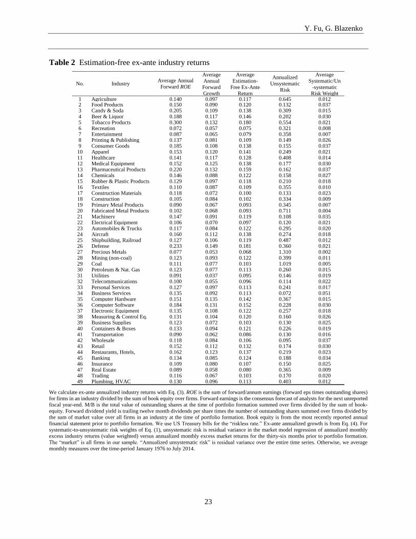
For the 49 industry portfolios, Table 2 presents average annual forward industry ROE, forward

industry growth, estimation-free ex-ante industry return, annualized unsystematic risk, and

systematic-to-unsystematic risk weights from Eq. (1) (with estimation-free industry ex-ante

returns and unsystematic risk estimated from the market model for thirty-six months prior to

portfolio formation at the end of calendar months) over all 49 industries. Other than unsystematic

risk, which is over the entire time series, we update each of these variates monthly and average

from January 1976 to July 2014.

Tobacco Products has the highest forward ROE (30.0% per annum) and Recreation has the

lowest (7.2% per annum). Defense has the greatest forward growth (14.9% per annum) and

Utilities has the smallest (3.7% per annum). Defense has the highest ex-ante return (18.1% per

annum) and Precious Metals has the lowest (6.8% per annum). Precious Metals has the highest

unsystematic risk (131%2 per annum) and Business Services has the lowest (7.2%2 per annum).

Wholesale has the largest systematic-to-unsystematic risk weight (3.7%) and Precious Metals has

the lowest (0.2%).

Y. Fu, G. Blazenko

10

4 Security selection

In our portfolio performance assessment, we study “non-equilibrium” portfolios. Investors follow

naïve 1/N’th investing, they make unrealistic presumptions that lead to ex-ante excess return

weight portfolios in Eq. (2), and/or they own less than the universe of N common shares in security

selection for either Eq. (1) or Eq. (2) portfolios. The monitoring costs Merton (1987) identifies

prevent active investors from owning all common shares and, thus, our security selection relates

to one of the earliest financial research questions: how many common shares diversify a portfolio?

Since both are important to investors, only the optimal trade-off between risk and return in

portfolios with well-behaved weights adequately answers the optimal diversification question.

Early evidence suggests that as few as ten common shares diversify a portfolio (Evans and

Archer, 1968; Lorie, 1975). Statman (1987) argues that diversification requires up to thirty

common shares. These authors plot average portfolio return standard-deviations against common-

share numbers in randomly constructed portfolios to identify when the plot “levels out” so that

there are no further diversification benefits. Elton and Gruber (1977) develop an analytic

expression for variance of portfolio return variance with respect to common-share numbers so that

investors can choose the volatility they accept from incomplete diversification. Bernstein (2000)

argues that the only way to correctly diversify a portfolio is to own the entire market. The superior

performance of 1/N’th investing in Jobson and Korkie (1981), Windcliff and Boyle (2004) and

DeMiguel, Garlappi, and Uppal (2009) also suggests extreme diversification. In our optimal

security selection, we weight high-return and high-risk common shares more highly than average

common shares, and thus we require more common shares than early evidence recommends but

markedly less than 1/N’th investing for diversification.

4.1 Methodology

We construct both systematic-to-unsystematic risk weight portfolios in Eq. (1) and ex-ante excess

return weight portfolios in Eq. (2) with both estimation-free and estimated ex-ante returns in Eq.

(3) and Eq. (6), respectively. Along with 1/N’th investing (that uses all available common shares

that meet our sample selection criteria at portfolio rebalancing), we compare five portfolios in

Sharpe ratio analysis. Since financial ratios have their vagaries when applied to individual common

shares, we limit the impact of extreme observations, by capping the weight of any common share

for portfolios of five or more common shares at twenty-five percent or less.

Y. Fu, G. Blazenko

11

4.2 The Realized Portfolio Out-Of-Sample Sharpe Ratio

Because weights in Eq. (1) maximize the ex-ante portfolio Sharpe ratio (see Appendix A),

consistency requires we measure portfolio performance with a realized Sharpe ratio. Portfolio

rebalancing is at the beginning of a calendar month (end of the prior calendar month) and we

measure the realized Sharpe ratio out-of-sample for the month following rebalancing. The one-

month realized Sharpe ratio (RSR) is the realized monthly portfolio return (with systematic-to-

unsystematic risk weights, ex-ante excess return weights, or 1/N’th weights as appropriate) less

the riskless interest rate for a one-month holding period divided by the portfolio return standard-

deviation (total rather than residual) for thirty-six months prior to portfolio rebalancing. Thus,

𝑅𝑆𝑅 = (�̃�𝑝,𝑡−𝑟𝑓,𝑡

�̃�𝑝,𝑡) (7)

Because of non-normality (confirmed with Kolmogorov-Smirnov tests), we use the temporal-

median as a central-tendency measure for RSR and, in addition, statistical tests are non-parametric,

𝑀𝑒𝑑𝑖𝑎𝑛 𝑅𝑆𝑅 =𝑚𝑒𝑑𝑖𝑎𝑛𝑡 = 1, 𝑇

(�̃�𝑝,𝑡−𝑟𝑓,𝑡

�̃�𝑝,𝑡) (8)

4.3 Security selection with estimation-free ex-ante returns

For estimation-free ex-ante returns in Eq. (3), forward earnings is the consensus forecast of

analysts for common share i for the next unreported fiscal year-end. M/B is share-price divided by

book equity. Dividend yield is trailing twelve month dividend per share divided by share-price (all

at portfolio rebalancing date t). Book equity is from the most recently reported quarterly or annual

financial statement prior to a portfolio rebalancing date t.

Fig. 2 plots temporal median realized monthly Sharpe ratios in Eq. (8) for the 1/N’th common

share strategy (that allocates a 1/N’th weight to each common share at the beginning of a month),

and portfolios with N*=1 to N*=200 highest ranked common-shares using two ranking methods:

first, by the ratio of estimation-free ex-ante excess return to unsystematic risk and, second, by

estimation-free ex-ante excess return (that is, Eq. (1) and Eq (2) portfolios). Weights for these

portfolios use the normalized value of each ranking variate. There are 200 portfolios for each

ranking variate. Unsystematic risk is from a market model regression for thirty-six months prior

Y. Fu, G. Blazenko

12

to portfolio formation. The “market” is the value-weighted portfolio of all common-shares in our

sample. We eliminate common shares from our sample at a month if they do not have at least 20

months for this regression. The “riskless rate” is from US Treasury bills.

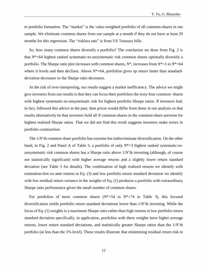
So, how many common shares diversify a portfolio? The conclusion we draw from Fig. 2 is

that N*=64 highest ranked systematic-to-unsystematic risk common shares optimally diversify a

portfolio. The Sharpe ratio plot increases with common shares, N*, increases from N*=1 to N*=64

where it levels and then declines. Above N*=64, portfolios gives up return faster than standard-

deviation decreases so the Sharpe ratio decreases.

At the risk of over-interpreting, our results suggest a market inefficiency. The advice we might

give investors from our results is that they can focus their portfolios the sixty-four common- shares

with highest systematic-to-unsystematic risk for highest portfolio Sharpe ratios. If investors had,

in fact, followed this advice in the past, then prices would differ from those in our analysis so that

results alternatively be that investors hold all N common-shares in the common-share universe for

highest realized Sharpe ratios. That we did not find this result suggests investors make errors in

portfolio construction.

The 1/N’th common share portfolio has extreme but indiscriminate diversification. On the other

hand, in Fig. 2 and Panel A of Table 3, a portfolio of only N*=3 highest ranked systematic-to-

unsystematic risk common shares has a Sharpe ratio above 1/N’th investing (although, of course

not statistically significant) with higher average returns and a slightly lower return standard

deviation (see Table 3 for details). The combination of high realized returns we identify with

estimation-free ex-ante returns in Eq. (3) and low portfolio return standard deviation we identify

with low residual return variance in the weights of Eq. (1) produces a portfolio with extraordinary

Sharpe ratio performance given the small number of common shares.

For portfolios of more common shares (N*=54 to N*=74 in Table 3), this focused

diversification yields portfolio return standard deviations lower than 1/N’th investing. While the

focus of Eq. (1) weights is a maximum Sharpe ratio rather than high returns or low portfolio return

standard deviation specifically, in application, portfolios with these weights have higher average

returns, lower return standard deviations, and statistically greater Sharpe ratios than the 1/N’th

portfolio (at less than the 1% level). These results illustrate that minimizing residual return risk in

Y. Fu, G. Blazenko

13

systematic-to-unsystematic risk portfolios in Eq. (1) is important for low portfolio return standard-

deviation and high Sharpe ratios.

In Panel B, because the focus of estimation-free ex-ante excess return weight portfolios is high

return with no risk consideration, they have the highest realized average returns in Table 3 but also

the highest return standard-deviations. Nonetheless, high returns dominate and ex-ante excess

return weight portfolios with N*=137 to N*=157 highest ranked ex-ante excess returns have

Sharpe ratios that statistically exceed the 1/N’th common share portfolio. Diversifying the high

risk of high return common shares returns requires a large number of common shares. A portfolio

with N*=147 ex-ante excess return selected common shares has the highest Sharpe ratio above

1/N’th investing. A portfolio with as few as N*=28 common shares has a Sharpe ratio about the

same as 1/N’th investing because of high realized returns we identify with estimation-free ex-ante

returns. This portfolio has the highest average realized monthly excess return and the highest return

standard deviation in Table 3 (also the highest return in either Table 3 or Table 4).

Fig. 2 Median Sharpe ratios for portfolios with estimation-free ex-ante returns

-0.01

0.04

0.09

0.14

0.19

0.24

0.29

0.34

0.39

1 51 101 151

Median

Sharpe

Ratio

Number of Common Shares in Portfolio, N*

1/N'th Common Share Strategy

Ranked by Estimation-Free Ex-Ante Excess Return

Ranked by Estimation-Free Ex-Ante Excess Return/Unsystematic Risk

Y. Fu, G. Blazenko

14

4.4 Security selection with estimated ex-ante returns

We estimate ex-ante returns with Eq. (6) at a monthly portfolio rebalancing date. Portfolio

rebalancing is at the beginning of a calendar month and we measure the realized Sharpe ratio for

the month following rebalancing. For systematic-to-unsystematic risk weights in Eq. (1),

unsystematic risk is from the regression in Eq. (5) that estimates factor betas for thirty-six months4

prior to portfolio formation at month t. We eliminate common shares from our sample at a month

if they do not have at least 20 months for this regression. The “riskless rate” is from US Treasury

bills.

Fig. 3 plots temporal median realized monthly Sharpe ratios in Eq. (8) for the 1/N’th common

share strategy (that allocates a 1/N’th weight to each common share at the beginning of a month),

and portfolios with N*=1 to N*=200 highest ranked common-shares using two ranking methods:

first, by the ratio of estimated ex-ante excess return to unsystematic risk and, second, by estimated

ex-ante excess return (that is, Eq. (1) and Eq. (2) portfolios). Weights for these portfolios use the

normalized value of each ranking variate. There are 200 portfolios for each ranking variate.

Details of highest Sharpe ratio portfolios in Fig. 3 are reported in Panel A of Table 4 for

portfolios with N*=46 to N*=66 common shares. These portfolios have higher average returns,

lower return standard-deviation, and statistically greater Sharpe ratios (at about the 10% level)

than the 1/N’th portfolio. The modest statistical significance of Sharpe ratio differences illustrates

the difficulty of outperforming the 1/N’th portfolio. The highest Sharpe ratio portfolio in Fig. 3

has N*=56 common shares.

In Panel B of Table 4, because the focus of ex-ante excess return weight portfolios is high return

with no risk consideration, they have the highest realized average returns in Table 4 but also the

highest return standard-deviations. However, there is no ex-ante excess return weight portfolio

with estimated ex-ante returns with a higher Sharpe ratio than the 1/N’th portfolio.

4 We use 36 months to be as temporally current as possible and to be consistent with realized Sharpe ratios in Eq. (7)

and Eq. (8). We get similar results when using a 60 month estimation window for ex-ante returns.

Y. Fu, G. Blazenko

15

Fig. 3 Median Sharpe ratios for portfolios formed with estimated ex-ante returns

4.5 Estimation-free versus estimated ex-ante returns

The answer to the question of the number of common shares to diversify a portfolio is almost

identical in Fig. 2 with estimation-free ex-ante returns and in Fig. 3 with estimated FF 5-factor ex-

ante returns. In Fig. 2, N*=64 highest ranked systematic-to-unsystematic risk common-shares

diversify a portfolio optimally, whereas, in Fig. 3, N*=56 highest ranked systematic-to-

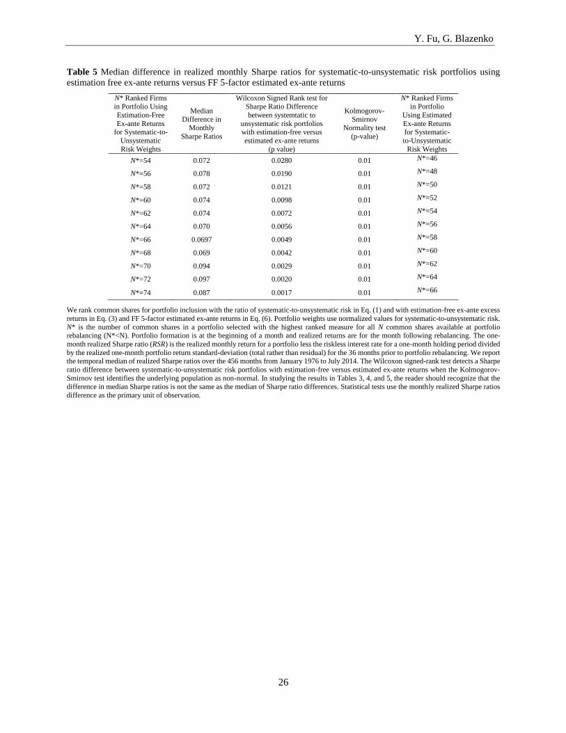
unsystematic risk common-shares optimally diversify a portfolio. Table 5 compares these

portfolios against one another. The Sharpe ratio of the estimation-free ex-ante return portfolio in

Fig. 2 with N*=64 common shares statistically exceeds that of the estimated ex-ante return

portfolio in Fig. 3 with N*=56 common shares (at a significance level less than one percent). Better

Sharpe ratio performance for systematic-to-unsystematic risk portfolios in Fig 2 with estimation-

free ex-ante returns compared to Fig 3 with estimated FF 5-factor ex-ante returns is primarily from

lower return standard deviation (see Table 3 versus Table 4).

A comparison of Panel B in Table 3 versus Panel B in Table 4 confirms that estimation-free ex-

ante returns identify higher realized returns than estimated ex-ante returns (in ex-ante excess return

weight portfolios). This difference is consistent with estimation-free ex-ante returns in Eq. (3)

being more timely and better able to capture temporal risk changes.

-0.01

0.04

0.09

0.14

0.19

0.24

0.29

0.34

0.39

1 51 101 151

Median

Sharpe

Ratio

Number of Common Shares in Portfolio, N*

1/N'th Industry Strategy

Ranked by FF 5Factor Estimated Ex-Ante Excess Return

Ranked by FF 5 Factor Ex-Ante Return / Unsystematic Risk

Y. Fu, G. Blazenko

16

An interesting question is why the lower return standard deviation in Panel A of Table 3 versus

Panel A of Table 4 (both for systematic-to-unsystematic risk weight portfolios)? Common shares

with high systematic-to-unsystematic risk weights in Eq. (1) minimize unsystematic risk but only

for a given ex-ante return. Thus, when we identify high returns with estimation-free ex-ante returns

(see Panel B of Table 3 compared to Panel B of Table 4), we are also better able to identify high

returns in combination with low unsystematic risk leading to lower portfolio return standard-

deviation. This is also the reason that systematic-to-unsystematic risk portfolios with both

estimation-free and FF 5-factor estimated ex-ante returns in Panel A of Table 3 and Panel A of

Table 4 have lower return standard deviation that the 1/N’th portfolio. Maximizing return relative

to risk is at the expense of some return. Average realized returns in Panel A are lower than in Panel

B in both Table 3 and Table 4. This “expense” is somewhat greater with estimation-free ex-ante

returns compared to estimated ex-ante returns with the result that both average returns and return

standard-deviations are lesser in Panel A of Table 3 compared to Panel A of Table 4.

6 Summary, conclusion, and suggestions for future research

In this paper, we jointly control portfolio weights and outperform 1/N’th investing in Sharpe ratio

analysis. We correct the weight misbehaviour of mean-variance analysis with systematic-to-

unsystematic risk weights that separate “good” priced risk in ex-ante returns from “bad” unpriced

risk in residual return variance. This separation obviates the need to estimate covariance directly.

Consistent with the theoretical work of Best and Grauer (1991), Chopra and Ziemba (1993), and

Ziemba (2003), we empirically find that mean returns are indeed paramount for portfolio

performance. In security selection, estimation-free ex-ante returns in systematic-to-unsystematic

risk weight portfolios have the highest Sharpe ratio.

Theoretical portfolio construction in Eq. (1) weights guides our analysis. But, we have been

crude in our application of this theory to assure readers that our results do not arise from data

“fishing.” Outperforming 1/N’th investing with well-behaved weights is the objective of our study.

Having achieved this objective, future research can attempt to better this performance with

alternative methods.

In general terms, the study of optimal portfolio weights should guide investor behaviour

(normative portfolio analysis). Unfortunately, weight misbehaviour in the existing mean-variance

literature impairs the ability of modern portfolio theory to offer this guidance. The well-behaved

Y. Fu, G. Blazenko

17

weights we propose have this ability. We find highest Sharpe ratios with sixty-four common shares

in security selection. These results challenge the advice of Bernstein (2000) and 1/N’th investing

to own the entire market for diversification. Beyond this result, we leave a detailed study of optimal

portfolio weights to future research, which we now merely anticipate.

An interesting investment question is whether there are performance “costs” to carbon or sin-

free “ethical” portfolios (carbon is oil & gas and coal and the sin industries are defense, adult

entertainment, tobacco, gambling, and alcohol). In the current paper, because we outperform the

1/N’th portfolio with sixty-four common shares, perhaps we will find that carbon is seldom a

component of high Sharpe ratio portfolios. Perhaps there are Sharpe ratio “costs” to investment

portfolios that are carbon or sin free. Perhaps sin common shares exceed their market weights.

We investigate equity allocation in a domestic context. An obvious extension is global equity

allocation. Our results suggest that global investing differs for investors in large and small

countries. We find domestically that sixty-four common shares in security selection maximize the

Sharpe ratio. Thus, despite theoretical equilibrium analysis to the contrary, for individually optimal

portfolios, investors need not own all common shares in security selection. Internationally, large

countries have a large number of common shares. Large numbers make investors more likely to

find high systematic-to-unsystematic risk common shares domestically and they can, thus, avoid

the exchange rate risk of global investing. Opposite results are true for investors in small countries.

We investigate a particular mean-variance investor who maximizes the Sharpe ratio. We can

undertake a similar analysis for an investor with general mean-variance utility. A principal

question is whether a low risk-averse investor favours ex-ante excess return weight portfolios and

a high risk-averse investor favours systematic-to-unsystematic risk portfolios. If different risk-

averse investors choose different portfolios, then we uncover a violation of the hypothesis of two-

fund separation.

To maximize Sharpe ratios, our results suggest that investors need not own all common shares

in security selection. However, we investigate only portfolios with long-positions. Alternatively,

common shares with least portfolio appeal measured by Eq. (1) may be candidates for short-

positions in non-equilibrium long-short portfolios for enhanced Sharpe ratios. Transactions costs

for short-positions may exceed those of long-positions.

Of course, any conjecture we make above requires confirmation in future research.

Y. Fu, G. Blazenko

18

6 Appendix A

In this appendix, with equilibrium returns from a linear return model, we derive the portfolio

weights in Eq. (1) that maximize the Sharpe ratio. Realized return, �̃�𝑖, for asset i depends on the

return on a benchmark portfolio, �̃�𝐺 , and a zero-mean perturbation that is independent over time,

independent over assets, and independent of the return on the benchmark portfolio,

�̃�𝑖 = 𝛼𝑖 + 𝛽𝑖 ∙ �̃�𝐺 + 𝜀�̃� i=1,2,…,N (A1)

The variance of the perturbation, 𝜎𝜀𝑖

2 , is unsystematic risk.

A single factor in Eq. (A1) is without loss of generality. Alternatively, if multiple factors

determine returns, we show in appendix B that an asset’s excess return is, nonetheless, a beta times

the excess return of a benchmark portfolio. Bali and Cakici (2010) find no difference in global

asset-pricing tests with single versus multiple factors. In domestic asset-pricing tests, Fama and

French (1992) find multiple return factors but a beta estimate over a multi-year estimation window

does not capture temporal risk changes. Thus, within the confines of estimation error,

supplementary factors figure prominently in testing because they are more current than a beta

estimate and act as updates for the unobserved true beta. For example, the likelihood that a high-

risk asset has high average past and future returns is greater than for a low risk asset and, thus, a

“momentum” factor (high average returns in the recent past) helps explain realized returns beyond

a dated single-factor beta estimate.

Let 𝐸(�̃�𝑖) and 𝜎𝑖2 be ex-ante return and return variance for asset i. Similar measures for a

portfolio are 𝐸(�̃�𝑝) and 𝜎𝑝2. The investor’s portfolio problem is,

𝑚𝑎𝑥

𝑥1, 𝑥2, … , 𝑥𝑁[

𝐸(�̃�𝑝)−𝑟𝑓

𝜎𝑝] subject to

1

1N

k

k

x

(A2)

where 𝑟𝑓 is the riskless rate and 𝑥𝑖 is the portfolio weight for asset i from among N risky assets.

Since the Sharpe ratio in Eq. (A2) is homogeneous of degree zero, we can ignore the constraint if

we subsequently normalize weights to sum to unity.

With returns from (A1), the portfolio Sharpe ratio is,

Y. Fu, G. Blazenko

19

∑ 𝑥𝑘(𝐸(�̃�𝑘)−𝑟𝑓)𝑁

𝑘=1

[(∑ 𝑥𝑘𝛽𝑘𝑁𝑘=1 )

2𝜎𝐺

2+∑ 𝑥𝑘2𝑁

𝑘=1 𝜎𝜀𝑘2 ]

1/2 (A3)

where 𝜎𝐺2 is the variance of the rate of return for the common factor. First order conditions are,

[𝐸(�̃�𝑖) − 𝑟𝑓]𝜎𝑝2 − [(∑ 𝑥𝑘𝛽𝑘

𝑁𝑘=1 )𝜎𝐺

2𝛽𝑖 + 𝑥𝑖𝜎𝜀𝑖

2 ] ∙ [∑ 𝑥𝑘(𝐸(�̃�𝑘) − 𝑟𝑓)𝑁𝑘=1 ]=0, i=1,2,…,N (A4)

which are the Elton, Gruber, Padberg (1976) equations that implicitly specify optimal portfolio

weights when a linear return model generates returns.

Define,

𝑧𝑖 = [∑ 𝑥𝑘(𝐸(�̃�𝑘)−𝑟𝑓)𝑁

𝑘=1

𝜎𝑝2 ] 𝑥𝑖, i=1,2,…,N (A5)

Substitute (A5) into Eq. (A4) and solve for 𝑧𝑖,

𝑧𝑖 =𝐸(�̃�𝑖)−𝑟𝑓

𝜎𝜀𝑖2 − [∑ 𝑧𝑘𝛽𝑘

𝑁𝑘=1 ] [

𝛽𝑖𝜎𝐺2

𝜎𝜀𝑖2 ] (A6)

Multiply Eq. (A6) by 𝛽𝑖, sum, and solve for ∑ 𝑧𝑘𝛽𝑘𝑁𝑘=1 ,

∑ 𝑧𝑘𝛽𝑘𝑁𝑘=1 =

∑ [𝐸(�̃�𝑘)−𝑟𝑓]𝛽𝑘/𝜎𝜀𝑘2𝑁

𝑘=1

1+∑ 𝛽𝑘2𝜎𝐺

2/𝜎𝜀𝑘2𝑁

𝑘=1

(A7)

Define 𝐴 = (∑ 𝛽𝑘2/𝜎𝜀𝑘

2𝑁𝑘=1 )𝜎𝐺

2 (A8)

Substitute Eqs. (A7) and (A8) into Eq. (A6),

𝑧𝑖 =𝐸(�̃�𝑖)−𝑟𝑓

𝜎𝜀𝑖2 − [

∑ [𝐸(�̃�𝑘)−𝑟𝑓]𝛽𝑘/𝜎𝜀𝑘2𝑁

𝑘=1

1+𝐴] [

𝛽𝑖𝜎𝐺2

𝜎𝜀𝑖2 ] (A9)

Since the excess return of asset i is 𝛽𝑖 times that of portfolio G,

𝐸(�̃�𝑖) − 𝑟𝑓 = 𝛽𝑖[𝐸(�̃�𝐺) − 𝑟𝑓] i=1,2,…,N (A10)

where GE R is the expected return on the benchmark portfolio. Substitute Eq. (A10) into (A9),

𝑧𝑖 =𝛽𝑖[𝐸(�̃�𝐺)−𝑟𝑓]

𝜎𝜀𝑖2 (1+𝐴)

(A11)

Y. Fu, G. Blazenko

20

Because the numerator of (A11) is the risk premium for security i from Eq. (A10),

𝑧𝑖 =𝐸(�̃�𝑖)−𝑟𝑓

𝜎𝜀𝑖2 (1+𝐴)

(A12)

Normalize to eliminate the constant of proportionality to produce the weights in Eq. (1).

7 Appendix B

In this appendix, we show that if multiple factors determine returns, then, nonetheless, excess

return for an asset is the asset-beta multiplied by excess return of a benchmark portfolio.

Consider two portfolios, 1 and 2. Two factors (A and B) determine returns (the extension to

more than two factors is transparent). First,

�̃�2 = 𝐸(�̃�2) + 𝑔𝐴 ∙ 𝑓𝐴 + 𝑔𝐵 ∙ 𝑓𝐵 + 𝜉+ (B1)

where, 𝑓𝐴 = �̃�𝐴 − 𝐸(�̃�𝐴) and 𝑓𝐵 = �̃�𝐵 − 𝐸(�̃�𝐵) are the unexpected parts of factor A and B,

respectively. The excess return of portfolio 2 is

𝐸(�̃�2) − 𝑟𝑓 = 𝑔𝐴 ∙ [𝐸(�̃�𝐴) − 𝑟𝑓] + 𝑔𝐵 ∙ [𝐸(�̃�𝐵) − 𝑟𝑓] (B2)

The return of portfolio 2 determines the return of portfolio 1 plus an error,

�̃�1 = 𝛼 + 𝛽 ∙ �̃�2 + 𝜀̃ (B3)

Substitute (B1) into (B3) and,

�̃�1 = 𝛼 + 𝛽 ∙ [𝐸(�̃�2) + 𝑔𝐴 ∙ 𝑓𝐴 + 𝑔𝐵 ∙ 𝑓𝐵 + 𝜉] + 𝜀̃

= 𝛼 + 𝛽 ∙ 𝐸(�̃�2) + 𝛽 ∙ 𝑔𝐴 ∙ 𝑓𝐴 + 𝛽 ∙ 𝑔𝐵 ∙ 𝑓𝐵 + 𝛽 ∙ 𝜉 + 𝜀̃

= [𝛼 + 𝛽 ∙ 𝐸(�̃�2)] + (𝛽 ∙ 𝑔𝐴) ∙ 𝑓𝐴 + (𝛽 ∙ 𝑔𝐵) ∙ 𝑓𝐵 + [𝛽 ∙ 𝜉 + 𝜀̃] (B4)

Take the expectation of (B3),

𝐸(�̃�1) = 𝛼 + 𝛽 ∙ 𝐸(�̃�2) (B5)

Replace the first term of (B4) with (B5),

�̃�1 = 𝐸(�̃�1) + (𝛽𝑔𝐴) ∙ 𝑓𝐴 + (𝛽𝑔𝐵) ∙ 𝑓𝐵 + [𝛽 ∙ 𝜉 + 𝜀̃] (B6)

Eq. (B6) shows that, like portfolio 2, factors A and B determine the return of portfolio 1 but with

factor sensitivities Ag and Bg . The excess return of portfolio 1 is,

Y. Fu, G. Blazenko

21

𝐸(�̃�1) − 𝑟𝑓 = (𝛽𝑔𝐴) ∙ [𝐸(�̃�𝐴) − 𝑟𝑓] + (𝛽𝑔𝐵) ∙ [𝐸(�̃�𝐵) − 𝑟𝑓]

=𝛽 ∙ {𝑔𝐴 ∙ [𝐸(�̃�𝐴) − 𝑟𝑓] + 𝑔𝐵 ∙ [𝐸(�̃�𝐵) − 𝑟𝑓]} = 𝛽 ∙ [𝐸(�̃�2) − 𝑟𝑓]

Thus, the excess return of portfolio 1 is 𝛽 times that of portfolio 2.

Y. Fu, G. Blazenko

22

Table 1 Realized industry portfolio returns

No. Industry

Annualized

Average Monthly

Realized Return

Estimated

Beta

Average Monthly

Return Standard-

Deviation

Average Weight

in Market

Portfolio

Average #

of Firms in

Portfolio

1 Agriculture 0.151 0.952 0.079 0.001 6 2 Food Products 0.145 0.582 0.024 0.022 47 3 Candy & Soda 0.150 0.709 0.044 0.011 7 4 Beer & Liquor 0.146 0.616 0.033 0.011 9 5 Tobacco Products 0.209 0.572 0.060 0.010 4 6 Recreation 0.134 1.097 0.053 0.004 19 7 Entertainment 0.177 1.479 0.098 0.007 35 8 Printing & Publishing 0.119 1.013 0.041 0.007 22 9 Consumer Goods 0.109 0.687 0.029 0.024 50

10 Apparel 0.168 1.200 0.062 0.005 36 11 Healthcare 0.156 1.016 0.078 0.004 40 12 Medical Equipment 0.137 0.976 0.041 0.011 75 13 Pharmaceutical Products 0.140 0.773 0.031 0.075 121 14 Chemicals 0.130 1.086 0.046 0.030 59 15 Rubber & Plastic Products 0.121 1.018 0.054 0.002 20 16 Textiles 0.144 1.258 0.078 0.002 20 17 Construction Materials 0.125 1.178 0.047 0.011 55 18 Construction 0.124 1.479 0.076 0.003 34 19 Primary Metal Products 0.117 1.428 0.083 0.012 48 20 Fabricated Metal Products 0.044 1.354 0.113 0.000 7 21 Machinery 0.139 1.226 0.048 0.039 100 22 Electrical Equipment 0.127 1.122 0.047 0.008 37 23 Automobiles & Trucks 0.123 1.179 0.063 0.022 46 24 Aircraft 0.166 1.091 0.054 0.012 15 25 Shipbuilding, Railroad

Eq.

0.197 1.182 0.096 0.001 6 26 Defense 0.169 0.811 0.062 0.002 6 27 Precious Metals 0.121 0.720 0.134 0.005 16 28 Mining (non-coal) 0.144 1.262 0.068 0.003 11 29 Coal 0.137 1.152 0.116 0.001 6 30 Petroleum & Nat. Gas 0.143 0.830 0.040 0.105 118 31 Utilities 0.129 0.483 0.022 0.056 130 32 Telecommunications 0.121 0.794 0.031 0.067 72 33 Personal Services 0.131 1.046 0.054 0.004 29 34 Business Services 0.119 1.138 0.040 0.017 126 35 Computer Hardware 0.143 1.383 0.093 0.031 71 36 Computer Software 0.118 1.137 0.058 0.060 188 37 Electronic Equipment 0.137 1.446 0.081 0.040 162 38 Measuring & Control Eq. 0.139 1.274 0.059 0.009 59 39 Business Supplies 0.113 0.947 0.039 0.020 44 40 Containers & Boxes 0.140 0.969 0.039 0.002 10 41 Transportation 0.143 1.087 0.042 0.020 80 42 Wholesale 0.122 0.993 0.033 0.011 85 43 Retail 0.139 0.989 0.042 0.055 152 44 Restaurants, Hotels,

Motels

0.136 0.910 0.045 0.008 45 45 Banking 0.135 1.083 0.048 0.080 284 46 Insurance 0.141 1.021 0.038 0.044 110 47 Real Estate 0.164 1.153 0.076 0.001 13 48 Trading 0.155 1.438 0.063 0.021 104 49 Plumbing, HVAC 0.151 1.029 0.073 0.005 18

Annualized return is twelve-times the value weighted average monthly return for firms in an industry from January 1976 to July 2014. The beta uses the value-weighted return of all firms in our sample as the “market” portfolio. Monthly return standard-deviation is for the value weighted

average return for firms in an industry from January 1976 to July 2014. Industry value weights are for all firms in an industry in our sample

measured monthly and averaged over the entire time-period.

Y. Fu, G. Blazenko

23

Table 2 Estimation-free ex-ante industry returns

No. Industry Average Annual

Forward ROE

Average

Annual

Forward Growth

Average

Estimation-

Free Ex-Ante Return

Annualized

Unsystematic

Risk

Average

Systematic/Un

-systematic Risk Weight

1 Agriculture 0.140 0.097 0.117 0.645 0.012 2 Food Products 0.150 0.090 0.120 0.132 0.037 3 Candy & Soda 0.205 0.109 0.138 0.309 0.015 4 Beer & Liquor 0.188 0.117 0.146 0.202 0.030 5 Tobacco Products 0.300 0.132 0.180 0.554 0.021 6 Recreation 0.072 0.057 0.075 0.321 0.008 7 Entertainment 0.087 0.065 0.079 0.358 0.007 8 Printing & Publishing 0.137 0.081 0.109 0.149 0.026 9 Consumer Goods 0.185 0.108 0.138 0.155 0.037

10 Apparel 0.153 0.120 0.141 0.249 0.021 11 Healthcare 0.141 0.117 0.128 0.408 0.014 12 Medical Equipment 0.152 0.125 0.138 0.177 0.030 13 Pharmaceutical Products 0.220 0.132 0.159 0.162 0.037 14 Chemicals 0.146 0.088 0.122 0.158 0.027 15 Rubber & Plastic Products 0.129 0.097 0.118 0.210 0.018 16 Textiles 0.110 0.087 0.109 0.355 0.010 17 Construction Materials 0.118 0.072 0.100 0.133 0.023 18 Construction 0.105 0.084 0.102 0.334 0.009 19 Primary Metal Products 0.090 0.067 0.093 0.345 0.007 20 Fabricated Metal Products 0.102 0.068 0.093 0.711 0.004 21 Machinery 0.147 0.091 0.119 0.108 0.035 22 Electrical Equipment 0.106 0.070 0.097 0.120 0.021 23 Automobiles & Trucks 0.117 0.084 0.122 0.295 0.020 24 Aircraft 0.160 0.112 0.138 0.274 0.018 25 Shipbuilding, Railroad

Eq.

0.127 0.106 0.119 0.487 0.012 26 Defense 0.233 0.149 0.181 0.360 0.021 27 Precious Metals 0.077 0.053 0.068 1.310 0.002 28 Mining (non-coal) 0.123 0.093 0.122 0.399 0.011 29 Coal 0.111 0.077 0.103 1.019 0.005 30 Petroleum & Nat. Gas 0.123 0.077 0.113 0.260 0.015 31 Utilities 0.091 0.037 0.095 0.146 0.019 32 Telecommunications 0.100 0.055 0.096 0.114 0.022 33 Personal Services 0.127 0.097 0.113 0.241 0.017 34 Business Services 0.135 0.092 0.113 0.072 0.051 35 Computer Hardware 0.151 0.135 0.142 0.367 0.015 36 Computer Software 0.184 0.131 0.152 0.228 0.030 37 Electronic Equipment 0.135 0.108 0.122 0.257 0.018 38 Measuring & Control Eq. 0.131 0.104 0.120 0.160 0.026 39 Business Supplies 0.123 0.072 0.103 0.130 0.025 40 Containers & Boxes 0.133 0.094 0.121 0.226 0.019 41 Transportation 0.090 0.062 0.086 0.130 0.016 42 Wholesale 0.118 0.084 0.106 0.095 0.037 43 Retail 0.152 0.112 0.132 0.174 0.030 44 Restaurants, Hotels,

Motels

0.162 0.123 0.137 0.219 0.023 45 Banking 0.134 0.085 0.124 0.188 0.034 46 Insurance 0.109 0.080 0.107 0.150 0.025 47 Real Estate 0.089 0.058 0.080 0.365 0.009 48 Trading 0.116 0.067 0.103 0.170 0.020 49 Plumbing, HVAC 0.130 0.096 0.113 0.403 0.012

We calculate ex-ante annualized industry returns with Eq. (3). ROE is the sum of forward/annum earnings (forward eps times outstanding shares) for firms in an industry divided by the sum of book equity over firms. Forward earnings is the consensus forecast of analysts for the next unreported

fiscal year-end. M/B is the total value of outstanding shares at the time of portfolio formation summed over firms divided by the sum of book-

equity. Forward dividend yield is trailing twelve month dividends per share times the number of outstanding shares summed over firms divided by the sum of market value over all firms in an industry at the time of portfolio formation. Book equity is from the most recently reported annual

financial statement prior to portfolio formation. We use US Treasury bills for the “riskless rate.” Ex-ante annualized growth is from Eq. (4). For

systematic-to-unsystematic risk weights of Eq. (1), unsystematic risk is residual variance in the market model regression of annualized monthly excess industry returns (value weighted) versus annualized monthly excess market returns for the thirty-six months prior to portfolio formation.

The “market” is all firms in our sample. “Annualized unsystematic risk” is residual variance over the entire time series. Otherwise, we average

monthly measures over the time-period January 1976 to July 2014.

Y. Fu, G. Blazenko

24

Table 3 Realized Sharpe ratios for portfolios formed by ranking individual common shares by

systematic-to-unsystematic risk (Panel A) and by ex-ante excess return (Panel B) using, in each

case, estimation-free ex-ante returns

N* Ranked

Firms in Portfolio

Median

Realized Sharpe Ratio

Average Monthly

Excess-return

Average Monthly

Return Standard Deviation

Median Sharpe Ratio Difference

with 1/N’th

portfolio

Wilcoxon Signed

Rank test for Sharpe ratio

difference between

N* and 1/N’th portfolio (p value)

Kolmogorov-Smirnov

Normality test

(p value)

Panel A: Portfolios Ranked by Estimation Free Ex-ante Excess Return/Unsystematic Risk

N*=3 0.238 0.00952 0.0539 -0.026 0.5727 0.06

N*=54 0.348 0.00954 0.0384 0.098 0.0000 0.01

N*=56 0.366 0.00956 0.0383 0.108 0.0000 0.01

N*=58 0.377 0.00968 0.0383 0.122 0.0000 0.01

N*=60 0.375 0.00981 0.0383 0.114 0.0000 0.01

N*=62 0.398 0.00993 0.0382 0.109 0.0000 0.01

N*=64 0.401 0.00982 0.0382 0.113 0.0000 0.01

N*=66 0.393 0.00982 0.0381 0.114 0.0000 0.01

N*=68 0.379 0.00989 0.0381 0.125 0.0000 0.01

N*=70 0.380 0.00992 0.0381 0.128 0.0000 0.01

N*=72 0.377 0.00998 0.0381 0.131 0.0000 0.01

N*=74 0.388 0.00989 0.0381 0.123 0.0000 0.01

Panel B: Portfolios Ranked by Estimation Free Ex-ante Excess Return

N*=28 0.214 0.01534 0.0765 0.045 0.0298 0.01

N*=137 0.261 0.01334 0.0676 0.052 0.0004 0.01

N*=139 0.263 0.01355 0.0675 0.053 0.0002 0.01

N*=141 0.263 0.01327 0.0675 0.052 0.0002 0.01

N*=143 0.265 0.01344 0.0675 0.054 0.0001 0.01

N*=145 0.269 0.01350 0.0674 0.051 0.0001 0.01

N*=147 0.272 0.01354 0.0674 0.051 0.0001 0.01

N*=149 0.261 0.01345 0.0674 0.051 0.0001 0.01

N*=151 0.266 0.01344 0.0673 0.046 0.0001 0.01

N*=153 0.265 0.01329 0.0673 0.047 0.0001 0.01

N*=155 0.263 0.01341 0.0672 0.043 0.0002 0.01

N*=157 0.263 0.01319 0.0672 0.043 0.0002 0.01

1/N’th

Common Share Portfolio

0.235 0.0083 0.0563

We rank common shares for portfolio inclusion in two ways: with the ratio of systematic-to-unsystematic risk in Eq. (1) and with ex-ante excess

returns in Eq. (2). In both cases, ex-ante return is from equation (3). Portfolio weights use normalized values for these two measures, respectively.

N* is the number of common shares in a portfolio selected with the highest ranked measure for all N common shares available at portfolio rebalancing (N*<N). The 1/N’th common share strategy has a 1/N weight in each common share. Portfolio formation is at the beginning of a month

and realized returns are for the month following rebalancing. The one-month realized Sharpe ratio (RSR) is the realized monthly return for a portfolio

less the riskless interest rate for a one-month holding period divided by the realized one-month portfolio return standard-deviation (total rather than residual) for the 36 months prior to portfolio rebalancing. We report the temporal median of realized Sharpe ratios over the 456 months from

January 1976 to July 2014. The Wilcoxon signed-rank test detects a Sharpe ratio difference between N* portfolios and 1/N’th common share

investing when the Kolmogorov-Smirnov test identifies the underlying population as non-normal. In comparing results in Tables 3, 4, and 5, the reader should recognize that the difference in median Sharpe ratios is not the same as the median Sharpe ratio difference. Statistical tests use the

monthly realized Sharpe ratios difference as the primary unit of observation.

Y. Fu, G. Blazenko

25

Table 4 Realized Sharpe ratios for portfolios formed by ranking individual common shares by

systematic-to-unsystematic risk (Panel A) and ex-ante excess return (Panel B) using, in each

case, estimated FF 5-Factor ex-ante returns

N* Ranked

Firms in Portfolio

Median

Realized Sharpe Ratio

Average Monthly

Excess-return

Average Monthly

Return Standard Deviation

Median Sharpe Ratio Difference

with 1/N’th

portfolio

Wilcoxon Signed

Rank test for Sharpe ratio

difference between

N* and 1/N’th portfolio (p value)

Kolmogorov-Smirnov

Normality test

(p value)

Panel A: Portfolios Ranked by Estimation Free Ex-ante Excess Return/Unsystematic Risk

N*=3 0.157 0.00782 0.0567 0.034 0.8728 0.01

N*=46 0.285 0.01069 0.0518 0.022 0.0558 0.01

N*=48 0.280 0.01061 0.0518 0.021 0.0599 0.01

N*=50 0.266 0.01053 0.0518 0.006 0.0797 0.01

N*=52 0.264 0.01051 0.0519 0.015 0.0793 0.01

N*=54 0.274 0.01038 0.0519 0.018 0.0781 0.01

N*=56 0.294 0.01036 0.0519 0.021 0.0800 0.01

N*=58 0.289 0.01036 0.0519 0.022 0.0769 0.01

N*=60 0.280 0.01038 0.0519 0.017 0.0780 0.01

N*=62 0.277 0.01029 0.0519 0.010 0.0878 0.01

N*=64 0.270 0.01027 0.0519 0.011 0.1045 0.01

N*=66 0.270 0.01023 0.0519 0.011 0.1091 0.01

Panel B: Portfolios Ranked by Estimation Free Ex-ante Excess Return

N*=28 0.082 0.01132 0.1570 -0.083 0.0034 0.01

N*=137 0.123 0.01135 0.1126 -0.067 0.0011 0.01

N*=139 0.121 0.01118 0.1121 -0.068 0.0009 0.01

N*=141 0.120 0.01118 0.1119 -0.076 0.0010 0.01

N*=143 0.128 0.01116 0.1116 -0.074 0.0009 0.01

N*=145 0.125 0.01111 0.1113 -0.063 0.0009 0.01

N*=147 0.131 0.01116 0.1111 -0.062 0.0010 0.01

N*=149 0.124 0.01115 0.1108 -0.063 0.0010 0.01

N*=151 0.124 0.01113 0.1105 -0.064 0.0010 0.01

N*=153 0.123 0.01112 0.1103 -0.061 0.0011 0.01

N*=155 0.122 0.01114 0.1100 -0.062 0.0012 0.01

N*=157 0.123 0.01115 0.1097 -0.064 0.0011 0.01

1/N’th

Common Share

Portfolio

0.235 0.0083 0.0563

We rank common shares for portfolio inclusion in two ways: with the ratio of systematic-to-unsystematic risk in Eq. (1) and with ex-ante excess

returns in Eq. (2). In both cases, we estimate ex-ante return with the FF 5-factor model. Portfolio weights use normalized values for these two

measures, respectively. N* is the number of common shares in a portfolio selected with the highest ranked measure for all N common shares available at portfolio rebalancing (N*<N). The 1/N’th common share strategy has a 1/N weight in each common share. Portfolio formation is at the

beginning of a month and realized returns are for the following month. The one-month realized Sharpe ratio (RSR) is the realized monthly return

for a portfolio less the riskless interest rate for a one-month holding period divided by the realized one-month portfolio return standard-deviation (total rather than residual) for the 36 months prior to portfolio rebalancing. We report the temporal median of realized Sharpe ratios over the 456

months from January 1976 to July 2014. The Wilcoxon signed-rank test detects a Sharpe ratio difference between N* portfolios and 1/N’th common

share investing when the Kolmogorov-Smirnov test identifies the underlying population as non-normal. In comparing results in Tables 3, 4, and 5, the reader should recognize that the difference in median Sharpe ratios is not the same as the median of Sharpe ratio differences. Statistical tests

use the monthly realized Sharpe ratios difference as the primary unit of observation.

Y. Fu, G. Blazenko

26

Table 5 Median difference in realized monthly Sharpe ratios for systematic-to-unsystematic risk portfolios using

estimation free ex-ante returns versus FF 5-factor estimated ex-ante returns

N* Ranked Firms in Portfolio Using

Estimation-Free

Ex-ante Returns for Systematic-to-

Unsystematic

Risk Weights

Median Difference in

Monthly

Sharpe Ratios

Wilcoxon Signed Rank test for Sharpe Ratio Difference

between systemtatic to

unsystematic risk portfolios with estimation-free versus

estimated ex-ante returns

(p value)

Kolmogorov-Smirnov

Normality test

(p-value)

N* Ranked Firms in Portfolio

Using Estimated

Ex-ante Returns for Systematic-

to-Unsystematic

Risk Weights

N*=54 0.072 0.0280 0.01 N*=46

N*=56 0.078 0.0190 0.01 N*=48

N*=58 0.072 0.0121 0.01 N*=50

N*=60 0.074 0.0098 0.01 N*=52

N*=62 0.074 0.0072 0.01 N*=54

N*=64 0.070 0.0056 0.01 N*=56

N*=66 0.0697 0.0049 0.01 N*=58

N*=68 0.069 0.0042 0.01 N*=60

N*=70 0.094 0.0029 0.01 N*=62

N*=72 0.097 0.0020 0.01 N*=64

N*=74 0.087 0.0017 0.01 N*=66

We rank common shares for portfolio inclusion with the ratio of systematic-to-unsystematic risk in Eq. (1) and with estimation-free ex-ante excess

returns in Eq. (3) and FF 5-factor estimated ex-ante returns in Eq. (6). Portfolio weights use normalized values for systematic-to-unsystematic risk.

N* is the number of common shares in a portfolio selected with the highest ranked measure for all N common shares available at portfolio rebalancing (N*<N). Portfolio formation is at the beginning of a month and realized returns are for the month following rebalancing. The one-

month realized Sharpe ratio (RSR) is the realized monthly return for a portfolio less the riskless interest rate for a one-month holding period divided

by the realized one-month portfolio return standard-deviation (total rather than residual) for the 36 months prior to portfolio rebalancing. We report the temporal median of realized Sharpe ratios over the 456 months from January 1976 to July 2014. The Wilcoxon signed-rank test detects a Sharpe

ratio difference between systematic-to-unsystematic risk portfolios with estimation-free versus estimated ex-ante returns when the Kolmogorov-

Smirnov test identifies the underlying population as non-normal. In studying the results in Tables 3, 4, and 5, the reader should recognize that the difference in median Sharpe ratios is not the same as the median of Sharpe ratio differences. Statistical tests use the monthly realized Sharpe ratios

difference as the primary unit of observation.

Y. Fu, G. Blazenko

27

References

Ang, A., Hodrick, R., Xing, Y., and Zhang, X. (2006) “The Cross-Section of Volatility and

Expected Returns,” Journal of Finance 61(1), 259-299.

Bali, T.G., Cakici, N.: World market risk, industry-specific risk, and expected returns in

international stock markets. J. Bank. Financ. 34(8), 1152-65 (2010)

Bartunek, R.S., Chowdhury, M. (1995) “Implied Volatility vs. Garch: A Comparison of

Forecasts,” Managerial Finance 21(10), 59-73.

Bernstein, W.J.: The 15-stock diversification myth.

http://www.efficientfrontier.com/ef/900/15st.htm (2000). Accessed August 7, 2015.

Best, M.J., Grauer, R.R.: Sensitivity of mean/variance efficient portfolios to changes in asset

means: some analytical and computational results. Rev. Financ. Stud. 4(2), 315-342 (1991)

Best, M.J., Grauer, R.: Positively weighted minimum-variance efficient portfolios and the structure

of expected asset returns. J. Financ. Quant. Anal. 27(4), 513-537 (1992)

Black, F., Litterman, R.: Industry portfolio optimization. Financ. Anal. J. 48(7), 28-43 (1992)

Blazenko, G.W., Fu, Y.: Value versus growth in dynamic equity investing. Manage. Financ. 39(3),

272-305 (2013)

Blazenko, G.W., Pavlov, A.D.: Investment timing for dynamic business expansion. Financ.

Manage. 38(4), 837-860 (2009)

Chopra, V., Ziemba, W.T.: Errors in means, variances, and covariances in optimal portfolio choice.

J. Portfolio Manage. 19(2), 6-11 (1993)

Chung, D.Y., Dusan, I., Perignon, C.: Repurchasing shares on a second trading line. Rev. Financ.

11(2), 253-285 (2007)

DeMiguel, V., Garlappi, L., Uppal, R.: Optimal versus naïve diversification: how inefficient is the

1/N portfolio strategy? Rev. Financ. Stud. 22(7), 1915-1953 (2009)

Dickinson, J. P. 1974. The reliability of estimation procedures in portfolio analysis. J. Financial

Quant. Anal. 9 447–462.

Elton, E.J., Gruber, M.J.: Risk reduction and portfolio size: an analytic solution. J. Bus. 50(4), 415-

437 (1977)

Elton, E.J., Gruber, M. J., Padberg, M.W.: Simple criteria for optimal portfolio selection. J. Financ.

31(7), 1341-1357 (1976)

Evans J., Archer S.: Diversification and the reduction of dispersion: an empirical analysis, J.

Financ. 23(7), 761-67 (1968)

Fama, E.F., French, K.R.: The cross-section of expected stock returns. J. Financ. 47(2), 427-465

(1992)

Fama, E.F., French, K.R.: Industry cost of capital. J. Financ. Econ. 43(2), 153-193 (1997)

Fama, E., French, K.R.: A five-factor asset pricing model. J. Financ. Econ. (forthcoming, 2015)

Fu, Y., Blazenko, G.W.: Returns for dividend paying and non-dividend paying firms. Int. J. Bus.

Financ. Res. 9(2), 1-15 (2015)

Y. Fu, G. Blazenko

28

Grullon, G., Michaely, R.: Dividends, share repurchases and the substitution hypothesis. J. Financ.

57(4), 1649-1684 (2002)

Grullon, G., Paye, B., Underwood, S., Weston, J.P.: Has the propensity to pay out declined? J.

Financ. Quant. Anal. 46(1), 1-24 (2011)

Golosnoy, V., Okhrin, Y.: Flexible shrinkage in portfolio selection. J. Econ. Dyn. Control 33(2),

317-328 (2009)

Hou, K., Xue, C., Zhang, L.: Digesting anomalies: an investment approach. Rev. Financ. Stud.

(forthcoming 2015).

Jarrow, R. and Rudd, A. “A Comparison of the APT and CAPM” Journal of Banking & Finance,

1983, Vol. 7(2), 295-303.

Jobson, J. D., B. Korkie. 1981. Putting Markowitz theory to work. J. Portfolio Management 7 70–

74.

Kan, R., Smith, D.R.: The Distribution of the sample minimum-variance frontier. Manage. Sc.

54(5), 1364-80 (2008)

Lee, B-S., Rui, O.M.: Time series behavior of share repurchases and dividends. J. Financ. Quant.

Anal. 42(1), 119-142 (2007)

Lintner, John. 1965. “The Valuation of Risk Assets and the Selection of Risky Investments in Stock

Portfolios and Capital Budgets.” Review of Economics and Statistics, vol. 47, no. 1 (February):13-37.

Lorie J.: Diversification: Old and new. J. Portfolio Manage. 1(2), 25-28 (1975)

Lowry, R. (2012). Concepts & applications of inferential statistics. (2012).

http://vassarstats.net/textbook/ch12a.html, Accessed August 7, 2015.

Markowitz, H.M.: Portfolio selection. J. Financ. 7(1), 77-91 (1952)

Merton, R.C.: A simple model of capital market equilibrium with incomplete information. J.

Financ. 42(3), 483-510 (1987)

Mossin, Jan. 1972. “Security Pricing and Investment Criteria in Competitive Markets.”

Econometrica, vol. 62, no. 1 (March):768-783.

Myers, S.C., Majluf, N.S.: Corporate financing and investment decisions when firms have

information that investors do not. J. of Financ. Econ. 13(2), 187–221 (1984)

Novy-Marx, R.: The other side of value: the gross proftability premium. J. Financ. Econ. 108(1),

1-28 (2013)

Rajan, M.V., Reichelstein, S., Soliman, M.T.: Conservatism, growth, and return on investment.

Rev. Account. Stud. 12(2/3), 326-70 (2007)

Ross, S. 1976. "The Arbitrage Theory of Capital Asset Pricing." Journal of Economic Theory, vol.

13, no. 3 (December):341–360.

Sharpe, W.F.: Capital asset prices: a theory of market equilibrium under conditions of risk. J.

Financ. 19(2), 425-442 (1964)

Statman, M.: How many stocks diversify a portfolio? J. Financ. Quant. Anal. 22(3), 353-63 (1987)

Windcliff, H., Boyle P.: The 1/N pension plan puzzle. N. Am. Actuarial J. 8(3), 32-45 (2004)

Y. Fu, G. Blazenko

29

Ziemba, W.T.: The stochastic programming approach to asset liability and wealth management.

Research Foundation of AIMR, Charlottesville (2003)

Y. Fu, G. Blazenko

30

Yufen Fu is Assistant Professor of Finance, Department of Finance, Tunghai University, Taichung,

Taiwan. Her interests are in the areas of financial markets, international finance, and asset-pricing,

She has published numerous articles in the academic finance literature.

George Blazenko is Professor of Finance at the Beedie School of Business, Simon Fraser

University, Vancouver, BC, Canada. His research interests are in the areas of corporate finance,

real-options, real-options for innovative firms, real-estate, the economics of insurance, investments,

financial markets, asset-pricing, portfolio theory, and international finance. Among other outlets,

he has published his research in the Journal of Finance, the American Economic Review,

Management Science, Managerial Finance, and Financial Management.