Notes on General Relativity Ryan Barnett Abstract Notes for: Tensor Calculus and General Relativity (MA7), Spring 2017 1 Special Relativity We start by stating the Postulates of Special Relativity: 1. The speed of light in vacuum c ≈ 3.0 × 10 8 m/s is the same in all inertial reference frames. 2. The laws of nature are the same in all inertial reference frames. An inertial reference frame is a frame of reference in which Newton’s rst law holds (i.e. it is not accelerating). While Postulate 2 is consistent with Newtonian physics, Postulate 1 is not. Postulate 1 has been conrmed by numerous experimental tests (e.g. the Michelson- Morley experiment). 1.1 The Lorentz Transformation Let’s start by considering the relationship between spatial and temporal coordinates in dierent reference frames. We take two reference frames K and K 0 as shown in the gure. For convenience we take the origins to coincide at time t = t 0 =0. K coordinates : r =(x, y, z ) and t K 0 coordinates : r 0 =(x 0 ,y 0 ,z 0 ) and t 0 1
Transcript
Notes on General Relativity
Ryan Barnett
Abstract
Notes for: Tensor Calculus and General Relativity (MA7), Spring 2017
1 Special RelativityWe start by stating the Postulates of Special Relativity:
1. The speed of light in vacuum c ≈ 3.0 × 10⁸ m/s is the same in all inertial referenceframes.
2. The laws of nature are the same in all inertial reference frames.An inertial reference frame is a frame of reference in which Newton’s rst law holds (i.e.it is not accelerating). While Postulate 2 is consistent with Newtonian physics, Postulate 1is not. Postulate 1 has been conrmed by numerous experimental tests (e.g. the Michelson-Morley experiment).
1.1 The Lorentz TransformationLet’s start by considering the relationship between spatial and temporal coordinates in
dierent reference frames. We take two reference frames K and K ′ as shown in the gure.For convenience we take the origins to coincide at time t = t′ = 0.
K coordinates : r = (x, y, z) and t
K ′ coordinates : r′ = (x′, y′, z′) and t′
Lecture 1 (13/1/14)
1
1
In Newtonian physics, the coordinates transform according to a Galilean transforma-tion:
x′ = x− vty′ = y
z′ = z
t′ = t (absolute time).
These transformation rules are at odds with Postulate 1. For instance, consider a particlemoving at the speed of light in K ′: x′ = ct′. Then its speed in K will be c+ v.
This motivates us to seek an alternative transformation rule that is consistent with thePostulates of special relativity. Let’s assume the transformation to be linear and write(
ct′
x′
)=
(A BC D
)(ctx
)(1)
y′ = y
z′ = z.
We will attempt to deduceA,B,C,D by insisting that Postulate 1 is satised and consideringfour types of motion. Note that since x and ct have the same dimensions (length) the elementsin the above matrix will be dimensionless.
Case 1: We rst consider a particle moving at the speed of light along the x-axis in the Kframe: x = ct, y = 0, z = 0. Then by the rst Postulate, in the K ′ frame we must havex′ = ct′, y′ = 0, z′ = 0. Inserting this into Eq. 1 gives
A+B = C +D.
Case 2: We next consider a particle sitting at the origin of K ′: x′ = y′ = z′ = 0. Then inframe K we will have x = vt, y = 0, z = 0. Insertion into Eq. 1 gives
Cc = −Dv
Case 3: We now consider a particle sitting at the origin of K . Going through the sameprocedure for this case gives
Av = −Cc
Case 4: Finally, we consider a particle moving along the y-axis in K at the speed of light:x = 0, y = ct, z = 0. Postulate 1 requires
(dx′
dt′
)2+(dy′
dt′
)2= c2, z′ = 0. With Eq. 1 we nd
A2 = 1 + C2.
2
The equations for these four Cases can be solved to determine A,B,C,D. The solutiongives
ct′
x′
y′
z′
=
γ −v
cγ 0 0−vcγ γ 0 00 0 1 00 0 0 1
ctxyz
(2)
where
γ =1√
1− (v/c)2.
We have arrived at a Lorentz transformation. We will refer to γ as the relativistic factor.A rotation-free Lorentz transformation (as in the above) is a Lorentz boost.
One can verify that the inverse transformation (fromK ′ toK) can be obtained by replac-ing v → −v. That is, (
ctx
)=
(γ v
cγvcγ γ
)(ct′
x′
)(3)
with y = y′, z = z′.Special relativity forces us to abandon the notion of absolute time, and to consider four-
dimensional spacetime. A point (ct, x, y, z) in spacetime is called an event.
1.2 Some Consequences of the Lorentz Transformation1.2.1 Simultaneity
In Newtonian physics, events simultaneous in one frame are simultaneous in another. Wewill now illustrate how things are dierent in special relativity.
4
Lecture 2 (14/1/14)
4
Consider a passenger standing in the middle of a train car which is moving at velocity vas shown in the picture. The person emits a pulse of light at time t′ = 0. We will considerthe time it takes for the pulse to reach the front and back of the train in dierent referenceframes. We take K ′ to be the rest frame of the train. Then
x′F = L, x′B = −L, t′F = t′B = L/c
∆t′ = t′F − t′B = 0 (Simultaneous in K ′)
3
In this subscripts F,B denote the front and back of the train. For instance, t′F is the time inK ′ at which the light reaches the front of the train. On the other hand, in K (the platformframe) through the Lorentz transformation we have
tF = γ(t′F + x′F v/c2) =
γL
c
(1 +
v
c
), tB = γ(t′B + x′Bv/c
2) =γL
c
(1− v
c
)∆t = tF − tB = 2γ
Lv
c2(Not simultaneous in K ′)
1.2.2 Time Dilation
Consider a clock sitting at the origin in K ′. The time intervals in K and K ′ are relatedby the Lorentz transformation:
∆t = γ(∆t′ +v
c2∆x′) = γ∆t′
(∆x′ = 0 since the clock is motionless in K ′). The time recorded by a clock in its rest frameis referred to as the proper time τ and so
∆τ = ∆t/γ
Since γ > 1 (for v 6= 0) the time interval in K is longer: “Moving clocks run slowly”. Thisphenomenon is known as time dilation.
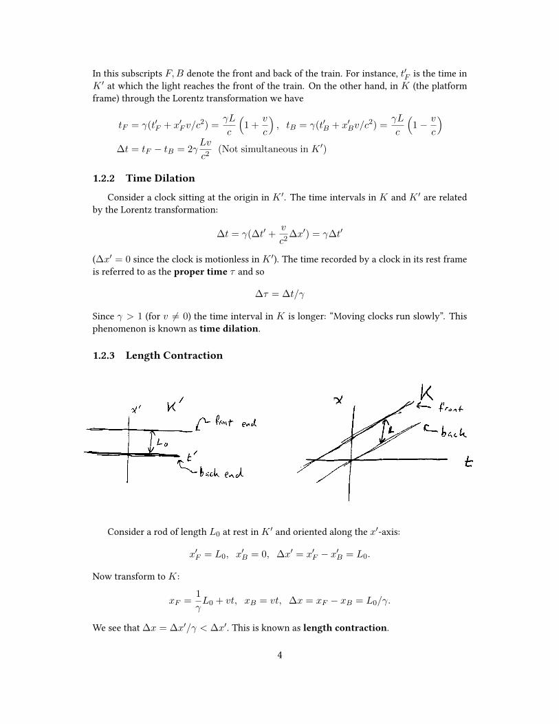
1.2.3 Length Contraction
6
7
Consider a rod of length L0 at rest in K ′ and oriented along the x′-axis:
x′F = L0, x′B = 0, ∆x′ = x′F − x′B = L0.
Now transform to K :
xF =1
γL0 + vt, xB = vt, ∆x = xF − xB = L0/γ.
We see that ∆x = ∆x′/γ < ∆x′. This is known as length contraction.
4
1.3 Relativistic Addition of VelocitiesConsider a particle moving at velocity w in K ′: dx′/dt′ = w. What is the particle’s
velocity u = dx/dt as measured in K? In Newtonian physics, the result is
u = v + w.
On the other hand, by taking the dierential of the Lorentz transformation, we have
dx = γ(dx′ + vdt′) = γdt′(w + v)
dt = γ(dt′ + vdx′/c2) = γdt′(1 + vw/c2).
Dividing these equations gives
u =dx
dt=
v + w
1 + vwc2. (4)
This gives the correct way to add velocities in special relativity. In comparing this with theNewtonian result, we see that the denominator serves to enforce the speed limit of light.Note that this formula will be modied if the particle is not moving along the x′-axis. Asour derivation did not rely on w being constant, Eq. 4 is true even if the particle in K ′ isaccelerating.
Eq. 4 can also be arrived at by considering a combination of Lorentz boosts. Take refer-ence frame K and K ′ to be as before. Now consider a third frame K ′′ in which the particlediscussed previously is at rest. That is, the origin of K ′′ is moving away from the origin ofK ′ at velocity w along the x′-axis. Now dene the rapidity ψv through
v
c= tanh(ψv)
with analogous relations for ψu and ψv .Then the matrix which transforms or “boosts” (ct, x) to (ct′, x′) is (compare to Eq. 2)
λ(v) ≡(
γ −γ vc−γ vc γ
)=
(cosh(ψv) − sinh(ψv)− sinh(ψv) cosh(ψv)
)= e−σψv (5)
where σ =
(0 11 0
)(check). In this we take the exponential of a square matrix A to be
dened through eA =∑∞
n=0An
n! . Writing the Lorentz boost in such a way enables us to nda simple way to evaluate combinations of boosts. The boost from K to K ′′ is given by
1.4 Relativistic AccelerationNow we move on to nd how to transform a particle’s acceleration between inertial
reference frames. We start by taking the dierential of Eq. 4 (recall that u = dx/dt andw = dx′/dt′):
du =1
γ2
1
(1 + vwc2
)2dw.
Next, take the dierential of an equation from our Lorentz transformation:
dt = γ(dt′ +v
c2dx′) = γ(1 +
vw
c2)dt′.
Dividing these equations gives
du
dt=d2x
dt2=
1
γ3
1(1 + vw
c2
)3 d2x′
dt′2
which relates d2xdt2
and d2x′
dt′2 .
Example: The relativistic rocket. We consider a passenger aboard a rocket who always“feels” a constant acceleration a = d2x′
dt′2 . What is the rocket’s velocity u(t) measured inthe K frame?We take the inertial frame K ′ to be moving away from the origin of K with the samespeed as the rocket at a particular time (a momentarily comoving frame – more on thislater). Then at this particular time, u = v and w = 0. This gives a dierential equationfor u:
du
dt=
(1−
(uc
)2)3/2
a.
For simplicity, let’s assume the rocket starts from rest: u(0) = 0. Solving this dieren-tial equation gives
u(t) =at√
1 +(atc
)2 .This expression gives very sensible results in limiting cases. For short times, u ≈ at asin Newtonian physics, while for long times, u ≈ c.
1.5 Relativistic Energy and MomentumWe now move on to generalise the familiar expressions of energy and momentum from
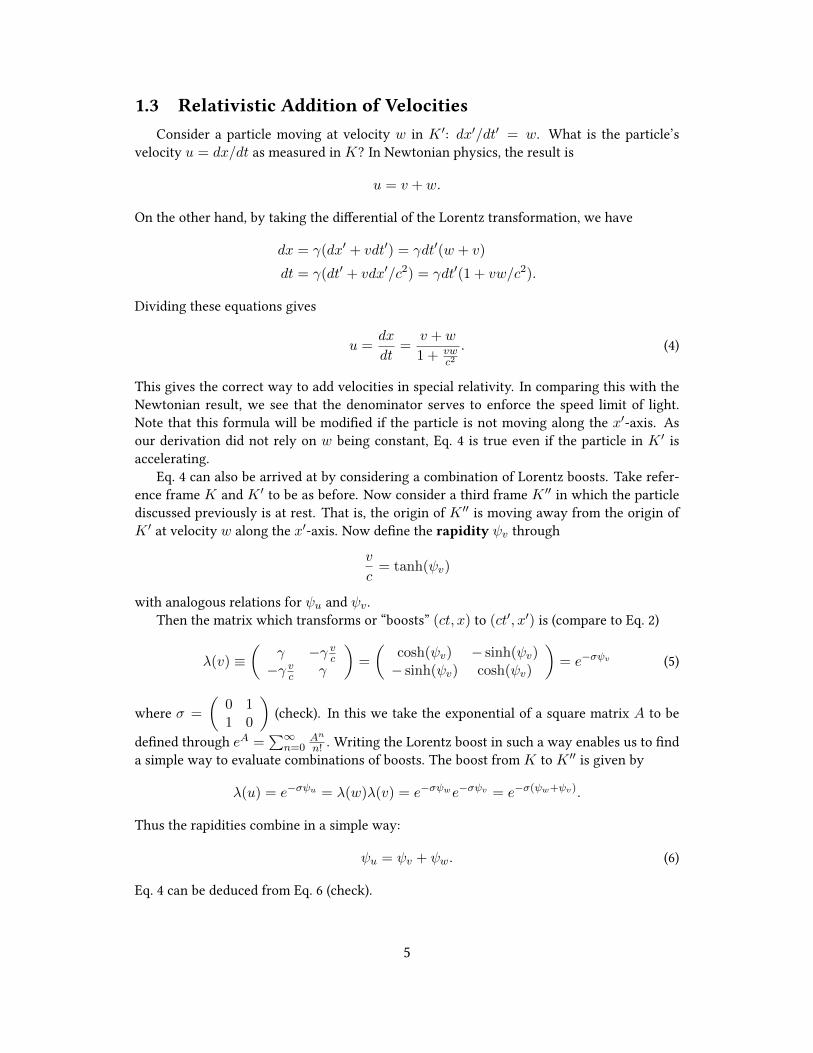
Newtonian physics to special relativity. We will motivate this by considering a collision indierent inertial reference frames. We use the frames K and K ′ as described in Sec. 1.1. InK ′, two particles, each of mass m, moving with opposite velocities collide to form a particleof mass M . In K , one of these particles is motionless (see gure).
6
Let’s rst look at this collision using Newtonian mechanics. Here, we will have M = 2mand u = 2v. In both frames mass and momentum are conserved:
frame K ′: 2m = M (Mass)
mv −mv = M · 0 (Momentum)
frame K: 2m = M (Mass)
mu = Mv (Momentum)
However, in special relativity, through the velocity addition result, we have
u =w + v
1 + wvc2
=2v
1 + (v/c)2. (7)
With this, the Newtonian momentum conservation equation inK does not hold: mu 6= Mv.This motivates us to consider the case where mass depends on velocity by the replacement
m→ f(v)mwhere f(v) is some function to be determined. With this replacement and takingf(0) = 1 we have
frame K ′: 2mf(v) = M (Mass)
f(v)mv − f(v)mv = M · 0 (Momentum)
frame K: mf(u) +m = Mf(v) (Mass)
mf(u)u = Mf(v)v (Momentum)
Solving the equations inK for f(u) gives f(u) = v/(u−v). Combining this with Eq. 7 givesf(u) = 1/
√1− (u/c)2. So we see that f(u) is nothing other than the relativistic factor:
f(u) = γ(u).We should check that all these equations are satised with this choice for f . This is easiest
to do by utilising the rapidities introduced earlier. Here we will have ψu = ψv + ψv = 2ψv .The mass equation in frame K ′ gives M = 2m cosh(ψu/2).1 Inserting this value into the
1Note that the relativistic factor of a particle moving at velocity v is γ(v) = cosh(ψv)
7
equations in K we nd the following identities:
cosh(ψu) + 1 = 2 cosh2(ψu/2)
sinh(ψu) = 2 sinh(ψu/2) cosh(ψu/2)
so everything checks.We say a particle with rest massmmoving at velocity v has a relativistic mass γ(v)m.
We further dene the relativistic momentum to be p = γ(v)mv. Extending this to severalcomponents we have
p = γ(v)mv (8)
where v = dr/dt. With these revised expressions, we have that momentum and mass areconserved in the above collision. We further interpret the conservation of mass as conserva-tion of energy. Multiplying the relativistic mass by c2 (to obtain correct units) we dene therelativistic energy to be
E = γ(v)mc2. (9)
This interpretation becomes quite plausible for v/c 1. In this regime we have
E ≈ mc2 +1
2mv2.
The second term in the above is the Newtonian kinetic energy.
1.6 A More Systematic NotationWe will now introduce some terminology and a more systematic notation which will be
used in general relativity. We label spacetime coordinates as follows:
x0 = ct x1 = x x2 = y x3 = z
(the superscripts here are not to be confused with exponents). We thus label an event by2
xµ = (ct, x, y, z) = (ct, r).
It also proves convenient to use the Einstein summation convention. With this conven-tion, summation is implied in an expression when an index appears twice. For instance,
XµYµ ≡3∑
µ=0
XµYµ = X0Y0 + . . .+X3Y3.
We will later discuss the relevance of superscript and subscript indices. Suppression of thesummation symbol often proves to be economical, but we must be careful not to write am-biguous expressions.3
2This equation may appear a little sloppy. Strictly speaking, xµ are the components of the spacetime point. Suchexpressions are common in GR.
3For instance, we might be tempted to write (XµYµ)2 = XµYµXµYµ but this in not correct. Instead, we need
to introduce another index: (XµYµ)2 = XµYµXνYν .
8
We next introduce the Minkowski metric:
ηµν =
1 0 0 00 −1 0 00 0 −1 00 0 0 −1
. (10)
This gives us a way of taking “dot products” of spacetime vectors. The spacetime line elementds is dened through
The line element is invariant under our Lorentz transformation. In fact (ds)2 is invariantunder all Lorentz transformations (think about, say, boosts in the y and z directions). In Eq.12 we have placed primes on indices to denote that these quantities are in the K ′ referenceframe. This is known as the kernel-index convention.
Now let’s introduce a more compact notation for Lorentz transformations:
dxµ′
= Λµ′νdx
ν .
For instance, for the Lorentz transformation we have been regularly using, Λµ′ν is the matrix
appearing in Eq. 2. Inserting this into the spacetime line element and demanding that thisquantity is invariant gives
ηµν = Λσ′µησ′ρ′Λ
ρ′ν (13)
or in matrix form
η = ΛT ηΛ. (14)
We take this condition as the dening relation for Lorentz transformations. More precisely,the a transformation dxµ′ = Λµ
′νdxν is a Lorentz transformation if and only if Λ satises
Eq. 13. It can be veried that the collection of matrices satisfying Eq. 14 form a group undermatrix multiplication. This group is known as the Lorentz group.
Suppose that two vectors transform under a Lorentz transformation as Xµ′ = Λµ′νXν
and Y µ′ = Λµ′νY ν . By using Eq. 14 it follows that
XµY νηµν = Xµ′Y ν′ηµ′ν′ .
9
So we see that this “dot product” is invariant. This is analogous to the way the dot productof two Cartesian vectors is invariant when they are rotated about the origin, since rotationmatrices are orthogonal. However, unlike Cartesian vectors, the dot product of Xµ withitself can be negative. Xµ is a timelike, spacelike, or null vector if XµXνηµν is positive,negative, or zero respectively.
1.7 Momentarily Comoving Reference FrameFor a particle moving at constant velocity, we can transform to an inertial frame in which
the particle is always at rest. What about an accelerating particle? For this, we introduce theMomentarily Comoving Frame (MCF) which is an inertial frame in which the particle ismomentarily at rest. Let’s revisit the line element (ds)2. Let K ′ be a MCF of the particle.Then at the moment the particle is at rest we have
where dτ is the dierential of the particle’s proper time (the proper time is the time a clocktravelling with the particle would keep). So we have the important relation
(ds)2 = c2(dτ)2. (15)
This holds even if the particle is accelerating.Let’s revisit time dilation. We can rewrite Eq. 15 as
(c2 − v2)(dt)2 = c2(dτ)2
where v2 = drdt ·
drdt . Then we can compute a proper time interval as
∆τ =
∫ tf
ti
dt√
1− (v/c)2
where ti and tf denote the initial and nal times in frame K . Note that this reduces to ourprevious result ∆τ = ∆t/γ when v is constant.
1.8 Four-Velocity and Four-MomentumDividing Eq. 15 by (dτ)2 we obtain
uµuνηµν = c2
where
uµ =dxµ
dτ.
is the four-velocity. The four-momentum of a massive particle is dened as
pµ = mdxµ
dτ.
10
Note that pµpνηµν = m2c2. We see that these are both timelike vectors.Since dxµ′ = Λµ
′νdxν and dτ is invariant, we have that the four-velocity and four-
momentum transform simply under a Lorentz transformation: uµ′ = Λµ′νuν , pµ′ = Λµ
′νpν .
This is a primary reason for why it is often best to work with these four vectors. Note, forinstance, that the coordinate velocity dr/dt does not transform in such a simple way.
Consider a particle moving with velocity v along the x-axis of K . Now let’s considerboosting to a MCF. In this frame, all components except for the 0-component of pµ′ will bezero. Using Eq. 15 we nd
pµ′
= (mc, 0, 0, 0).
Next, let’s transform back to K :
pµ = (γmc, γmv, 0, 0) = (E/c, p, 0, 0)
where p = γmdx/dt is the relativistic momentum introduced earlier.The above argument can be repeated for a particle moving in an arbitrary direction. One
nds
pµ = (E/c,p). (16)
For the four-velocity, one similarly nds
uµ = (γc, γv). (17)
The four-momentum is very useful since it combines our conserved quantities into a singlevector. Conservation of energy and momentum can be expressed simply as
dpµ
dτ= 0.
Inserting Eq. 16 into our condition pµpνηµν = m2c2 gives an expression for the relativis-tic energy
E =√
(mc2)2 + (pc)2 (18)
(compare to Eq. 9). For pcmc2 1 we have
E ≈ mc2 +p2
2m
where the second term, again, is the Newtonian kinetic energy.
1.9 Photons and the Doppler EectPhotons are particles (or quanta) of light. They have zero mass. From Eq. 18, we see that
we can express the energy of a photon as E = pc. Using Eq. 16, we see that
pµpνηµν = 0.
11
So the four-momentum of a photon is a null vector. Also, by considering Eq. 17, we see thatthe four-velocity of a photon is ill-dened (instead we take a m→ 0, v → c limiting case ofthe four-momentum).
Borrowing a basic result from modern physics, the energy of a photon is given byE = hνwhere h is Planck’s constant and ν is the photon’s frequency (units of inverse time). Thephoton’s wavelength λ satises λν = c. How does the photon’s wavelength change whenviewed from a dierent reference frame (as shown in the drawing)?
Lecture 5 (21/1/14)
19 20
In frame K , the photon’s four-momentum is
pµ = (E/c,p) =
(h
λ,h
λx
).
Now transform to frame K ′:
pµ′
=
(h
λγ(1− v/c), h
λγ(1− v/c)x
)≡(h
λ′,h
λ′x
).
The observer in frame K ′ will therefore detect a photon of wavelength
λ′ =
√1 + v/c
1− v/cλ.
When λ′ > λ we say that the photon is redshifted while if λ′ < λ we say the photon isblueshifted. Similar expressions can be derived for the photon’s frequency and energy.
We can arrive at this result in a more elegant way by considering the following. The four-velocity of the observer in the observer’s rest frame (or a MCF if the observer is accelerating)is (uµ
′)obs = (c, 0, 0, 0). We note with the above that
pµ′(uν
′)obsηµ′ν′ =
hc
λ′.
But noting the transformation properties of these four-vectors, a very similar result will holdin frame K (or any inertial frame)
pµ(uν)obsηµν =hc
λ′=
hc
λobs(19)
where λobs = λ′ is the observed value for the photon’s wavelength. So instead of transform-ing the photon’s four-momentum to the rest frame of the observer, we could just directlyevaluate the above. In practice, this is often the simplest way to proceed. Note Eq. 19 willhold even if the observer is accelerating.
12
1.10 Final Examples from Special Relativity1.10.1 Uniformly Accelerating Particle Parametrised by Proper Time
We take the position of the particle (conned to the x-axis) to be given by
x(t) =c2
a
√1 + (at/c)2.
Note that dxdt = at√
1+(at/c)2gives the result we found previously for the relativistic rocket.
Using (ds)2 = c2(dτ)2 we nd
c2(dτ)2 = c2(dt)2 − (dx)2 =c2
1 + (at/c)2(dt)2.
So
τ =
∫dt√
1 + (at/c)2=c
asinh−1(at/c) + const.
Setting the integration constant to zero so that τ = 0 when t = 0, we nd that the particle’strajectory or world line parametrised by τ is given by
xµ =
(c2
asinh(aτ/c),
c2
acosh(aτ/c), 0, 0
).
As a check, we can evaluate the particle’s four-velocity and verify uµuνηµν = c2.
1.10.2 Rindler Coordinates
Up until now, we have been treating the rocket essentially as a point particle. Our aimhere is to nd a coordinate system which is glued to the moving rocket (do not worry if thisexample is confusing at rst or second pass). We continue to take all motion to be connedto the x-axis.
First, let’s consider the following: suppose that we take all components of the rocket tobe accelerating with the same uniform acceleration. For instance, we take the trajectory ofthe front and back of the rocket to be given by
xF (t) =c2
a
√1 + (at/c)2 +
(xF −
c2
a
)xB(t) =
c2
a
√1 + (at/c)2 +
(xB −
c2
a
)so that at t = 0, xF = xF and xB = xB . By dierentiating these relations, we nd theexpected results for uniform acceleration. Now we note that at all times the rocket will havethe same length xF (t) − xB(t) = xF − xB in the K frame. But from our considerations oflength contraction, we expect that this rocket will be stretched out in its rest frame (if we candene such a thing!).
13
We instead seek a way to accelerate the rocket as a rigid object.4 First, let’s consider thetrajectory from the previous example: x(t) = c2
a
√1 + (at/c)2. This satises
x2 − c2t2 = X2a
where Xa ≡ c2/a. Through our Lorentz transformation we also nd
x′2 − c2t′2 = X2a . (20)
Now consider the following. Take the front and back of the rocket to have dierent uni-form accelerations with aF < aB (so that it maintains a constant rest length we want toaccelerate the front less than the back). Let’s further take the trajectories of the front andback to be given by
x2F − c2t2 =
(c2
aF
)2
= X2aF
x2B − c2t2 =
(c2
aB
)2
= X2aB.
Then at t = 0 both front and back ends of the rocket will be at rest with xF = XaF , xB =XaB , and xF − xB = XaF − XaB . Now consider transforming to frame K ′ through Eq.20. At time t′ = 0, we see that the rocket is at rest in this frame and will have the same restlength: x′F = XaF , x′B = XaB , and x′F − x′B = XaF −XaB . Thus, we have found a way toaccelerate the front and back of the rocket so that the the rest length of the rocket is xed. Infact, we can determine the acceleration of any intermediate point within the rocket in such away. For instance the centre of the rocket will accelerate with uniform acceleration aC givenby 1/aC = (1/aF + 1/aB) /2.
With such considerations, we see that the family of trajectories
x2 − c2t2 = X2 (21)
(for dierent X values) will describe how to accelerate the rocket as a rigid object. Addition-ally, X will give the position in a coordinate system glued to the accelerating rocket. FromX = c2/a we can read o how fast we need to accelerate this point so that the whole rocketaccelerates as a rigid object.
We therefore take X to label position in the rocket’s frame. What about time? Eq. 21 issuggestive. Suppose we choose a time coordinate T such that
t =1
cX sinh(aBT/c).
Then x = X cosh(aBT/c) (this satises Eq. 21). From the previous example, we identify T asthe time kept by a clock sitting at the back of the rocket. This is a sensible time coordinate but
4 But can rigid objects actually exist in relativity? For instance, if you push on one end of a rigid rod, and theother end moves instantly, then information would be propagated faster than the speed of light. The concept ofrigidity was debated in the early days of relativity by some eminent gures. To be more precise, in this section, weare taking the rod to be rigid in the sense of "Born Rigididy". For a discussion see arXiv:1105.3899.
14
we could have put the clock somewhere else in the rocket. Note that clocks sitting at dierentpositions in the rocket will tick at dierent rates. X and T are called Rindler coordinates.
For a massive particle under no external forces we have dpµ/dτ = 0 in an inertial frame.In the Rindler Coordinate system this reads (with some work)
d2T
dτ2+
2
X
dX
dτ
dT
dτ= 0
d2X
dτ2+(aBc
)2X
(dT
dτ
)2
= 0.
Solving these equations would give, say, the trajectory of a ball dropped in the rocket asseen from inside the rocket. The ball will fall as if it is under a gravitational eld. In ourinvestigation of general relativity, we will look at similar systems of equations in non-inertialreference frames with one important dierence: unlike the above, the gravitational elds inGR cannot be removed everywhere with a coordinate transformation.
This completes our overview of special relativity.5
5There’s a neat game which allows you to “experience” special relativity including Lorentz contractions andred/blue shifts at http://gamelab.mit.edu/games/a-slower-speed-of-light/.
2.1 The Equivalence Principle and What’s AheadLet’s consider the following thought experiment. Consider two lifts. One is deep in outer
space, while the other is freely falling under the earth’s gravitational eld. A passenger isaboard one of the two lifts. By doing experiments over small regions of spacetime the passen-ger cannot discern between the two scenarios. That is, the passenger would feel weightlessin both lifts. The passenger could do local kinematic experiments and observe that Newton’srst law is obeyed for either case.6 This is due to the equivalence of gravitational and inertialmass. This is summarised by the equivalence principle:
• In a freely falling laboratory occupying a small region of spacetime, special relativityholds.
When gravitational elds are present, it is generally not possible to nd a coordinatesystem which is inertial everywhere. In general relativity, gravity is accounted for by thecurvature of spacetime. Free particles follow the straightest possible paths in this curvedspacetime. From our discussion of special relativity, we have the line element and the equa-tions of motion of a massive particle under no forces are given by
(ds)2 = ηµνdxµdxν ,
d2xµ
dτ2= 0.
We will nd that these equations generalise to
(ds)2 = gµνdxµdxν ,
d2xµ
dτ2+ Γµνσ
dxν
dτ
dxσ
dτ= 0
(gµν and Γµνσ to be dened soon).
2.2 General Coordinate Systems for Euclidean spaceBefore jumping into our discussion of dierentiable manifolds, we will start with some-
thing more familiar: three-dimensional Euclidean space. We will nd that many of the resultsfrom Euclidean space will carry over naturally to the general case. We will start labeling in-dices with letters near the beginning of the alphabet a, b, c, d, . . . (hopefully we will not needto go too far into the alphabet!). We will reserve Greek indices for spacetime.
2.2.1 General Basis Vectors
Let
(x, y, z) = (x1, x2, x3)
6On the other hand, over larger regions of spacetime the passenger would be able to discern between the twolifts. For instance, if the lift is falling under the earth’s gravitational eld, since the gravitational eld is radial, thehorizontal distance between two balls released from rest from the left and right hands of the passenger will eventuallydecrease in apparent violation of Newton’s rst law. The balls would keep a constant horizontal separation for thelift deep in space.
16
be the usual Cartesian coordinates and
(u, v, w) = (u1, u2, u3)
be an arbitrary coordinate system. We will restrict our attention to cases where the Cartesiancoordinates can be written as functions of the (u, v, w) coordinates and vice versa. Write
r = x(u, v, w)x + y(u, v, w)y + z(u, v, w)z
and consider the vectors
e1 =∂r
∂u, e2 =
∂r
∂v, e3 =
∂r
∂w
or, more succinctly,
ea =∂r
∂ua.
These vectors are not necessarily mutually orthogonal or normalised. Now consider anothercollection of vectors dened by
e1 = ∇u, e2 = ∇v, e3 = ∇w
or ea = ∇ua. In this,∇ = x ∂∂x + y ∂
∂y + z ∂∂z is the usual gradient operator. Note we need to
write the ua coordinates as functions of the Cartesian coordinates to evaluate the above.We will now establish a useful relationship between these vectors:
ea · eb = ∇ua · ∂r∂ub
=∂ua
∂x
∂x
∂ub+∂ua
∂y
∂y
∂ub+∂ua
∂z
∂z
∂ub=∂ua
∂xc∂xc
∂ub=∂ua
∂ub
In these manipulations, we have made use of the chain rule. We have found the orthogonalityrelation
ea · eb = δab
where δab is the Kronecker delta function: δab = 1 if a = b, δab = 0 if a 6= b. Thisorthogonality relation can be used to establish the linear independence of e1, e2, e3. Thatis, consider c1, c2, c3 which satisfy
c1e1 + c2e
2 + c3e3 = 0.
Taking the dot product of this equation with ea, and using the orthogonality relation will givec1 = c2 = c3 = 0. A similar argument can be used to establish that e1, e2, e3 are linearlyindependent. We will call e1, e2, e3 the natural basis and e1, e2, e3 the dual basis.
A general vector X in Euclidean space can therefore be written in either basis:
X = Xaea = Xaea.
(summation implicit). We callXa the contravariant components ofX andXa the covariantcomponents of X. Using this orthogonality relation, the components of X can be extractedas:
ea ·X = ea ·Xbeb = Xbδ
ba = Xa.
Similarly, Xa = ea ·X.
17
2.2.2 The Metric
We dene the metric gab as
gab = ea · eb.
Similarly, we dene gab = ea · eb. From these denitions, we see that these quantities aresymmetric: gab = gba, gab = gba. Now consider two arbitrary vectors, X and Y which canbe written as
X = Xaea = Xaea
Y = Y aea = Yaea.
There are four ways we can write the dot product of these vectors:
X ·Y = gabXaY b = gabXaYb = XaYa = XaY
a.
Let’s consider XaYa = gabXaYb. Since this is true for arbitrary X, it must be that
Y a = gabYb.
Similarly, XaYa = gabXaY b tells us that
Ya = gabYb.
We see that the metric can be used to convert contravariant to covariant components andvice versa. We also have for arbitrary Y a,
Y a = gabYb = gabgbcYc.
Therefore,
gabgbc = δac .
That is, gab is the inverse of gab.
Example: Cylindrical coordinates. Let’s apply what we have established so far to cylin-drical coordinates. We take u = ρ,w = φ, and v = z where x = ρ cos(φ), y = ρ sin(φ).We nd (check)
e1 = cos(φ)x + sin(φ)y
e2 = −ρ sin(φ)x + ρ cos(φ)y
e3 = z
e1 = cos(φ)x + sin(φ)y
e2 = −1
ρsin(φ)x +
1
ρcos(φ)y
e3 = z
and
gab = diag(1, ρ2, 1), gab = diag(1,1
ρ2, 1).
18
2.2.3 Why Do We Need Two Types of Basis Vectors?
Why do we need two types of basis vectors? First we note that if (u, v, w) are just theCartesian coordinates, then the natural basis and the dual basis are the same: x = e1 = e1
with similar relations for the y and z basis vectors. For the Cartesian basis, we will use thenotation x = x1 = x1 with similar relations for the other vectors.
Now let’s go back to arbitrary (u, v, w). Some quantities are most naturally described bythe dual basis. For instance, consider a scalar function f(u, v, w). The gradient of this is
∇f =∂f
∂xaxa =
∂f
∂ub∂ub
∂xaxa =
∂f
∂uaea.
So we see that gradients are naturally expressed in the dual basis.On the other hand, some quantities are better described by the natural basis. Suppose we
have a curve in Euclidean space parameterised by t: r(t) = x(t)x + y(t)y + z(t)z. A vectortangent to this curve is given by
dr
dt=
∂r
∂uadua
dt= uaea
where ua ≡ dua
dt . Thus tangent vectors to curves are expressed in terms of the natural basis.
2.2.4 Arc Length
Let’s take the curve parametrised by t from the previous section and restrict t to t1 ≤ t ≤t2. Using our machinery, we see that the arc length ` of this curve is
` =
∫ t2
t1
dt
√dr
dt· drdt
=
∫ t2
t1
dt√uaubgab.
Example: Arc length of spiral. Let’s consider a curve which is naturally described incylindrical coordinates. Take a spiral with ρ = R = const, φ = t, z = t, and 0 ≤ t ≤ T .Then, using the metric from the previous example we nd (check)
` =
∫ T
0dt
√g11ρ2 + g22φ2 + g33z2 = T
√1 +R2.
2.2.5 Coordinate Transformations
We will now introduce another arbitrary coordinate system (u′, v′, w′) and consider howto transform quantities between this and the (u, v, w) coordinate system. We will refer tothese as the primed and unprimed coordinate systems. In the primed coordinate system, wend basis vectors using the same procedure as before: ea′ = ∂r
∂ua′and ea
′= ∇ua′ . Using the
chain rule, we can nd how the basis vectors transform under a change of coordinates:
ea =∂r
∂ua=
∂r
∂ub′∂ub
′
∂ua= Jb
′a eb′
19
where Jb′a = ∂ub′
∂ua is the Jacobian matrix. In a similar way, we can nd the transformationrule for ea:
ea = ∇ua =∂ua
∂xbxb =
∂ua
∂uc′∂uc
′
∂xbxb = Jac′e
c′ = Jab′eb′ .
With these coordinate systems, there are multiple ways to write a vector X
X = Xaea = Xaea = Xa′ea′ = Xa′e
a′ .
Inserting the transformation rules for the basis vectors into the above determines how thecomponents of X transform. One nds
Xa′ = Ja′
b Xb and Xa′ = Jba′Xb. (22)
Finally, we note that the chain rule gives a useful result:
Jac′Jc′b =
∂ua
∂uc′∂uc
′
∂ub=∂ua
∂ub= δab .
2.3 Surfaces in Euclidean SpaceWe will now consider surfaces in three-dimensional Euclidean space. Most of the results
for Euclidean space established previously can be seen to carry over to this case. We take thesurface to be given parametrically by
r(u, v) = x(u, v)x + y(u, v)y + z(u, v)z.
As before, we obtain the natural basis vectors e1 = ∂r∂u and e2 = ∂r
∂v . These vectors evaluatedat a particular point P on the surface are tangent to the surface at this point. The collection ofvectors tangent to the surface at P form a vector space which we denote as TP . Our vectorse1 and e2 can be taken as a basis for this tangent space.
As before, we dene the metric as gab = ea · eb. We take gab to be the inverse of gab:gacgcb = δab . Finally we take ea = gabeb (note the diculty in dening ea as we did in theprevious section). Note with this ea · eb = gacec · eb = gacgcb = δab .
Example: The unit sphere. We take the unit sphere to be parametrised by θ = u = u1,φ = v = u2 as
With these, we can evaluate the metric. The line element can be found to be
(ds)2 = dr · dr = gabduadub = (dθ)2 + sin2(θ)(dφ)2.
20
2.4 General Tensors and ManifoldsEuclidean space and two-dimensional surfaces in Euclidean space are both examples of
a more general entity called a manifold. An N -dimensional manifold is a space which islocally isomorphic to Euclidean space RN . For instance a small region about any point onthe unit sphere is locally isomorphic to R2. Points on anN -dimensional manifold are labelledby N coordinates (x1, x2, . . . , xN ) in such a way that there is a one-to-one correspondencebetween points in the manifold and coordinate values. It is not generally possible to describean entire manifold in such a way with a single set of coordinates. Taking our example of theunit sphere, there is not a one-to-one correspondence between coordinate values and pointsin the manifold at the north and south poles of the sphere. That is, when θ = 0 or θ = π, allvalues of φ describe the same point. For such situations, one needs to use multiple coordinatesystems to cover dierent regions of the manifold.
Suppose we have a region of a manifold described by two coordinate systems (x1, x2, . . . , xN )and (x1′ , x2′ , . . . , xN
′). Assuming the one-to-one correspondence described above, the xa co-
ordinates can be written as functions of the xa′ coordinates and vice versa. We can thus denethe Jacobian matrices as before: Jab′ = ∂xa
∂xb′and Ja′b = ∂xa
′
∂xbwhich satisfy, through the chain
rule, Jab′Jb′c = δac . We carry over the transformation rules for contravariant and covariant
vectors arrived at earlier to the present case: given a contravariant vectorXa and a covariantvector Ya, we have Xa′ = Ja
′b X
b and Ya′ = Jba′Yb.7
Contravariant and covariant vectors are examples of a more general quantity called a ten-sor. Suppose at a particular point in the manifold, we have Nn+m quantities that transformunder a change of coordinates as
Ta′1...a
′n
b′1...b′m
= Ja′1c1 . . . J
a′ncn J
d1b′1. . . Jdmb′m
T c1...cnd1...dm.
Then T a1...anb1...bmis a type (n,m) tensor. A tensor eld dened over some region of the manifold
associates a tensor of the same rank to every point in the region.We will only consider manifolds which have an associated metric gab (which are known
as Riemannian manifolds). We take the metric to be a type (0, 2) tensor eld. As beforewe take gab to be the inverse of gab. It can be shown (exercise) that gab is then a type (2, 0)tensor eld. As before, gab and gab can be used to raise and lower indices. For instance, for a(2, 0) tensor T ab, T abgbc = T ac (it can also be checked that these quantities have the correcttransformation properties). Also, we see that gab = δab .
Example: Take T abc to be a type (1, 2) tensor. DeneRa = T bab =∑
b Tbab. The b indices
are said to be contracted. In another coordinate system,
Ra′ = T b′a′b′ = Jb
′c J
da′J
eb′T
cde = δecJ
da′T
cde = Jda′T
ede = Jda′Rd.
So we see that Ra is a tensor. Generally, one can obtain an (n− 1,m− 1) tensor froman (n,m) tensor through contraction.
7We are being loose with terminology here. Strictly speaking, Xa and Ya are components of vectors and notvectors. This distinction is commonly dropped in textbooks on GR. We will adopt this convention and refer to Xa
itself as a contravariant vector.
21
2.5 Calculus of Variations and GeodesicsIn relativity, particles follow geodesics. A geodesic is the generalisation of the notion of a
straight line to a curved manifold. In the following, we will learn how to compute geodesics.
2.5.1 Calculus of Variations
Suppose we want to nd curves on the manifold parametrised by t, xa(t), which extremise
S[xa] =
∫ t2
t1
dtL(xa, xa, t)
subject to having xed endpoints, say x(t1) = x1 and x(t2) = x2. To do this write xa =xa + δxa where δxa(t1) = δxa(t2) = 0. We insert xa into S and expand in δxa. In order forxa to describe an extremum, the rst order term must vanish. To rst order in δxa, we have
S[xa] =
∫ t2
t1
dtL(xa + δxa, xa + δxa, t)
=
∫ t2
t1
dt
(L(xa, xa, t) +
∂L
∂xaδxa +
∂L
∂xaδxa).
Note that a summation over a is implied for the linear terms in δxa. Next, we integrate byparts to obtain
S[xa] = S[xa] +
∫ t2
t1
dt
(∂L
∂xa− d
dt
∂L
∂xa
)δxa.
We require the linear piece to vanish for arbitrary δxa. Therefore,∂L
∂xa=
d
dt
∂L
∂xa(23)
which are the Euler-Lagrange equations.
2.5.2 Geodesics
As we saw before, the length of a curve between two points P1 and P2 is
` =
∫ P2
P1
ds =
∫ t2
t1
dt√gabxaxb
The geodesics are given by the Euler-Lagrange equations of L =√gabxaxb. Before diving
into computing these, we introduce
K =1
2gabx
axb. (24)
Working with K is easier since it doesn’t involve square roots. For K we have∂K
∂xa= L
∂L
∂xa
d
dt
∂K
∂xa=
d
dt
(L∂L
∂xa
)= s
∂L
∂xa+ L
d
dt
∂L
∂xa
22
since L = dsdt = s. By the Euler-Lagrange equations for L we thus have
d
dt
∂K
∂xa=∂K
∂xa+ s
∂L
∂xa.
Now we note that we have the freedom to choose a convenient parametrisation of the curve.If we choose it to be related to s as t = αs+ β where α 6= 0 and β are constants, then s = 0.Our parameter t is then called an ane parameter. Choosing t to be an ane parameter,the Euler-Lagrange equations become
d
dt
∂K
∂xa=∂K
∂xa. (25)
This is the easiest way to proceed.Evaluating Eq. 25 with Eq. 24, gives (exercise)
xa + Γabcxbxc = 0 (26)
where
Γabc =1
2gad (∂cgbd + ∂bgcd − ∂dgbc) (27)
(we will begin using the shorthand ∂∂xa = ∂a). We will call Eq. 26 the geodesic equation.
Γabc is known as a Christoel symbol. From Eq. 27 we see that the Christoel symbols havethe symmetry Γabc = Γacb.
Example: Obtaining the Christoel symbols from the Euler-Lagrange equations. Thisexample will present a trick for determining Christoel symbols which often proves tobe the most ecient way of computing him. To be concrete, let’s focus on the case ofthe unit sphere. For this, we have
K =1
2
(θ2 + sin2(θ)φ2
).
The Euler-Lagrange equations are
θ − sin(θ) cos(θ)φ2 = 0
φ+ 2 cot(θ)θφ = 0.
By comparison with the geodesic equation, Eq. 26, we deduce that the only non-vanishingChristoel symbols are
Γθφφ = − sin(θ) cos(θ)
Γφθφ = Γφφθ = cot(θ).
We can check that direct evaluation of Eq. 27 gives the same results, but the method ofthis example is much less tedious. Also, note that we are writing Γθφφ instead of Γ1
22,etc. This helps us keep track of variables (was the x1 variable θ or φ?).
23
2.5.3 Comparison with Newtonian Mechanics
In Lagrangianmechanics, Newton’s second law is arrived at through a variational prin-ciple. The Lagrangian of a Newtonian particle under an external potential V is dened tobe the particle’s kinetic energy minus its potential energy V . For example, let’s consider aparticle in one spatial dimension. Then the Lagrangian is L = 1
2mx2 − V (x). It is readily
veried that the Euler-Lagrange equations give Newton’s second law: mx = −∂V∂x . Classical
particles move in ways which extremize the action S where S =∫ t2t1dtL .
The results of the previous section have an interesting connection with classical mechan-ics. First note thatK = 1
2drdt ·
drdt = 1
2gabxaxb is the kinetic energy (and Lagrangian) of a unit-
mass particle under no external forces moving on a manifold. Newton’s second law for thisparticle will be given by the Euler-Lagrange equations for K , Eq. 26. Conservation of energytells us that for a solution of Eq. 26 we will have E = 1
2gabxaxb = const.8 E = 1
2(ds/dt)2
then tells us that t is an ane parameter (s = 0). Thus the classical trajectories will also ex-tremize the arc length. From this, we conclude that the allowable trajectories of the classicalparticle will follow geodesics of the manifold. The allowable curves traced out by classicalparticles on a manifold are determined by the geometry of the manifold alone.
2.6 Parallel TransportLet’s start by considering surfaces in Euclidean space. Let XP be a vector tangent to the
surface at a particular point P . Now let xa(t) describe a curve on the manifold starting atpoint P at t = 0. How can we move the vector along the curve, keeping it in the tangentspace of the manifold along the curve, and also keeping it “as parallel as possible”? If ourmanifold was all of Euclidean space (and not a surface) the answer is more or less clear: wetake X to be the same at every point along the curve. However, this cannot generally beaccomplished for a surface since dierent points along the curve will have dierent tangentspaces. Instead, we take our condition for parallel transport to be
P · dX(xa(t))
dt= 0 (28)
where P = eaea = eaea projects into the tangent space.9 Note that dea/dt need not be in
the tangent space. We also require that X always is in the tangent space along the curve:P ·X = X. From Eq. 28 one nds that
Xa + ΓabcXbxc = 0 (29)
8We can arrive at conservation of energy directly from the Euler-Lagrange equations. Taking the time derivativeof K ,
dK
dt=∂K
∂xaxa +
∂K
∂xaxa =
d
dt
(∂K
∂xa
)xa +
∂K
∂xaxa =
d
dt
(∂K
∂xaxa)
so ddt
(∂K∂xa x
a −K)
= 0. We can verify that K = ∂K∂xa x
a −K .9 Notice the absence of the dot product in the denition of P . P dotted with a vector on either the left or right
produces another vector. P is a projector since P · P = P . Also, note for any vector Y in the tangent space at aparticular point, P ·Y = Y. Also, for a vector n normal to the surface, P · n = 0.
24
where Γabc = ea · ∂bec.We need to check that Γabc is consistent with our previous denition. First we lower the
a superscript: Γabc = gadΓdbc = ea ·∂bec. Then using ∂aeb = ∂a∂br = ∂b∂ar = ∂bea one can
verify that
Γabc = ea · ∂bec =1
2(∂b(ea · ec) + ∂c(ea · eb)− ∂a(eb · ec))
=1
2(∂bgac + ∂cgab − ∂agbc) .
So
Γabc = gadΓdbc =1
2gab (∂cgbd + ∂bgcd − ∂dgbc)
which is consistent with our previous denition.We arrived at Eq. 29 by considering surfaces, but we take it to extend to arbitrary mani-
folds. We call it the parallel transport equation.Parallel transport will give us a way of characterising the curvature of a manifold. For a
at manifold, you would imagine that a vector parallel transported about a closed loop wouldproduce the same vector. For a curved manifold, this isn’t the case.
It is also interesting to consider the special case of the parallel transport equation, Eq. 29,where Xa is a vector tangent to the curve: Xa = dxa
dt . Then the parallel transport equationreduces to the geodesic equation. That is, the tangent vector xa is parallel transported alonga geodesic. This gives an alternative way of thinking about geodesics.
Example: Parallel transport for the unit sphere.10 Consider parallel transporting avector along the curve θ = const, φ = 2πt for 0 ≤ t ≤ 1. For simplicity, we takethe curve to reside in the northern hemisphere: ω ≡ cos(θ) > 0. What is the anglebetween the initial and nal vectors?Using the Christoel symbols obtained from a previous example, we nd the paralleltransport equations
Xθ − sin(θ) cos(θ)Xφφ = 0
Xφ + cot(θ)Xθφ = 0
These have the solution
Xθ = A cos(ωφ) +B sin(ωφ)
Xφ =−A
sin(θ)sin(ωφ) +
B
sin(θ)cos(ωφ)
where A and B are constants. The initial vector at t = 0 will x A and B.The angle α between the initial nal vectors is given by
2.7 Covariant DierentiationWe want to dene a sensible way of dierentiating tensor elds which results in tensor
elds. For instance given a contravariant vector eldXa, we want some dierential operator∇a such that∇bXa is a type (1, 1) tensor eld. First let’s consider regular partial dierenti-ation. We nd that ∂bXa transforms as
∂bXa = Jc
′b J
ad′∂c′X
d′ + Jc′b J
ac′d′X
d′
where we dene Jab′c′ = ∂2xa
∂xb′xc′. Due to the presence of the last term in the above we see
that ∂bXa is not a tensor. This result is perhaps not surprising since when investigating thechange of a vector, one must account for changes both in the components and basis vectors.
We continue looking for a suitable dierential operator. Let’s reinstate basis vectors andconsider
∂bX = ∂bXaeb +Xa∂bea.
Since ∂aeb may have components not in the tangent space, let’s project these out (like in thesection on parallel transport). This gives
P · ∂bX = (∇bXa)ea.
where
∇bXa = ∂bXa + ΓabcX
c. (30)
Let’s check the transformation properties of∇bXa. Start in the primed coordinate systemand transform back:
Dotting the far left and far right expressions in this equation with ee′ gives
(∇b′Xe′) = Jcb′(ee′ · ed)(∇cXd).
Note that ee′ · ed = ee′ · ef ′Jf
′
d = Je′d . Using this, and relabelling indices, we see that
∇b′Xa′ = Jcb′Ja′d ∇cXd.
So ∇bXa is a type (1,1) tensor! Eq. 30 tells us how to take the covariant derivative of acontravariant vector eld.
What about other types of tensors? In extending this to arbitrary tensors, we require thecovariant derivative to
1. obey the Leibniz rule (aka product rule)2. reduce to partial dierentiation when acting upon a scalar eld3. be a linear operation4. result in tensor elds
26
In the second condition, we take a scalar eld to be a type (0, 0) tensor eld. Let’s applythese conditions to determine the covariant derivative of a covariant vector eld. Take Y a andZa to be arbitrary tensor elds. Note that Y aZa is an invariant scalar eld since it transformstrivially under a change of coordinates. By the second condition,∇b(Y aZa) = ∂b(Y
aZa).Then using the rst condition,
(∇bY a)Za + Y a(∇bZa) = (∂bYa)Za + (Y a∂bZa).
Finally using Eq. 30, we nd
Y a(∇bZa − ∂bZa + ΓcbaZc) = 0.
This holds for arbitrary Y a. Therefore,
∇bZa = ∂bZa − ΓcbaZc.
So we have learned how to compute the covariant derivative of covariant vectors.This procedure can be repeated for more complicated tensors. For instance, for a type (2,2)
tensor eld T abcd we consider ∇e(T abcdXaYbUcW d) = ∂e(T
abcdXaYbU
cW d) for arbitraryX,Y, U,W vectors to nd (after much algebra)
∇eT abcd = ∂eTabcd + ΓaefT
fbcd + ΓbefT
afcd − ΓfecT
abfd − ΓfedT
abcf .
The general pattern is clear.Let’s consider the covariant derivative of some familiar tensors. First, the metric tensor.
Then using expressions for the Christoel symbols in terms of the metric tensor, we nd
∇agbc = 0.
This result will greatly simplify calculations. Next, let’s consider the Kronecker delta, whichis a (1,1) tensor. Using our rules, one nds
∇aδbc = 0.
Example: Simplify gbc∇aRbc whereRbc is a tensor eld. Using the above relations, wend gbc∇aRbc = ∂aR where we note that R ≡ Raa is a scalar eld.
2.8 Geodesics in SpacetimeWe will now take a short break from tensor mathematics since we already have enough
to tell half of the story. The line element of a massive particle in special relativity, (ds)2 =ηµνdx
µdxν = c2(dτ)2, generalises naturally in general relativity as (ds)2 = gµνdxµdxν =
c2(dτ)2. We see that the proper time τ is an ane parameter. Particles in general relativity
27
under no external forces are taken to follow spacetime geodesics. So given a metric, since τis ane, we have that a massive particle will satisfy the equation
d2xµ
dτ2+ Γµνσ
dxν
dτ
dxσ
dτ= 0.
The denitions we had before for timelike, spacelike, and null vectors generalise similarly byreplacing ηµν → gµν . A photon’s four-momentum will still be a null vector.
In this section, we will check that the above requirement, that particles follow spacetimegeodesics, is a sensible one. In particular, we will check that the geodesic equation reduces toNewton’s second law for a particle under a gravitational eld in the limit where relativisticeects are small. Before doing this, we will give a short overview (or review) of Newtoniangravitation.
2.8.1 Newtonian Gravitation
We take ρ(r) to give the mass-density of some distribution of matter. The gravitationalpotential Φ(r) is related to ρ through Poisson’s equation
−→∇2Φ = 4πGρ
whereG ≈ 6.7Nm2/kg2 is the gravitational constant. To avoid confusion with the covariantderivative, we will begin using−→∇ for the gradient operator. For simplicity, we take the centreof mass of the massive object to be at the origin. We take the object to be spherically sym-metric and localised in the sense that ρ = 0 everywhere beyond some distance R. With theboundary condition Φ→ 0 as r →∞, one can solve Poisson’s equation to nd Φ(r) = −GM
rfor r > R where M is the mass of the object. A particle of mass m (take mM ) placed inthis eld will move according to Newton’s second law:
md2r
dt2= −m
−→∇Φ.
2.8.2 Weak Field Limit of the Geodesic Equation
Given a metric we can compute the equations of motion for a particle. This is analogousto the above: given Φ, we have d2r
dt2= −
−→∇Φ. We still need a generalisation of Poisson’s
equation. That is, given a mass-energy distribution, how do we compute the metric? This isthe second part of the story, which we will look at soon.
We now look at the weak-eld limit. We consider slow velocities:∣∣∣∣1c dxidt∣∣∣∣ 1
for i = 1, 2, 3. We will start using indices from the middle of the alphabet ijk . . . to denotespatial variables. We also take the metric to be time-independent and nearly at:
gµν = ηµν + hµν
where |hµν | 1.
28
Dividing c2(dτ)2 = gµνdxµdxν by (dt)2, from the slow-velocity requirement, we have
c2
(dτ
dt
)2
≈ g00c2 ≈ c2
and so dt/dτ ≈ 1 as we would expect (proper time should be close to coordinate time in thislimit). Using this and again our condition of slow velocities, we have
Γµνσdxν
dτ
dxσ
dτ= Γµνσ
dxν
dt
dxσ
dt
(dt
dτ
)2
≈ c2Γµ00.
Let’s look at these components of the Christoel symbol. Since the metric is taken to be timeindependent,
Γµ00 =1
2gµν (∂0g0ν + ∂0g0ν − ∂νg00) = −1
2gµν∂νg00 ≈ −
1
2ηµν∂νh00.
Inserting this result into the geodesic equation, we have, in this limit,
d2xµ
dτ2− 1
2c2ηµν∂νh00 = 0.
The µ = 0 equation gives d2tdτ2
= 0 which is consistent with what we found before. For thespatial components, we have
d2xi
dτ2=
1
2c2ηij∂jh00 = −1
2c2∂ih00.
Finally, using dt/dτ ≈ 1, we have
d2xi
dt2= −1
2c2∂ih00
If we identify h00 = 2c2
Φ, then this equation reproduces the Newtonian result: d2rdt2
= −−→∇Φ.
Example: Rindler coordinates. We can work out using our previous expression forRindler coordinates (dropping the B subscript) that
(ds)2 = c2(dt)2 − dx2 − dy2 − dz2 = X2( ac2
)2c2(dT )2 − dX2 − dY 2 − dZ2
where we put back in the other spatial dimensions as Y = y and Z = z.From this, we can read o the Rindler metric, gµν = diag(X2
(ac2
)2,−1,−1,−1).
Now let’s expand this metric about X = c2
a . Dene ξ through X = X + ξ and require|ξ| |X|. Then we have to rst order in ξ, gµν = ηµν + hµν where
hµν = diag(2aξ
c2, 0, 0, 0).
We thus make the identication Φ = c2
2 h00 = aξ. This is the potential for a uniformNewtonian gravitational eld (with gravitational acceleration a).
29
2.9 The Riemann Curvature TensorWe will now develop the remaining machinery we need to describe the Einstein eld
equations. Covariant derivatives, unlike partial derivatives, do not generally commute. Usingthe rules for covariant dierentiation, one nds that for a general contravariant vector eldXa (exercise),
(∇c∇d −∇d∇c)Xa = RabcdXb
where
Rabcd = ∂cΓabd − ∂dΓabc + ΓaceΓ
ebd − ΓadeΓ
ebc
is the Riemann curvature tensor.The Riemann curvature tensor satises a number of symmetries:
which are not all obvious from the above denition. We will later establish these symmetriesby using locally at coordinates. The above symmetries reduce the number of independentquantities of Rabcd to N2(N2 − 1)/12 where N is the dimension of the manifold. So, forspacetime, we have 20 independent quantities while for two-dimensions there is only one(the Gaussian curvature).
2.9.1 Parallel Transporting About Small Loops
The Riemann curvature tensor emerges naturally in the following context. Consider par-allel transporting a vectorXa about a small loop in the manifold xa(t) for 0 ≤ t ≤ T arounda point P . We ask: by how much do the initial Xa(0) and nal Xb(T ) vectors dier?
Introduce ξa through xa = (xa)P + ξa where (xa)P denotes the coordinates of the point.Generally, any quantity inside ()P , will be taken to be evaluated at P . The parallel transportequation written in integral form is
Xa(t) = Xa(0)−∫ t
0dt′Γabc(t
′)Xb(t′)xc(t′).
From this we obtain
Xa(t) = Xa(0)−∫ t
0dt′Γabc(t
′)Xb(0)xc(t′) +
∫ t
0dt′Γabc(t
′)xc(t′)
∫ t′
0dt′′ Γbde(t
′′)Xd(t′′)xe(t′′).
Everything is exact to this point. The above procedure can be repeated to generate a seriesexpansion for Xa(t). We seek an expression that is accurate to second order in distancesfrom P . To this accuracy, we can use:
Xa(t) ≈ Xa(0)−∫ t
0dt′Γabc(t
′)Xb(0)xc(t′) +
∫ t
0dt′Γabc(t
′)xc(t′)
∫ t′
0dt′′ Γbde(t
′′)Xd(0)xe(t′′).
30
Let’s work on individual terms in this expression. Put t = T . To second order accuracy:
−∫ T
0dt′Γabc(t
′)Xb(0)xc(t′) ≈ −∫ T
0dt′[(Γabc)P + (∂dΓ
abc)P ξ
d(t′)]Xb(0)xc(t′)
= −∫ T
0dt′(∂dΓ
abc)P ξ
d(t′)Xb(0)ξc(t′)
= −(∂dΓabc)PX
b(0)
∮dξcξd
∫ T
0dt′Γabc(t
′)xc(t′)
∫ t′
0dt′′ Γbde(t
′′)Xd(0)xe(t′′) ≈ (Γabc)P (Γbde)PXd(0)
∫ T
0dt′xc(t′)
∫ t′
0dt′′ xe(t′′)
= (Γabc)P (Γbde)PXd(0)
∫ T
0dt′xc(t′)(xe(t′)− xe(0))
= (Γabc)P (Γbde)PXd(0)
∫ T
0dt′xc(t′)xe(t′)
= (Γabc)P (Γbde)PXd(0)
∮dξcξe
= (Γace)P (Γebd)PXb(0)
∮dξcξd.
So we have
δXa ≡ Xa(T )−Xa(0) = (−∂dΓabc + ΓaceΓebd)P X
b(0)
∮dξcξd.
Now let’s look at fab ≡∮dξaξb. Through an integration by parts, this can be rewritten
as fab = 12
∮(dξaξb − dξbξa), from which we see that fab is antisymmetric: fab = −f ba.
Because of this, we can antisymmetrise over cd the quantity in parenthesis in the aboveexpression. The curvature tensor appears! That is, we obtain
δXa =1
2Xb(0) (Rabcd)P f
cd.
Now let’s specify a particular curve. Let’s hold constant all of our coordinates except fortwo, xc and xd. Let’s integrate counterclockwise along a rectangle centred at point P in thecd-plane. Take the width and height of this rectangle to be ∆xc and ∆xd respectively. Thenthrough Green’s theorem, we obtain
f cd = −f dc =1
2
∮(dξcξd − dξdξc) = −
∫dξcdξd = −∆xc ∆xd
where all other components of f vanish. Finally, we obtain
δXa = −Xb(0)(Rabcd
)P
∆xc ∆xd
(no summation over c and d).Thus the Riemann curvatures tensor tells us how the initial and nal vectors will dier.
We call a manifold at if the Riemann curvature tensor vanishes everywhere. Otherwise, wecall the manifold curved.
31
2.10 Locally Flat CoordinatesOur aim is to construct a coordinate system in which at a particular point P , the Christof-
fel symbols vanish and the metric tensor is the identity matrix (or the Minkowski metric forspacetime). Motivation for this includes:
• Locally at coordinates will help us establish important symmetries of the Riemanncurvature tensor
• Locally at coordinates are demanded by the equivalence principle. That is, for generalrelativity to locally reduce to special relativity, in light of the geodesic equation, wemust be able nd a frame in which the Christoel symbols vanish at an event. In thecontext of spacetime, locally at coordinates are often referred to as locally inertialframes or freely falling frames.
As we have done a couple of times before, we will consider surfaces to develop our intu-ition. Following the picture, we introduce the y-coordinates through
ya ≡ δr · (ea)P
where δr = r − (r)P . Expanding r about P we obtain δr ≈ (ea)P δxa + 1
2(∂bea)P δxa δxb
where δxa = xa − (xa)P . Then to second order in distances from P we have
ya = δxa +1
2(Γabc)P δx
bδxc.
Inverting this equation we nd
δxa = ya − 1
2(Γabc)P y
byc
which again is second-order accurate. From this we can determine an expression for theJacobian which is accurate at rst order:
∂xa
∂yb= δab − (Γabc)P y
c.
32
We use this to nd the metric in the y-coordinate system gab (we will use tildes to denotequantities in the y-coordinate system) as
gab =∂xc
∂ya∂xd
∂ybgcd ≈ gab − (Γabc)P y
c − (Γbac)P yc = gab − (∂cgab)P y
c
which is accurate at rst order. In the second equality, we have used the denition of theChristoel symbols. From this we nd(
∂gab∂yc
)P
=
(∂xd
∂yc∂gab∂xd
)P
− (∂cgab)P = 0.
Note that at point P , ∂xd∂yc = δdc . From the denition of the Christoel symbols, from this weconclude that all Christoel symbols in the y-coordinate system will also vanish at P :(
Γabc
)P
= 0.
We can go further. Let’s introduce a z-coordinate system which is related to the y-coordinate system as
ya = Sabzb.
In this, we take the components of S to be constants. We will use double-tildes to denotequantities in the z-coordinate system. For the metric tensor,
˜gab = ScaSdbgcd.
We wish to choose S such that ˜g becomes the identity matrix. Let’s proceed by writing matrixequations. Since g is a symmetric metric, we can diagonalise it with an orthogonal matrix:OT gO = D whereD is a diagonal matrix composed of the eigenvalues of g. For Riemannianmanifolds, g will have all positive eigenvalues (while for spacetime it will have one positiveand three negative). Taking all positive eigenvalues, we will have D−1/2OT gOD−1/2 = 1.We thus choose S = OD−1/2. Through the transformation rule for the Christoel symbols(practice problems), we see that the Christoel symbols will also vanish in the z-coordinatesystem.
In summary (dropping tildes and going back to xa for coordinates), for a manifold withpositive denite metric, we can nd a coordinate system which is at about a point P in thesense that
gab ≈ 1ab +1
2(∂c∂dgab)P δx
cδxd
and
(Γabc)P = 0.
Very similar arguments can be given for spacetime. Here a locally at coordinate system willgive
gµν ≈ ηµν +1
2(∂σ∂ρgµν)P δx
σδxρ
and
(Γµνσ)P = 0.
33
2.10.1 Symmetries of the Riemann Tensor
In locally at coordinates, the Riemann curvature tensor is
(Rabcd)P = (∂cΓabd − ∂dΓacb)P .
Recalling that rst-order derivatives of the metric tensor vanish at point P , we nd (check),
(Rabcd)P =1
2(∂b∂cgad + ∂a∂dgbc − ∂b∂dgac − ∂a∂cgbd)P .
In comparison with the general expression of the curvature tensor in terms of the metrictensor, the above expression is vastly simplied. From this we can directly verify the symme-tries of the Riemann curvature tensor written earlier at point P in our locally at coordinatesystem.
However, sinceRabcd is a tensor, it is enough to establish the symmetries Eq. 31 in a singlecoordinate system. For instance, we have for locally at coordinates, (Rabcd)P = −(Rbacd)P .We can use Jacobian matrices to transform to another coordinate system (which need not belocally at) and nd (Ra′b′c′d′)P = −(Rb′a′c′d′)P . The nal point to note is thatP is arbitrary.
2.11 TensorsDerived From theRiemannCurvature Tensor andthe Einstein Field Equation
For later use, we will now introduce tensors which follow from the Riemann curvaturetensor. The Ricci tensor Rab is dened as
Rab = Rcacb.
From the symmetries of the Riemann tensor (how?), we see thatRab is symmetric: Rab = Rba.The Ricci scalar R follows from the Ricci tensor as
R = Raa = gabRba.
Finally, the Einstein tensor Gab is dened as
Gab = Rab −1
2gabR.
The Einstein eld equations are
Gµν =8πG
c4Tµν
where Tµν is the energy-momentum tensor which we will look at soon. For a particularenergy momentum tensor, we solve the Einstein eld equations to determine the metric. Theanalogy with Newtonian gravity is: given a mass distribution ρ(r), we solve Poisson’s equa-tion to determine the gravitational potential. In due course we will verify that Einstein’s eldequations reduce to Poisson’s equation in the non-relativistic limit. Then with this metric,we can solve the geodesic equation to determine the trajectory of a particle in this eld. J.A. Wheeler succinctly described this process as “Spacetime tells matter how to move; mattertells spacetime how to curve.”
34
2.12 The Bianchi Identity and the Contracted Bianchi IdentityWe will need a couple more relations for the Riemann curvature tensor. The Riemann
curvature tensor satises the Bianchi identity:
∇eRabcd +∇dRabec +∇cRabde = 0. (32)
Like the symmetries of Riemann tensor established earlier, the Bianchi identity is easiest toestablish by using locally at coordinates. For such a coordinate system (since the Christoelsymbols vanish)
(∇eRabcd)P = (∂eRabcd)P = (∂e∂cΓ
abd − ∂e∂dΓacb)P .
From this, we can directly verify Eq. 32.From the Bianchi identity, we can derive the contracted Bianchi identity which reads
∇aGab = 0. (33)
First, contract a and c in the Bianchi identity to nd
∇eRbd −∇dRbe +∇aRabde = 0.
For the second term, we have used Eq. 31: ∇dRabea = ∇d(gafRfbea) = −∇d(gafRfbae) =−∇dRabae = −∇dRbe. Since ∇cgab = 0, for a tensor eld Xa we have gac∇bXa = ∇bXc.With this in mind, we can “raise indices behind the covariant derivative operator”. Raise band contract with d to nd
∇eR−∇bRbe +∇aRabbe = 0.
Let’s work on the last term on the left-hand side:
Finally, raising b we obtain∇a(Rab − 12gabR) = 0 which is Eq. 33.
35
2.13 Relativistic Fluids and the Energy-Momentum TensorThe remaining piece of Einstein’s eld equation which we need to address is the energy-
momentum tensorTµν . For most situations in this course, we will take the energy-momentumtensor for a perfect uid which reads
Tµν = (ρ+ p/c2)uµuν − pgµν .
In our discussion of special relativity, we introduced the four-velocity of a particle. We nowgeneralise uµ to a vector eld so that (uµ)P describes the average four-velocity of particlesat point P in spacetime. We take ρ to be the proper density (mass density measured in a mo-mentarily co-moving frame) of the matter. The pressure, which also can depend on positionis p. Both ρ and p are scalars.
We take the equations of motion of the relativistic uid to be given by
∇µTµν = 0.
Note the consistency between this and the eld equations as a result of the contracted Bianchiidentity. We will follow our usual practice of showing that these equations of motion reduce tosomething sensible in the non-relativistic limit. We will now work on writing these equationsof motion in a more intuitive way.
First some useful relations. Since uµuµ = c2, we have that uν∇µuν = uν∇µuν = 0. Forour perfect uid we also have Tµνuν = ρc2uµ. Multiply our equations of motion by uν (andsum as usual over ν):
To obtain our other uid equation, we use the projection tensor
Pµν = δµν −1
c2uµuν .
Note that Pµν uµ = 0 and Pµσ P σν = Pµν . This enables us to look at components of the uidequation orthogonal to the four-velocity eld. With this,
0 = P σν ∇µTµν = P σν((ρ+ p/c2)uµ∇µuν − gµν∂µp
)= (ρ+ p/c2)uµ∇µuσ − ∂µp(gµσ − uµuσ/c2).
Relabelling indices,
(ρ+ p/c2)uµ∇µuν = ∂µp(gµν − uµuν/c2). (35)
Eqns. 34, 35 give a more explicit description of the equations of motion of relativisticuids. They reduce to the continuity and Euler equations from uid mechanics11 in the non-relativistic limit. In particular, we consider the limit where ρ p/c2, gµν = ηµν , and uµ =
11A description of classical ideal uids is outside the scope of this course. If you haven’t seen these equations, Irecommend The Feynman Lectures on Physics for an accessible introduction.
36
(c,v) where v is the velocity eld of the uid. In this limit, Eq. 34 becomes (exercise)
∂tρ = −−→∇ · (ρv)
which is the continuity equation. The µ = 1, 2, 3 components of Eq. 35 become (exercise)
ρ(∂tv + (v ·−→∇)v) = −
−→∇p
which is the Euler equation.
Example: Dust in Special Relativity. A relativistic uid in the absence of pressure isreferred to as dust. In this example we will look at dust in special relativity where gµν =ηµν and hence∇µ = ∂µ. Using uµ = γ(c,v) and writing out the spatial, temporal, andmixed components of the energy-momentum tensor impels us to introduce ρ = γ2ρ.We then have
T 00 = ρc2
T 0i = T i0 = ρcvi
T ij = ρvivj
where v is the coordinate velocity (or three-velocity) eld. Note that since vi is nota tensor we have the unusual placement of indices. ρ is in fact the frame-dependentdensity of the uid. The combined eect of length contraction and relativistic enhance-ment of mass provides the factor of γ2. It can be veried that the equations of motion∂µT
µν = 0 can be written, without approximation, as (exercise)
∂tρ = −−→∇ · (ρv)
and
∂tv + (v ·−→∇)v = 0.
Unlike Eqns. 34 and 35, the above are not tensor equations. These equations provideperhaps the clearest connection with classical ideal uids.
2.14 Weak Field Limit of the Einstein Field EquationsWe need to show that the Einstein Field Equations reduce to Poisson’s equation in the
non-relativistic limit. To do this, it is helpful to write the eld equations in an alternativeway. Let κ = 8πG
c4. Then the eld equations are
Rµν − 1
2gµνR = κTµν .
Lowering ν and contracting with µ and noting that gµµ = δµµ = 4, we have
R = −κT
37
where T ≡ Tµµ. Putting this back into the eld equations we nd
Rµν = κ(Tµν − 1
2gµνT ) (36)
or, lowering indices,
Rµν = κ(Tµν −1
2gµνT ) (37)
which is an alternative way of writing the eld equations. As a special case when Tµν = 0this reduces to
Rµν = 0
which are the vacuum eld equations.We consider the limiting case of small velocities v/c 1. The metric is taken to be time
independent and nearly at: gµν = ηµν + hµν where |hµν | 1. We further require thatp/c2 ρ. With these requirements, the 00 component of the energy momentum tensor willbe dominant. We have T00 ≈ T 00 ≈ ρc2 and T = Tµµ = (ρ+ p/c2)c2− 4p ≈ ρc2. With this,we nd
R00 = κ(T00 −1
2g00T ) ≈ κ
2ρc2. (38)
Now let’s consider the 00 component of the Ricci tensor in this limit. To rst order in hµν ,
Rµνρσ = ∂ρΓµνσ − ∂σΓµνρ
and so to this order,
R00 = Rµ0µ0 = ∂µΓµ00 − ∂0Γµ0µ = ∂µΓµ00
(recall we are taking the metric to be time-independent). Recalling some results from 2.8.2,we have to rst order in hµν
R00 = ∂µΓµ00 = −1
2ηµν∂µ∂νh00 =
1
2
−→∇2h00 =
1
c2
−→∇2Φ.
Inserting this into Eq. 38 we nd Poisson’s equation:−→∇2Φ = 4πGρ.
3 General Relativity Applied
3.1 The Schwarzschild GeometryIt is now time to put the theory of general relativity uncovered during the last chapter to
work.
38
We seek to nd the spacetime metric corresponding to a spherically-symmetric massivebody of total mass M . We will solve the vacuum eld equations
Rµν = 0
which are valid outside of the massive body’s interior. We take the metric to be sphericallysymmetric, time-independent, and asymptotically at. The following ansatz satises thesethree conditions:
where we require A,B → 0 as r → ∞ so that the metric reduces to the Minkowski metricat large distances from the body.12 From this, we can compute the Ricci tensor13. One ndsthe non-vanishing components are
R00 = e2(A−B)(A′2 +2
rA′ −A′B′ +A′′)
R11 = −A′2 +2
rB′ +A′B′ −A′′
R22 = e−2B(−1 + e2B − rA′ + rB′)
R33 = sin2(θ)R22.
In the above, primes denote derivatives with respect to r. Combining the equations for R00
and R11 gives A′ +B′ = 0. Using our boundary condition then gives A+B = 0. InsertingA = −B into the equation for R22 gives
2rA′ + 1 = e−2A.
Noting that we can write the LHS of this equation as e−2A ddr (re2A), we can immediately
solve to nd re2A = r + k where k is a constant of integration. With this we have
(ds)2 = c2(1 +k
r)(dt)2 − 1
1 + kr
(dr)2 − r2(dθ)2 − r2 sin2(θ)(dφ)2.
How do we determine k? We require that the metric reduces to the correct weak-eld limit fora gravitational potential Φ(r) = −GM
r . Using results from the previous chapter, we require
g00 = 1 +k
r= 1 + h00 = 1 +
2
c2Φ(r).
We then nd k = −2MG/c2. With this value for k, we have found the Schwarzschildmetric.
12 Actually, one can arrive at this metric by starting with a general spherically symmetric metric and applyingcertain variable changes.
13Read o the metric from (ds)2. From the metric, compute the Christoel symbols. From the Christoel symbolscompute the Riemann tensor. From the Riemann tensor, compute the Ricci tensor. This is a straightforward butcomputationally intensive task and is perhaps best left to a symbolic mathematics package likeMaple orMathematica.
39
3.2 Classical Kepler MotionBefore considering motion under the Schwarzschild metric, we will rst, for comparison
and to set some notation, consider the Newtonian motion of a particle under a gravitationalpotential Φ(r) = −MG
r . We take the mass of the particle m to be much smaller than M sothat we can avoid working with “reduced masses”. That is, we can take the position of thelarger mass M to be xed in space. Newton’s second law reads
d2r
dt2= −−→∇Φ = −MG
r2r.
The angular momentum L = r×mdrdt is conserved:
dL
dt=dr
dt×mdr
dt+ r×
(−mGr2
r
)= 0.
Since L is conserved and r · L = 0, the motion will be conned to a plane. We use polarcoordinates (r, φ) for this plane.
From classical mechanics, drdt = φφ and dφdt = −φr. Using this,
d2r
dt2=
d2
dt2(rr) = (r − rφ2)r +
1
r
d
dt(r2φ)φ =
−MG
r2r.
So
r − rφ2 = −MG
r2, and
d
dt(r2φ) = 0. (39)
It is useful to introduce u = 1/r and regard r as a function of φ (compare with thecomputation of geodesics on the unit sphere). Let h = r2φ which is a constant of motion bythe above equations. Then
dr
dt=dr
du
du
dφφ = −hdu
dφ
andd2r
dt2= −hd
2u
dφ2φ = −h2u2 d
2u
dφ2
Inserting this into Eq. 39 we ndd2u
dφ2+ u =
GM
h2
which is the Binet equation. It has the solution
u(φ) =GM
h2(1 + e cos(φ− φ0)).
Where φ0 and e are constants. e is called the eccentricity. We obtain circular, elliptic,parabolic, and hyperbolic motion for e = 0, 0 < |e| < 1, |e| = 1, and |e| > 1 respectively.For instance, for φ0 = 0 and |e| 6= 1, we can write this solution as
(1− e2)
(x+
Re
1− e2
)2
+ y2 =R2
1− e2
where R = h2
GM .
40
3.3 Precision of the PerihelionWe will now consider the analogous problem in general relativity, of a massive particle
in orbit.It is convention to dene m = MG
c2. This quantity has units of length. With this, the
Schwarzschild line element is
(ds)2 =
(1− 2m
r
)c2(dt)2 −
(1− 2m
r
)−1
(dr)2 − r2(dΩ)2
where (dΩ)2 = sin2(θ)(dφ)2 + (dθ)2. This is related to the proper time dierential in theusual way for massive particles: (ds)2 = c2(dτ)2. Since τ is an ane parameter, the geodesicequation will be given by the Euler-Lagrange equations of K = 1
2gµν xµxν .
Let’s rst search for conserved quantities. Since the metric does not explicitly depend onφ or t, the corresponding Euler-Lagrange equations gives the conserved quantities
k =
(1− 2m
r
)t
h = r2 sin2(θ)φ.
Additionally, K = 12
(dsdτ
)2= 1
2c2 itself is conserved. As in the previous section, we consider
planar motion and set θ = π/2. Inserting our conserved quantities intoK and reintroducingu = 1/r (see previous section), we nd
c2k2 − h2
(du
dφ
)2
= (c2 + h2u2)(1− 2mu).
Next we dierentiate the above with respect to φ to nd
d2u
dφ2+ u =
c2m
h2+ 3mu2.
This is the relativistic Binet equation. The dierence between this and the Binet equationfrom the previous section is the last term on the right-hand side, which makes the currentequation a non-linear ode. Using the mass of the sun for M , we nd m = MG/c2 ≈ 1500m. This is well within the radius of the sun. Therefore, for typical planetary motion, um =m/r will be a small number and the last term on the right-hand side of the relativistic Binetequation can be viewed as a small correction. Its role in solar system motion is typically smallbut sometimes measurable. This term will be largest for planets close to the sun.
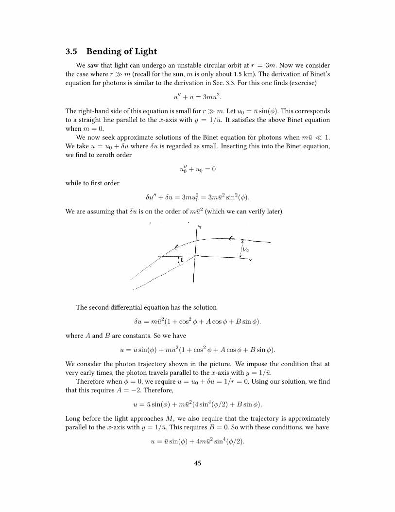
In the following we will consider nearly circular motion and write u = u0 + δu whereu0 is a constant and δu u0. Putting this into Binet’s equation, we have to zeroth and rstorder in δu,
u0 =c2m
h2+ 3mu2
0
d2δu
dφ2+ δu = 6mu0δu.
41
Solving the second equation, δu = A cos(√
1− 6mu0(φ−φ0)) whereA andφ0 are constants.So,
u = u0 + δu = u0[1 + e cos(√
1− 6mu0φ)]
where we have put φ0 = 0 for convenience.The point of closest approach to the sun is referred to as the perihelion. Unlike Kepler
motion, the above predicts that the perihelion will precess. The observation of this eect forthe planet Mercury was one of the earliest observational tests of general relativity.
Let’s take e > 0. Then the values ofφ corresponding to perihelia areφn = 2πn/√
1− 6mu0 ≈2πn(1 + 3mu0) for integer n. From this we see that after every orbit, the perihelion will ad-vance by
∆φ = 6πmu0.
Putting in approximate numbers for Mercury (89 days per orbit, 1/u0 ≈ 5.8 × 10¹⁰ m), wend that after a century its perihelion will advance by 42 arcseconds (602 arcseconds = 1).The observational value is 43.1± .5 arcseconds.14
3.4 General Orbits in the Schwarzschild GeometryWe will now broaden our discussion to include the motion of photons. From our dis-
cussion of photons in special relativity, we have the result (ds)2 = ηµνdxµdxν = (c2 −
v2)(dt)2 = 0 from the rst postulate. This result continues to hold in general relativity where(ds)2 = gµνdx
µdxν . We conclude this by appealing to locally at coordinates. That is, wecan nd a coordinate system in which gµν locally reduces to ηµν . By the equivalence prin-ciple, we can nd a frame in which special relativity locally holds. In this frame (ds)2 = 0.However, since (ds)2 is a scalar quantity, this must hold in all frames. Proper time is ill de-ned for photons. We therefore need to choose a dierent ane parameter, which we call w,with which to describe their motion.
In order to not produce fairly similar derivations for light and massive particles we writethe following:
gµν xµxν = αc2
where α = 0 and xµ = dxµ/dw for light while α = 1 and xµ = dxµ/dτ for massiveparticles. As before, for geodesic motion, we have the conserved quantities h = r2φ andk = (1 − 2m/r)t where we are still restricting to planar motion θ = π/2. Inserting theseinto the above, we obtain
1
2r2 + V (r) = E
where E = c2(k2 − α)/2 and
V (r) = −mc2
rα+
h2
2r2− mh2
r3.
14Actually, the perihelion of Mercury will also precess according to Newton’s laws. This is the result of grav-itational elds from sources other than those of Mercury and the sun. More precisely, the amount of additionaladvancement (not accounted for by Newton’s laws) is (43.1± .5) arcseconds per century.
42
r
97
91
98
99 100
Taking the derivative of the above with respect to the ane parameter we have
r = −∂rV.
The above equations describe a Newtonian particle of mass m in a potential V . Thusthe advantage of the current formulation is that we may now use all of our intuition fromNewtonian physics to understand the dynamics in at least a qualitative way. For a massiveparticle (α = 1), we have
V (r) = −mc2
r+
h2
2r2− mh2
r3.
This will have a maximum and minimum when hmc >
√12 (see picture) occurring at r+ and
r− where
r± =h2
2mc2
(1±
√1− 12
(mch
)2).
This can be contrasted with the classical problem which can have stable orbits for h 6= 0. Itcan be seen that circular orbits at r+ are stable while those at r− are unstable. That is, anysmall perturbation added to the circular orbit at r− generically will grow.
We now turn to the motion of light. For this we have
V (r) =h2
2r2− mh2
r3.
This potential has a maximum at r = 3m which corresponds to an unstable circular orbit.
Example: Proper time for orbits. Suppose we have a satellite in a circular (geodesic)orbit at radius r about a planet. What is the proper time duration (∆τ)orb for a completeorbit as measured by a passenger aboard the satellite? A second observer stays at a xedlocation in the Schwarzschild coordinate system at r (using, say, a rocket pack). Whattime does this observer measure (∆τ)obs for an orbit of the satellite?Let’s rst try to nd (∆τ)orb. For circular orbit, we have u = 1/r = const. Thus theBinet equation becomes
u =c2m
h2+ 3mu2.
43
We use h = r2φ to nd
φ2 =mc2u3
1− 3mu=
GM
r3(1− 3mr )
.
For simplicity, we take the orbit to be counter-clockwise (so φ is positive). Then candirectly integrate to nd
(∆τ)orb = 2π
√r3(1− 3m/r)
GM.
Next, let’s nd the coordinate time duration ∆t for a complete orbit. We use c2 =gµν x
µxν and put r = 0 to nd
c2 = (1− 2m/r)c2t2 − r2φ2.
Inserting the above result for φ, we nd
1 = t2(1− 3m/r).
This can be directly integrated to give
∆t =1√
1− 3m/r(∆τ)orb = 2π
√r3
GM.
In this, we have taken the positive square root so that this reduces to the correct resultin the m → 0 limit. Incidentally, this is the same result one obtains in Newtonianphysics (Kepler’s third law).Now for (∆τ)obs. This observer does not follow a geodesic. Thus we cannot use thegeodesic equation to describe his motion. However, we still may use c2 = gµν x
µxν (ourderivation of this said nothing of geodesics). Since this observer is at a xed location,we have15
c2 = (1− 2m/r)c2t2.
From this we see that
(∆τ)obs =√
1− 2m/r∆t = 2π
√r3(1− 2m/r)
GM.
Putting everything together, we see that (∆τ)orb < (∆τ)obs < ∆t.15This relation suggests that people living at lower elevations will age slower. This eect was in fact measured
by researchers at NIST using atomic clocks http://www.nist.gov/public_affairs/releases/aluminum-atomic-clock_092310.cfm
3.5 Bending of LightWe saw that light can undergo an unstable circular orbit at r = 3m. Now we consider
the case where r m (recall for the sun, m is only about 1.5 km). The derivation of Binet’sequation for photons is similar to the derivation in Sec. 3.3. For this one nds (exercise)
u′′ + u = 3mu2.
The right-hand side of this equation is small for r m. Let u0 = u sin(φ). This correspondsto a straight line parallel to the x-axis with y = 1/u. It satises the above Binet equationwhen m = 0.
We now seek approximate solutions of the Binet equation for photons when mu 1.We take u = u0 + δu where δu is regarded as small. Inserting this into the Binet equation,we nd to zeroth order
u′′0 + u0 = 0
while to rst order
δu′′ + δu = 3mu20 = 3mu2 sin2(φ).
We are assuming that δu is on the order of mu2 (which we can verify later).
Lecture 22 (3/3/14)
101 102
103 104
The second dierential equation has the solution
δu = mu2(1 + cos2 φ+A cosφ+B sinφ).
where A and B are constants. So we have
u = u sin(φ) +mu2(1 + cos2 φ+A cosφ+B sinφ).
We consider the photon trajectory shown in the picture. We impose the condition that atvery early times, the photon travels parallel to the x-axis with y = 1/u.
Therefore when φ = 0, we require u = u0 + δu = 1/r = 0. Using our solution, we ndthat this requires A = −2. Therefore,
u = u sin(φ) +mu2(4 sin4(φ/2) +B sinφ).
Long before the light approaches M , we also require that the trajectory is approximatelyparallel to the x-axis with y = 1/u. This requires B = 0. So with these conditions, we have
u = u sin(φ) + 4mu2 sin4(φ/2).
45
Now we consider the deection of light described by this equation. That is, we want todetermine ε for which u = 0. Putting u = 0 and φ = π + ε in the above equation, we nd
0 = u sin(π + ε) +mu24 sin4
(π + ε
2
)≈ −uε+mu24.
So to lowest order in mu,
ε = 4mu.
This eect, observed during a solar eclipse in 1919 by Eddington and collaborators, providedan early verication of general relativity.
3.6 Spectral ShiftIn our discussion of special relativity, we saw that the energy of photons depends on the
reference frame in which they are observed. We will now consider how gravity aects theenergy of photons.
We will derive our main result by carrying over a trick we learned back in our discussion ofspecial relativity. Take an observer with four-velocity (uµ)obs and a photon with four-velocitypµ. Suppose that the photon barely misses the observer at a particular spacetime point. Atthis event, the observer assigns energy hν = (uµ)obspµ to the photon. We established thisresult for special relativity, but, through the equivalence principle it also holds in generalrelativity. Note for our Schwarzschild coordinate system, uµ = (ct, r, θ, φ).
We now consider an emitter which emits photons of energy hνE travelling radially out-ward towards a receiver. Both the emitter and the receiver are at xed spatial coordinates inSchwarzschild spacetime. An observer at the emitter measures the energy of the photons tobe hνE . What energy, hνR, does an observer at the receiver assign to the photons?
Take the emitter to have r = rE and the receiver to have r = rR where rE < rR. Thenthe two stationary observers will have four-velocities
(uµ)E = (ct, 0, 0, 0) =
(c√
1− 2m/rE, 0, 0, 0
)
(uµ)R =
(c√
1− 2m/rR, 0, 0, 0
).
For the light, since dxµ
dw is parallel to pµ, we can choose the ane parameter w such thatpµ = dxµ
dw . Using k = (1 − 2m/r)t, and noting that the photon travels radially outward(r > 0), we have have
pµ =
(kc
1− 2m/r, kc, 0, 0
)and
pµ =
(kc,− kc
1− 2m/r, 0, 0
).
46
To nd pµ we have, as usual, used pµ = gµνpν .
Now we can directly evaluate the energies of the light as measured by observers at theemitter and receiver:
hνE = (uµ)Rpµ =kc2√
1− 2m/rE
hνR = (uµ)Rpµ =kc2√
1− 2m/rR.
Dividing these results, we arrive at the spectral shift formula
νEνR
=λRλE
=
√1− 2m/rR1− 2m/rE
For the case where the photons travel radially inwards (and rR < rE), one obtains anidentical expression (check). So we see that photons “falling” under a gravitational eld be-come more energetic (or blue shifted).
3.7 The Pound-Rebka Experiment
105
Lecture 23 (4/3/14)
106
107 108
We will now consider an example which nicely combines the Doppler shift (which we sawin special relativity) with the gravitational spectral shift. As shown in the gure, photons areemitted and travel radially inward to a receiver. Through the previous analysis, the photonswill become more energetic, or blue shifted, as they “fall” under earth’s gravitational eld (wetake M for this example to be the mass of the earth). On the other hand, when the emitteris moving radially outward with velocity v = drE
dt > 0, we expect, through the Dopplereect, that this will decrease, or red shift, the energy of the light. We ask: for which v willthe energy of the emitted and received photons (as determined by observers situated at theemitter and receiver) be the same? This result is relevant for the Pound-Rebka experiment.16
In contrast to the other “classical” tests of general relativity we discussed previously, namely16 Pound, R. V.; Rebka Jr. G. A. (November 1, 1959). "Gravitational Red-Shift in Nuclear Resonance". Physical
Review Letters 3 (9): 439
47
the bending of light and the precession of the perihelion, the work of Pound and Rebka wasterrestrial experiment: ∆r = rE − rR is the distance from the roof to the basement of abuilding.
To keep our expressions manageable, we will work to rst order inm/rE ,m/rR, and v/cwhich are all small numbers for the experiment under consideration. For the earth,m is onlyaround a centimetre. We can use our expression for (uµ)R obtained in the previous section:
(uµ)R =
(c√
1− 2m/rR, 0, 0, 0
)≈ (c(1 +m/rR), 0, 0, 0)
For the light, we have
pµ =
(kc,
kc
1− 2m/r, 0, 0
).
This is for light travelling radially inward (compare to pµ from the previous section).For (uµ)E , we have
(uµ)E = (ct, r, 0, 0).
Using r = drdτ = dr
dtdtdτ we have
(uµ)E = ct(1, v/c, 0, 0).
Using our requirement c2 = uµuµ, gives
c2 = c2t2(
1− 2m/rE −v2/c2
1− 2m/rE
)≈ c2t2(1− 2m/rE).
So t ≈ 1 +m/rE and
(uµ)E ≈ (c(1 +m/rE), v, 0, 0)
Now we these expressions for the four-vectors, we obtain
hνE = kc2(1 +m/rE + v/c)
hνR = kc2(1 +m/rR).
The energy of the emitted and received photons will be the same when
v
c=m
rR− m
rE≈ m∆r
R2
where R is the radius of the earth. Using g = GMR2 ≈ 10 m/s2, we can write this as
v =g∆r
c.
48
r
117 118
Lecture 26 (11/3/14)
119 120
3.8 Black Holes3.8.1 Gravitational Collapse
We have been mostly concentrating on examples where general relativity provides smallcorrections to classical dynamics. We will now turn our attention to black holes where therole of general relativity is more profound.
In our derivation of the Schwarzschild metric, we concentrated on regions outside a mas-sive body’s interior where Tµν = 0. Though we will not perform the calculation, one cansolve Einstein’s equations
Gµν = κTµν
using a perfect uid for Tµν for the interior regions of a spherically-symmetric star. Takinga uniform density of the star: ρ = const (though this approximation is not entirely physi-cally sensible) one nds an interesting result: if the radius of the star is less than 9
4m, thenthe pressure will diverge somewhere in the interior of the star. This signies an instability:gravitational collapse.
Black holes are expected to form after very massive stars collapse. In this course, we willonly consider Schwarzschild black holes, which are black holes with no angular momentumor charge.
3.8.2 Radial free fall of a massive particle into a black hole
Let’s start by considering the radial free fall of a massive particle into a black hole. Fromc2 = (ds/dτ)2 we have
c2 =k2c2
1− 2m/r− r
1− 2m/r.
Suppose the particle starts from rest at r = r. This then xes k2 = 1− 2m/r. So
r2 = c2(2m/r − 2m/r).
For convenience, let’s take r →∞. Then
r = −c√
2m/r.
49
r
117 118
Lecture 26 (11/3/14)
119 120
From this, we can plot the trajectory as a function of proper time (this trajectory actuallyisn’t any dierent from the Newtonian one).
Now let’s consider parametrising in terms of coordinate time. Starting from rest at inn-ity, gives k = (1− 2m/r)t = 1. So
r =dr
dt
dt
dτ=dr
dt
1
1− 2m/r.
With this we nd
dt
dr=
−1
c(1− 2m/r)√
2m/r.
The correspondingworld line is shown to the right. We obtain qualitatively dierent results!For the present case, the trajectory does not seem to pass r = 2m, the Schwarzschild radius.
This can be traced to the coordinate singularity of the Schwarzschild metric at r = 2m.Such singularities can be removed by choosing a dierent coordinate system.17 Evidence thatthis is not a physical singularity can be seen from the scalar quantity
RµνρσRµνρσ =
48m2
r6
which is well-behaved at r = 2m, but singular at r = 0.
Example Bob is falling radially into a black hole (again starting from rest at innity forsimplicity). He carries with him a laser which emits light of frequency ν (according tothe factory specs). He shines this laser radially outward to his friend Alice who stays ata xed location r on Bob’s world line. What does Alice measure for the energy of thephotons which were emitted when Bob was at radial location r?
17For example, let’s use cylindrical coordinates to describe the unit sphere. Then (with ρ =√x2 + y2) we have
(ds)2 =(dρ)2
1− ρ2+ ρ2(dφ)2.
This has a coordinate singularity at ρ = 1. Of course there is nothing singular happening on the equator of the unitsphere. The above singularity is a result of the coordinate system we chose.
50
Bob’s four-velocity is:
(uµ)Bob =
(c
1− 2m/r,−c
√2m
r, 0, 0
).
Alice’s four-velocity is:
(uµ)Alice =
(c√
1− 2m/r, 0, 0, 0
).
The four-momentum of the light is:
pµ =
(kc,
−kc1− 2m/r
, 0, 0
).
Using hν = pµ(uµ)Bob and hνobs = pµ(uµ)Alice, we nd that the frequency observedby Alice is
νobs = ν(1−√
2m/r)1√
1− 2m/r.
As Bob approaches the Schwarzschild radius, the corresponding light once it reachesAlice becomes substantially redshifted.
3.8.3 Radial motion of light in the vicinity of a black hole
It is instructive to draw the world lines of the allowable trajectories of light in the Schwarzschildgeometry. Before doing this, we will introduce the useful concept of a light cone. We rstconsider light cones in special relativity. A light cone is the path a ash of light from a singlespacetime point P would take through spacetime. We also extend these null geodesics totimes before P . The future and past light cones of an observer located at spacetime point Pare shown in the diagram. Events outside the light cone cannot be causally related to thisobserver. Arrows in this diagram indicate the direction light will propagate. Trajectories of
51
massive particles are timelike. This means that a massive particle starting at point P willonly explore the region within the future light cone.
Now on to radial null geodesics in the Schwarzschild geometry. For this we have
0 = (ds)2 = c2(1− 2m/r)(dt)2 − (1− 2m/r)−1(dr)2
so
cdt
dr= ± 1
1− 2m/r.
Solving this dierential equation gives
ct+A = ±(r + 2m log |r − 2m|)
where A is an integration constant and the ± solutions give ingoing and outgoing nullgeodesics for r > 2m.
117 118
Lecture 26 (11/3/14)
119 120
This family of curves is plotted in the gure above. We also place arrows on these curvesindicating the direction light propagates, and indicate the corresponding future light cones.For r > 2m, the light cone structure is clear. That is, for large r, the geometry is at, thelight rays make 45 angles with the horizontal axis, and the future light cones point up as inspecial relativity. All of the light rays for r > 2m can be traced to their large-r limit. Whilethe light cone structure in the gure is correct for r < 2m, with the current analysis it is notobvious why this is so. The problem is that we have a coordinate singularity at r = 2m
To deduce the light cone structure, for r < 2m, it is useful to nd a coordinate sys-tem which removes the coordinate singularity at r = 2m. Let’s see if we can write theSchwarzschild line element in a revealing way (still considering radial motion):
(ds)2 = c2(1− 2m/r)(dt)2 − (1− 2m/r)−1(dr)2
= (1− 2m/r)(cdt+ (1− 2m/r)−1dr
) (cdt− (1− 2m/r)−1dr
)= (1− 2m/r)
(cdt+
2m
r − 2mdr + dr
)(cdt− 2m
r − 2mdr − dr
).
52
Let’s introduce ct = ct+2m log |r−2m| so that cdt = cdt+ 2mr−2mdr. Putting this into (ds)2
we nd
(ds)2 = (1− 2m/r) (cdt+ dr)
(cdt− 1 + 2m/r
1− 2m/rdr
).
Multiplying this out, we nd that, unlike our original coordinates, nothing blows up at theSchwarzschild radius.
Setting the two terms in parenthesis to zero, gives the null geodesics. From cdt = −dr,
ct = −r + const.
Integrating c dtdr = 1+2m/r1−2m/r gives
ct = r + 4m log |r − 2m|+ const.
The family of curves for our new coordinate system are plotted below. We can deduce thepropagation directions since the orientations of the light cones will change continuouslythrough r = 2m in this coordinate system.
121 122
123 124
We see that all null trajectories inside the Schwarzschild radius will eventually go to thesingularity at r = 0 (we can use this to convince ourselves that the previous drawing iscorrect). Since timelike curves are bounded by these cones, once a massive particle is withinthe Schwarzschild radius there is no escape.
3.8.4 Maximising survival time inside a black hole.
Suppose a rocket ship nds itself inside the Schwarzschild radius of a black hole. Whatis the longest time the ship can survive, according to the proper time determined by thepassengers? We allow ourselves the freedom the specify the velocity of the ship at an initialtime, to maximise this survival time. The rocket has an engine and so does not need to followa geodesic.
Let’s start with our relation for any timelike curve:
Noting the signs of the terms in the above expression for r < 2m, we have
c2(dτ)2 ≤ −(1− 2m/r)−1(dr)2.
This provides an upper bound for dτ (note that dτ is positive).Now let’s consider a radial geodesic. The relevant equation is
c2 =k2c2 − r2
1− 2m/r.
Let’s further choose initial conditions so that k = 0. This corresponds to starting from restat the Schwarzschild radius. Then we nd
c2(dτ)2 = −(1− 2m/r)−1(dr)2.
for this trajectory. Thus this radial geodesic attains the upper bound we found previously.To maximise the survival time, the pilot should not use the engines. He should just allow theship to fall radially to the singularity with k = 0. This result is certainly counterintuitive.The comparison to sh near a waterfall breaks down.
If the rocket starts from rest slightly beneath the Schwarzschild radius, this correspondsto the longest possible survival time. For this we obtain
c∆τ = −∫ 0
2mdr
√r
2m− r= 2m
∫ 1
0dx
√x
1− x= mπ.
3.9 Cosmology3.9.1 The Cosmological Principle
We will now move on to consider motion over much larger length scales and much longertime scales, and motivate a metric aimed at describing the geometry of the universe. In doingso we will be guided by the cosmological principle:
• At every epoch, the universe looks the same from every spatial point except for localirregularities.
The principle implies both that there are no privileged points in the universe and that there areno privileged directions about any points when viewed over suciently large length scales.This means that the universe is homogeneous and isotropic. This will greatly reduce thenumber of candidate metrics we can use to describe the universe.
We take spatial coordinates which are comoving with the universe and write
(ds)2 = c2(dt)2 − (S(t))2gijdxidxj
where S is a dimensionless scale factor depending only on t. Since coordinates are comoving,tmeasures the proper time at any xed location in space. The cosmological principle requiresthat the spatial metric gij describes a maximally symmetric manifold. A maximally sym-metric N -dimensional manifold is a manifold having the maximum number, N(N + 1), ofindependent Killing vector elds.18
18The practice problems contain a question introducing Killing vector elds.
We will now deduce the spatial portion of our cosmological metric. We drop tildes andrestrict to three-dimensions in what follows. The Riemann curvature tensor of a maximallysymmetric manifold can be written as
Rijkl = κ(gikgjl − gilgjk)
where κ is a constant.19 Note that this satises all of the required symmetries of the curvaturetensor. The corresponding Ricci tensor can also be seen to be constant. That is, we can workout (for three dimensions)
Rij = 2κgij , R = 6κ. (40)
Maximal symmetry of course requires spherical symmetry. A general spherically symmetricthree-dimensional metric can be written as
(ds)2 = eλ(r)(dr)2 + r2((dθ)2 + sin2 θ(dφ)2)
where λ is an arbitrary function of r.From this we can compute (using, say, Mathematica)
R =2
r2e−λ(−1 + eλ + rλ′)
where primes denote derivatives with respect to r. Setting R = 6κ and solving this dieren-tial equation gives
e−λ(r) = 1− κr2 +A/r
where A is a constant of integration. Rab = 2κgab further requires A = 0. The resulting lineelement
(ds)2 =1
1− κr2(dr)2 + r2(dΩ)2
has Riemann curvature tensor of the form 40.To gain some intuition about these metrics, it is useful to embed the manifold in a four-
dimensional space.
κ > 0 / positive curvature / closed: Let r = 1√κ
sin(χ). Then
(ds)2 =1
κ
((dχ)2 + sin2 χ(dΩ)2
).
Introduce the new variables
w = R cos(χ)
x = R sin(χ) sin(θ) cos(φ)
y = R sin(χ) sin(θ) sin(φ)
z = R sin(χ) cos(θ)
19We are not showing this result, but hopefully it is plausible. See IX.6 from Zee’s book for a derivation.
55
where R = 1/√κ. Then w2 + x2 + y2 + z2 = R2 and
(ds)2 = (dw)2 + (dx)2 + (dy)2 + (dz)2.
Thus we can think of this manifold as a three-dimensional sphere embedded in four-dimensionalEuclidean space. This manifold is closed in the sense that it has nite volume.
κ = 0 / zero curvature / at: When κ = 0, the metric clearly describes three-dimensionalEuclidean space.
κ < 0 / negative curvature / open: Let r = 1√|κ|
sinh(χ). Then
(ds)2 =1
κ
((dχ)2 + sinh2 χ(dΩ)2
).
Introduce the new variables
w = R cosh(χ)
x = R sinh(χ) sin(θ) cos(φ)
y = R sinh(χ) sin(θ) sin(φ)
z = R sinh(χ) cos(θ)
where R = 1/√|κ|. Then w2 − x2 + y2 + z2 = R2 and
(ds)2 = −(dw)2 + (dx)2 + (dy)2 + (dz)2.
Thus we can think of this manifold as a three-dimensional hyperboloid embedded in a atMinkowski space with +2 signature. This manifold is open in the sense that it has innitevolume.
3.9.3 The Friedmann-Robertson-Walker Metric
With these three possibilities in mind, we now return to spacetime. Things will be simplerif we scale the r variable. For nonzero κ, let r → r/
√|κ| while for κ = 0, we leave r
unchanged. Additionally, let R(t) = S(t)√|κ|
for non-zero κ and R(t) = S(t) when κ = 0.With this we obtain the line element
(ds)2 = c2(dt)2 − (R(t))2
(1
1− kr2(dr)2 + r2(dΩ)2
). (41)
In this, k is either 1,0, or -1 which respectively corresponds to a closed, at, or open universe.Eq. 41 denes the Friedmann-Robertson-Walker (FRW) metric.
56
3.9.4 A Perfect Comoving Fluid
We will now ll the universe up with a perfect comoving uid with uµ = (c, 0, 0, 0) and
Tµν = (ρ+ p/c2)uµuν − pgµν .
The pressure p and the proper density ρ are taken to be functions of t only. This form of theenergy-momentum tensor is again motivated by the cosmological principle. First we considerthe equations of motion ∇µTµν = 0. In Sec. 2.13 we found the following relativistic uidequations
∇µ(ρuµ) +p
c2∇µuµ = 0 (42)
and
(ρ+ p/c2)uµ∇µuν = ∂µp(gµν − uµuν/c2). (43)
Let’s plug uµ = (c, 0, 0, 0) into these equations.The right-hand side of Eq. 43 is zero. This is because p depends only on time, and g00 = 1
for the FRW metric. For the left-hand side we consider
uµ∇µuν = c∇0uν = cΓν0σu
σ = c2Γν00.
For the FRW metric, one can see that Γν00 = 0 for all ν and so uµ∇µuν = 0. Therefore Eq.43 gives no information. For Eq. 42, we need to evaluate the divergence of the four-velocityeld. We nd
∇µuµ = ∂µuµ + Γµµνu
ν = Γµµ0c.
Using the denition of the Christoel symbol, we have in general (check)
Γµµν =1
2gµσ∂νgµσ.
Using the FRW metric, we nd
Γµµ0 =1
2gµσ∂0gµσ = 3
R
cR
where R = dR/dt. Thus
∇µuµ = 3R/R.
Finally, inserting this expression for the∇µuµ into Eq. 42, we nd
d
dt(ρR3) +
p
c2
d
dtR3 = 0. (44)
Thus the relativistic uid equations reduce to the relatively simple equation above for thecomoving perfect uid.
57
3.9.5 Cosmological Field Equations
Now we consider the Einstein eld equations for our FRW metric with the energy-momentumtensor of the previous section. The 00 component of the Einstein tensor is computed to be
G00 = 3k + R2/c2
R2.
Noting that T00 = ρc2, G00 = 8πGc4T00 becomes
R2 + kc2 − 8π
3GρR2 = 0 (45)
which is typically called the Friedmann equation. The other components of the Einstein eldequations do not produce any additional independent equations.
The relevant equations governing the dynamics of the universe are 44, 45, and the equa-tion of state which relates ρ to p (more on this later). With initial data, these three equationscan be solved to determine the dynamics of the universe (under the assumptions of the model).
3.9.6 Matter-Filled Universe
Consider a universe composed only of dust (matter) where p = 0. Then from Eq. 44 wend ρ ∝ 1/R3. Inserting this into the Friedmann equation, we nd
R2 =A
R− kc2
where A is a positive constant. This equation actually has the same form as the energy ofa Newtonian particle in a classical gravitational eld. With the initial condition of the BigBang, R(0) = 0, the solutions for closed, at, and open universes are sketched below. Notethat for the closed universe (k = 1), the universe will eventually reach a time when R = 0.For this case, the model predicts the universe to end in a “big crunch”.
133 134
Lecture 30 (20/3/14)
135 136
For perhaps philosophical reasons, Einstein favoured a closed, static universe. However,each of the cases investigated above predict a non-constant R(t). To remedy this, Einsteinintroduced a cosmological constant Λ into his eld equations as
Gµν − Λgµν =8πG
c4(Tµν)m (46)
58
where (Tµν)m is the energy-momentum tensor for matter. Since ∇µgµν = 0, the additionalterm does not spoil the zero-divergence condition of the eld equations. This extra termactually can be absorbed into the energy-momentum tensor. That is, we let
Tµν = (Tµν)m + (Tµν)Λ
where
(Tµν)Λ = (ρΛ + pΛ/c2)uµuν − pΛg
µν .
Next we take pΛ = −ρΛc2 so that (Tµν)Λ = ρΛc
2gµν . Finally, if we choose ρΛ = c2
8πGΛ, Eq.46 can be rewritten as Gµν = 8πG
c4Tµν .
The uid equation of motion 44 for this Tµν gives (denoting the dust-density by ρm)
ρ = ρm + ρΛ = B/R3 + ρΛ
where B is a positive constant. Inserting this into Friedmann equation, we nd
1
2R2 + V (R) = −1
2kc2
where
V (R) = −CR2 −D/R
(C and D are positive constants). These equations describe a Newtonian particle in the po-tential V (R). Since V (R) has an extremum for which V < 0, it is possible to obtain a staticuniverse when k = 1. However, shortly after the development of these ideas, experimentaldata appeared showing the red shift of distant stars and thus indicating that the universe isin fact expanding (R > 0) and not static.
3.9.7 Multi-component cosmological uid
More complete cosmological models allow the matter in the universe to consist of severalcomponents. We take three components: radiation, matter, and vacuum density. We writethe energy-momentum tensor, density, and pressure as a sum over components:
Tµν =∑i
(Tµν)i
ρ =∑i
ρi
p =∑i
pi
We further take the uid components to be non-interacting, and thus take
∇µ(Tµν)i = 0
59
for each component. The density and pressure of each component are related by an equationof state:
pi = wiρic2.
For matter, vacuum density, and radiation, wi is 0, -1, and 1/3 respectively.Knowledge of the density and the scale factor R(t) of a particular uid component at a
particular time t, Eq. 44 can be used to predict future (and past) values of the correspondingdensity:
ρi(t) = ρi(t)
(R(t)
R(t)
)3(1+wi)
. (47)
This relation tells us that the early universe shortly after the big bang was dominated byradiation.
Current estimates give that the universe is 30% matter and 70% vacuum density. Themysterious vacuum-density component also is known as dark energy, which, within thesemodels, is needed to explain more recent observations that the universe is expanding at anaccelerating rate, which is known as ination. There is currently no satisfactory theoreticalunderstanding of this component. Furthermore, most (80%) of the matter in the universeis thought to not be baryonic (baryonic matter is matter described by the Standard Modelof particle physics). The non-baryonic matter is called dark matter and is also not wellunderstood. There is still quite a bit to be understood!
3.9.8 de Sitter Spacetime
Motivated by the previous section, let’s consider a universe composed entirely of darkenergy, and also take the universe to be at (k = 0). The Friedmann equation is
R2 =8π
3GρR2.
From this we nd
H2 = (R/R)2 =8π
3Gρ =
Λ
3c2= const
where we have introduced the Hubble constant H = R/R. This has the solution R(t) =R(0)eHt. Our FRW metric then becomes
(ds)2 = c2(dt)2 − e2Ht((dx)2 + (dy)2 + (dz)2).
This is the so-called de Sitter spacetime. In this model, the universe is expanding exponen-tially fast.