28
NOTES ON OSCILLOSCOPES
NOTES ON
OSCILLOSCOPES
2
NOTES ON ................................................................................................................................ 1
OSCILLOSCOPES .................................................................................................................... 1
Oscilloscope ............................................................................................................................... 3
Analog and Digital ................................................................................................................. 3
Analog Oscilloscopes............................................................................................................. 4
Cathode Ray Oscilloscope Principles .................................................................................... 5
Electron Gun ...................................................................................................................... 5
The Deflection System ....................................................................................................... 6
Displaying a Voltage Waveform........................................................................................ 9
Triggering......................................................................................................................... 10
Pulse Generator: ............................................................................................................... 12
Sweep Generator .............................................................................................................. 12
X-Y Operation.................................................................................................................. 14
External Triggering .......................................................................................................... 14
Digital Storage Oscilloscopes (DSO)................................................................................... 15
Measurement Techniques..................................................................................................... 16
Phase difference: .............................................................................................................. 17
Controls ................................................................................................................................ 20
Display Controls............................................................................................................... 20
Vertical Controls .............................................................................................................. 20
Position and Volts per Division Settings.......................................................................... 20
Horizontal Controls .......................................................................................................... 21
Input Coupling.................................................................................................................. 22
X-Y Button....................................................................................................................... 22
DUAL Button................................................................................................................... 22
Alternate and Chop Buttons ............................................................................................. 23
ADD Button ..................................................................................................................... 23
LEVEL and +/- Buttons ................................................................................................... 25
Appendix .............................................................................................................................. 27
3
Oscilloscope
In many applications, observing certain voltage waveforms in a circuit plays a crucial role in
understanding the operation of the circuit. For that purpose several measurement instruments
are used like voltmeter, ammeter, or the oscilloscope.
An oscilloscope (sometimes abbreviated as “scope”) is a voltage sensing electronic
instrument that is used to visualize certain voltage waveforms. An oscilloscope can display
the variation of a voltage waveform in time on the oscilloscope’s screen
Figure 1.
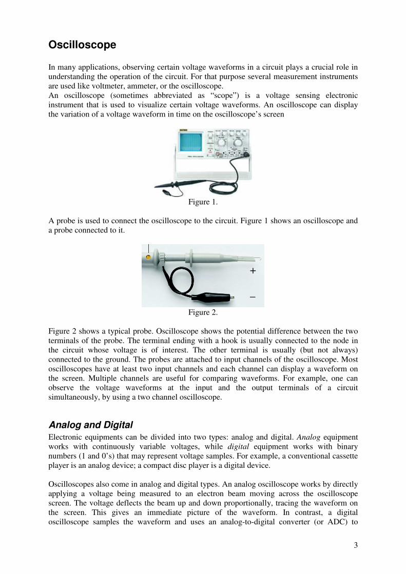
A probe is used to connect the oscilloscope to the circuit. Figure 1 shows an oscilloscope and
a probe connected to it.
Figure 2.
Figure 2 shows a typical probe. Oscilloscope shows the potential difference between the two
terminals of the probe. The terminal ending with a hook is usually connected to the node in
the circuit whose voltage is of interest. The other terminal is usually (but not always)
connected to the ground. The probes are attached to input channels of the oscilloscope. Most
oscilloscopes have at least two input channels and each channel can display a waveform on
the screen. Multiple channels are useful for comparing waveforms. For example, one can
observe the voltage waveforms at the input and the output terminals of a circuit
simultaneously, by using a two channel oscilloscope.
Analog and Digital
Electronic equipments can be divided into two types: analog and digital. Analog equipment
works with continuously variable voltages, while digital equipment works with binary
numbers (1 and 0’s) that may represent voltage samples. For example, a conventional cassette
player is an analog device; a compact disc player is a digital device.
Oscilloscopes also come in analog and digital types. An analog oscilloscope works by directly
applying a voltage being measured to an electron beam moving across the oscilloscope
screen. The voltage deflects the beam up and down proportionally, tracing the waveform on
the screen. This gives an immediate picture of the waveform. In contrast, a digital
oscilloscope samples the waveform and uses an analog-to-digital converter (or ADC) to
+
_

4
convert the voltage being measured into digital information. It then uses this digital
information to reconstruct the waveform on the screen.
Figure 3: Digital and Analog Oscilloscopes Display Waveforms.
Analog Oscilloscopes
An analog oscilloscope displays the voltage waveforms by deflecting an electron beam
generated by an electron gun inside a cathode-ray tube on to a fluorescent coating. Because of
the use of the cathode ray tube, analog oscilloscopes are also known as cathode ray
oscilloscopes. To understand how an analog scope displays the voltage waveforms, it is
necessary to understand what is inside the unit. The following section describes the general
principles of the operation of cathode ray oscilloscopes.

5
Cathode Ray Oscilloscope Principles
Figure 4 shows the structure, and the main components of a cathode ray tube (CRT). Figure 5
shows the face plane of the CRO screen.
Electron Beam
Fluorescent Coating
CRO Screen
Vertical DeflectionPlates
Horizontal DeflectionPlates
Electron Gun
CRO ScreenVertical
DeflectionPlates
Horizontal Deflection
Plates
CRO ScreenVertical
DeflectionPlates
Horizontal Deflection
Plates
Figure 4. Figure 5.
Electron beam generated by the electron gun first deflected by the deflection plates, and then
directed onto the fluorescent coating of the CRO screen, which produces a visible light spot
on the face plane of the oscilloscope screen.
A detailed representation of a CRT is given in Figure 6. The CRT is composed of two main
parts,
• Electron Gun
• Deflection System
Electron Beam
Fluorescent
Coating
Screen
Cathode
Electron Gun
e-
e-
e-
Brightness control
+400V2kV-10kV
-Vgrid
Focus Adjust
Control grid Focus anodes and
electrostatic field
Vertical DeflectionPlates
Horizontal
Deflection
Plates
Deflection System
Figure 6.
Electron Gun
Electron gun provides a sharply focused electron beam directed toward the fluorescent-coated
screen. The thermally heated cathode emits electrons in many directions. The control grid
provides an axial direction for the electron beam and controls the number and speed of
electrons in the beam.
The momentum of the electrons determines the intensity, or brightness, of the light emitted
from the fluorescent coating due to the electron bombardment. Because electrons are

6
negatively charged, a repulsion force is created by applying a negative voltage to the control
grid, to adjust their number and speed. A more negative voltage results in less number of
electrons in the beam and hence decreased brightness of the beam spot.
Since the electron beam consists of many electrons, the beam tends to diverge. This is
because the similar (negative) charges on the electrons repulse each other. To compensate for
such repulsion forces, an adjustable electrostatic field is created between two cylindrical
anodes, called the focusing anodes. The variable positive voltage on the second anode
cylinder is therefore used to adjust the focus or sharpness of the bright spot.
The Deflection System
The deflection system consists of two pairs of parallel plates, referred to as the vertical and
horizontal deflection plates. One of the plates in each set is permanently connected to the
ground (zero volt), whereas the other plate of each set is connected to input signals or
triggering signal of the CRO.
Electron Beam
Fluorescent
Coating
CRO Screen
Vertical Deflection
Plates
Horizontal Deflection
Plates
Electron Gun
Deflection System
Figure 7.
As shown in Figure 7, the electron beam passes through the deflection plates. In reference to
the schematic diagram in Figure 8, a positive voltage applied to the Y input terminal causes
the electron beam to deflect vertically upward, due to attraction forces, while a negative
voltage applied to the Y input terminal causes the electron beam to deflect vertically
downward, due to repulsion forces. Similarly, a positive voltage applied to the X input
terminal will cause the electron beam to deflect horizontally toward the right, while a negative
voltage applied to the X input terminal will cause the electron beam to deflect horizontally
toward the left of the screen.

7
CRO Screen
Vertical Deflection
Plates
Horizontal Deflection
Plates
Vy
Vx
Figure 8.
The amount of vertical or horizontal deflection is directly proportional to the corresponding
applied voltage. When the electrons hit the screen, the phosphor emits light and a visible light
spot is seen on the screen.
Since the amount of deflection is proportional to the applied voltage, actually the voltages Vy
and Vx determine the coordinates of the bright spot created by the electron beam.
Example 1:
Suppose Vx = sin(t), Vy = cos(t) are applied to the horizontal and vertical deflection plates
respectively. Then the bright spot would follow a circular path on the CRO screen.
Vy = cos(t)
Vx = sin(t)
CRO Screen
Figure 9.
8
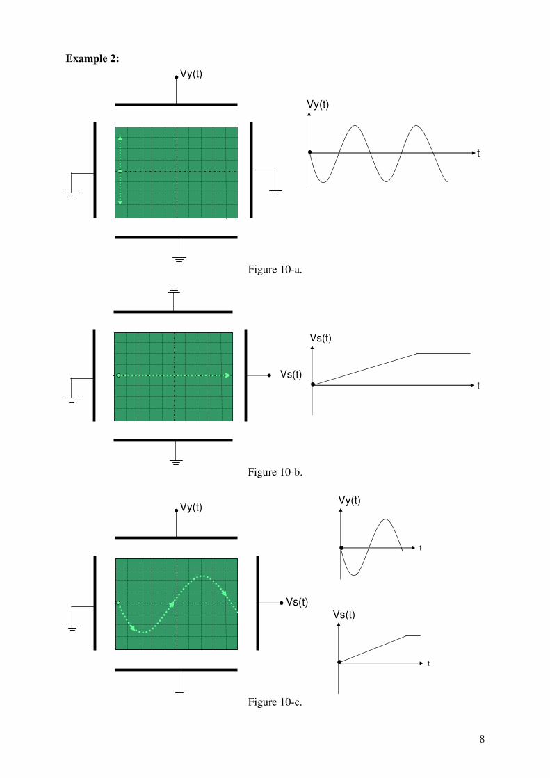
Example 2:
Vy(t)
Vy(t)
t
Figure 10-a.
Vs(t)
Vs(t)
t
Figure 10-b.
Vy(t)Vy(t)
t
Vs(t)
t
Vs(t)
Figure 10-c.
9
In Figure 10-a, the input signal Vy(t) is applied to the vertical deflection plates, whereas the
horizontal deflection plates are connected to ground. It is assumed that the electron beam is
kept at the extreme left position when the horizontal deflection plates are connected to
ground. Under this configuration, the bright spot in the CRO screen will follow a vertical path
(will go up and down) at the extreme left position of the screen.
In Figure 10-b, the input signal Vs(t) is applied to the horizontal deflection plates, whereas the
vertical deflection plates are connected to ground. This time, the bright spot will travel from
extreme left to extreme right end of the screen and will stop there.
In Figure 10-c, the signals Vy(t) and Vs(t) are applied to the vertical and the horizontal
deflection plates respectively. This time the bright spot will follow a sinusoidal path, resulting
a visualization of the input signal Vy(t) on the CRO screen.
Actually the bright spot must follow the same path fast and repetitively (at least 30 times in a
second) so that the human eye can perceive the motion of the bright spot as a continuous
curve. Therefore, in order to display the waveform on the CRO screen for the example in
figure 10-c, the signals Vy(t) and Vs(t) should be applied to the vertical and the horizontal
deflection plates periodically and in synchronization. The next section discusses the details of
this procedure and depicts how CRO handles this problem.
Displaying a Voltage Waveform
In numerous applications it will be required to display a periodical voltage waveform as a
function of time. By applying the voltage to be displayed on the CRO, to the vertical
deflection plates (Vy), the vertical deflection of the beam spot will be proportional to the
magnitude of this voltage. It is then necessary to convert the x axis (horizontal deflection) into
a time axis. Notice that, in the example given in figure 10-c, the voltage waveform Vs(t)
(which varies linearly in time before the bright spot reaches the extreme right end of the
screen) is used for this purpose and the bright spot have traveled the path determined by Vy(t).
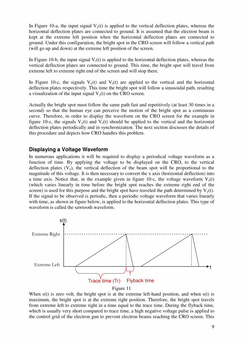
If the signal to be observed is periodic, then a periodic voltage waveform that varies linearly
with time, as shown in figure below, is applied to the horizontal deflection plates. This type of
waveform is called the sawtooth waveform.
t
s(t)
Trace time (Tr)
Extreme Right
Extreme Left
Flyback time
Figure 11
When s(t) is zero volt, the bright spot is at the extreme left-hand position, and when s(t) is
maximum, the bright spot is at the extreme right position. Therefore, the bright spot travels
from extreme left to extreme right in a time equal to the trace time. During the flyback time,
which is usually very short compared to trace time, a high negative voltage pulse is applied to
the control grid of the electron gun to prevent electron beams reaching the CRO screen. This
10
action is called blanking and prevents any reverse retrace (or shadow) as the beam is going
back to the extreme left-hand position. The time period including the trace time and the
flyback time is called the sweep period.
The period of the sawtooth waveform plays a crucial role in obtaining a steady waveform on
the CRO screen. The following section discusses the requirements on the period of the
sawtooth waveform and the need of a synchronization between the sawtooth waveform and
the input waveform.
Triggering
s(t)
t
Vy (t)
t
CRO SCREEN
Steady Waveform is obtained
Extreme Right
Extreme Left
τ
T
Figure 12
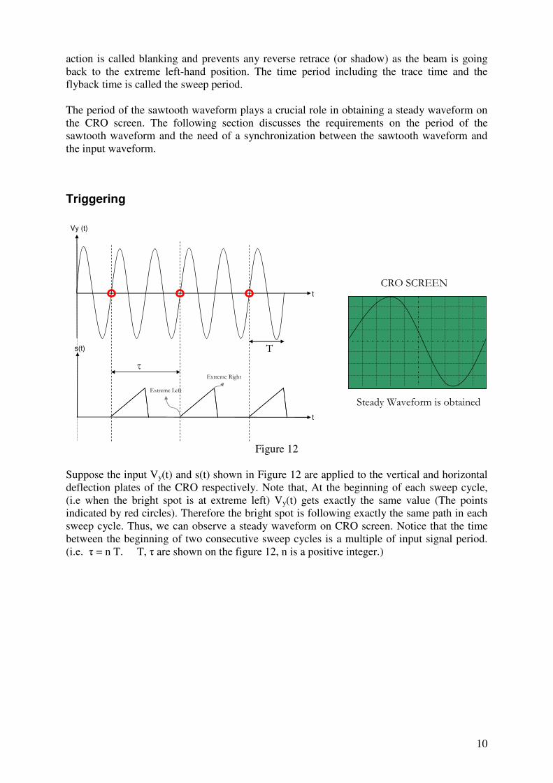
Suppose the input Vy(t) and s(t) shown in Figure 12 are applied to the vertical and horizontal
deflection plates of the CRO respectively. Note that, At the beginning of each sweep cycle,
(i.e when the bright spot is at extreme left) Vy(t) gets exactly the same value (The points
indicated by red circles). Therefore the bright spot is following exactly the same path in each
sweep cycle. Thus, we can observe a steady waveform on CRO screen. Notice that the time
between the beginning of two consecutive sweep cycles is a multiple of input signal period.
(i.e. = n T. T, are shown on the figure 12, n is a positive integer.)
11
S(t)
t
Yinput (t)
t
CRO SCREEN
Waveform is not steady!Extreme Left
Extreme Right
Extreme Left Extreme Left
Extreme Right Extreme Right
Figure 12
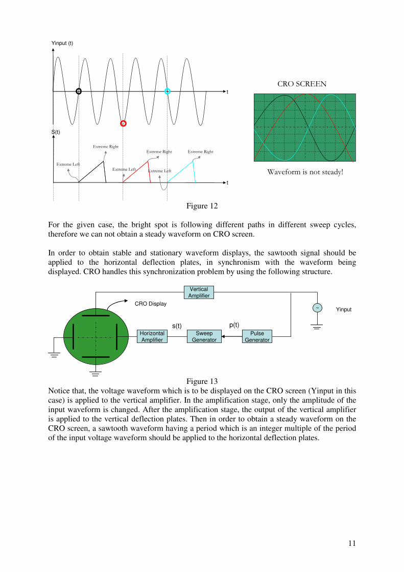
For the given case, the bright spot is following different paths in different sweep cycles,
therefore we can not obtain a steady waveform on CRO screen.
In order to obtain stable and stationary waveform displays, the sawtooth signal should be
applied to the horizontal deflection plates, in synchronism with the waveform being
displayed. CRO handles this synchronization problem by using the following structure.
Yinput
PulseGenerator
~CRO Display
p(t)s(t)HorizontalAmplifier
VerticalAmplifier
SweepGenerator
Figure 13
Notice that, the voltage waveform which is to be displayed on the CRO screen (Yinput in this
case) is applied to the vertical amplifier. In the amplification stage, only the amplitude of the
input waveform is changed. After the amplification stage, the output of the vertical amplifier
is applied to the vertical deflection plates. Then in order to obtain a steady waveform on the
CRO screen, a sawtooth waveform having a period which is an integer multiple of the period
of the input voltage waveform should be applied to the horizontal deflection plates.
12
Yinput (t)
t
Level
t
P(t)
t
S(t)
Trace time (Tr)
T
T
Yinput (t)
t
Level
t
P(t)
t
S(t)
Trace time (Tr)
T
T
Figure 14
Pulse Generator:
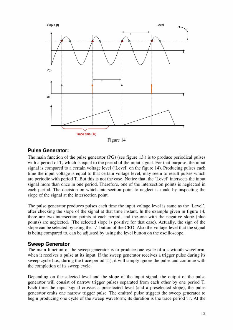
The main function of the pulse generator (PG) (see figure 13.) is to produce periodical pulses
with a period of T, which is equal to the period of the input signal. For that purpose, the input
signal is compared to a certain voltage level (‘Level’ on the figure 14). Producing pulses each
time the input voltage is equal to that certain voltage level, may seem to result pulses which
are periodic with period T. But this is not the case. Notice that, the ‘Level’ intersects the input
signal more than once in one period. Therefore, one of the intersection points is neglected in
each period. The decision on which intersection point to neglect is made by inspecting the
slope of the signal at the intersection point.
The pulse generator produces pulses each time the input voltage level is same as the ‘Level’,
after checking the slope of the signal at that time instant. In the example given in figure 14,
there are two intersection points at each period, and the one with the negative slope (blue
points) are neglected. (The selected slope is positive for that case). Actually, the sign of the
slope can be selected by using the +/- button of the CRO. Also the voltage level that the signal
is being compared to, can be adjusted by using the level button on the oscilloscope.
Sweep Generator The main function of the sweep generator is to produce one cycle of a sawtooth waveform,
when it receives a pulse at its input. If the sweep generator receives a trigger pulse during its
sweep cycle (i.e., during the trace period Tr), it will simply ignore the pulse and continue with
the completion of its sweep cycle.
Depending on the selected level and the slope of the input signal, the output of the pulse
generator will consist of narrow trigger pulses separated from each other by one period T.
Each time the input signal crosses a preselected level (and a preselected slope), the pulse
generator emits one narrow trigger pulse. The emitted pulse triggers the sweep generator to
begin producing one cycle of the sweep waveform; its duration is the trace period Tr. At the
13
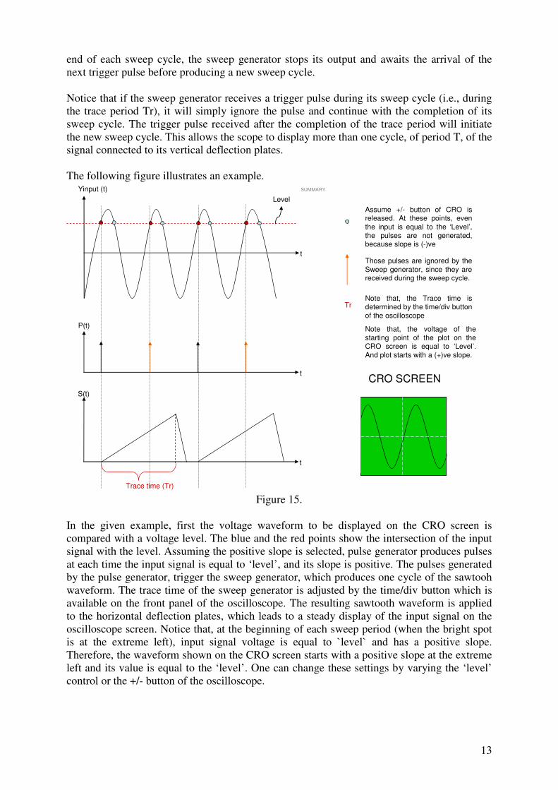
end of each sweep cycle, the sweep generator stops its output and awaits the arrival of the
next trigger pulse before producing a new sweep cycle.
Notice that if the sweep generator receives a trigger pulse during its sweep cycle (i.e., during
the trace period Tr), it will simply ignore the pulse and continue with the completion of its
sweep cycle. The trigger pulse received after the completion of the trace period will initiate
the new sweep cycle. This allows the scope to display more than one cycle, of period T, of the
signal connected to its vertical deflection plates.
The following figure illustrates an example. SUMMARYYinput (t)
t
Level
t
P(t)
t
S(t)
Assume +/- button of CRO is released. At these points, even
the input is equal to the ‘Level’,
the pulses are not generated, because slope is (-)ve
Those pulses are ignored by the
Sweep generator, since they are received during the sweep cycle.
Trace time (Tr)
Note that, the Trace time is determined by the time/div button
of the oscilloscope
Tr
CRO SCREEN
Note that, the voltage of the
starting point of the plot on the CRO screen is equal to ‘Level’.
And plot starts with a (+)ve slope.
Figure 15.
In the given example, first the voltage waveform to be displayed on the CRO screen is
compared with a voltage level. The blue and the red points show the intersection of the input
signal with the level. Assuming the positive slope is selected, pulse generator produces pulses
at each time the input signal is equal to ‘level’, and its slope is positive. The pulses generated
by the pulse generator, trigger the sweep generator, which produces one cycle of the sawtooh
waveform. The trace time of the sweep generator is adjusted by the time/div button which is
available on the front panel of the oscilloscope. The resulting sawtooth waveform is applied
to the horizontal deflection plates, which leads to a steady display of the input signal on the
oscilloscope screen. Notice that, at the beginning of each sweep period (when the bright spot
is at the extreme left), input signal voltage is equal to `level` and has a positive slope.
Therefore, the waveform shown on the CRO screen starts with a positive slope at the extreme
left and its value is equal to the ‘level’. One can change these settings by varying the ‘level’
control or the +/- button of the oscilloscope.
14
The whole process is called triggering because, obtaining a steady plot on the CRO screen can
only be achieved by producing pulses at the input of the Sweep Generator at the correct time
instances. (i.e. triggering the Sweep Generator at the correct time instances.)
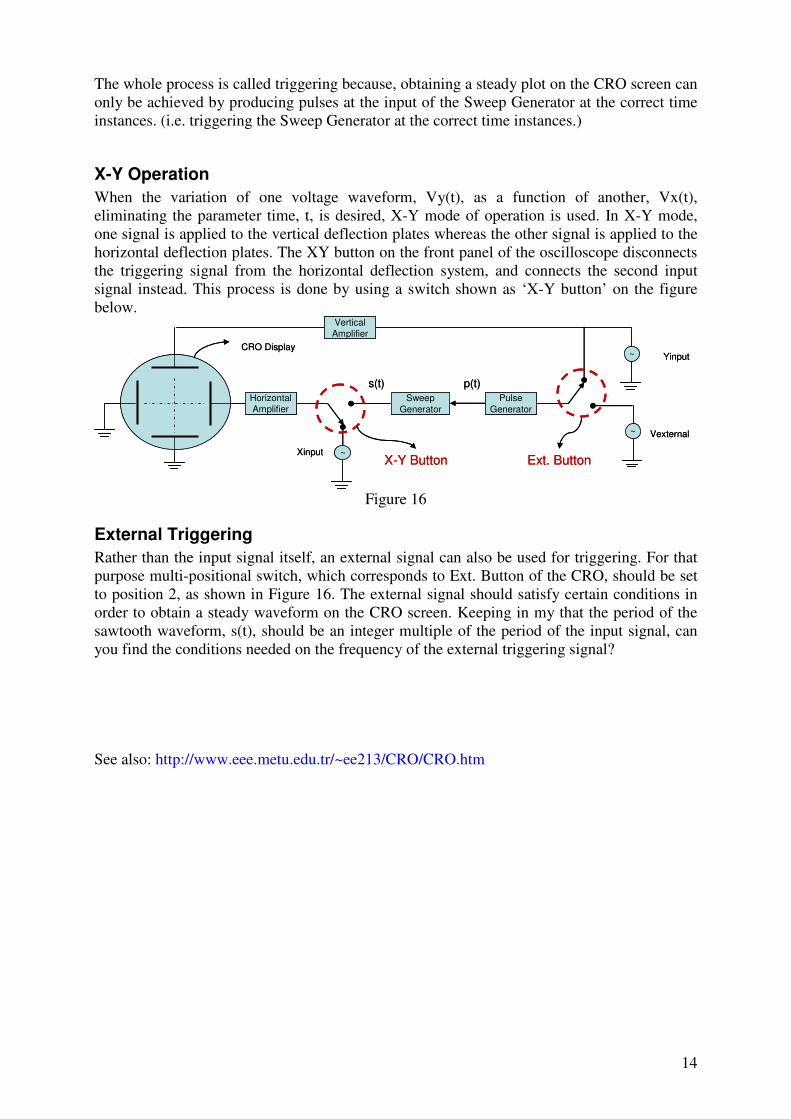
X-Y Operation
When the variation of one voltage waveform, Vy(t), as a function of another, Vx(t),
eliminating the parameter time, t, is desired, X-Y mode of operation is used. In X-Y mode,
one signal is applied to the vertical deflection plates whereas the other signal is applied to the
horizontal deflection plates. The XY button on the front panel of the oscilloscope disconnects
the triggering signal from the horizontal deflection system, and connects the second input
signal instead. This process is done by using a switch shown as ‘X-Y button’ on the figure
below.
Yinput
Sweep
Generator
Pulse
Generator
~ Vexternal
~CRO Display
p(t)s(t)
Horizontal
Amplifier
Vertical
Amplifier
Xinput ~X-Y Button Ext. Button
Yinput
Sweep
Generator
Pulse
Generator
~ Vexternal
~CRO Display
p(t)s(t)
Horizontal
Amplifier
Vertical
Amplifier
Xinput ~X-Y Button Ext. Button
Figure 16
External Triggering
Rather than the input signal itself, an external signal can also be used for triggering. For that
purpose multi-positional switch, which corresponds to Ext. Button of the CRO, should be set
to position 2, as shown in Figure 16. The external signal should satisfy certain conditions in
order to obtain a steady waveform on the CRO screen. Keeping in my that the period of the
sawtooth waveform, s(t), should be an integer multiple of the period of the input signal, can
you find the conditions needed on the frequency of the external triggering signal?
See also: http://www.eee.metu.edu.tr/~ee213/CRO/CRO.htm
15
Digital Storage Oscilloscopes (DSO)
The concept behind the digital oscilloscope is somewhat different to an analogue scope.
Rather than processing the signals in an analogue fashion, the DSO converts them into a
digital format using an analogue to digital converter (ADC), then it stores the digital data in
the memory, and then processes the signals digitally, finally it converts the resulting signal in
a picture format to be displayed on the screen of the scope.
Since the waveform is stored in a digital format, the data can be processed either within the
oscilloscope itself, or even by a PC connected to it. One advantage of using the DSO is that
the stored data can be used to visualize or process the signal at any time. The analogue scopes
do not have memory therefore the signal can be displayed only instantaneously. The transient
parts of the signal (which may vanish even in milliseconds or microseconds) can not be
observed using an analogue oscilloscope.
The DSO’s are widely used in many applications in view of their flexibility and performance.
16
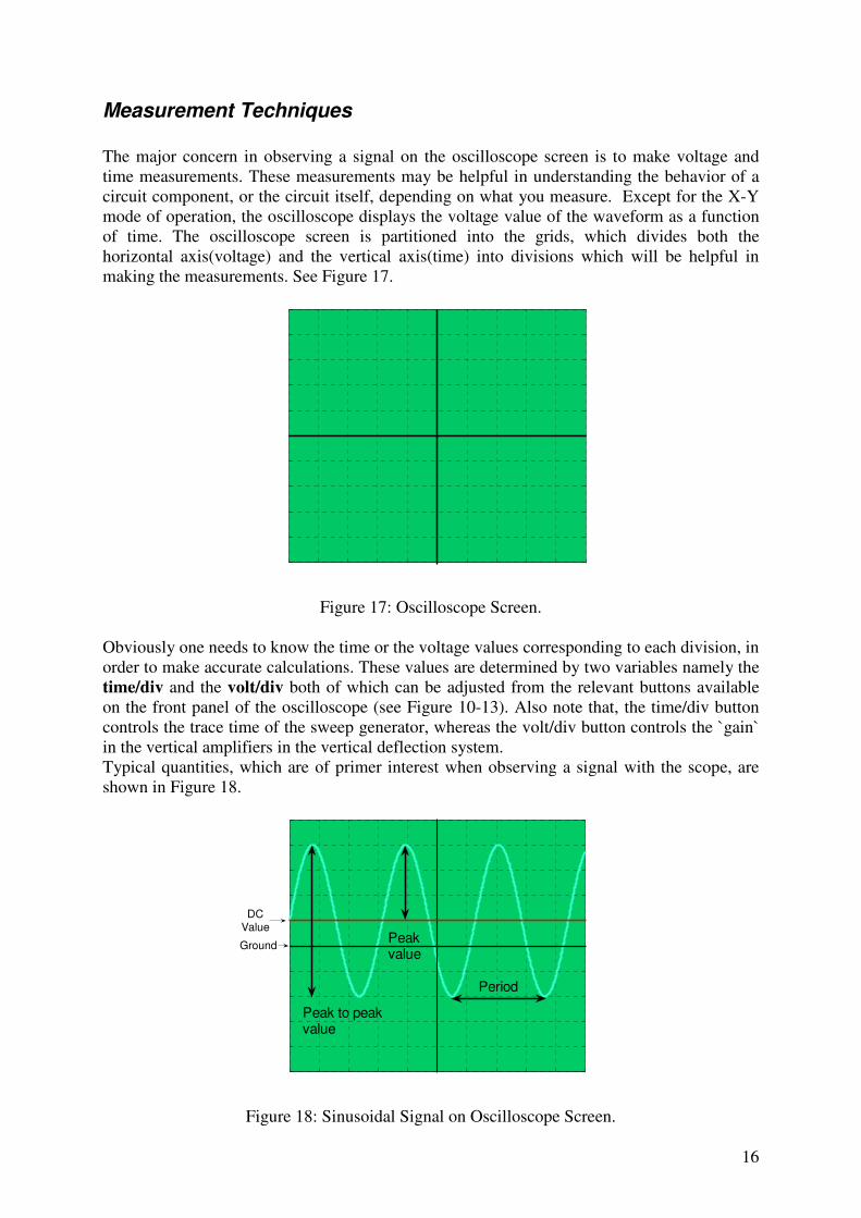
Measurement Techniques
The major concern in observing a signal on the oscilloscope screen is to make voltage and
time measurements. These measurements may be helpful in understanding the behavior of a
circuit component, or the circuit itself, depending on what you measure. Except for the X-Y
mode of operation, the oscilloscope displays the voltage value of the waveform as a function
of time. The oscilloscope screen is partitioned into the grids, which divides both the
horizontal axis(voltage) and the vertical axis(time) into divisions which will be helpful in
making the measurements. See Figure 17.
0 0 . 1 0 . 2 0 . 3 0 . 4 0 . 5 0 . 6 0 . 7 0 . 8 0 . 9 1
- 5
- 4
- 3
- 2
- 1
0
1
2
3
4
5
Figure 17: Oscilloscope Screen.
Obviously one needs to know the time or the voltage values corresponding to each division, in
order to make accurate calculations. These values are determined by two variables namely the
time/div and the volt/div both of which can be adjusted from the relevant buttons available
on the front panel of the oscilloscope (see Figure 10-13). Also note that, the time/div button
controls the trace time of the sweep generator, whereas the volt/div button controls the `gain`
in the vertical amplifiers in the vertical deflection system.
Typical quantities, which are of primer interest when observing a signal with the scope, are
shown in Figure 18.
0 2 4 6 8 1 0 1 2 1 4 1 6 1 8 2 0
- 5
- 4
- 3
- 2
- 1
0
1
2
3
4
5
DCValue
Ground
Period
Peak to peakvalue
Peakvalue
Figure 18: Sinusoidal Signal on Oscilloscope Screen.
17
For the given figure, suppose that the variables volt/div and time/div are set to:
volt/div = 2Volts/div.
time/div = 1millisecond/div
Then the corresponding values shown on the figure are calculated to be;
Peak Value = 6volts
Peak to peak value = 12 Volts
DC Value (Average Value) = 2 Volts
Period = 3 milliseconds
Frequency = =Period
1333 Hz.
Note that the signal s(t), shown on the oscilloscope screen can be expressed as,
( )( )( )
sin(2 )
6sin 2 333 2
6sin 666 2 .
peak DCs t V ft V
t
t Volts
π
ππ
= +
= +
= +
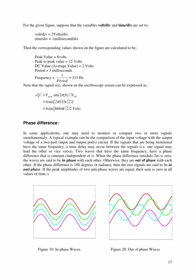
Phase difference:
In some applications, one may need to monitor or compare two or more signals
simultaneously. A typical example can be the comparison of the input voltage with the output
voltage of a two-port (input and output ports) circuit. If the signals that are being monitored
have the same frequency, a time delay may occur between the signals (i.e. one signal may
lead the other or vice versa). Two waves that have the same frequency, have a phase
difference that is constant (independent of t). When the phase difference (modulo 2 ) is zero,
the waves are said to be in phase with each other. Otherwise, they are out of phase with each
other. If the phase difference is 180 degrees ( radians), then the two signals are said to be in
anti-phase. If the peak amplitudes of two anti-phase waves are equal, their sum is zero at all
values of time, t.
0 2 4 6 8 1 0 1 2 1 4 1 6 1 8 2 0
- 5
- 4
- 3
- 2
- 1
0
1
2
3
4
5
0 2 4 6 8 1 0 1 2 1 4 1 6 1 8 2 0
- 5
- 4
- 3
- 2
- 1
0
1
2
3
4
5
Figure 19: In-phase Waves Figure 20: Out of phase Waves
18
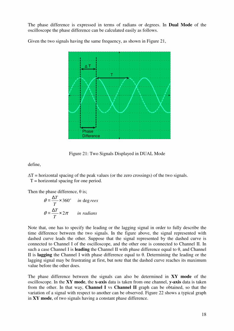
The phase difference is expressed in terms of radians or degrees. In Dual Mode of the
oscilloscope the phase difference can be calculated easily as follows.
Given the two signals having the same frequency, as shown in Figure 21,
0 2 4 6 8 1 0 1 2 1 4 1 6 1 8 2 0
- 5
- 4
- 3
- 2
- 1
0
1
2
3
4
5
PhaseDifference
∆ T
T
Figure 21: Two Signals Displayed in DUAL Mode
define,
T = horizontal spacing of the peak values (or the zero crossings) of the two signals.
T = horizontal spacing for one period.
Then the phase difference, is;
radiansinT
T
reesinT
T o
πθ
θ
2
deg360
×∆=
×∆=
Note that, one has to specify the leading or the lagging signal in order to fully describe the
time difference between the two signals. In the figure above, the signal represented with
dashed curve leads the other. Suppose that the signal represented by the dashed curve is
connected to Channel I of the oscilloscope, and the other one is connected to Channel II. In
such a case Channel I is leading the Channel II with phase difference equal to , and Channel
II is lagging the Channel I with phase difference equal to . Determining the leading or the
lagging signal may be frustrating at first, but note that the dashed curve reaches its maximum
value before the other does.
The phase difference between the signals can also be determined in XY mode of the
oscilloscope. In the XY mode, the x-axis data is taken from one channel, y-axis data is taken
from the other. In that way, Channel I vs Channel II graph can be obtained, so that the
variation of a signal with respect to another can be observed. Figure 22 shows a typical graph
in XY mode, of two signals having a constant phase difference.

19
- 5 - 4 - 3 - 2 - 1 0 1 2 3 4 5
- 5
- 4
- 3
- 2
- 1
0
1
2
3
4
5
Figure 22: Phase Difference Calculation in XY Mode
Phase difference is equal to,
1sinA
Bθ − =
.
One can show this relation by expressing one signal as, )sin(2
)( θ±= wtB
ty and the other
signal as, ( ) sin( )2
Cx t wt= . Then consider the value of y(t) when x(t) is zero volts. It should be
noted that, the center of the ellipsoidal shape (sometimes circular or linear shapes) on the
screen should be at the origin of CRO unless any DC component is added to one of the
signals.
In XY mode, the leading or the lagging signal can not be determined. One has to switch to
DUAL mode in order to specify the leading signal.
Figure 23 shows typical graphs in XY mode corresponding to different values of phase
difference.
- 5 - 4 - 3 - 2 - 1 0 1 2 3 4 5
- 5
- 4
- 3
- 2
- 1
0
1
2
3
4
5
- 5 - 4 - 3 - 2 - 1 0 1 2 3 4 5
- 5
- 4
- 3
- 2
- 1
0
1
2
3
4
5
- 5 - 4 - 3 - 2 - 1 0 1 2 3 4 5
- 5
- 4
- 3
- 2
- 1
0
1
2
3
4
5
- 5 - 4 - 3 - 2 - 1 0 1 2 3 4 5
- 5
- 4
- 3
- 2
- 1
0
1
2
3
4
5
0° 45° 90° 180°
Figure 23: The Graphs in XY Mode for Different Phase Difference Values
B A
20
Controls
Display Controls
Display systems may vary between analog and digital oscilloscopes. Common controls
include:
• An intensity control to adjust the brightness of the waveform. As you increase the
sweep speed of an analog oscilloscope, you need to increase the intensity level.
• A focus control to adjust the sharpness of the waveform. Digital oscilloscopes may not
have a focus control.
• Other display controls may let you adjust the intensity of lights and turn on or off any
on-screen information (such as menus).
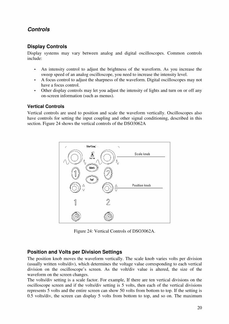
Vertical Controls
Vertical controls are used to position and scale the waveform vertically. Oscilloscopes also
have controls for setting the input coupling and other signal conditioning, described in this
section. Figure 24 shows the vertical controls of the DSO3062A
Figure 24: Vertical Controls of DSO3062A.
Position and Volts per Division Settings
The position knob moves the waveform vertically. The scale knob varies volts per division
(usually written volts/div), which determines the voltage value corresponding to each vertical
division on the oscilloscope’s screen. As the volt/div value is altered, the size of the
waveform on the screen changes.
The volts/div setting is a scale factor. For example, If there are ten vertical divisions on the
oscilloscope screen and if the volts/div setting is 5 volts, then each of the vertical divisions
represents 5 volts and the entire screen can show 50 volts from bottom to top. If the setting is
0.5 volts/div, the screen can display 5 volts from bottom to top, and so on. The maximum

21
voltage you can display on the screen is the volts/div setting times the number of vertical
divisions.
Often the volts/div scale has either a variable gain or a fine gain control for scaling a
displayed signal to a certain number of divisions. Figure 25 shows the vertical controls of the
HM203-7 CRO.
Figure 25: Vertical Controls of HM203-7 CRO
Horizontal Controls
Horizontal controls are used to position and scale the waveform horizontally. Figure 26 and
27 show typical front panel for the horizontal controls.
Figure 26: Horizontal Controls of
DSO3062A
Figure 27: Horizontal Controls of HM203-7
CRO
The horizontal position control (x-pos.) is used to move the waveform from left and right to
exactly where you want it on the screen.
The time per division (time/div) setting lets you select the rate at which the waveform is
drawn across the screen (also known as the time base setting or sweep speed). This setting is a
scale factor. For example, if the setting is 1 ms, each horizontal division represents 1 ms and
the total screen width represents 10 ms (ten divisions). Changing the time/div setting lets you
look at longer or shorter time intervals of the input signal.
As with the vertical volts/div scale, the horizontal sec/div scale may have variable timing,
allowing you to set the horizontal time scale in between the discrete settings.
Also note that, the time/div button actually controls the trace time of sawtooth waveform in
the sweep generator. When sawtooth waveform is zero volt, the bright spot is at the extreme
left-hand position, and when it is maximum, the bright spot is at the extreme right position.
Therefore, the bright spot travels from extreme left to extreme right in a time equal to the
Trace time. Assume that the CRO screen is divided into N equal horizontal divisions. The
bright spot travels the N divisions in Tr seconds. Therefore each division corresponds to
22
(Tr/N) seconds. If the Trace time is changed, the corresponding time for each division is
changed. Time per division controls can be used to select the appropriate time/div (i.e., the
Trace time of the sawtooth waveform).
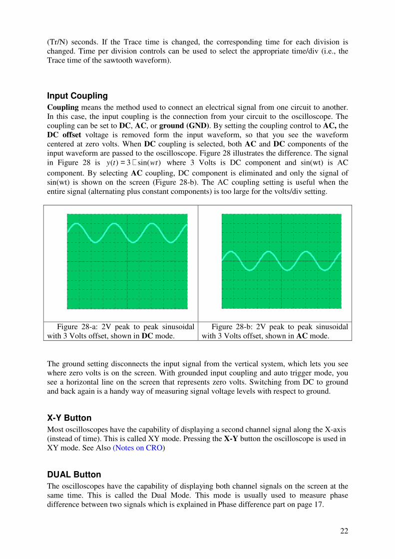
Input Coupling
Coupling means the method used to connect an electrical signal from one circuit to another.
In this case, the input coupling is the connection from your circuit to the oscilloscope. The
coupling can be set to DC, AC, or ground (GND). By setting the coupling control to AC, the
DC offset voltage is removed form the input waveform, so that you see the waveform
centered at zero volts. When DC coupling is selected, both AC and DC components of the
input waveform are passed to the oscilloscope. Figure 28 illustrates the difference. The signal
in Figure 28 is )sin(3)( wtty += where 3 Volts is DC component and sin(wt) is AC
component. By selecting AC coupling, DC component is eliminated and only the signal of
sin(wt) is shown on the screen (Figure 28-b). The AC coupling setting is useful when the
entire signal (alternating plus constant components) is too large for the volts/div setting.
0 2 4 6 8 1 0 1 2 1 4 1 6 1 8 2 0
- 5
- 4
- 3
- 2
- 1
0
1
2
3
4
5
0 2 4 6 8 1 0 1 2 1 4 1 6 1 8 2 0
- 5
- 4
- 3
- 2
- 1
0
1
2
3
4
5
Figure 28-a: 2V peak to peak sinusoidal
with 3 Volts offset, shown in DC mode.
Figure 28-b: 2V peak to peak sinusoidal
with 3 Volts offset, shown in AC mode.
The ground setting disconnects the input signal from the vertical system, which lets you see
where zero volts is on the screen. With grounded input coupling and auto trigger mode, you
see a horizontal line on the screen that represents zero volts. Switching from DC to ground
and back again is a handy way of measuring signal voltage levels with respect to ground.
X-Y Button
Most oscilloscopes have the capability of displaying a second channel signal along the X-axis
(instead of time). This is called XY mode. Pressing the X-Y button the oscilloscope is used in
XY mode. See Also (Notes on CRO)
DUAL Button
The oscilloscopes have the capability of displaying both channel signals on the screen at the
same time. This is called the Dual Mode. This mode is usually used to measure phase
difference between two signals which is explained in Phase difference part on page 17.
23
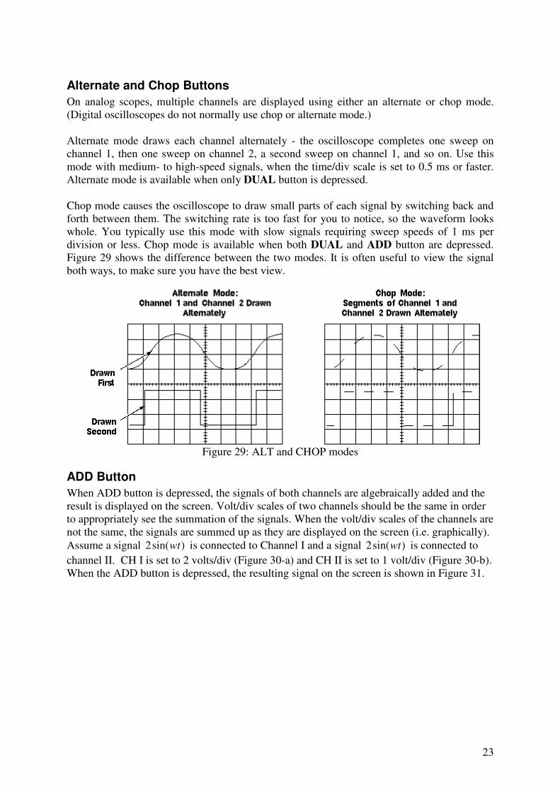
Alternate and Chop Buttons
On analog scopes, multiple channels are displayed using either an alternate or chop mode.
(Digital oscilloscopes do not normally use chop or alternate mode.)
Alternate mode draws each channel alternately - the oscilloscope completes one sweep on
channel 1, then one sweep on channel 2, a second sweep on channel 1, and so on. Use this
mode with medium- to high-speed signals, when the time/div scale is set to 0.5 ms or faster.
Alternate mode is available when only DUAL button is depressed.
Chop mode causes the oscilloscope to draw small parts of each signal by switching back and
forth between them. The switching rate is too fast for you to notice, so the waveform looks
whole. You typically use this mode with slow signals requiring sweep speeds of 1 ms per
division or less. Chop mode is available when both DUAL and ADD button are depressed.
Figure 29 shows the difference between the two modes. It is often useful to view the signal
both ways, to make sure you have the best view.
Figure 29: ALT and CHOP modes
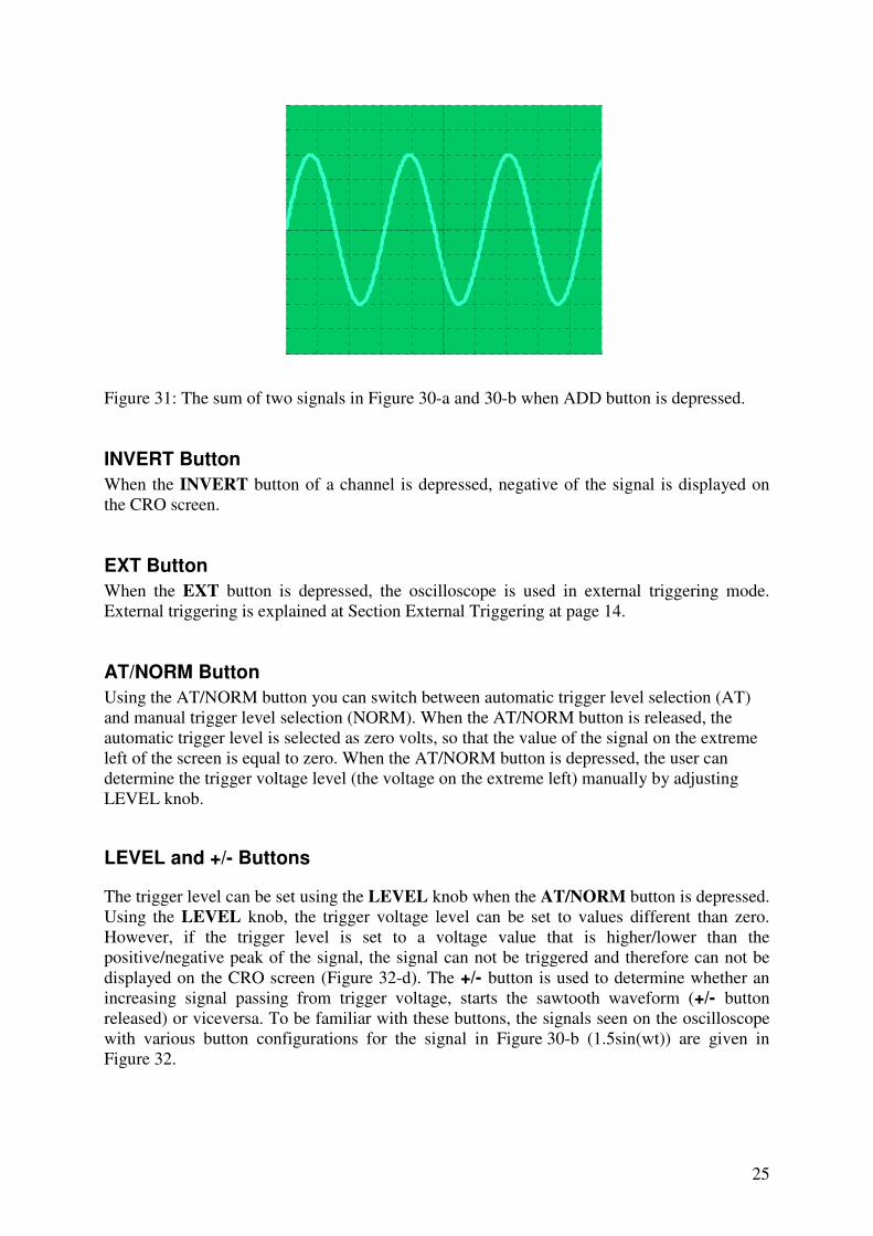
ADD Button
When ADD button is depressed, the signals of both channels are algebraically added and the
result is displayed on the screen. Volt/div scales of two channels should be the same in order
to appropriately see the summation of the signals. When the volt/div scales of the channels are
not the same, the signals are summed up as they are displayed on the screen (i.e. graphically).
Assume a signal )sin(2 wt is connected to Channel I and a signal )sin(2 wt is connected to
channel II. CH I is set to 2 volts/div (Figure 30-a) and CH II is set to 1 volt/div (Figure 30-b).
When the ADD button is depressed, the resulting signal on the screen is shown in Figure 31.

24
0 2 4 6 8 1 0 1 2 1 4 1 6 1 8 2 0
- 5
- 4
- 3
- 2
- 1
0
1
2
3
4
5
0 2 4 6 8 1 0 1 2 1 4 1 6 1 8 2 0
- 5
- 4
- 3
- 2
- 1
0
1
2
3
4
5
Figure 30-a: The first signal seen on the
oscilloscope with 2 volt/div scale.
Figure 30-b: The second signal seen on the
oscilloscope with 1 volt/div scale.
25
0 2 4 6 8 1 0 1 2 1 4 1 6 1 8 2 0
- 5
- 4
- 3
- 2
- 1
0
1
2
3
4
5
Figure 31: The sum of two signals in Figure 30-a and 30-b when ADD button is depressed.
INVERT Button
When the INVERT button of a channel is depressed, negative of the signal is displayed on
the CRO screen.
EXT Button
When the EXT button is depressed, the oscilloscope is used in external triggering mode.
External triggering is explained at Section External Triggering at page 14.
AT/NORM Button
Using the AT/NORM button you can switch between automatic trigger level selection (AT)
and manual trigger level selection (NORM). When the AT/NORM button is released, the
automatic trigger level is selected as zero volts, so that the value of the signal on the extreme
left of the screen is equal to zero. When the AT/NORM button is depressed, the user can
determine the trigger voltage level (the voltage on the extreme left) manually by adjusting
LEVEL knob.
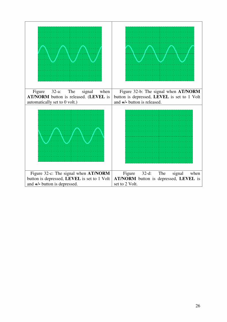
LEVEL and +/- Buttons
The trigger level can be set using the LEVEL knob when the AT/NORM button is depressed.
Using the LEVEL knob, the trigger voltage level can be set to values different than zero.
However, if the trigger level is set to a voltage value that is higher/lower than the
positive/negative peak of the signal, the signal can not be triggered and therefore can not be
displayed on the CRO screen (Figure 32-d). The +/- button is used to determine whether an
increasing signal passing from trigger voltage, starts the sawtooth waveform (+/- button
released) or viceversa. To be familiar with these buttons, the signals seen on the oscilloscope
with various button configurations for the signal in Figure 30-b (1.5sin(wt)) are given in
Figure 32.
26
0 2 4 6 8 1 0 1 2 1 4 1 6 1 8 2 0
- 5
- 4
- 3
- 2
- 1
0
1
2
3
4
5
0 2 4 6 8 1 0 1 2 1 4 1 6 1 8 2 0
- 5
- 4
- 3
- 2
- 1
0
1
2
3
4
5
Figure 32-a: The signal when
AT/NORM button is released. (LEVEL is
automatically set to 0 volt.)
Figure 32-b: The signal when AT/NORM
button is depressed, LEVEL is set to 1 Volt
and +/- button is released.
0 2 4 6 8 1 0 1 2 1 4 1 6 1 8 2 0
- 5
- 4
- 3
- 2
- 1
0
1
2
3
4
5
0 2 4 6 8 1 0 1 2 1 4 1 6 1 8 2 0
- 5
- 4
- 3
- 2
- 1
0
1
2
3
4
5
Figure 32-c: The signal when AT/NORM
button is depressed, LEVEL is set to 1 Volt
and +/- button is depressed.
Figure 32-d: The signal when
AT/NORM button is depressed, LEVEL is
set to 2 Volt.
27
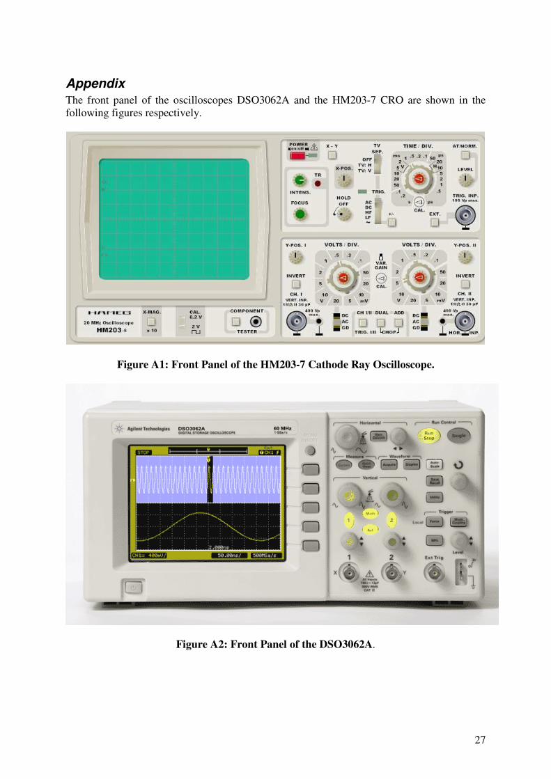
Appendix
The front panel of the oscilloscopes DSO3062A and the HM203-7 CRO are shown in the
following figures respectively.
Figure A1: Front Panel of the HM203-7 Cathode Ray Oscilloscope.
Figure A2: Front Panel of the DSO3062A.

28
Figure A3: Schematic for the Front Panel of the DSO3062A.


