Nucleation rates of ethanol Nucleation rates of ethanol and methanol using an and methanol using an equation of state.equation of state.

Noura Al-Zoubi Noura Al-Zoubi

Advisor:Advisor:

Dr. Abdalla ObeidatDr. Abdalla Obeidat

Co-advisor:Co-advisor:

Dr. Maen GharaibehDr. Maen Gharaibeh

Out LinesOut Lines::

• Introduction.Introduction.

• First order phase transition.First order phase transition.

• Classical nucleation theory Classical nucleation theory (CNT).(CNT).

• Gradient theory (GT).Gradient theory (GT).

• Computational methodology.Computational methodology.

• Results and conclusion.Results and conclusion.

DefinitionDefinition

• Nucleation is the process which the formation Nucleation is the process which the formation of new phases begins and is thus a widely of new phases begins and is thus a widely spread phenomenon in both nature and spread phenomenon in both nature and technology.technology.

• Nucleation refers to the kinetic processes Nucleation refers to the kinetic processes involved in the initiation of the first order phase involved in the initiation of the first order phase transition in non equilibrium systems.transition in non equilibrium systems.

• Condensation and evaporation, crystal Condensation and evaporation, crystal growth, deposition of thin films and overall growth, deposition of thin films and overall crystallization are only a few of the processes crystallization are only a few of the processes in which nucleation plays a prominent role. in which nucleation plays a prominent role.

..

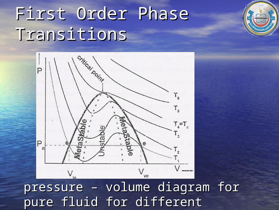
First Order Phase TransitionsFirst Order Phase Transitions

pressure – volume diagram for pure pressure – volume diagram for pure fluid for different isotherms.fluid for different isotherms.

dependence of the reduced pressure dependence of the reduced pressure and Gibbs energy on the reduced and Gibbs energy on the reduced volume using VDWvolume using VDW

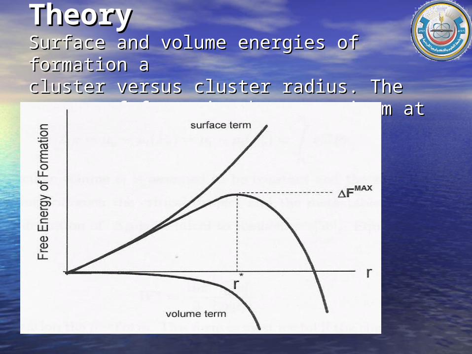
Classical Nucleation Classical Nucleation TheoryTheory Surface and volume energies of formation a Surface and volume energies of formation a cluster versus cluster radius. The energy of cluster versus cluster radius. The energy of formation has a maximum at critical radius.formation has a maximum at critical radius.

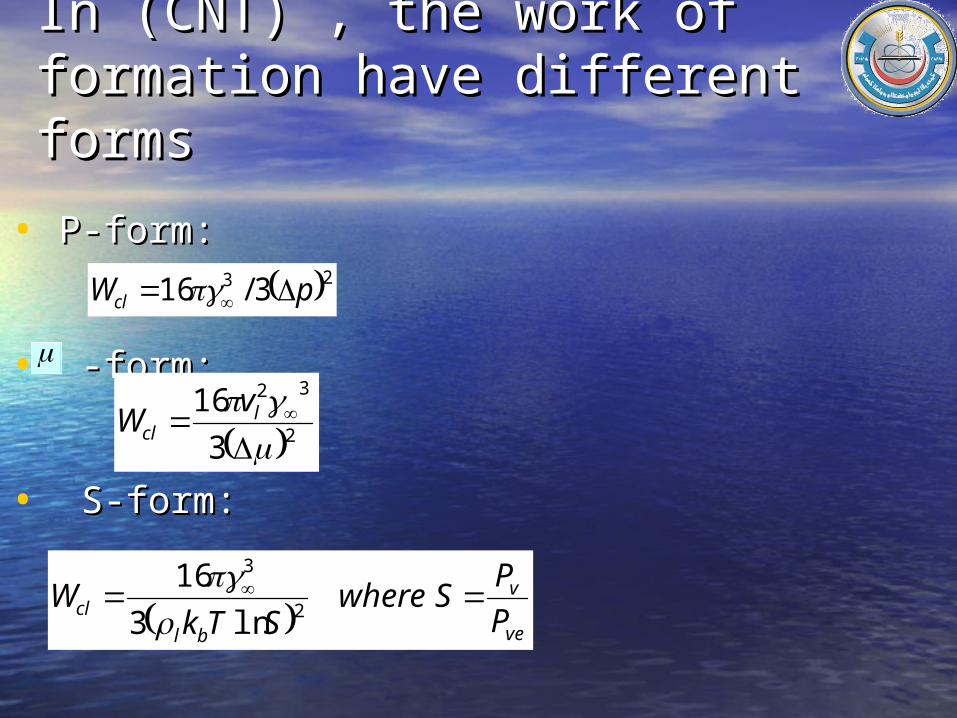
In (CNT) , the work of In (CNT) , the work of formation have different formsformation have different forms

• P-form: P-form:

• -form:-form:

• S-form:S-form:

23 3/16 pWcl

2

32

3

16

l

cl

vW

ve

v

bl

cl P

PSwhere

STkW

2

3

ln3

16

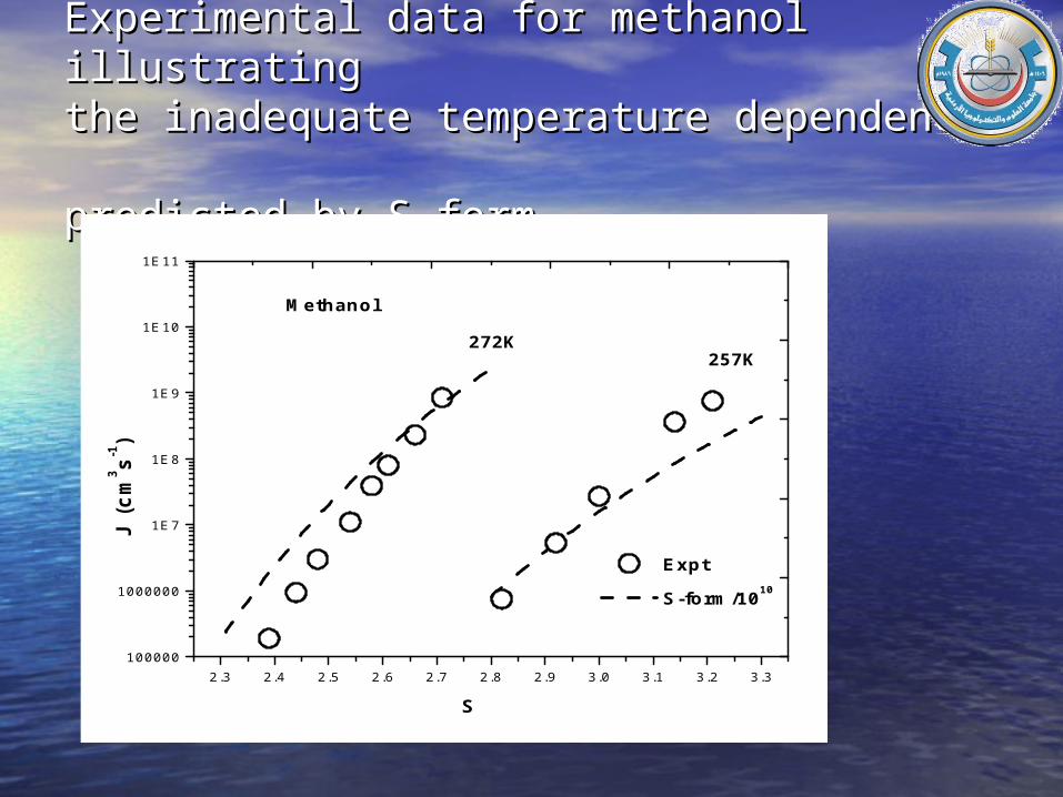
Experimental data for methanol illustratingExperimental data for methanol illustratingthe inadequate temperature dependence the inadequate temperature dependence predicted by S-form.predicted by S-form.

2.3 2.4 2.5 2.6 2.7 2.8 2.9 3.0 3.1 3.2 3.3100000

1000000

1E7

1E8

1E9

1E10

1E11

272K

Expt

S-form/1010

Methanol

257K

J (

cm

3 s-1)

S

Experimental data for ethanol illustrating the Experimental data for ethanol illustrating the inadequate temperature dependence inadequate temperature dependence predicted by S-form.predicted by S-form.

2.5 3.0100000

1E8

1E11

Ethanol

expt

S-form/107

J (c

m-3s-1

)

S

286K293K

Density functional theory Density functional theory and the road to gradient and the road to gradient theorytheoryDFTDFT AdvantagesAdvantages• Powerful technique Powerful technique that has been used to that has been used to

explore varies systems.explore varies systems.

DisadvantagesDisadvantages

• Require exact Require exact intermolecular intermolecular

Potential. Potential.

GTGT AdvantagesAdvantages• Requires a Cubic Requires a Cubic

EOSEOSDisadvantagesDisadvantages

• An approximation An approximation to DFTto DFT

• The Helmholtz free energy density is The Helmholtz free energy density is given as:given as:

• The density profile can be determined by The density profile can be determined by integrating the following equation:integrating the following equation:

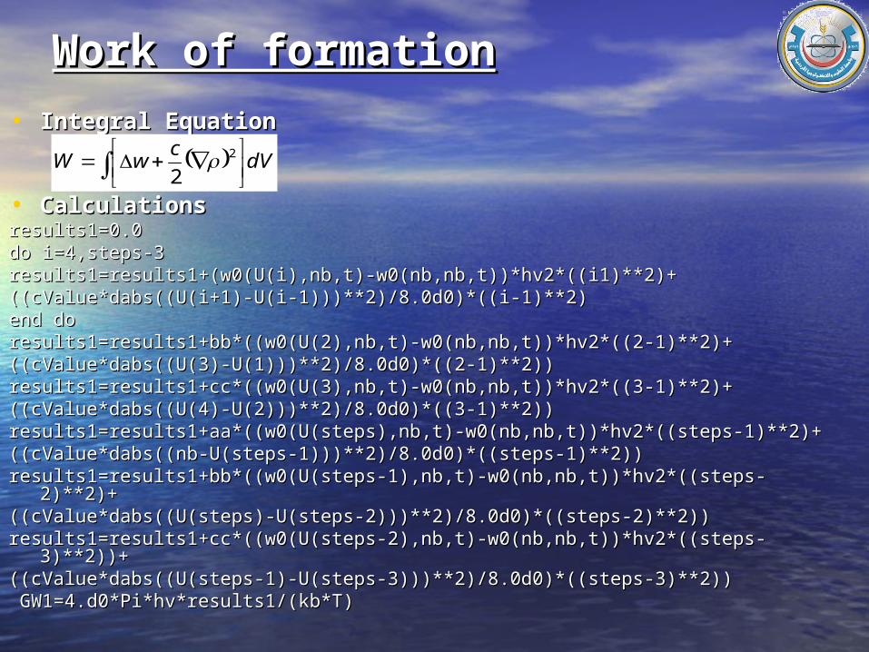
• The work of formation is given as:The work of formation is given as:

Gradient Gradient TheoryTheory

20 2

c

ff

0

2

)()()(

2

fwandwwwwhere

dVc

wW

b

02

2 12

cdr

d

rdr

d

Experimental nucleation rates of Experimental nucleation rates of methanol compared to the predictionsmethanol compared to the predictionsof GT with the CPHB EOS.of GT with the CPHB EOS.

2.2 2.4 2.6 2.8 3.0 3.210

5

106

107

108

109

JGT

/107

Jexp

Methanol

T=272 KT=257 K

J (

cm-3s-1

)

S

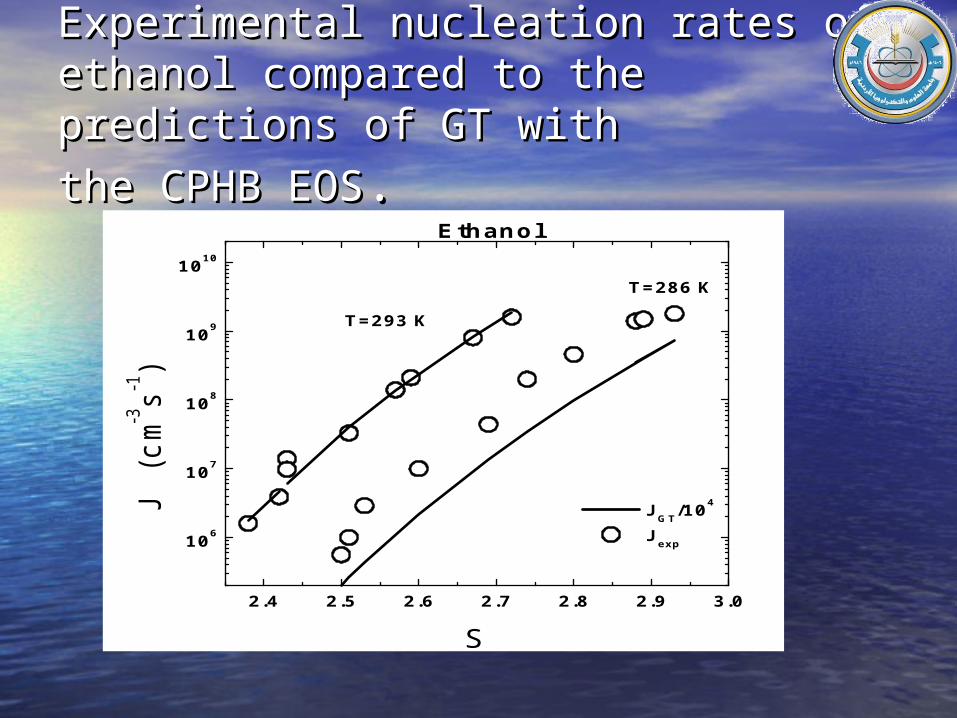
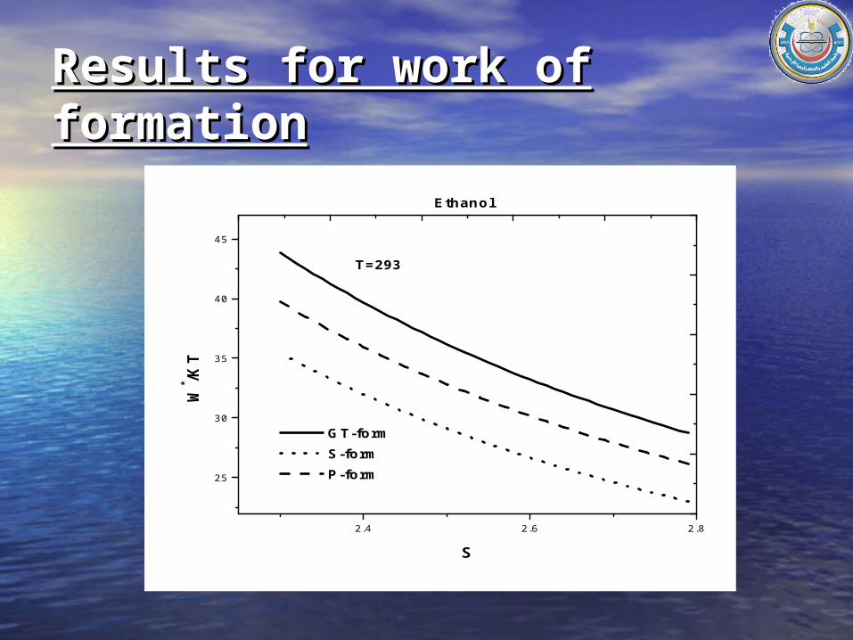
Experimental nucleation rates of Experimental nucleation rates of ethanol compared to the predictions of ethanol compared to the predictions of GT with GT with

the CPHB EOSthe CPHB EOS..

2.4 2.5 2.6 2.7 2.8 2.9 3.0

106

107

108

109

1010

JGT/104

Jexp

Ethanol

T=286 K

T=293 K

J

(cm-3

s-1)

S

SAFT-EOSSAFT-EOS• Exact EOS for low TExact EOS for low T

• Cubic EOSCubic EOS

Computational Computational MethodologyMethodology• Equilibrium Densities of liquid and vaporEquilibrium Densities of liquid and vapor

1. Conditions1. Conditions

2. Calculations using Newton-Raphson method2. Calculations using Newton-Raphson method dodo row(1)=guess1row(1)=guess1 row(2)=guess2row(2)=guess2 k(1,1)=dp(row(1),t)k(1,1)=dp(row(1),t) k(1,2)=-dp(row(2),t)k(1,2)=-dp(row(2),t) k(2,1)=dmew(row(1),t)k(2,1)=dmew(row(1),t) k(2,2)=-dmew(row(2),t)k(2,2)=-dmew(row(2),t) f(1)=p(row(2),t)-p(row(1),t) f(1)=p(row(2),t)-p(row(1),t) f(2)=mew(row(2),t)-mew(row(1),t)f(2)=mew(row(2),t)-mew(row(1),t) z=k(2,1)/k(1,1)z=k(2,1)/k(1,1) k(2,1)=0.0d0k(2,1)=0.0d0 f(2)=f(2)-(z*f(1))f(2)=f(2)-(z*f(1)) k(2,2)=k(2,2)-(z*k(1,2))k(2,2)=k(2,2)-(z*k(1,2)) u(2)=f(2)/k(2,2)u(2)=f(2)/k(2,2) u(1)=(f(1)-k(1,2)*u(2))/k(1,1)u(1)=(f(1)-k(1,2)*u(2))/k(1,1) row=row+urow=row+u end doend do

Influence ParameterInfluence Parameter

• Experimental surface tensionExperimental surface tension Surface=(23.88-0.08807*(T-273))*10-7Surface=(23.88-0.08807*(T-273))*10-7• GT surface tension

• Equivalence between GT and experimental surface Equivalence between GT and experimental surface tensionstensions

C=C=(Surface/integral)2 /2(Surface/integral)2 /2 where C: influence parameter where C: influence parameterIntegral=

• Calculations using Composite Simpson method Calculations using Composite Simpson method step=4001step=4001h1=(row(1)-row(2))/steph1=(row(1)-row(2))/step sum=0.d0sum=0.d0sum1=0.d0sum1=0.d0do i=1,(step/2.d0)-1do i=1,(step/2.d0)-1x1=row(2)+2.d0*i*h1x1=row(2)+2.d0*i*h1x2=row(2)+(2.d0*i-1)*h1x2=row(2)+(2.d0*i-1)*h1sum=sum+(2.d0*h1/3.d0)*deltaW(x1,row(2),t)sum=sum+(2.d0*h1/3.d0)*deltaW(x1,row(2),t)sum1=sum1+(4.d0*h1/3.d0)*deltaW(x2,row(2),t)sum1=sum1+(4.d0*h1/3.d0)*deltaW(x2,row(2),t)end doend dointegral=(h1/3.d0)*(deltaW(row(2),row(2),t)+deltaW(row(1),row(2),t))+integral=(h1/3.d0)*(deltaW(row(2),row(2),t)+deltaW(row(1),row(2),t))+sum+sum1sum+sum1

dwwcle

ve

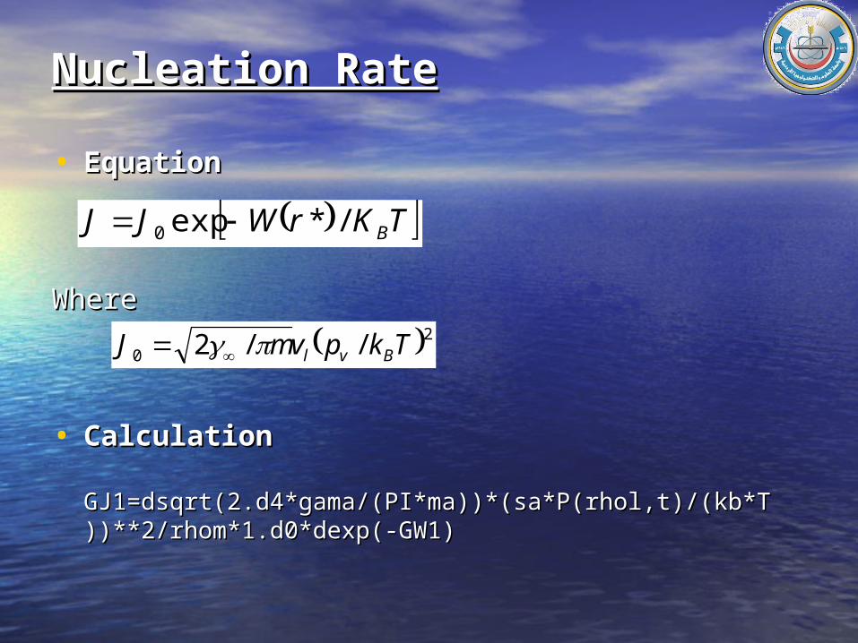
p

p

ve 2

dwwle

ve

ve ))()((

Droplet Density Profile Droplet Density Profile

• Second order differential EquationSecond order differential Equation

wherewhere

• Boundary conditionsBoundary conditions

as and asas and as

02

22 12

Cdr

d

rdr

dC

0dr

d 0r b r

hdr

dand

hdr

d iiiii

2

2 112

112

2

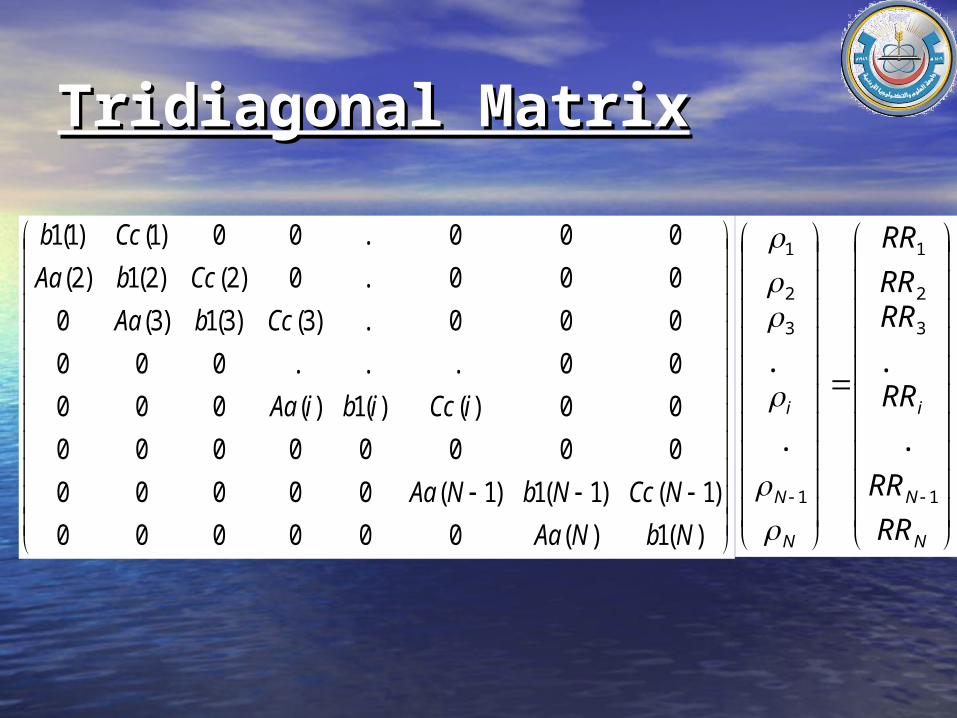
Tridiagonal MatrixTridiagonal Matrix

)(1)(000000

)1()1(1)1(00000

00000000

00)()(1)(000

00...000

000.)3()3(1)3(0

000.0)2()2(1)2(

000.00)1()1(1

NbNAa

NCcNbNAa

iCcibiAa

CcbAa

CcbAa

Ccb

N

N

i

N

N

i

RR

RR

RR

RRRR

RR

1

3

2

1

1

3

2

1

.

.

.

.

Tridiagonal MatrixTridiagonal Matrix

• Construction of tridiagonal matrixConstruction of tridiagonal matrixdo do do i=2,stepsdo i=2,stepsAa(i)=i-2Aa(i)=i-2 B1(i)=-1*(i-1)*(2.d0+hv2*dmew(U(i),t)/CValue)B1(i)=-1*(i-1)*(2.d0+hv2*dmew(U(i),t)/CValue)Cc(i)=iCc(i)=iRR(i)=(i-1)*hv2*Gg(U(i),nb,t)/CValueRR(i)=(i-1)*hv2*Gg(U(i),nb,t)/CValueend doend doAa(1)=0Aa(1)=0B1(1)=-(6.d0+hv2*dmew(U(1),t)/CValue)B1(1)=-(6.d0+hv2*dmew(U(1),t)/CValue)Cc(1)=6.d0Cc(1)=6.d0Cc(steps)=0Cc(steps)=0RR(1)=hv2*Gg(U(1),nb,t)/CValueRR(1)=hv2*Gg(U(1),nb,t)/CValueRR(steps)=(steps-1)*hv2*Gg(U(steps),nb,t)/CValue-(steps)*nbRR(steps)=(steps-1)*hv2*Gg(U(steps),nb,t)/CValue-(steps)*nb

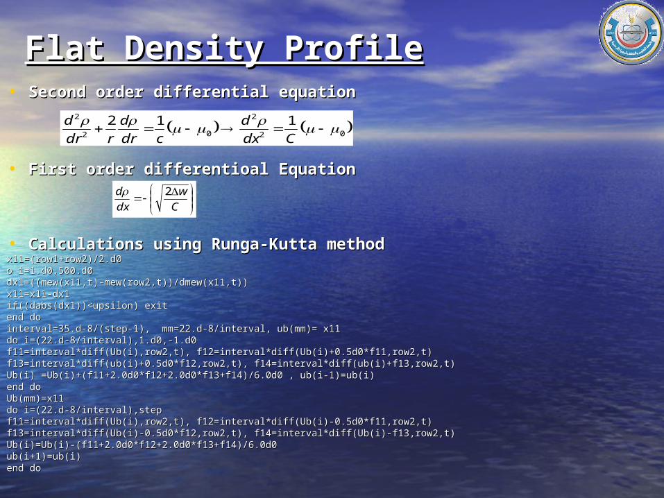
Flat Density ProfileFlat Density Profile• Second order differential equationSecond order differential equation

• First order differentioal EquationFirst order differentioal Equation

• Calculations using Runga-Kutta methodCalculations using Runga-Kutta methodx11=(row1+row2)/2.d0x11=(row1+row2)/2.d0o i=1.d0,500.d0o i=1.d0,500.d0dx1=((mew(x11,t)-mew(row2,t))/dmew(x11,t))dx1=((mew(x11,t)-mew(row2,t))/dmew(x11,t))x11=x11-dx1x11=x11-dx1if((dabs(dx1))<upsilon) exitif((dabs(dx1))<upsilon) exitend doend dointerval=35.d-8/(step-1), mm=22.d-8/interval, ub(mm)= x11interval=35.d-8/(step-1), mm=22.d-8/interval, ub(mm)= x11do i=(22.d-8/interval),1.d0,-1.d0do i=(22.d-8/interval),1.d0,-1.d0f11=interval*diff(Ub(i),row2,t), f12=interval*diff(Ub(i)+0.5d0*f11,row2,t)f11=interval*diff(Ub(i),row2,t), f12=interval*diff(Ub(i)+0.5d0*f11,row2,t)f13=interval*diff(ub(i)+0.5d0*f12,row2,t), f14=interval*diff(ub(i)+f13,row2,t)f13=interval*diff(ub(i)+0.5d0*f12,row2,t), f14=interval*diff(ub(i)+f13,row2,t)Ub(i) =Ub(i)+(f11+2.0d0*f12+2.0d0*f13+f14)/6.0d0 , ub(i-1)=ub(i)Ub(i) =Ub(i)+(f11+2.0d0*f12+2.0d0*f13+f14)/6.0d0 , ub(i-1)=ub(i)end doend doUb(mm)=x11Ub(mm)=x11do i=(22.d-8/interval),stepdo i=(22.d-8/interval),stepf11=interval*diff(Ub(i),row2,t), f12=interval*diff(Ub(i)-0.5d0*f11,row2,t) f11=interval*diff(Ub(i),row2,t), f12=interval*diff(Ub(i)-0.5d0*f11,row2,t) f13=interval*diff(Ub(i)-0.5d0*f12,row2,t), f14=interval*diff(Ub(i)-f13,row2,t)f13=interval*diff(Ub(i)-0.5d0*f12,row2,t), f14=interval*diff(Ub(i)-f13,row2,t)Ub(i)=Ub(i)-(f11+2.0d0*f12+2.0d0*f13+f14)/6.0d0 Ub(i)=Ub(i)-(f11+2.0d0*f12+2.0d0*f13+f14)/6.0d0 ub(i+1)=ub(i)ub(i+1)=ub(i)end doend do

C

w

dx

d 2

02

2

02

2 112

Cdx

d

cdr

d

rdr

d

Flat density profileFlat density profile

0 1 2 3 4

0.000

0.005

0.010

0.015

(m

ol/c

m3 )

r(nm)

Tridiagonal MatrixTridiagonal Matrix

)(1)(000000

)1()1(1)1(00000

00000000

00)()(1)(000

00...000

000.)3()3(1)3(0

000.0)2()2(1)2(

000.00)1()1(1

NbNAa

NCcNbNAa

iCcibiAa

CcbAa

CcbAa

Ccb

N

N

i

N

N

i

RR

RR

RR

RRRR

RR

1

3

2

1

1

3

2

1

.

.

.

.

Solution of Tridiagonal MatrixSolution of Tridiagonal Matrix

• Lower Upper (LU) Decomposition methodLower Upper (LU) Decomposition methodn=stepsn=steps

bet=b1(1)bet=b1(1)

u(1)=rr(1)/betu(1)=rr(1)/bet

do j=2,ndo j=2,n

gam(j)=cc(j-1)/betgam(j)=cc(j-1)/bet

bet=b1(j)-aa(j)*gam(j)bet=b1(j)-aa(j)*gam(j)

u(j)=(rr(j)-aa(j)*u(j-1))/betu(j)=(rr(j)-aa(j)*u(j-1))/bet

end doend do

do j=n-1,1,-1do j=n-1,1,-1

u(j)=u(j)-gam(j+1)*u(j+1)u(j)=u(j)-gam(j+1)*u(j+1)

end do end do

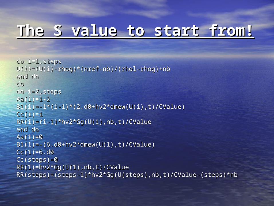
The S value to start from!The S value to start from!

do i=1,stepsdo i=1,stepsU(i)=(U(i)-rhog)*(nref-nb)/(rhol-rhog)+nbU(i)=(U(i)-rhog)*(nref-nb)/(rhol-rhog)+nbend doend dodo do do i=2,stepsdo i=2,stepsAa(i)=i-2Aa(i)=i-2 B1(i)=-1*(i-1)*(2.d0+hv2*dmew(U(i),t)/CValue)B1(i)=-1*(i-1)*(2.d0+hv2*dmew(U(i),t)/CValue)Cc(i)=iCc(i)=iRR(i)=(i-1)*hv2*Gg(U(i),nb,t)/CValueRR(i)=(i-1)*hv2*Gg(U(i),nb,t)/CValueend doend doAa(1)=0Aa(1)=0B1(1)=-(6.d0+hv2*dmew(U(1),t)/CValue)B1(1)=-(6.d0+hv2*dmew(U(1),t)/CValue)Cc(1)=6.d0Cc(1)=6.d0Cc(steps)=0Cc(steps)=0RR(1)=hv2*Gg(U(1),nb,t)/CValueRR(1)=hv2*Gg(U(1),nb,t)/CValueRR(steps)=(steps-1)*hv2*Gg(U(steps),nb,t)/CValue-(steps)*nbRR(steps)=(steps-1)*hv2*Gg(U(steps),nb,t)/CValue-(steps)*nb

Comparison between flat density Comparison between flat density profile and density profile at profile and density profile at S=1.65S=1.65

0 1 2 3 4

0.000

0.005

0.010

0.015

Flat Density profile density profile at S=1.65

(m

ol/c

m3 )

r(nm)

11

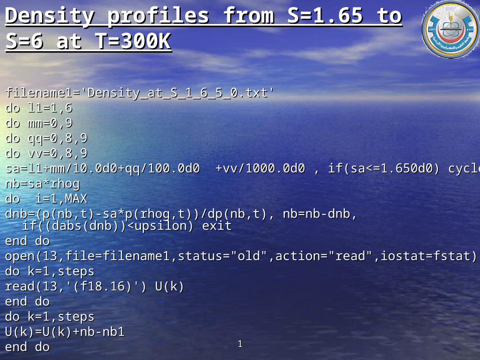
Density profiles from S=1.65 to S=6 Density profiles from S=1.65 to S=6 at T=300Kat T=300K

filename1='Density_at_S_1_6_5_0.txt'filename1='Density_at_S_1_6_5_0.txt'do l1=1,6do l1=1,6do mm=0,9do mm=0,9do qq=0,8,9do qq=0,8,9do vv=0,8,9do vv=0,8,9sa=l1+mm/10.0d0+qq/100.0d0 +vv/1000.0d0 , if(sa<=1.650d0) cyclesa=l1+mm/10.0d0+qq/100.0d0 +vv/1000.0d0 , if(sa<=1.650d0) cyclenb=sa*rhognb=sa*rhogdo i=1,MAXdo i=1,MAXdnb=(p(nb,t)-sa*p(rhog,t))/dp(nb,t), nb=nb-dnb, if((dabs(dnb))<upsilon) dnb=(p(nb,t)-sa*p(rhog,t))/dp(nb,t), nb=nb-dnb, if((dabs(dnb))<upsilon)

exitexitend doend doopen(13,file=filename1,status="old",action="read",iostat=fstat)open(13,file=filename1,status="old",action="read",iostat=fstat)do k=1,stepsdo k=1,stepsread(13,'(f18.16)') U(k)read(13,'(f18.16)') U(k)end doend dodo k=1,stepsdo k=1,stepsU(k)=U(k)+nb-nb1U(k)=U(k)+nb-nb1end doend do

22

dododo i=1,stepsdo i=1,stepsAa(i)=i-2Aa(i)=i-2 B1(i)=-1.d0*(i-1)*(2.d0+hv2*dmew(U(i),t)/CValue)B1(i)=-1.d0*(i-1)*(2.d0+hv2*dmew(U(i),t)/CValue)Cc(i)=iCc(i)=iRR(i)=(i-1)*hv2*Gg(U(i),nb,t)/CValueRR(i)=(i-1)*hv2*Gg(U(i),nb,t)/CValueend doend doAa(1)=0Aa(1)=0B1(1)=-(6.d0+hv2*dmew(U(1),t)/CValue)B1(1)=-(6.d0+hv2*dmew(U(1),t)/CValue)Cc(1)=6.d0Cc(1)=6.d0Cc(steps)=0Cc(steps)=0RR(1)=hv2*Gg(U(1),nb,t)/CValueRR(1)=hv2*Gg(U(1),nb,t)/CValueRR(steps)=(steps-1)*hv2*Gg(U(steps),nb,t)/CValue-(steps)*nbRR(steps)=(steps-1)*hv2*Gg(U(steps),nb,t)/CValue-(steps)*nbend doend doend do end do end doend doend doend docall tridag_ser(aa,b1,cc,RR,X1,steps)call tridag_ser(aa,b1,cc,RR,X1,steps)error=0.d0 error=0.d0 do i=1,stepsdo i=1,stepserror=error+(X1(i)-U(i))**2error=error+(X1(i)-U(i))**2end doend doerror=sqrt(dabs(error))error=sqrt(dabs(error))U=X1U=X1if (error<Upsilon) exitif (error<Upsilon) exitend doend do

Results for density profiles with Results for density profiles with different supersaturation different supersaturation values.values.

0.0 0.5 1.0 1.5 2.0 2.5 3.0 3.5

0.000

0.005

0.010

0.015

0.020

S=1.65 S=2 S=2.65 S=3 S=3.65

(m

ol/cm3 )

r(nm)

T=300K

11

Density profiles from T=300K to Density profiles from T=300K to T=230K at S=6T=230K at S=6

filename1='Density_at_S_6_0_0_0.filename1='Density_at_S_6_0_0_0.txt'txt'

do T=300.d0,230.d0,-1.d0do T=300.d0,230.d0,-1.d0if(T==300.d0)cycleif(T==300.d0)cycledodorow(1)=guess1row(1)=guess1row(2)=guess2row(2)=guess2k(1,1)=dp(row(1),t)k(1,1)=dp(row(1),t)k(1,2)=-dp(row(2),t)k(1,2)=-dp(row(2),t)k(2,1)=dmew(row(1),t)k(2,1)=dmew(row(1),t)k(2,2)=-dmew(row(2),t)k(2,2)=-dmew(row(2),t)f(1)=p(row(2),t)-p(row(1),t) f(1)=p(row(2),t)-p(row(1),t) f(2)=mew(row(2),t)-mew(row(1),t)f(2)=mew(row(2),t)-mew(row(1),t)z=k(2,1)/k(1,1)z=k(2,1)/k(1,1)k(2,1)=0.0d0k(2,1)=0.0d0f(2)=f(2)-(z*f(1))f(2)=f(2)-(z*f(1))k(2,2)=k(2,2)-(z*k(1,2))k(2,2)=k(2,2)-(z*k(1,2))

u1(2)=f(2)/k(2,2)u1(2)=f(2)/k(2,2) u1(1)=(f(1)-k(1,2)*u1(2))/k(1,1)u1(1)=(f(1)-k(1,2)*u1(2))/k(1,1) row=row+u1row=row+u1 error1=0.0d0error1=0.0d0 do i=1,2do i=1,2 error1=error1+f(i)**2error1=error1+f(i)**2 end doend do error1=dsqrt(error1)error1=dsqrt(error1) if (error1<Upsilon) exitif (error1<Upsilon) exit guess1=row(1)guess1=row(1) guess2=row(2)guess2=row(2) end doend doTs=T-273.15d0Ts=T-273.15d0gama = (23.88d0-.08807d0*Ts)*1.d-7gama = (23.88d0-.08807d0*Ts)*1.d-7row1=row(1)row1=row(1)row2=row(2)row2=row(2)steps=4001steps=4001h1=(row1-row2)/stepsh1=(row1-row2)/steps

22

do k1=1,stepsdo k1=1,stepsread(13,'(f18.16)') U(k1)read(13,'(f18.16)') U(k1)end doend doclose(13)close(13)do k1=1,stepsdo k1=1,stepsU(k1)=U(k1)+nb-nb1U(k1)=U(k1)+nb-nb1end doend docounter=0 counter=0 do sum=0.d0do sum=0.d0sum1=0.d0sum1=0.d0do i=1,(steps/2.d0)-1do i=1,(steps/2.d0)-1x1=row2+2.d0*i*h1x1=row2+2.d0*i*h1x2=row2+(2.d0*i-1)*h1x2=row2+(2.d0*i-1)*h1sum=sum+(2.d0*h1/3.d0)*deltaW(x1sum=sum+(2.d0*h1/3.d0)*deltaW(x1

,row2,t),row2,t)sum1=sum1+(4.d0*h1/3.d0)*deltaW(sum1=sum1+(4.d0*h1/3.d0)*deltaW(

x2,row2,t)x2,row2,t)end doend dointegral=(h1/3.d0)*(deltaW(row2,rowintegral=(h1/3.d0)*(deltaW(row2,row

2,t)+deltaW(row1,row2,t))2,t)+deltaW(row1,row2,t))+sum+sum1+sum+sum1

cvalue=(gama/integral)**2/2.d0cvalue=(gama/integral)**2/2.d0rhog=row(2)rhog=row(2)rhol=row(1)rhol=row(1)sa=6.d0sa=6.d0

nb=sa*rhognb=sa*rhogdo i=1,MAXdo i=1,MAXdnb=(p(nb,t)-sa*p(rhog,t))/dp(nb,t)dnb=(p(nb,t)-sa*p(rhog,t))/dp(nb,t) nb=nb-dnbnb=nb-dnb if((dabs(dnb))<upsilon) exitif((dabs(dnb))<upsilon) exit print*,i,dnbprint*,i,dnb end doend do hv=(35.d-8/(steps-1))hv=(35.d-8/(steps-1)) hv2=hv**2hv2=hv**2nb1=nbnb1=nbopen(13,file=filename1,status="old",actioopen(13,file=filename1,status="old",actio

n="read",iostat=fstatn="read",iostat=fstatread(13,'(I7)') stepsread(13,'(I7)') steps

counter=counter+1counter=counter+1do i=2,stepsdo i=2,stepsAa(i)=i-2Aa(i)=i-2

B1(i)=-1.d0*(i-B1(i)=-1.d0*(i-

1)*(2.d0+hv2*dmew(U(i),t)/CValue)1)*(2.d0+hv2*dmew(U(i),t)/CValue)Cc(i)=iCc(i)=iRR(i)=(i-1)*hv2*Gg(U(i),nb,t)/CValueRR(i)=(i-1)*hv2*Gg(U(i),nb,t)/CValue

33

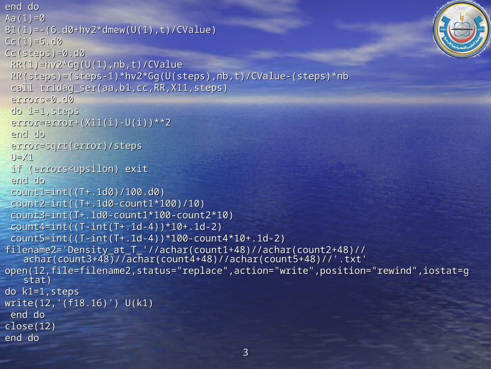
end doend doAa(1)=0Aa(1)=0B1(1)=-(6.d0+hv2*dmew(U(1),t)/CValue)B1(1)=-(6.d0+hv2*dmew(U(1),t)/CValue)Cc(1)=6.d0Cc(1)=6.d0Cc(steps)=0.d0Cc(steps)=0.d0 RR(1)=hv2*Gg(U(1),nb,t)/CValueRR(1)=hv2*Gg(U(1),nb,t)/CValue RR(steps)=(steps-1)*hv2*Gg(U(steps),nb,t)/CValue-(steps)*nbRR(steps)=(steps-1)*hv2*Gg(U(steps),nb,t)/CValue-(steps)*nb call tridag_ser(aa,b1,cc,RR,X11,steps)call tridag_ser(aa,b1,cc,RR,X11,steps) errors=0.d0 errors=0.d0 do i=1,stepsdo i=1,steps error=error+(X11(i)-U(i))**2error=error+(X11(i)-U(i))**2 end doend do error=sqrt(error)/stepserror=sqrt(error)/steps U=X1U=X1 if (errors<upsilon) exitif (errors<upsilon) exit end doend do count1=int((T+.1d0)/100.d0)count1=int((T+.1d0)/100.d0) count2=int((T+.1d0-count1*100)/10)count2=int((T+.1d0-count1*100)/10) count3=int(T+.1d0-count1*100-count2*10)count3=int(T+.1d0-count1*100-count2*10) count4=int((T-int(T+.1d-4))*10+.1d-2)count4=int((T-int(T+.1d-4))*10+.1d-2) count5=int((T-int(T+.1d-4))*100-count4*10+.1d-2)count5=int((T-int(T+.1d-4))*100-count4*10+.1d-2)filename2='Density_at_T_'//achar(count1+48)//achar(count2+48)//achar(count3+48)//filename2='Density_at_T_'//achar(count1+48)//achar(count2+48)//achar(count3+48)//

achar(count4+48)//achar(count5+48)//'.txt' achar(count4+48)//achar(count5+48)//'.txt' open(12,file=filename2,status="replace",action="write",position="rewind",iostat=gstat)open(12,file=filename2,status="replace",action="write",position="rewind",iostat=gstat)do k1=1,stepsdo k1=1,stepswrite(12,'(f18.16)') U(k1)write(12,'(f18.16)') U(k1) end doend doclose(12)close(12)end doend do

Results for density profiles with Results for density profiles with different temperatures.different temperatures.

0.0 0.5 1.0 1.5 2.0 2.5 3.0 3.5

0.000

0.005

0.010

0.015

0.020S=6

T=300 T=290 T=280 T=270

(m

ol/c

m3 )

r(nm)

11

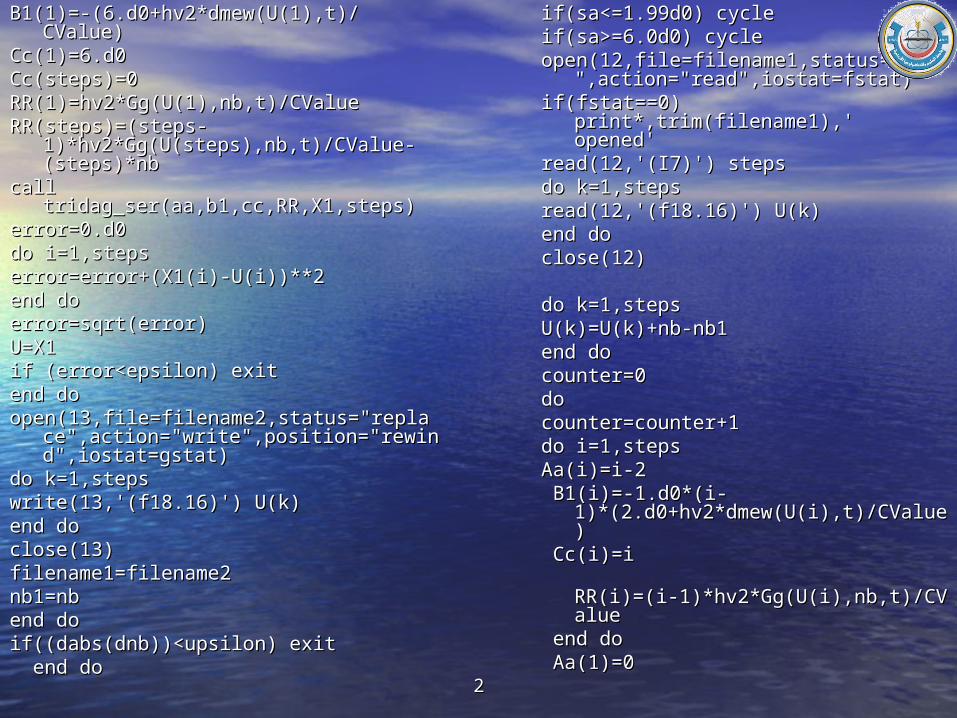
Density profiles from S=6 to S=2 at Density profiles from S=6 to S=2 at T=293KT=293K

T=293.d0T=293.d0Ts=T-273.15d0Ts=T-273.15d0gama = (23.88d0-.08807d0*Ts)*1.d-7gama = (23.88d0-.08807d0*Ts)*1.d-7cvalue=5.974465658636744d-10cvalue=5.974465658636744d-10sa=6.d0 sa=6.d0 rhog=3.656930116927259d-6rhog=3.656930116927259d-6rhol=1.711839175934329d-2rhol=1.711839175934329d-2nb=sa*rhognb=sa*rhogdo i=1,MAXdo i=1,MAXdnb=(p(nb,t)-sa*p(rhog,t))/dp(nb,t)dnb=(p(nb,t)-sa*p(rhog,t))/dp(nb,t)nb=nb-dnbnb=nb-dnbif((dabs(dnb))<upsilon) exitif((dabs(dnb))<upsilon) exitend doend dohv=(35.d-8/(steps-1))hv=(35.d-8/(steps-1))hv2=hv**2hv2=hv**2nb1=nbnb1=nbfilename1='Density_at_T_2_9_3.txt'filename1='Density_at_T_2_9_3.txt'do sa=6.0d0,2.0d0,-.01d0do sa=6.0d0,2.0d0,-.01d0ll=int(sa/10.d0)ll=int(sa/10.d0)mm=int(sa+.001d0-ll*10.d0)mm=int(sa+.001d0-ll*10.d0)qq=int((sa+.001d0-ll*10.d0-mm)*10.d0)qq=int((sa+.001d0-ll*10.d0-mm)*10.d0)vv=int((sa+.001d0-ll*10.d0-mm-qq/10.d0)*100.d0)vv=int((sa+.001d0-ll*10.d0-mm-qq/10.d0)*100.d0)nb=sa*rhognb=sa*rhogdo i=1,MAXdo i=1,MAXdnb=(p(nb,t)-sa*p(rhog,t))/dp(nb,t)dnb=(p(nb,t)-sa*p(rhog,t))/dp(nb,t)nb=nb-dnbnb=nb-dnb

22

B1(1)=-(6.d0+hv2*dmew(U(1),t)/CValue)B1(1)=-(6.d0+hv2*dmew(U(1),t)/CValue)Cc(1)=6.d0Cc(1)=6.d0Cc(steps)=0Cc(steps)=0RR(1)=hv2*Gg(U(1),nb,t)/CValueRR(1)=hv2*Gg(U(1),nb,t)/CValueRR(steps)=(steps-RR(steps)=(steps-

1)*hv2*Gg(U(steps),nb,t)/CValue-1)*hv2*Gg(U(steps),nb,t)/CValue-(steps)*nb(steps)*nb

call tridag_ser(aa,b1,cc,RR,X1,steps)call tridag_ser(aa,b1,cc,RR,X1,steps)error=0.d0 error=0.d0 do i=1,stepsdo i=1,stepserror=error+(X1(i)-U(i))**2error=error+(X1(i)-U(i))**2end doend doerror=sqrt(error)error=sqrt(error)U=X1U=X1if (error<epsilon) exitif (error<epsilon) exitend doend doopen(13,file=filename2,status="replace"open(13,file=filename2,status="replace"

,action="write",position="rewind",ios,action="write",position="rewind",iostat=gstat)tat=gstat)

do k=1,stepsdo k=1,stepswrite(13,'(f18.16)') U(k)write(13,'(f18.16)') U(k)end doend doclose(13)close(13)filename1=filename2filename1=filename2nb1=nbnb1=nbend doend doif((dabs(dnb))<upsilon) exitif((dabs(dnb))<upsilon) exit end doend do

if(sa<=1.99d0) cycleif(sa<=1.99d0) cycleif(sa>=6.0d0) cycleif(sa>=6.0d0) cycle open(12,file=filename1,status="old",open(12,file=filename1,status="old",

action="read",iostat=fstat)action="read",iostat=fstat)if(fstat==0) print*,trim(filename1),' if(fstat==0) print*,trim(filename1),'

opened'opened'read(12,'(I7)') stepsread(12,'(I7)') stepsdo k=1,stepsdo k=1,stepsread(12,'(f18.16)') U(k)read(12,'(f18.16)') U(k)end doend doclose(12)close(12)

do k=1,stepsdo k=1,stepsU(k)=U(k)+nb-nb1U(k)=U(k)+nb-nb1end doend docounter=0 counter=0 do do counter=counter+1counter=counter+1do i=1,stepsdo i=1,stepsAa(i)=i-2Aa(i)=i-2

B1(i)=-1.d0*(i-B1(i)=-1.d0*(i-

1)*(2.d0+hv2*dmew(U(i),t)/CValu1)*(2.d0+hv2*dmew(U(i),t)/CValue)e)

Cc(i)=iCc(i)=i RR(i)=(i-1)*hv2*Gg(U(i),nb,t)/CValueRR(i)=(i-1)*hv2*Gg(U(i),nb,t)/CValue end doend do Aa(1)=0Aa(1)=0

Results for density profiles with Results for density profiles with different supersaturation values at different supersaturation values at T=293KT=293K

0.0 0.5 1.0 1.5 2.0 2.5 3.0 3.5

0.000

0.005

0.010

0.015

0.020T=293K

S=3 S=4 S=5 S=6

(m

ol/cm3 )

r(nm)

RESULTSRESULTS

Work of formationWork of formation

• Integral EquationIntegral Equation

• CalculationsCalculationsresults1=0.0results1=0.0do i=4,steps-3do i=4,steps-3results1=results1+(w0(U(i),nb,t)-w0(nb,nb,t))*hv2*((i1)**2)+results1=results1+(w0(U(i),nb,t)-w0(nb,nb,t))*hv2*((i1)**2)+((cValue*dabs((U(i+1)-U(i-1)))**2)/8.0d0)*((i-1)**2)((cValue*dabs((U(i+1)-U(i-1)))**2)/8.0d0)*((i-1)**2)end doend doresults1=results1+bb*((w0(U(2),nb,t)-w0(nb,nb,t))*hv2*((2-1)**2)+results1=results1+bb*((w0(U(2),nb,t)-w0(nb,nb,t))*hv2*((2-1)**2)+((cValue*dabs((U(3)-U(1)))**2)/8.0d0)*((2-1)**2))((cValue*dabs((U(3)-U(1)))**2)/8.0d0)*((2-1)**2))results1=results1+cc*((w0(U(3),nb,t)-w0(nb,nb,t))*hv2*((3-1)**2)+results1=results1+cc*((w0(U(3),nb,t)-w0(nb,nb,t))*hv2*((3-1)**2)+((cValue*dabs((U(4)-U(2)))**2)/8.0d0)*((3-1)**2))((cValue*dabs((U(4)-U(2)))**2)/8.0d0)*((3-1)**2))results1=results1+aa*((w0(U(steps),nb,t)-w0(nb,nb,t))*hv2*((steps-1)**2)+results1=results1+aa*((w0(U(steps),nb,t)-w0(nb,nb,t))*hv2*((steps-1)**2)+((cValue*dabs((nb-U(steps-1)))**2)/8.0d0)*((steps-1)**2))((cValue*dabs((nb-U(steps-1)))**2)/8.0d0)*((steps-1)**2))results1=results1+bb*((w0(U(steps-1),nb,t)-w0(nb,nb,t))*hv2*((steps-2)**2)+results1=results1+bb*((w0(U(steps-1),nb,t)-w0(nb,nb,t))*hv2*((steps-2)**2)+((cValue*dabs((U(steps)-U(steps-2)))**2)/8.0d0)*((steps-2)**2))((cValue*dabs((U(steps)-U(steps-2)))**2)/8.0d0)*((steps-2)**2))results1=results1+cc*((w0(U(steps-2),nb,t)-w0(nb,nb,t))*hv2*((steps-3)**2))+results1=results1+cc*((w0(U(steps-2),nb,t)-w0(nb,nb,t))*hv2*((steps-3)**2))+((cValue*dabs((U(steps-1)-U(steps-3)))**2)/8.0d0)*((steps-3)**2))((cValue*dabs((U(steps-1)-U(steps-3)))**2)/8.0d0)*((steps-3)**2)) GW1=4.d0*Pi*hv*results1/(kb*T)GW1=4.d0*Pi*hv*results1/(kb*T)

dVc

wW

2

2

Results for work of Results for work of formationformation

2.4 2.6 2.8

25

30

35

40

45

GT-form S-form P-form

W* /K

T

S

Ethanol

T=293

Nucleation RateNucleation Rate

• EquationEquation

WhereWhere

• CalculationCalculation

GJ1=dsqrt(2.d4*gama/(PI*ma))*(sa*P(rhol,t)/(kb*T))**2/rhGJ1=dsqrt(2.d4*gama/(PI*ma))*(sa*P(rhol,t)/(kb*T))**2/rhom*1.d0*dexp(-GW1)om*1.d0*dexp(-GW1)

TKrWJJ B/*exp0

20 //2 TkpvmJ Bvl

Comparison of the experimental ratesComparison of the experimental rates(open circles) for methanol with two versions (open circles) for methanol with two versions of CNT and GT based on the SAFT EOS.of CNT and GT based on the SAFT EOS.

2.5 3.0 3.5100000

1000000

1E7

1E8

1E9

1E10

1E11

GT/106

P-form/107

S-form/1010

o Expt

J (c

m-3s-1

)

S

257K272K

Methanol

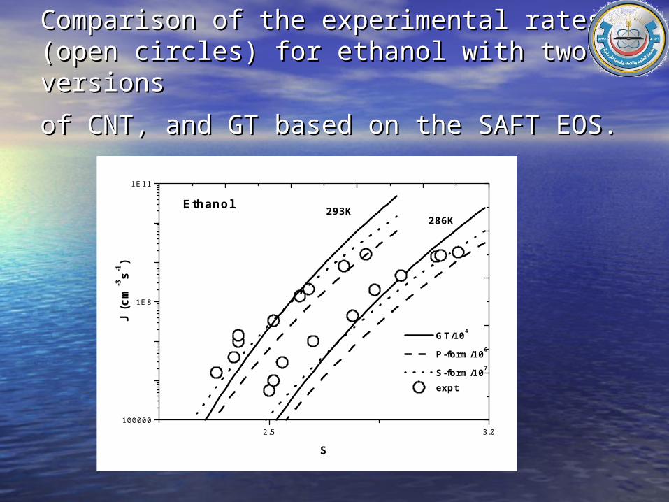
Comparison of the experimental rates Comparison of the experimental rates (open circles) for ethanol with two versions (open circles) for ethanol with two versions

of CNT, and GT based on the SAFT EOS.of CNT, and GT based on the SAFT EOS.

2.5 3.0100000

1E8

1E11

Ethanol

GT/104

P-form/106

S-form/107

expt

J (c

m-3s-1

)

S

286K293K

Number of molecules in critical Number of molecules in critical nucleusnucleus

• Integral EquationIntegral Equation

• CalculationsCalculationshw=35.d0/(steps-1)hw=35.d0/(steps-1)results3=0.0results3=0.0do i=4,steps-3do i=4,steps-3results3=results3+(U(i)-nb)*(i-1)**2*hw**2results3=results3+(U(i)-nb)*(i-1)**2*hw**2end doend doresults3=results3+bb*(U(2)-nb)*(2-1)**2*hw**2results3=results3+bb*(U(2)-nb)*(2-1)**2*hw**2results3=results3+cc*(U(3)-nb)*(3-1)**2*hw**2results3=results3+cc*(U(3)-nb)*(3-1)**2*hw**2results3=results3+aa*(U(steps)-nb)*(steps-1)**2*hw**2results3=results3+aa*(U(steps)-nb)*(steps-1)**2*hw**2results3=results3+cc*(U(steps-1)-nb)*(steps-2)**2*hw**2results3=results3+cc*(U(steps-1)-nb)*(steps-2)**2*hw**2results3=results3+bb*(U(steps-2)-nb)*(steps-3)**2*hw**2results3=results3+bb*(U(steps-2)-nb)*(steps-3)**2*hw**2

ngt=4*pi*results3*hwngt=4*pi*results3*hw

drrrrn b2

0

* 4

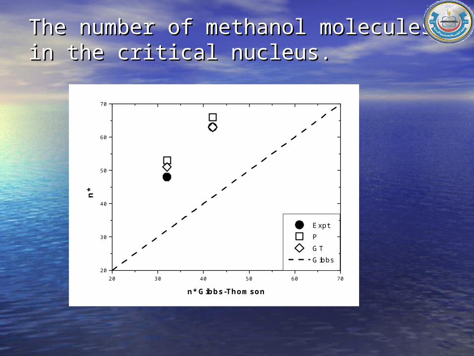
The number of methanol molecules in The number of methanol molecules in the critical nucleus.the critical nucleus.

20 30 40 50 60 7020

30

40

50

60

70

Expt P GT Gibbs

n*

n* Gibbs-Thomson

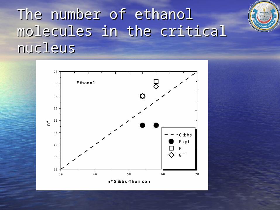
The number of ethanol molecules The number of ethanol molecules in the critical nucleusin the critical nucleus

30 40 50 60 7030

35

40

45

50

55

60

65

70

Ethanol

Gibbs Expt P GT

n*

n* Gibbs-Thomson

ConclusionsConclusions::

• GT improved temperature GT improved temperature dependence of nucleation rates for dependence of nucleation rates for both ethanol and methanol.both ethanol and methanol.

• GT improved supersaturation GT improved supersaturation dependence of nucleation rates dependence of nucleation rates exactly for methanol, but for ethanol, exactly for methanol, but for ethanol, GT couldn’t improve theGT couldn’t improve the

supersaturation dependence of supersaturation dependence of nucleation rates. nucleation rates.

Thank youThank you