Numerical Approximation of

Continuous Traffic Congestion Equilibria

F. Benmansour, G. Carlier, G. Peyre, F. Santambrogio ∗

January 9, 2009

Abstract

Starting from a continuous congested traffic framework recently introduced in [8],we present a consistent numerical scheme to compute equilibrium metrics. We showthat equilibrium metric is the solution of a variational problem involving geodesic dis-tances. Our discretization scheme is based on the Fast Marching Method. Convergenceis proved and numerical results are given.

Keywords: traffic congestion, Wardrop equilibria, eikonal equation, subgradient de-scent, Fast Marching Method.

AMS subject classifications: 49M25, 65K10, 90C25.

1 Introduction

Congestion is an important issue in real-life applications such as road or communicationnetworks. In the early 50’s, Wardrop [15] considered the situation where a large numberof vehicles have to go from one location to another, connected by a finite number ofdifferent roads. Each vehicle has to choose a pathway along the roads to minimize sometransportation cost which depends not only on the chosen pathway but also on the numberof vehicles (the traffic) along it. Naturally, shorter or wider roads are preferred by thevehicles. Nevertheless, the transportation ”cost” on a given road depends increasinglyon the traffic. To avoid the congestion some vehicles may choose a ”longer” pathwayto minimize the cost. Wardrop gave a minimal stability requirement for transportationstrategies: the cost of every actually used pathway should be equal or less than that whichwould be experienced by a single vehicle on any other roads. In particular there is anequilibrium concept: all actually used pathways have the same cost, i.e. they compensatein term of congestion their differences given by length and other conditions. Beside theequilibrium concept there is a minimality concept as well: those pathways are minimalamong all the possible ones. In other words, a Wardrop equilibrium is a situation whereevery traveler uses only shortest paths from his source to his destination, given the overallcongestion pattern resulting from the individual strategies of all the users of the roadnetwork. This natural equilibrium concept, somehow similar to Nash’s equilibrium, hasbeen very popular since its introduction.

Few years later, Beckmann et al. [3] discovered that Wardrop equilibria can be obtainedas minimizers of a certain convex optimization problem. This result is very useful for∗CEREMADE, UMR CNRS 7534, Universite Paris-Dauphine, Pl. de Lattre de Tassigny, 75775 Paris Cedex 16,

FRANCE benmansour, carlier, peyre, santambrogio@ceremade.dauphine.fr.

1

proving theoretical existence, uniqueness and stability results. The convex minimizationformulation (or some dual one) can also be used to compute numerically traffic equilibriaas long as the complexity of the problem is tractable which, in practice, often excludes thecase of large networks. On the contrary, in the present paper, we consider a continuouscase, where there is no network and every path is allowed. Our work is based on acontinuous traffic equilibrium formulation recently introduced in [8]. We will see how thisproblem can be dealt without huge computational costs.

The study of Wardrop equilibria has mainly been restricted to the finite-dimensionalcase where the road network is a given finite graph. In [8], there is no network and con-gestion effects are captured by a metric that depends increasingly on the traffic intensitywhich gives a natural framework to study optimal transportation problems with congestioneffects. It turns out that the problem addressed in [8] can also be interpreted as a continu-ous traffic equilibrium a la Wardrop. The equilibrium problem is then formulated in termsof the traffic intensity or the metric itself. As shown, in section 4, the equilibrium metricis obtained by minimizing some convex functional that is the difference of two terms. Thefirst one is a standard convex integral functional. The second one is a weighted sum ofgeodesic distances between a given source and a given destination as a function of themetric. Building upon this continuous minimization problem, we introduce a discretizedminimization scheme based on Sethian’s FMM [12] (Fast Marching Method). We proveconvergence of the discretized problems to the continuous one and we solve numericallythe discretized problem by an iterative subgradient descent method. Each iteration ofthe discretized problem requires the computation of an element of the subgradient of thegeodesic distance with respect to the current metric. In our companion paper [4], we showhow to compute such a subgradient in the same routine of the FMM algorithm and developother applications of this method.

The continuous traffic congestion model is introduced in section 2. In section 3, trafficequilibria are defined and characterized by means of some convex optimization problem.A more tractable dual formulation is given in Section 4. In section 5, we consider adiscretization of this dual problem, prove that this discretization Γ-converges to the con-tinuous problem and give a consistent numerical scheme to solve the discrete problem.Numerical results are presented in section 6.

2 The model

2.1 Notations and definitions

Given a separable and complete metric space X,M+(X) andM1+(X) denote respectively

the set of positive and finite Borel measures on X and the set of Borel probability measureson X. If X and Y are separable metric spaces, µ ∈ M1

+(X) and f : X → Y is a Borelmap, f]µ denotes the push forward of µ through f i.e. the element of M1

+(Y ) defined byf]µ(B) = µ(f−1(B)) for every Borel subset B of Y .

In the sequel, Ld denotes the d-dimensional Lebesgue measure. If µ and ν are inM+(Rd) then dµ

dν denotes the Radon-Nikodym derivative of µ with respect to ν. We writeµ ν to express that µ is absolutely continuous with respect to ν, in which case, slightlyabusing notations, µ is identified with the Radon-Nikodym derivative dµ

dν .The data of our problem are Ω (modelling a city, say), an open bounded convex subset

of R2, two probability measures, µ0 and µ1 inM1+(Ω), giving respectively the distribution

of residents and services in the city Ω and a transport plan γ i.e. a probability measureon Ω × Ω having µ0 and µ1 as marginals. The transport plan γ models the travelers’

2

everyday movements, more precisely for A and B Borel subsets of Ω, γ(A×B) representsthe fraction of the travelers’ population that commutes from a location in A to a locationin B.

Introducing congestion naturally leads to consider spaces of paths, lengths of suchpaths and sets of probability measures on sets of paths. From now on, we shall denote:

• C := W 1,∞([0, 1],Ω), (endowed with the usual topology of C0([0, 1],R2)),

• Cx,y := σ ∈ C : σ(0) = x, σ(1) = y (x, y in Ω),

• l(σ) :=∫ 1

0 |σ(t)| dt, the length of σ ∈ C,

• for ϕ ∈ C0(Ω,R) and σ ∈ C, we define

Lϕ(σ) :=∫ 1

0ϕ(σ(t))|σ(t)|dt,

• e0(σ) := σ(0), e1(σ) := σ(1), for all σ ∈ C0([0, 1],R2).

Roughly speaking, a transportation strategy is a probability Q over paths (Q(Σ) repre-sents the number of travellers that use a path in Σ) which is compatible with the transportplan γ:

Definition 2.1. A transportation strategy is a probability Q ∈M1+(C) such that (e0, e1)]Q =

γ.

The set of transportation strategies is denoted by

Q(γ) := Q ∈M1+(C) : (e0, e1)]Q = γ.

If ξ ∈ C0(Ω,R+), it is proven in Lemma 2.6 in [8] that the map σ 7→ Lξ(σ) is l.s.c. onC hence Borel for the uniform topology. Since 0 ≤ Lξ(σ) ≤ ‖ξ‖∞l(σ), Lξ ∈ L1(C,Q) assoon as: ∫

Cl(σ)dQ(σ) < +∞ (2.1)

which means that the average (with respect to Q) length is finite. If (2.1) holds thenLξ ∈ L1(C,Q) for every ξ ∈ C0(Ω,R+). If ξ ∈ C0(Ω,R), let us write ξ = ξ+ − ξ− with ξ+

and ξ− the positive and negative part of ξ. Since Lξ = Lξ+ − Lξ− then Lξ is Borel and inL1(C,Q) provided (2.1) holds.

Any Q ∈ M1+(C) induces a traffic intensity which is a nonnegative measure on Ω,

intuitively the traffic intensity of a subregion of Ω is the cumulated traffic of this subregion(or the total amount of mass travelling through the subregion). For simplicity, in the nextdefinition, to avoid the case of measures taking the value +∞, we restrict to the case whereQ satisfies (2.1).

Definition 2.2. Let Q ∈ M1+(C) satisfy (2.1), the traffic intensity of Q is the measure

iQ ∈M+(Ω) defined by:∫Ωϕ(x)diQ(x) :=

∫CLϕ(σ)dQ(σ) =

∫C

(∫ 1

0ϕ(σ(t))|σ(t)|dt

)dQ(σ), (2.2)

for all ϕ ∈ C0(Ω,R).

Let us remark that the total mass of iQ is the average length with respect to Q.

3

2.2 On geodesic distances

For a continuous and nonnegative metric ξ ∈ C0(Ω,R+), the corresponding geodesic dis-tance is denoted cξ

cξ(x, y) := inf Lξ(σ), σ ∈ Cx,y

= inf∫ 1

0ξ(σ(t))|σ(t)|dt, σ ∈ Cx,y

,∀(x, y) ∈ Ω× Ω.

.

A path σ such that Lξ(σ) = cξ(σ(0), σ(1)) is called a geodesic for the metric ξ betweenx = σ(0) and y = σ(1).

In the sequel, we shall need to extend the definitions of cξ and Lξ to the case where ξonly belongs to some Lp space. This is possible when p > 2 (we refer to [8] for details), byproceeding as follows. Let us assume that p > 2 and ξ ≥ 0, ξ ∈ Lp(Ω), then the followingis proved in [8].

Proposition 2.3. Let us assume that p > 2 and define β := 1 − 2/p, then there exists anon-negative constant C such that for every ξ ∈ C0(Ω,R+) and every (x1, y1, x2, y2) ∈ Ω4,one has

|cξ(x1, y1)− cξ(x2, y2)| ≤ C‖ξ‖Lp(Ω)

(|x1 − x2|β + |y1 − y2|β

). (2.3)

Consequently, if (ξn)n ∈ C0(Ω,R+)N is bounded in Lp, then (cξn)n admits a subsequencethat converges in C0(Ω× Ω,R+).

This allows to extend the definition of the geodesic distance cξ to the case ξ ≥ 0 andξ ∈ Lp (with p > 2) as follows:

cξ = supc = lim

ncξn in C0(Ω× Ω) : (ξn)n ∈ C0(Ω), ξn ≥ 0, ξn → ξ in Lp

.

This definition really extends that of geodesic distance since when ξ is continuous andnon-negative, then cξ = cξ (see [8] for details). Section 5.3 shows that this definitioncoincides with a different one, given in terms of pointwise a.e. subsolutions of an EikonalEquation.

It remains to extend the definition of Lξ. To do that, let us define for every q ∈ [1,+∞],the set:

Qq(γ) := Q ∈ Q(γ) : iQ ∈ Lq(Ω) (2.4)

where in the previous definition we have slightly abused notations to intend that iQ L2

and that the density of iQ with respect to L2 is in Lq. If p > 2, ξ ∈ Lp, ξ ≥ 0, (ξn)n is asequence of non-negative continuous functions that converges to ξ in Lp and Q ∈ Qp∗(γ)(p∗ being the conjugate exponent of p), then the following holds (see [8]):

• (Lξn)n converges strongly in L1(C,Q) to some limit which is independent of theapproximating sequence (ξn)n and which is, again, denoted as Lξ.

• The following equality holds:∫Ωξ(x)iQ(x) dx =

∫CLξ(σ) dQ(σ). (2.5)

• The following inequality holds for Q-a.e. σ ∈ C:

Lξ(σ) ≥ cξ(σ(0), σ(1)). (2.6)

Having extended the definition of Lξ and cξ, we naturally call a geodesic any σ ∈ Csuch that Lξ(σ) = cξ(σ(0), σ(1)).

4

2.3 Traffic congestion

Traffic congestion modelling has to capture the fact that travellers spend more time (ormore effort) in regions where the traffic is dense i.e. where the traffic intensity is high. Anatural way to do so (assuming for a moment that iQ L2 with a density with respect toL2 still denoted iQ), is to associate to iQ a metric of the form g(., iQ(.)) where g is a givencongestion function. We shall always assume the following on the congestion function g:

• g ∈ C0(Ω× R+; R+),

• g(x, .) is strictly increasing on R+ for every x ∈ Ω,

• there exists strictly positive constants a and b and a constant α ∈ (0, 1) such that

aiα ≤ g(x, i) ≤ b(iα + 1), ∀i ∈ R+ ∀x ∈ Ω. (2.7)

Let us set q := 1+α and q∗ = 1+1/α its conjugate exponent (note that q∗ > 2 so thatone can define cξ as in the previous paragraph whenever ξ ∈ Lq∗ and ξ ≥ 0) and defineQq(γ) by (2.4). Let us also remark that every Q ∈ Qq(γ) satisfies (2.1). For Q ∈ Qq(γ),the congested metric associated to Q is well-defined and given by:

Definition 2.4. For Q ∈ Qq(γ), the metric associated to Q, denoted ξQ is defined by

ξQ(x) := g(x, iQ(x)), x ∈ Ω. (2.8)

Note that our assumptions on g imply that ξQ ∈ Lq∗

whenever Q ∈ Qq(γ). Sinceq∗ > 2, by the results recalled in paragraph 2.2, cξQ is a well-defined continuous function,LξQ ∈ L1(C,Q) and (2.5) and (2.6) hold for ξ = ξQ.

3 Wardrop Equilibria as solutions of a convex minimizationproblem

3.1 Equilibria

An equilibrium is a transportation strategy Q such that the congested metric ξQ is welldefined (i.e. Q ∈ Qq(γ) with q = α+1 ∈ (1, 2)) and such that, given the congestion result-ing from ξQ, travellers only use shortest paths i.e. geodesics. This stability requirement onthe transportation strategy (all used routes connecting x to y have the same commutingtime and a shorter commuting time than unused routes) was first introduced by Wardrop[15] in the case of a finite number of roads. The generalization to our continuous settingthen reads as:

Definition 3.1. A Wardrop equilibrium is a probability Q ∈ Qq(γ) such that

Q(σ ∈ C : LξQ(σ) = cξQ(σ(0), σ(1))) = 1.

In other words, Q ∈ Qq(γ) is a Wardrop equilibrium if and only if Q gives full mass tothe set of geodesics for the metric ξQ defined by (2.8).

Of course, a necessary condition for the existence of a Wardrop equilibrium, in ourmodel where congestion effects are very strong, is that Qq(γ) is nonempty. As shownin section 3.2, this condition is also sufficient for existence of equilibria. At first glancehowever, the condition Qq(γ) 6= ∅ may seem difficult to check a priori if we only know γ.Yet, in the case when there is a finite number of sources and destinations (which is basicallythe situation considered in our numerical simulations), this condition is automaticallyfulfilled.

5

Proposition 3.2. If γ is a discrete probability measure on Ω×Ω then, for every p ∈ [1, 2),Qp(γ) 6= ∅.

Proof. It is of course enough to prove the claim when γ is a single Dirac mass γ = δ(x0,y0)

and up to a change of coordinates we may assume x0 = (0, 0) and y0 = (1, 0). Now letβ0 > 0 be such that for all β ∈ [0, β0], the curve σβ defined below lies in Ω:

σβ(t) :=

(t, βt) if t ∈ [0, 1/2](t, β(1− t)) if t ∈ [1/2, 1].

We then define dQ := δσβ ⊗ 1[0,β0]dββ0

, of course Q ∈ Q(γ) and Q satisfies (2.1). Forϕ ∈ C0(Ω,R) we then have:∫

Ωϕ(x)diQ(x) =

1β0

∫ β0

0

∫ 1

0ϕ(σβ(t))

√1 + β2 dtdβ

=1β0

∫ β0

0

∫ 1/2

0ϕ(t, βt)

√1 + β2dtdβ +

1β0

∫ β0

0

∫ 1

1/2ϕ(t, β(1− t))

√1 + β2dtdβ

Denoting by T0 the triangle with vertices (0, 0), (1/2, 0), (1/2, β0/2) and performing thechange of variables (β, t)→ σβ(t), the first integral in the expression above equals

1β0

∫T0

ϕ(x, y)1x

√1 +

y2

x2dxdy

and a similar expression gives the value of the second integral. Now remarking that√1 + y2

x2 ≤√

1 + β20 on T0 and that 1/x ∈ Lp(T0,L2) for all p ∈ [1, 2) we get the desired

result.

Remark 3.3. Some techniques from incompressible fluid mechanics, as Yann Brenier pointedout to us, may be used to prove the existence of finite-energy Q′s for more general fixedtransport plan γ′s. In fact, any incompressible measure Q realizing at any time a densityµ and concentrated on L−Lipschitz curves gives rise to a traffic intensity iQ such thatiQ ≤ Lµ. This idea could be used to handle the case of generic transport plans γ from µto µ or, composing with time-dependent diffeomorphism, even from a measure to another.It requires anyway Lp assumptions on the data to get Lp estimates on iQ.

3.2 Existence and characterization of equilibria

Our study of equilibria relies on the following convex optimization problem:

(P) inf∫

ΩH(x, iQ(x))dx : Q ∈ Qq(γ)

(3.1)

where the function H is defined by

H(x, i) :=∫ i

0g(x, s)ds, ∀x ∈ Ω, ∀i ∈ R+. (3.2)

By the same arguments as in [8], one can prove the following.

Theorem 3.4. Assume that Qq(γ) 6= ∅ (q = 1 + α ∈ (1, 2)) then (P) admits at least onesolution.

6

Theorem 3.5. Assume that Qq(γ) 6= ∅ (q = 1 + α ∈ (1, 2)) and let Q ∈ Qq(γ), then Q isan equilibrium if and only if Q solves (P).

Actually, the problem addressed in [8] is slightly different from the one considered here,but all the proofs can be straightforwardly adapted. Indeed, in [8], the transport plan γ isnot given a priori, only its marginals are, a situation slightly more general than the presentone. Also, in [8], the congestion function g only depends on i but it is easy to check thatthe results of Theorems 3.4 and 3.5 extend to the case where g also depends on x underthe assumptions of the present paper.

From now on, we assume that Qq(γ) 6= ∅ (q = 1 + α ∈ (1, 2)). In this case, equilibriaexist and finding them amounts to solve (P). Since H(x, .) is strictly convex, if Q1 andQ2 are equilibria, then necessarily iQ1 = iQ2 . In other words, equilibria are not necessarilyunique but they all induce the same intensity or equivalently the same metric ξ. The nextsection shows that finding the equilibrium metric amounts to solve another optimizationproblem which is dual to (P). This dual problem turns out to be easier than (P) to benumerically handled.

4 Dual formulation

For every x ∈ Ω and ξ ≥ 0, let us define

H∗(x, ξ) := supξi−H(x, i), i ≥ 0, ξ0(x) := g(x, 0).

By our assumptions on g, one has H∗(x, ξ) = 0 for every x ∈ Ω and ξ ≤ ξ0(x), and

1b1/α

(ξ − b)q∗

+

q∗≤ H∗(x, ξ) ≤ 1

a1/α

ξq∗

q∗, ∀x ∈ Ω, ∀ξ ≥ ξ0(x).

Let us recall Young’s inequality:

H(x, i) +H∗(x, ξ) ≥ ξi, ∀i ≥ 0,∀ξ ≥ ξ0(x) (4.1)

and that inequality (4.1) is strict unless ξ = g(x, i) ≥ ξ0(x). In particular, for Q ∈ Qq(γ),we have the identity

H(x, iQ(x)) +H∗(x, ξQ(x)) = ξQ(x)iQ(x) (4.2)

andH(x, iQ(x)) +H∗(x, ξ) > ξiQ(x), ∀ξ ≥ ξ0(x), ξ 6= ξQ(x). (4.3)

Let us now define the functional

J(ξ) =∫

ΩH∗(x, ξ(x))dx−

∫Ω×Ω

cξ(x, y)dγ(x, y) (4.4)

and consider:(P∗) sup

−J(ξ) : ξ ∈ Lq∗ , ξ ≥ ξ0

(4.5)

Theorem 4.1. Let us assume that Qq(γ) 6= ∅ (q = 1 + α ∈ (1, 2)), then

min(P) = max(P∗) (4.6)

and ξ ∈ Lq∗ solves (P∗) if and only if ξ = ξQ for some Q ∈ Qq(γ) solving (P).

7

Proof. Let Q ∈ Qq(γ) (so that ξQ ≥ ξ0) and ξ ∈ Lq∗ with ξ ≥ ξ0, from (4.1) and (2.5) wefirst get: ∫

ΩH(x, iQ(x))dx ≥

∫ΩξiQ −

∫ΩH∗(x, ξ(x))dx

=∫CLξ(σ)dQ(σ)−

∫ΩH∗(x, ξ(x))dx.

Using (2.6) and Q ∈ Qq(γ) we then have∫CLξ(σ)dQ(σ) ≥

∫Cc(σ(0), σ(1))dQ(σ) =

∫Ω×Ω

cξ(x, y)dγ(x, y).

Since Q ∈ Qq(γ) and ξ ∈ Lq∗ , ξ ≥ ξ0 are arbitrary and since we already know that theinfimum of (P) is attained we thus deduce

min(P) ≥ sup(P∗). (4.7)

Now let Q ∈ Qq(γ) solve (P) and let ξ := ξQ (recall that ξQ does not depend on the choiceof the minimizer Q), from Theorem 3.5, we know that

Lξ(σ) = cξ(σ(0), σ(1)) for Q-a.e. σ ∈ C

with (2.5), integrating the previous identity and using Q ∈ Q(γ) we then get:∫ΩξiQ =

∫CLξ(σ)dQ(σ) =

∫Ω×Ω

cξ(x, y)dγ(x, y).

Using (4.2), (4.7) and the fact that Q ∈ Qq(γ) solves (P) yields:

sup(P∗) ≤ min(P) =∫

ΩH(x, iQ(x))dx =

∫ΩξiQ −

∫ΩH∗(x, ξ(x))dx

=∫

Ω×Ωcξ(x, y)dγ(x, y)−

∫ΩH∗(x, ξ(x))dx

so that ξ solves (P∗) and (4.6) is satisfied. Finally if ξ solves (P∗) and Q ∈ Qq(γ) solves(P), then with (2.5) and (2.6), one has∫

ΩξiQ −

∫ΩH∗(x, ξ(x))dx ≥

∫Ω×Ω

cξ(x, y)dγ(x, y)−∫

ΩH∗(x, ξ(x))dx

= max(P∗) = min(P) =∫

ΩH(x, iQ(x))dx

and thus we deduce from (4.1) and (4.3) that ξ = ξQ.

In the sequel, we numerically approximate the unique equilibrium metric ξQ by adescent method on (P∗). One can recover the corresponding equilibrium intensity iQ byinverting the relation ξ(x) = g(x, iQ(x)).

8

5 Discrete Algorithm

The traffic intensity that we are looking for, which is both the optimal one and the uniqueequilibrium, is determined by solving the dual problem in the variable ξ = H ′(i). Thissection describes and justifies a numerical approximation of the optimal ξ in the dualproblem. This procedure (approximating the solution of the dual problem instead of theprimal one) is classical as far as discrete Wardrop problems on networks are concerned (see[1] and the references therein). Obviously our numerical procedure passes itself through adiscretization, but this has nothing to do with the network formulation of discrete Wardropproblem. The discretization of ξ is indeed done on a square lattice and we prove theconvergence of our scheme to the solution of the continuous problem.

5.1 A discrete functional via Fast Marching

This section is concerned with the discrete formulation of the dual problem. After settingthe notations in this discrete setting, the convexity of the discrete functional, with respectto the discrete metric, is proven. The convergence of this discretization to its continuouscounterpart is proven in the next section.

The metric is discretized as a vector ξ = (ξi,j)i,j ∈ RN where ξi,j represents the valueof the metric at a point xi,j = (ih, jh) ∈ Ω of a square lattice. The number of grid pointsis N = h−2. The first term of the energy functional J defined in equation (4.4) is easilydiscretized as h2

∑i,j H

∗(xi,j , ξi,j).The second term of the energy J requires the discretization of the geodesic length cξ.

This can be performed by computing the solution of a discretized Eikonal equation. For afixed source S0, the geodesic distance to S0 is denoted as Uξ(x) = cξ(S0, x). The functionUξ is the viscosity solution of the Eikonal equation

‖∇Uξ‖ = ξ with Uξ(S0) = 0. (5.1)

The vector (Ui,j)i,j is a discretization of the values Uξ(xi,j) of the geodesic distance onthe lattice vertices, where the dependence on ξ is dropped to ease notations. A discreteversion of (5.1) is solved in order to compute U = (Ui,j). For the Eikonal equation, classicfinite difference schemes tend to overshoot and are unstable. Rouy and Tourin [11] showedthat a correct scheme for approximating the viscosity solution for of (5.1) is given by thefollowing first order accurate scheme:

(DxU)2i,j + (DyU)2

i,j = h2(ξi,j)2, (5.2)

where we denote

(DxU)i,j := max(Ui,j − Ui−1,j), (Ui,j − Ui+1,j), 0/h,(DyU)i,j := max(Ui,j − Ui,j−1), (Ui,j − Ui,j+1), 0/h,

and (DU)i,j :=√

(DxU)2i,j + (DyU)2

i,j .

The Fast Marching Method (FMM) is a numerical method introduced by Sethian in [12]for efficiently solving the isotropic Eikonal equation (5.2) on a cartesian grid. Values ofU may be regarded as the arrival times of wavefronts propagating from the source pointS0 with velocity 1/ξ. The central idea behind the FMM is to visit grid points in anorder consistent with the way wavefronts propagate, i.e. with the Huygens principle. Thenumerical complexity of the FMM is O(N log(N)) operations for a grid with N points.

9

Let us call chξ (S0, T ) = U(T ) the value of this solution, computed with FMM, at thetarget point T when the vanishing boundary datum is fixed at S0 and the metric is ξ. Thedependence with respect to the discretization parameter h will be sometimes omitted inthis section, since the lattice is fixed.

The functional to be minimized is the following

Jh(ξ) = h2∑i,j

H∗(xi,j , ξi,j)−∑α,β

chξ (Sα, Tβ)γα,β, (5.3)

where the weights γα,β represent the coupling on the set of pairs sources Sα - targets Tβand

∑α,β γα,β = 1.

Lemma 5.1. The functional Jh is convex.

Proof. The only non trivial point is proving the concavity of the FMM term. It is sufficientto prove that for fixed S0 and T the function ξ 7→ Uξ(T ) is concave in ξ and, thanks to thehomogeneity, it is sufficient to prove super-additivity. We want to prove the inequality

Uξ1+ξ2 ≥ Uξ1 + Uξ2 .

Thanks to the comparison principle of Lemma 5.2 below, it is sufficient to prove thatξ1 + ξ2 ≥ D(Uξ1 + Uξ2). This is easily done if we notice that the operator D is convex (asit is a composition of the function (x, y) 7→

√x2 + y2, which is convex and increasing in

both x and y, and the operator Dx and Dy, which are convex since they are produced asa maximum of linear operators) and 1−homogeneous, and hence it is subadditive.

Lemma 5.2. If ξ ≤ η then Uξ ≤ Uη.

Proof. Let us suppose at first a strict inequality ξ < η. Take a minimum point for Uη−Uξand suppose it is not the fixed point S0. Computing D and using the previously noticedsub-additivity, we have

η = DUη ≤ D(Uη − Uξ) +DUξ = D(Uη − Uξ) + ξ,

which gives D(Uη−Uξ) ≥ η−ξ > 0. Yet, at minimum points we should have D(Uη−Uξ) = 0and this proves that the minimum is realized at S0, i.e. that Uη − Uξ ≥ 0.

To handle the case ξ ≤ η without a strict inequality, just replace η by (1 + ε)η andnotice that the application η 7→ Uη is continuous.

5.2 Description of the algorithm and convergence of its iterations

The discrete function Jh, defined in equation (5.3) is convex and can be minimized usingstandard methods from convex optimization. The first term of the functional Jh is dif-ferentiable, while the second may not be. Hence a subgradient descent algorithm can beused for the discrete optimization problem.

In the following, the dependence of H∗ on the position is omitted to ease notationsand we write H∗(x, ξ) = f(ξ). The functional to optimize is written in the form

Jh(ξ) =∑i,j

f(ξi,j) +K(ξ),

for a regular function f : R+ → R+ and a convex, but in general not C1, function K whichis not separable w.r.t. to the variables ξi,j .

10

The subgradient method corresponds (taking for simplicity ξ0 = g(., 0) = 0) to thefollowing iterative scheme

ξ(1) = 1; ξ(k+1) = max0, ξ(k) − ρkw(k) (5.4)

where (w(k))i,j = f ′(ξ(k)i,j ) + (v(k))i,j ∈ ∂J(ξ(k))

where v(k) ∈ ∂K(ξ(k)) is a vector in the subdifferential of K at the previous point ξ(k) andρk is a suitable sequence of steps.

A well-known result on subgradient algorithms (see for instance [5]) states that thesequence (ξ(k))k converges to the unique minimizer of J (uniqueness comes from strictconvexity) provided the following two constraints are enforced

• The step sizes ρk satisfy∑k

ρk = +∞ and∑k

ρ2k < +∞.

This condition is satisfied for a sequence of steps such as ρk = 1/k.

• The sequence (w(k))k stays bounded, which can be enforced by slightly modifying thepenalty function f . Since K is 1−homogeneous, it is Lipschitz continuous and henceits subgradients are bounded. However, the original penalty f is not necessarilyLipschitz, but, one can consider instead the following Lipschitz function f defined as

f(t) =

f(t) if t ≤ t0,f(t0) + (t− t0)f ′(t0) if t ≥ t0.

It happens that, if t0 is sufficiently large, the minimizers ξ of the modified energyJ and of the original one are the same and satisfy ξi,j ≤ t0. This choice of t0 mayalways be performed as far as f is superlinear at infinity.

A computation of an element v(k) of the subdifferential of K is required for the gradientdescent. Indeed, in [4] a recursive method that computes such a vector in parallel to theiteration of the FMM is detailed. This methods produces a vector which is the gradient ofU w.r.t. ξ at differentiability points and a vector in the subdifferential at all other points.The complexity of this algorithm depends on the complexity of the original FMM, as itvisits the points in the same order. Yet, since it must compute a N−dimensional gradientat each iteration, the result has complexity O(N2 log(N)) for a grid of N points.

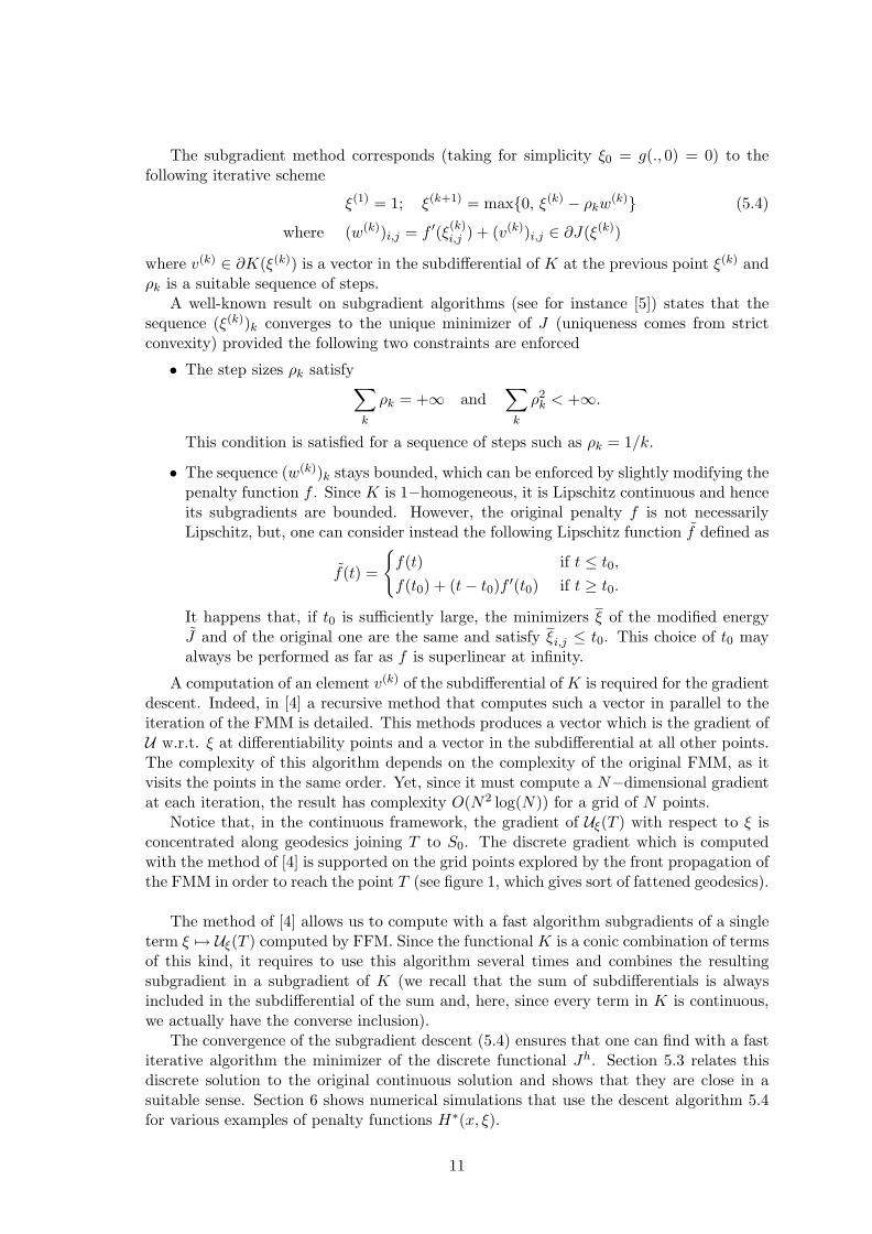
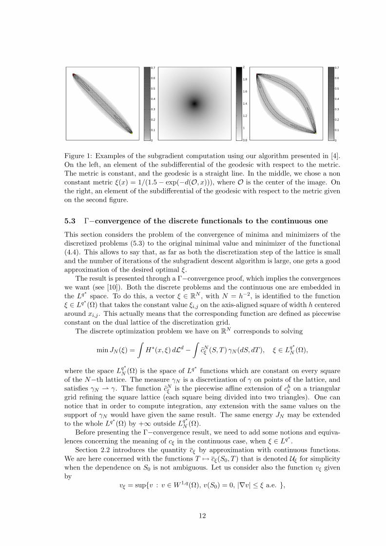
Notice that, in the continuous framework, the gradient of Uξ(T ) with respect to ξ isconcentrated along geodesics joining T to S0. The discrete gradient which is computedwith the method of [4] is supported on the grid points explored by the front propagation ofthe FMM in order to reach the point T (see figure 1, which gives sort of fattened geodesics).

The method of [4] allows us to compute with a fast algorithm subgradients of a singleterm ξ 7→ Uξ(T ) computed by FFM. Since the functional K is a conic combination of termsof this kind, it requires to use this algorithm several times and combines the resultingsubgradient in a subgradient of K (we recall that the sum of subdifferentials is alwaysincluded in the subdifferential of the sum and, here, since every term in K is continuous,we actually have the converse inclusion).

The convergence of the subgradient descent (5.4) ensures that one can find with a fastiterative algorithm the minimizer of the discrete functional Jh. Section 5.3 relates thisdiscrete solution to the original continuous solution and shows that they are close in asuitable sense. Section 6 shows numerical simulations that use the descent algorithm 5.4for various examples of penalty functions H∗(x, ξ).

11

0

0.1

0.2

0.3

0.4

0.5

0.6

0.7

0.8

1

1.2

1.4

1.6

1.8

2

0

0.1

0.2

0.3

0.4

0.5

0.6

0.7

Figure 1: Examples of the subgradient computation using our algorithm presented in [4].On the left, an element of the subdifferential of the geodesic with respect to the metric.The metric is constant, and the geodesic is a straight line. In the middle, we chose a nonconstant metric ξ(x) = 1/(1.5 − exp(−d(O, x))), where O is the center of the image. Onthe right, an element of the subdifferential of the geodesic with respect to the metric givenon the second figure.

5.3 Γ−convergence of the discrete functionals to the continuous one

This section considers the problem of the convergence of minima and minimizers of thediscretized problems (5.3) to the original minimal value and minimizer of the functional(4.4). This allows to say that, as far as both the discretization step of the lattice is smalland the number of iterations of the subgradient descent algorithm is large, one gets a goodapproximation of the desired optimal ξ.

The result is presented through a Γ−convergence proof, which implies the convergenceswe want (see [10]). Both the discrete problems and the continuous one are embedded inthe Lq

∗space. To do this, a vector ξ ∈ RN , with N = h−2, is identified to the function

ξ ∈ Lq∗(Ω) that takes the constant value ξi,j on the axis-aligned square of width h centeredaround xi,j . This actually means that the corresponding function are defined as piecewiseconstant on the dual lattice of the discretization grid.

The discrete optimization problem we have on RN corresponds to solving

min JN (ξ) =∫H∗(x, ξ) dLd −

∫cNξ (S, T ) γN (dS, dT ), ξ ∈ Lq

∗

N (Ω),

where the space Lq∗

N (Ω) is the space of Lq∗

functions which are constant on every squareof the N−th lattice. The measure γN is a discretization of γ on points of the lattice, andsatisfies γN γ. The function cNξ is the piecewise affine extension of chξ on a triangulargrid refining the square lattice (each square being divided into two triangles). One cannotice that in order to compute integration, any extension with the same values on thesupport of γN would have given the same result. The same energy JN may be extendedto the whole Lq

∗(Ω) by +∞ outside Lq

∗

N (Ω).Before presenting the Γ−convergence result, we need to add some notions and equiva-

lences concerning the meaning of cξ in the continuous case, when ξ ∈ Lq∗ .Section 2.2 introduces the quantity cξ by approximation with continuous functions.

We are here concerned with the functions T 7→ cξ(S0, T ) that is denoted Uξ for simplicitywhen the dependence on S0 is not ambiguous. Let us consider also the function vξ givenby

vξ = supv : v ∈W 1,q(Ω), v(S0) = 0, |∇v| ≤ ξ a.e. ,

12

which is the maximal a.e. subsolution of |∇v| = ξ. What we are looking for is very muchlinked to viscosity solution of the Hamilton-Jacobi equation |∇v| = ξ, when ξ is only Lq

∗

(see [6] for a definition via W 1,q test functions and local a.e. inequality and [7] for someother notions and equivalences in the case ξ ∈ L∞). Yet, we are here interested only inthe following two notions: the one presented in [8] (and in Section 2.2) and the maximala.e. one.

Let us prove the following:

Lemma 5.3. We have Uξ := cξ(S0, .) = vξ = limε→0 cξ∗ρε(S0, ·).

Proof. From Lemma 3.5 in [8] we know that there exists a sequence of continuous functions(ξn)n converging to ξ in Lq

∗such that cξn → cξ (in C0 or weakly in W 1,q∗). Since

for continuous functions the equality between cξ(S0, ·) (which equals cξ(S0, ·), thanks toLemma 3.4 in [8]) and vξ is known, we may infer

ξn → ξ in Lq∗(Ω); cξn → cξ in C0(Ω); |∇cξn | ≤ ξn,

which implies at the limit |∇cξ| ≤ ξ. This means that Uξ is an a.e. subsolution of |∇v| = ξ.Consequently, Uξ ≤ vξ.

Let us now take an a.e. subsolution v, i.e. a function v ∈ W 1,q∗(Ω) with |∇v| ≤ ξ.Take a convolution kernel ρε and define vε = v ∗ρε− (v ∗ρε)(S0). We have ∇vε = (∇v)∗ρεand consequently (it depends on the convexity of the norm) |∇vε| ≤ ξ ∗ρε := ξε. Moreovervε(S0) = 0. From these facts we get vε ≤ cξε(S0, ·), as this comes from the equality whichis known for continuous functions (and ξε is continuous). Since (v ∗ ρε)(S0) → 0, passingto the limit as ε→ 0 we get

v ≤ limε→0

cξ∗ρε(S0, ·) + (v ∗ ρε)(S0) = limε→0

cξ∗ρε(S0, ·) ≤ cξ(S0, ·),

the last inequality being justified by the definition of cξ. This proves the thesis, v beingarbitrary.

We can now go through the essential part of the Γ−convergence proof. We denote byUNξN the functions T 7→ cNξN (S0, T ).

Lemma 5.4. Suppose ξN ξ in Lq∗, with ξN ∈ Lq

∗

N (Ω). Then for each S0 the sequence(UNξN )N is bounded in W 1,q∗ and any weak limit u satisifes u ≤ vξ.

Proof. Let us prove boundedness. We consider at first derivatives with respect to thecomponent x of the variable: since UNξN is an affine extension, its ∂/∂x derivative on atriangular cell coincides with the same derivative on the horizontal side of the cell. Theslope on the side is bounded by the value of ξN at one of the vertices. If T is a triangle ofthe partition (its area being A), P1 and P2 are the two vertices we consider and Q1 and Q2

the two squares where ξN is constant (with area 2A each), respectively centered aroundP1 and P2, we get

∫T

∣∣∣∣∣∂UNξN∂x

∣∣∣∣∣q∗

dL2 ≤ AmaxξN (P1)q∗, ξN (P2)q

∗

≤ A(ξN (P1)q∗

+ ξN (P2)q∗) =

12

∫Q1∪Q2

ξq∗

N dL2.

13

Summing up over all triangles any square is counted at most four times, and in the endwe get ∫

Ω

∣∣∣∣∣∂UNξN∂x

∣∣∣∣∣q∗

dx ≤ 2∫

Ωξq∗

N dx.

This proves boundedness (since (ξN )N is bounded in Lq∗

and the same argument may beperformed for ∂/∂y) and the existence of weak limits u (which are uniform limits as well,and hence the condition u(S0) = 0 is conserved).

Let us now define

ξN,x = DxUNξN , ξN,y = DyUNξN , with the property ξN =√ξ2N,x + ξ2

N,y.

Since ξN is bounded in Lq∗, the same is true for ξN,x and ξN,y and we denote by ξx and ξy

their weak limits (up to subsequences). Let us fix an arbitrary rectangle R whose verticesbelong to the N−th lattice. Let us now estimate the positive part of ∂UNξN /∂x on R: inthis case it is sufficient to estimate all ascending slopes. Take an horizontal line in R: allthese slopes coincide with the slopes on the horizontal boundaries of the triangles and arehence bounded by the values of ξN,x at the right extremal points of the segments boundingthe triangles. Fixing the ascending direction allows us to avoid superpositions in the choiceof the extremal point. The same can be done for descending slopes and for vertical slopes.In the case of ascending horizontal slopes we get∫

R

(∂UNξN∂x

)+

dx ≤∫R′N

ξN,x dx ≤∫RξN,x dx+ ||ξN ||Lq∗ |R

′N \R|1/q,

where R′N is a rectangle a little bit larger than R, since it includes all the squares in thedual lattice around the points of ∂R. Yet, |R′N \ R| → 0 as N → ∞. When N → ∞ wecan pass to the limit and obtain∫

R

(∂u

∂x

)+

dx ≤∫Rξx dx,

which, R being arbitrary, implies (∂u

∂x

)+

≤ ξx a.e.

and, taking the maximum over the positive and the negative part,∣∣∣∣∂u∂x∣∣∣∣ ≤ ξx a.e.

This proves |∇u| ≤√ξ2x + ξ2

y .

It is sufficient to prove√ξ2x + ξ2

y ≤ ξ to obtain that u is an a.e. subsolution of theHamilton-Jacobi equation, and hence u ≤ vξ. The inequality we want is a consequence ofstandard properties of weak convergence: if a sequence of vector-valued maps zN (in thiscase, the pairs (ξN,x, ξN,y)) weakly converges to a map z (in this case z = (ξx, ξy)), then,for any convex function f (in this case f(x, y) =

√x2 + y2), f(zN ) h implies f(z) ≤ h

(to prove it, it is sufficient to express f as a supremum of affine functions). The thesis inhence proven.

14

Theorem 5.5. The sequence of functionals JN previously defined Γ−converges with respectto the weak Lq

∗convergence to the limit functional J . Moreover, as the sequence (JN )N is

equi-coercive and every functional, J included, is strictly convex, convergence of the uniqueminimizers and of the values of the minima is guaranteed.

Proof. To prove Γ−convergence it is sufficient to prove that ξN ξ implies lim infN JN (ξN ) ≥J(ξ) and that for every ξ there exists a sequence ξN ξ such that JN (ξN )→ J(ξ).

For proving the first part (Γ−liminf inequality), it is sufficient to notice that the firstaddend in the functionals is lower semicontinuous w.r.t. weak convergence, and that byLemma 5.4, the second behaves the same way (but we have to use the equality providedby Lemma 5.3).

For the second part (Γ−limsup inequality), we know by [10] that it is sufficient toprove it for ξ in a class which is sufficiently dense (“dense in energy”, i.e. so that we canguarantee approximation with convergence of the limit energy J). The class of regularfunctions satisfies this density property. Indeed, by convolution we know that both termsof the functional J converge (for the first it is dominated convergence and for the seconduse Lemma 5.3 again). For regular functions it is a well known fact that we can choose ξNby taking the values of ξ at the points of the lattice and we have uniform convergence ofthe solutions computed by the Fast Marching Method to the true solution of the Eikonalequation (this fact is mainly proved in [11], with techniques coming from [2]; for otherconvergence results on monotone discrete schemes for Hamilton-Jacobi equations see also[9] and [13]).

6 Numerical results

In this section some numerical results are shown. Algorithm described in section 5.2 isused. The equilibrium states are visualized using the metric ξ computed by this algorithm.

The first example consists in a source-target pair (S, T ) and a homogeneous functionalH, which does not depend on the spatial location. As previously seen, ξ = H ′(i), and H ′

is strictly increasing function, thus (at least in the case where H does not depend on x), ξand i are visualized as very similar. In the first example, we took H∗(x, ξ) = 1

3ξ3, so that

H(x, i) = 23 i

32 . On Figure 2 the equilibrium metric on a ”desert” square is shown. Note

that the equilibrium metric is symmetric as the initial configuration of the source and thetarget.

Next, we consider the case where the functional H is spatially varying. We takeH(x, i) = 2

3ξ0(x)i32 (x), where ξ0 is a given fixed congestion metric. Thus H∗(x, ξ) =

13ξ

3/ξ20 . The chosen congestion metric is

ξ0(x) = 1 +A exp(−|x−x0|2

σ21

)+A exp

(−|x−x1|2

σ21

)+B exp

(−|x−x3|2

σ22

)+B exp

(−|x−x4|2

σ22

).

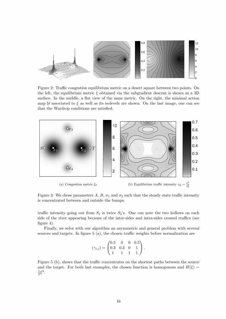
Points xi for i ∈ 1, 2, 3, 4 are chosen in a symmetric manner (see figure 3 (a)). We tookA = 10, B = 4, σ1 = 15 and σ2 = 7 on a square grid of size 100× 100. For figures 2 and3, we used a single source-target pair, thus the traffic weight is γ = 1.

Let us now introduce obstacles and multiple sources and targets. In a symmetricconfiguration of two sources S1 and S2, and two targets T1 and T2; we consider a riverwhere there is no traffic and a bridge linking the two sides of the river (see figure 4 (a)).We chose the traffic weights such that γ1,1 + γ1,2 = 2(γ2,1 + γ2,2) and γ2,2

γ2,1= γ1,1

γ1,2= 2. The

15

0.2

0.4

0.6

0.8

0

2

4

6

8

10

12

Figure 2: Traffic congestion equilibrium metric on a desert square between two points. Onthe left, the equilibrium metric ξ obtained via the subgradient descent is shown as a 3Dsurface. In the middle, a flat view of the same metric. On the right, the minimal actionmap U associated to ξ as well as its isolevels are shown. On the last image, one can seethat the Wardrop conditions are satisfied.

(a) Congestion metric ξ0

0.1

0.2

0.3

0.4

0.5

0.6

0.7

(b) Equilibrium traffic intensity iQ = ξ2

ξ20

Figure 3: We chose parameters A, B, σ1 and σ2 such that the steady state traffic intensityis concentrated between and outside the bumps.

traffic intensity going out from S1 is twice S2’s. One can note the two hollows on eachside of the river appearing because of the inter-sides and intra-sides crossed traffics (seefigure 4).

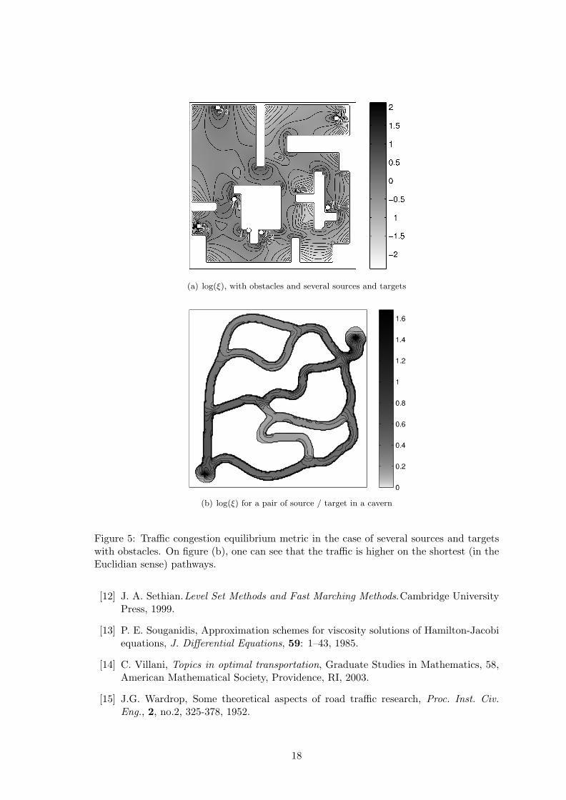
Finally, we solve with our algorithm an asymmetric and general problem with severalsources and targets. In figure 5 (a), the chosen traffic weights before normalization are

(γi,j) =

0.5 0 0 0.50.3 0.3 0 11 1 1 1

.

Figure 5 (b), shows that the traffic concentrates on the shortest paths between the sourceand the target. For both last examples, the chosen function is homogenous and H(ξ) =13ξ

3.

16

(a) 3D view of ξ

−2

−1.5

−1

−0.5

0

0.5

(b) Flat view of log(ξ)

Figure 4: Two sources and two targets, with a river and a bridge on a symmetric config-uration with asymmetric traffic weights.

References

[1] J.-B. Baillon and R. Cominetti, Markovian Traffic Equilibrium, Math. Prog., 111,no. 1-2, 33–56, 2008.

[2] G. Barles and P. E. Souganidis, Convergence of approximation schemes for fullynonlinear second order equations, Asymptotic Anal., 4: 271–283, 1991.

[3] M. Beckmann, C. McGuire and C. Winsten, C., Studies in Economics of Transporta-tion. Yale University Press, New Haven, 1956.

[4] F. Benmansour, G. Carlier, G. Peyre and F. Santambrogio, Derivatives with respectto metrics and applications: Subgradient Marching Algorithm, preprint available athttp://cvgmt.sns.it/people/santambro.

[5] J.F. Bonnans, J.C. Gilbert, C. Lemarechal and C. Sagastizabal, Numerical Opti-mization, 2nd Edition, Springer-Verlag, Heidelberg, 2006.

[6] L. Caffarelli, M. G. Crandall, M. Kocan and A. Swiech, On Viscosity Solutions ofFully Nonlinear Equations with Measurable Ingredient, Comm. on Pure and Appl.Math., 49 (4): 365–398, 1999.

[7] F. Camilli and E. Prados, Shape-from-Shading with discontinuous image brightness,Appl. Num. Math., 56 (9): 1225–1237, 2006.

[8] G. Carlier, C. Jimenez , F. Santambrogio, Optimal transportation with traffic conges-tion and Wardrop equilibria, SIAM Journal on Control and Opt. 47 (3): 1330–1350,2008.

[9] M. G. Crandall and P.-L. Lions, Two approximations of solutions of Hamilton-Jacobiequations, Math. Comp., 43: 1–19, 1984.

[10] G. Dal Maso: An Introduction to Γ−convergence. Birkhauser, Basel, 1992.

[11] E. Rouy and A. Tourin. A viscosity solution approach to shape from shading. SIAMJournal on Numerical Analysis, 29:867–884, 1992.

17

(a) log(ξ), with obstacles and several sources and targets

(b) log(ξ) for a pair of source / target in a cavern

Figure 5: Traffic congestion equilibrium metric in the case of several sources and targetswith obstacles. On figure (b), one can see that the traffic is higher on the shortest (in theEuclidian sense) pathways.

[12] J. A. Sethian.Level Set Methods and Fast Marching Methods.Cambridge UniversityPress, 1999.

[13] P. E. Souganidis, Approximation schemes for viscosity solutions of Hamilton-Jacobiequations, J. Differential Equations, 59: 1–43, 1985.

[14] C. Villani, Topics in optimal transportation, Graduate Studies in Mathematics, 58,American Mathematical Society, Providence, RI, 2003.

[15] J.G. Wardrop, Some theoretical aspects of road traffic research, Proc. Inst. Civ.Eng., 2, no.2, 325-378, 1952.

18