Numerical Continuation Applied to Landing Gear

Mechanism Analysis

J. A. C. Knowles∗† B. Krauskopf† and M. H. Lowenberg∗

Faculty of Engineering, University of Bristol, UK

A method of investigating quasi-static mechanisms is presented and applied to an overcentremechanism and to a nose landing gear mechanism. The method uses static equilibriumequations along with equations describing the geometric constraints in the mechanism. Inthe spirit of bifurcation analysis, solutions to these steady-state equations are then contin-ued numerically in parameters of interest. Results obtained from the bifurcation methodagree with the equivalent results obtained from two overcentre mechanism dynamic models(one state-space and one multibody dynamic model), whilst a considerable computationtime reduction is demonstrated with the overcentre mechanism. The analysis performedwith the nose landing gear model demonstrates the flexibility of the continuation approach,allowing conventional model states to be used as continuation parameters without a needto reformulate the equations within the model. This flexibility, coupled with the compu-tation time reductions, suggests that the bifurcation approach has potential for analysingcomplex landing gear mechanisms.

I. Introduction

Mechanisms are structures that move in a pre-determined and controlled manner. They make up anessential part of any aircraft, performing jobs as diverse as deploying aerodynamic surfaces or allowingpassengers to adjust their seats. The landing gear mechanism is of particular importance, its purpose beingto enable the wheels of an aircraft to move between retracted and deployed states when required to do soby the pilot. To this end, the mechanism needs to downlock to withstand ground loads on touchdown andwhilst taxiing. The primary way to deploy and downlock the landing gear is by means of the landing gearactuator, which deploys the gear in a steady and controlled manner. Regulations require a secondary meansof deploying the landing gear, to be used should the primary actuator fail to operate. Generally, the simplestand most efficient option is to use gravity as the secondary deployment mechanism: the landing gear simplyfalls out of the body of the aircraft, and the mechanism downlocks under the freefall motion of the landinggear.

All landing gear mechanism designs must operate reliably in both normal and emergency situations.For a conventional main landing gear with a single side stay, the analysis of its operation under differentoperational conditions is challenging. With the increasing use of composite materials in aircraft primarystructural components, dual sidestay landing gears are being developed to facilitate main landing gearintegration within a composite wing box structure. The dual sidestay landing gear is a more complicatedmechnism, and presents new challenges to ensure downlocking of both sidestays under any operationalconditions, including freefall emergency deployment.

Most of the research into landing gear modelling focuses on dynamic modelling of structural aspects,1,2

whereas the analysis of landing gear mechanisms is much less prevalent in the literature. Mathematicalanalysis of landing gear mechanisms primarily deals with the geometric design of the mechanism, i.e. how toallow the gear to move between two positions (retracted and deployed) within stowed space constraints.3–5

The standard approach used by industry to investigate landing gear mechanisms is to perform multiple timehistory simulations. A slowly varying (quasi-static) force is applied to unlock the lock links, and then re-lockthe lock links. The value at which they re-lock is referred to as the downlock force, signified when the∗Department of Aerospace Engineering†Department of Engineering Mathematics

1 of 15

American Institute of Aeronautics and Astronautics

angle between the two lock links jumps through 180◦. Another parameter of interest, such as the side-stayattachment point, can then be changed before the simulation is repeated. This time history approach usescomplex models and requires a large amount of computation time to investigate the system, because a newsimulation has to be run every time a parameter value is changed. The choice of parameter that can bevaried continuously is also limited; in this instance to the force applied to the lock-links.

An alternative to this ‘brute force’ computational method is proposed here, which makes use of conceptsfrom the theory of dynamical systems; see6–8 as exemplars for background information. Several recentapplications of dynamical systems methods have demonstrated the advantages that they can offer in anaerospace context; this includes the analysis of aircraft ground dynamics9 and the study of nose landinggear shimmy.10 Here, the mechanism configuration and internal force distribution is formulated as a systemof coupled equations, which are inherently nonlinear due to the geometric constraints. The steady-statesolutions of these equations can then be found and followed, or continued, in parameters of interest withstandard numerical continuation software such as the package AUTO.11 A particular advantage of thiscoupled-equation approach is that any model state (such as an angle between links) or parameter (such as anapplied force) can be used as the main continuation parameter without needing to reformulate the governingequations as a function of this main parameter. It is this flexibility, in combination with a substantially lowercomputational cost, that makes the continuation approach appealing for the analysis of even complicatedlanding gear mechanisms. The method is first demonstrated in Section II for an overcentre mechanism; thissimple example, consisting of a system of 6 equations, is used to compare the dynamic simulation and thenumerical continuation approaches. In Section III the continuation method is demonstrated with a noselanding gear model described by a system of 25 equations. This more realistic example demonstrates theversatility of the new method to analyse landing gear downlock loads.

II. The Overcentre Mechanism

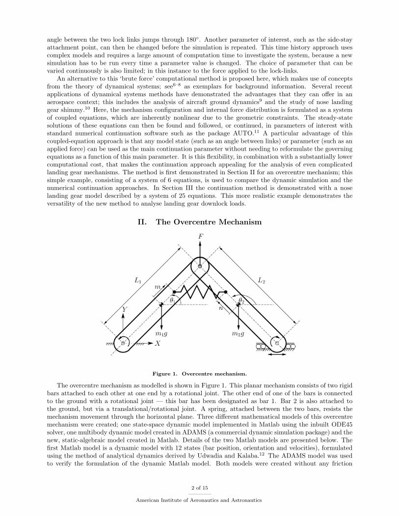
Figure 1. Overcentre mechanism.

The overcentre mechanism as modelled is shown in Figure 1. This planar mechanism consists of two rigidbars attached to each other at one end by a rotational joint. The other end of one of the bars is connectedto the ground with a rotational joint — this bar has been designated as bar 1. Bar 2 is also attached tothe ground, but via a translational/rotational joint. A spring, attached between the two bars, resists themechanism movement through the horizontal plane. Three different mathematical models of this overcentremechanism were created; one state-space dynamic model implemented in Matlab using the inbuilt ODE45solver, one multibody dynamic model created in ADAMS (a commercial dynamic simulation package) and thenew, static-algebraic model created in Matlab. Details of the two Matlab models are presented below. Thefirst Matlab model is a dynamic model with 12 states (bar position, orientation and velocities), formulatedusing the method of analytical dynamics derived by Udwadia and Kalaba.12 The ADAMS model was usedto verify the formulation of the dynamic Matlab model. Both models were created without any friction

2 of 15

American Institute of Aeronautics and Astronautics

to ensure that they would match provided the state-space equations of the Matlab model were formulatedcorrectly. The static algebraic model has 6 states (bar centre of gravity positions and orientations) and isformulated from the geometric constraints and Newtonian force/equilibrium equations. The continuationsoftware package AUTO11 is used to solve this system of algebraic equations by tracing solutions to thesteady state equations as a parameter is varied continuously.

A. State-space Dynamic Model

The state-space dynamic model of an overcentre mechanism was used as the baseline against which toevaluate the static model. The equations of motion were constructed using the fundamental equation asderived by Udwadia and Kalaba;12 following their notation:

x = a +M−12 (AM−

12 )+(b−Aa) (1)

Here:x = [x1,y1,θ1,x2, y2,θ2]T ;a is a (q × 1) external acceleration vector of the unconstrained system (where q is the number of states,which is 6 for the overcentre mechanism);b is a (p × 1) vector from the right-hand side of (appropriately differentiated) constraint equations whenwritten in the form A(x, x, t)x = b(x, x, t) where p = the number of states minus the system degrees offreedom (D.o.F);M is the (q × q) mass/inertia matrix of the system;I is the (q × q) identity matrix;A is the (p× q) matrix from the left-hand side of the constraint equation.

Terms with a superscript ‘+’ are the Morse-Penrose (M-P) inverse of that matrix. The Matlab function pinvis used to calculate this inverse in the model; for more information on the M-P inverse see12 .

The system constraints at the bar ends are specified from the geometry as

x1 − L12 cos θ1 = 0

y1 − L12 sin θ1 = 0

x1 + L12 cos θ1 − (x2 + L2

2 cos θ2) = 0y1 + L1

2 sin θ1 − (y2 + L22 sin θ2) = 0

y2 − L22 sin θ2 = 0

(2)

Equations (2) are differentiated twice with respect to time before being re-arranged into the form A(t, x)x =b(t, x, x) to yield

1 0 L12 sin θ1 0 0 0

0 1 −L12 cos θ1 0 0 0

1 0 −L12 sin θ1 −1 0 L2

2 sin θ20 1 L1

2 cos θ1 0 −1 −L22 cos θ2

0 0 0 0 1 −L22 cos θ2

x1

y1

θ1

x2

y2

θ2

=

−L1

2 θ12

cos θ1−L1

2 θ12

sin θ1L12 θ1

2cos θ1 − L2

2 θ22

cos θ2L12 θ1

2sin θ1 − L2

2 θ22

sin θ2−L2

2 θ12

sin θ2

. (3)

The matrix A and vector b from the left- and right-hand side (respectively) of Eq. (3) can then be usedin the fundamental equation (1).

The applied acceleration vector a contains both the gravitational acceleration g and the spring accelera-tion as. Gravity was assumed to act in the negative y-direction with a value of 9.81m/s2, whilst the springacceleration follows the standard differential equation for a linear spring, Mrx+cx+k = 0. The accelerationcaused by the spring is applied between the spring attachment points at distances m and n from the centreof gravity (C.G.) positions of the left- and right-hand bars, respectively; see Figure 1. For simplicity, initialvalues of 0 for m and n were used, resulting in the applied acceleration vector

a =[as −g 0 as −g 0

]T. (4)

3 of 15

American Institute of Aeronautics and Astronautics

The acceleration caused by the spring force is given by

as = −M−1r

(k(1− R

L)H

[x1

x2

]+ cH

[x1

x2

]). (5)

Here:

Mr is the reduced mass matrix, containing just the bar masses

[m1 00 m2

];

k is the spring stiffness;R is the unstretched spring length;L is the spring length;

H is the direction matrix used to assign acceleration direction:

[1 −1

−1 1

];

c is the damping coefficient.

B. Static Model

The static model is formulated as a system of simultaneous algebraic equations. The six states are assumedto be independent, with the equations providing the dependencies given by

x1 − L12 cos θ1 = 0

y1 − L12 sin θ1 = 0

x2 + L22 cos θ2 −

(x1 + L1

2 cos θ1)

= 0y2 + L2

2 sin θ2 −(y1 + L1

2 sin θ1)

= 0y2 − L2

2 sin θ2 = 0Fsx1

[(12 −

mL1

)tan θ1 −

(12 −

nL2

)tan θ2

]+ Fsy1

(mL1− n

L2

)+ 1

2 (w1 + w2)− F = 0

(6)

The first five rows of Eq. (6) provide the inter-state dependencies and would be sufficient to describe thegeometry of the system if a single state was specified. They have been derived in the same way as thoseused to create the dynamic model, given in Eq. (2). The final row results from the static force/momentequilibrium which the mechanism is assumed to maintain in a steady-state. This last constraint enables theinclusion of the overcentre mechanism force F , which is initially chosen as the user-varied system parameter.

Figure 2. Free-body diagram of overcentre mechanism.

4 of 15

American Institute of Aeronautics and Astronautics

Figure 2 shows the free-body diagram for the components of the overcentre mechanism which were usedto construct the static force/moment equilibrium equations for the static model. The moment equilibriumequations for each bar in terms of the bars’ orientations θ1 and θ2, the gravitational forces on the bars m1gand m2g and the spring force components in the global x- and y-directions Fsx and Fsy, are[

L2R21y − L2

2 m2g + F 2sy

(L22 + n

)]cos θ2 −

[L2R

21x +

(L22 + n

)F 2

sx

]sin θ2 = 0[

L1(R12y + F )− L1

2 m1g + F 1sy

(L12 +m

)]cos θ1 −

[L1R

12x +

(L12 +m

)F 1

sx

]sin θ1 = 0

}(7)

Moments were taken about the ground attachment points for each bar to remove the need to include all thereaction forces in the force expression. Due to the nature of the prismatic/rotational joint at the groundpoint of bar 2, the horizontal ground force R2

x = 0, so resolving horizontally for bar 2 provides the relationR21

x = −F 2sx.

C. Comparison of Static and Dynamic Equation Formulation

Results obtained from the three overcentre models are presented in this section. An investigation is used todemonstrate the efficiency of the new method using the static-algebraic formulation when compared to thetraditional approach.

1. Overcentre Mechanism Model Validation

.

.

40 30 20 10 0 10 20 30 40 50 601.5

1

0.5

0

0.5

1

1.5

(a)θ1

[rad]

Applied Force [N ] F

!"

(b)θ1

[rad]

Applied Force [N ] F

S

S

Figure 3. Comparison of quasi-static analysis results from: (a) dynamic models in ADAMS (grey curve) andMatlab (black curve), (b) static algebraic model — stable solutions are indicated by the solid curves.

Figure 3 compares results from three different models. Figure 3(a) shows results from the two dynamicmodels (in ADAMS and Matlab), where the applied force (F ) was gradually decreased and then increasedover the displayed range. This figure shows perfect agreement between the two dynamic models over theentire range of applied force F . Because of this agreement, the Matlab model was used when comparing

5 of 15

American Institute of Aeronautics and Astronautics

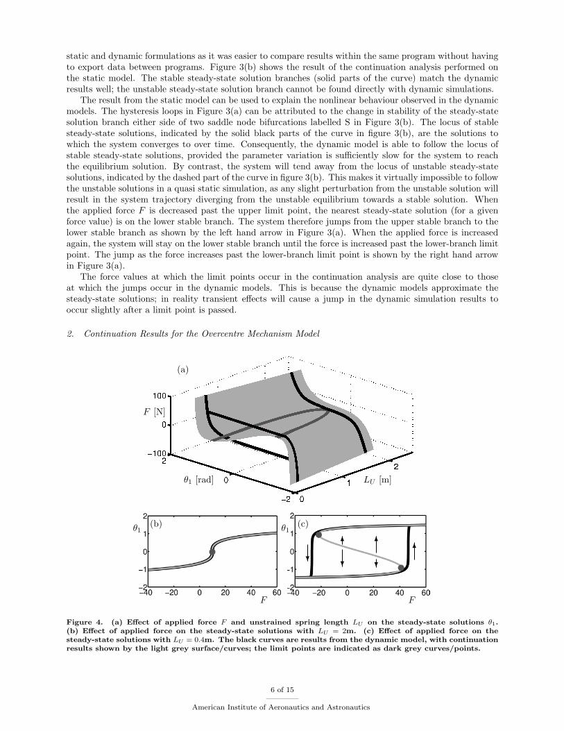
static and dynamic formulations as it was easier to compare results within the same program without havingto export data between programs. Figure 3(b) shows the result of the continuation analysis performed onthe static model. The stable steady-state solution branches (solid parts of the curve) match the dynamicresults well; the unstable steady-state solution branch cannot be found directly with dynamic simulations.

The result from the static model can be used to explain the nonlinear behaviour observed in the dynamicmodels. The hysteresis loops in Figure 3(a) can be attributed to the change in stability of the steady-statesolution branch either side of two saddle node bifurcations labelled S in Figure 3(b). The locus of stablesteady-state solutions, indicated by the solid black parts of the curve in figure 3(b), are the solutions towhich the system converges to over time. Consequently, the dynamic model is able to follow the locus ofstable steady-state solutions, provided the parameter variation is sufficiently slow for the system to reachthe equilibrium solution. By contrast, the system will tend away from the locus of unstable steady-statesolutions, indicated by the dashed part of the curve in figure 3(b). This makes it virtually impossible to followthe unstable solutions in a quasi static simulation, as any slight perturbation from the unstable solution willresult in the system trajectory diverging from the unstable equilibrium towards a stable solution. Whenthe applied force F is decreased past the upper limit point, the nearest steady-state solution (for a givenforce value) is on the lower stable branch. The system therefore jumps from the upper stable branch to thelower stable branch as shown by the left hand arrow in Figure 3(a). When the applied force is increasedagain, the system will stay on the lower stable branch until the force is increased past the lower-branch limitpoint. The jump as the force increases past the lower-branch limit point is shown by the right hand arrowin Figure 3(a).

The force values at which the limit points occur in the continuation analysis are quite close to thoseat which the jumps occur in the dynamic models. This is because the dynamic models approximate thesteady-state solutions; in reality transient effects will cause a jump in the dynamic simulation results tooccur slightly after a limit point is passed.

2. Continuation Results for the Overcentre Mechanism Model

.

.

(a)

F [N]

θ1 [rad] LU [m]

(b)

F

θ1(c)

F

θ1

!"

!

" "

!

Figure 4. (a) Effect of applied force F and unstrained spring length LU on the steady-state solutions θ1.(b) Effect of applied force on the steady-state solutions with LU = 2m. (c) Effect of applied force on thesteady-state solutions with LU = 0.4m. The black curves are results from the dynamic model, with continuationresults shown by the light grey surface/curves; the limit points are indicated as dark grey curves/points.

6 of 15

American Institute of Aeronautics and Astronautics

Figure 4 shows a surface of steady-state solutions in terms of the angle θ1, the applied force F and theunstrained spring length LU , along with a locus of the limit points. Both were computed by continuationanalysis of the static equation formulation. For comparison, multiple quasi-static simulation runs using thedynamic Matlab model were performed for different unstrained spring lengths; two examples are shown asthe black curves in Figure 4. The grey surface was created from multiple continuation runs of the staticmodel at discrete unstrained spring lengths, which were interpolated appropriately to produce the surface.

The effect of the limit point can be described by comparing the system response as the applied forceis slowly varied. Figure 4(b) shows that, for a given applied force (e.g. 20N), there is a single steady-stateequilibrium to which the system will be attracted. If this applied force is slowly decreased, the systemwill follow the black curve (plotted under the light grey curve) which traces out the locus of equilibriaas obtained by the continuation analysis (the grey curve). For all applied force values, there is a uniqueequilibrium solution which is stable. This is because, as the mechanism is downlocked, the spring remainsin compression, so the spring force exerted on the links acts in a constant direction.

Figure 4(c) shows that for a shorter unstrained spring length, two limit point bifurcations appear. Thesebifurcations indicate that there is a change in stability properties of the equilibrium solutions either side of thebifurcation. For this case, an applied force of 20N has two stable equilibrium solutions (the top and bottomcurves, shown to be stable because the black, dynamic simulation curve follows these branches) separatedby a branch of unstable equilibria. This means that the equilibria to which the system will be attracted ina time history simulation depends on the initial conditions — if the initial system angle (for a given forcevalue) is below the unstable curve, the mechanism will tend towards the lower stable branch, whereas foran initial angle above the unstable branch it will tend towards the top stable brancha. Considering the casewhen the system starts on the top stable branch as described in the previous section, if the force is decreasedthe system will follow the black curve which traces the steady-state solutions up to the limit point. If theapplied force is increased past the limit point, the system will tend to the single equilibrium which exists onthe lower branch, similarly to the case shown in Figure 3. This means that the force at which a limit pointbifurcation occurs is the minimum force required to downlock the mechanism.

Even on the level of a two-parameter analysis, the static formulation provides similar results to thedynamic simulations performed in ADAMS. Some of the key advantages of using the static formulationmethod become apparent when considering the flexibility and ease of computing such surfaces. The ADAMSresults are an order of magnitude slower to compute than the continuation results for the same surface.Furthermore, the continuation analysis is able to compute the regions of unstable behaviour bounded by thefold curve without any problem.

aThis type of interpretation requires caution when applied to a multi-DoF system, as a point lying between stable andunstable loci in one projection may not reflect its overall position in full state-space.

7 of 15

American Institute of Aeronautics and Astronautics

D. Two-parameter Continuation of the Limit Point Locus

.

.

(a)

Fold curve!!"

F [N]

θ1 [rad] LU [m]

(b)θ1

Fold curve!"

#$

LU

(c)F

Fold curve!"

#$

LU

Cusp point!!"

Figure 5. (a) Limit point trace for varying unstrained spring length LU , and its projections in the plane of(b) link-1 angle θ1 versus unstrained spring length LU plane and (c) applied force F versus unstrained springlength LU .

The flexibility of the static formulation is evident when considering the locus of limit points plottedin Figure 5; this locus is also shown in Figure 4. Importantly, it can be computed directly by using two-parameter continuation without the need to produce a surface of equilibria. Since a bifurcation point has aparticular mathematical expression, this expression can be used (effectively) as another system constraint.This allows two parameters to be used as continuation parameters, hence ‘two-parameter continuation’.For the overcentre mechanism, the limit point locus was computed by tracing the limit point in terms ofthe unstrained spring length LU whilst allowing the force F to vary appropriately to maintain equilibrium.Figures 5(b) and (c) show projections of how the two ‘dependent’ variables, applied force F and the angleof bar one θ1, vary as the unstrained spring length LU is continued. The downlock force value for a givenunstrained spring length is found by considering the lower branch of saddle node bifurcations in Figure 5(c).Referring back to Figure 4(c), any initial system configuration with an equilibrium on the top stable branchwill remain on this branch unless the applied force is decreased below the upper limit point. In Figure 5(c),the projection shown in Figure 4(c) would appear as a vertical trajectory. Hence, as the force is decreasedthe overcentre mechanism will remain on the upper branch until the applied force reaches the lower foldcurve, when the ‘jump’ in link angle would occur. From a design perspective, this projection could be usedwith relative ease to determine upper and lower bounds on the unstrained spring length in dependence ondownlock load requirements. For example, if it was desired that the overcentre mechanism must downlockfrom any position without applying any external forces (i.e. F ≥ 0), Figure 5(c) shows that this can only beachieved for unstrained spring lengths approximately greater than 1.2 m.

Apart from reducing the computational workload, continuing the limit point ensures comprehensivecoverage of the underlying steady-state system behaviour, whereas interpolating between results for discretespring length values may miss highly nonlinear behaviour.

8 of 15

American Institute of Aeronautics and Astronautics

III. Nose Landing Gear Mechanism

Similarly to the static model of an overcentre mechanism (as described in Section IIB), the equationsfor the static landing gear model are formulated as a set of algebraic equations with 15 bar position androtation states (all assumed to be independent). This simplified landing gear mechanism consists of 5 bars,connected to one another by planar revolute joints. The points where the gear attaches to the aircraft are,for the purposes of this model, assumed to be fixed in space. The main fitting attachment point was chosenas the global co-ordinate system origin. The layout of the landing gear, along with various state variablesand parameters associated with it, is sketched in Figure 6.

A. Static Model

Figure 6. Sketch of a nose landing gear in downlocked position.

Unlike for the overcentre mechanism the force/moment equilibrium conditions are too complicated toexpress as a single constraint equation. It was therefore necessary to introduce extra states (representingthe inter-link forces) to allow the force and moment equilibrium equations for each bar to be expressed asan individual constraint.

9 of 15

American Institute of Aeronautics and Astronautics

The resulting system of states and equations consists of:

• 10 position (x, y) co-ordinates of the centres of gravity of the 5 links;

• 5 rotation (θ) co-ordinates of the links’ orientations to the positive x-axis;

• 14 equations to constrain each bar end to a given point;

• 18 inter-link forces;

• 4 ground-link forces;

• 1 applied actuator force;

• 10 static force equilibrium equations;

• 5 moment equilibrium equations;

• 8 force equilibrium equations at link joints.

There are therefore 37 equations described in terms of 37 states and several parameters. When performinga continuation run, AUTO requires 37 states and one additional continuation parameter to be determinedby 37 equations. By using static equilibrium equations it is possible to use any model state or parameter asthe continuation parameter, provided there are still 37 variables to be determined.

To reduce the complexity, it is possible to remove eight inter-link forces by applying the eight forceequilibrium equations at link joints directly. The description of the four ground-link forces requires fourequations, so a further four equations and states can be removed. These two simplifications reduce thesystem by 12 equations and 12 forces, resulting in a system of 25 equations with 25 states and severaladditional parameters. The geometric constraints are:

x1 −Ax − L12 cos θ1 = 0

y1 −Ay − L12 sin θ1 = 0

x1 − x2 + L12 cos θ1 + L2

2 cos θ2 = 0y1 − y2 + L1

2 sin θ1 + L22 sin θ2 = 0

x2 − x3 + L22 cos θ2 − L23

2 cos (θ3 + ψ1) = 0y2 − y3 + L2

2 sin θ2 − L232 sin (θ3 + ψ1) = 0x3 + L3

2 cos θ3 = 0y3 + L3

2 sin θ3 = 0x1 − x4 + L1

2 cos θ1 + ll12 cos θ4 = 0

y1 − y4 + L12 sin θ1 + ll1

2 sin θ4 = 0x4 − x5 + ll1

2 cos θ4 + ll22 cos θ5 = 0

y4 − y5 + ll12 sin θ4 + ll2

2 sin θ5 = 0x5 − x3 + ll2

2 cos θ5 − L352 cos (θ3 − ψ2) = 0

y5 − y3 + ll22 sin θ5 − L35

2 sin (θ3 − ψ2) = 0

(8)

The various elements within the force/moment equilibrium equations can be expressed in the matrixform AF −B = 0, where F is a vector of the inter-link forces, A is a matrix of force coefficients and B is avector of the remaining terms. We have:

10 of 15

American Institute of Aeronautics and Astronautics

A =

sθ1 −cθ1 0 0 0 0 sθ1 −cθ1 0 0 01 0 −1 0 0 0 0 0 0 0 00 1 0 −1 0 0 0 0 0 0 00 0 sθ2 −cθ2 0 0 0 0 0 0 00 0 [C](1) [C](2) [C](3) [C](4) 0 0 0 0 00 0 0 0 0 0 1 0 1 0 00 0 0 0 0 0 0 1 0 1 10 0 0 0 0 0 0 0 sθ4 −cθ4 − 1

2cθ4

0 0 0 0 −1 0 0 0 1 0 00 0 0 0 0 −1 0 0 0 1 00 0 0 0 sθ5 −cθ5 0 0 0 0 0

, (9)

where s ≡ sin, c ≡ cos and

[C] =

L32 sin(θ3 + ψ1)− L3

2 sin θ3L32 cos θ3 − L32 cos(θ3 + ψ1)L35 sin(θ3 − ψ1)− L3

2 sin θ3L32 cos θ3 − L35 cos(θ3 − ψ1)

T

, (10)

B =

m12 g cos θ1

0m2gm22 g cos θ2−m3

2 gL3 cos θ3 − [lsp2 sin(θ3 + ψ3)− L32 sin θ3]F x

s3 + [lsp2 cos(θ3 + ψ3)− L32 cos θ3]F y

s3 +D

−F xs4

m4g − F ys4

12F

ys4(1− lsp1

L4) cos θ4 − 1

2Fxs4(1− lsp1

L4) sin θ4 − m4

2 g cos θ40−m5g

−m52 g cos θ5

, (11)

withD =

14ρ(U∞ cos(α− θ3 +

π

2)2d(L2

3)CD . (12)

Here:ρ is the air density at sea level = 1.225 kg

m3 ;U∞ is the air velocity;α is the angle between the airflow direction and the global x-axis, initially set to zero;d is the diameter of the main fitting;CD is an estimate of the drag coefficient of the main fitting of the landing gear = 1.17b.

By expressing the force equilibrium equations in this way, initialising the solution when matrix A and vectorB are known only requires computing F = A−1B.

B. Downlock Force Analysis

This section demonstrates how the continuation approach can be used to determine the downlock forcerequired to engage the lock links for a planar nose landing gear mechanism under different aerodynamicloads and spring configurations. Subsection 1 presents a single parameter continuation investigation, whichis built upon in Subsection 2, where results from a two-parameter continuation analysis are presented anddiscussed.

bassuming the shock strut is the main contributor to drag and that its drag can be approximated by that of a cylinder.

11 of 15

American Institute of Aeronautics and Astronautics

1. Single-parameter Continuation

Figure 7. Overcentre angle θ versus applied force F for a dynamic model (light grey curve) and the static-algebraic continuation model (black curve).

The continuation algorithm in AUTO was used to solve for equilibria as the applied force F (see Figure 6)varies — initially with no aerodynamic or spring loading. The resulting variation in the overcentre angle θ(the angle between the two locklinks) is shown in Figure 7. As with the overcentre mechanism, an equivalentdynamic model was created to act as a baseline for validation purposes. The light grey curve in Figure 7was the response obtained from the simple dynamic model created in ADAMS. It can be seen that thestatic-algebraic continuation model produces an identical response (black curve, Figure 7), suggesting thatthe formulation is correct.

It was reasoned that for the gear to downlock the lock links must pass through the horizontal plane, sothe downlock force was taken to be the value of force F when the rotation angle θ4 = 0 c. The followingresults were obtained by mathematically constraining the lock links to be horizontal. This was achieved byusing θ4 as a fixed parameter, whilst the applied force F was allowed to vary as a state. By making F astate, static equilibrium can be maintained as a different parameter (e.g. spring stiffness) is varied as thecontinuation parameter. It should be noted that, although the force F is referred to as the downlock loadherein, for a planar gear this force is more akin to an ‘unlock force’, because its positive direction of actionsignifies that the gear will downlock without the need to be forced. An unlock actuator, however, wouldneed to work against the structural weight, aerodynamic loads and downlock springs to unlock the deployedgear.

.

.

0 50 100 150138

140

142

144F[N]

U∞ [m/s]

Figure 8. Effect of airflow U∞ on downlock force F .

With the addition of aerodynamic loads, Figure 8 shows the variation in downlock force as a functionof aircraft velocity. The effect of airspeed on the downlock force is minimal; an increase in airspeed from 0

cequivalent to an overcentre angle θ = 180◦ because the two link attachment points are exactly level when downlocked; seeFigure 6.

12 of 15

American Institute of Aeronautics and Astronautics

to 100 m/s causes a decrease in the downlock load of only 1.5 N. The quadratic relationship between theairflow and downlock force is due to the U2

∞ term in the drag force approximation, and suggests that thedownlock load is directly proportional to the drag force.

.

.

0 0.2 0.4 0.6 0.8150

200

250

300

350

0 100 200 300 400 500140

150

160

170(a)F

[N]

LU [m]

(b)F[N]

k [N/m]

Figure 9. Spring property effects on downlock loads, showing: effect of (a) unstrained spring length LU and(b) of spring stiffness k on the downlock force F .

The effect of increasing spring stiffness and unstrained spring length is shown in Figure 9. As for theovercentre mechanism, the spring stiffness has a linear effect on the downlock force. Unlike for the overcentremechanism, the downlock load is also linearly dependent on unstrained spring length. The landing gear’sspring is always in tension and acts in approximately the same direction as the applied force. By contrast,in the overcentre mechanism the spring experiences tension and compression whilst acting perpendicularlyto the applied force; it is this perpendicular action of the spring force to the applied force which creates thehysteresis loop described previously.

In order to replicate the results shown in Figures 8 and 9 using the traditional approach, the appliedforce would first need to be varied slowly to engage the lock links. This would provide an equivalent resultto the initial continuation run shown in Figure 7. A parameter would then need to be changed and thesimulation repeated. The traditional approach would therefore require a series of runs at small enoughparameter intervals to generate a sufficiently smooth curve of solutions: there is the potential for dynamicsimulations to miss areas of interest if too few simulations are performed.

.

.0.2 0.1 0 0.1 0.2

140

150

160

170

180F[N]

lsp1 [m]

Figure 10. Effect of spring attachment point position on downlock force.

In spite of the linear influence of spring stiffness and unstrained spring length, Figure 10 shows that therelationship between the applied force and the position of the lock-link-spring attachment point is nonlinear.This is because moving the lock-link-spring attachment point from the end nearest the sidestays (lsp1 > 0)to the end where the two lock links join (lsp1 < 0) affects the applied force in several ways:

• the moment created by the spring force about the lock-link-sidestay joint increases, so the applied forcemust also increase in order to maintain static equilibrium;

• the distance between the spring ends (and hence the spring length) decreases, so the decreasing springforce allows the applied force to also decrease;

• internal forces will change as the force in the spring (and hence the force applied at both ends of thespring) changes.

13 of 15

American Institute of Aeronautics and Astronautics

It is a combination of these three nonlinear effects that leads to the relationship shown in Figure 10.

2. Two-parameter Continuation of the Limit Point Locus

.

.

(a)

F [N]

LU [m] lsp1 [m]

(b)

lsp1

F (c)

LU

F

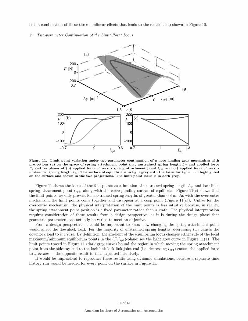
Figure 11. Limit point variation under two-parameter continuation of a nose landing gear mechanism withprojections (a) on the space of spring attachment point lsp1, unstrained spring length LU and applied forceF , and on planes of (b) applied force F versus spring attachment point lsp1 and (c) applied force F versusunstrained spring length LU . The surface of equilibria is in light grey with the locus for LU = 1.3m highlightedon the surface and shown in the two projections. The limit point locus is in dark grey.

Figure 11 shows the locus of the fold points as a function of unstrained spring length LU and lock-link-spring attachment point lsp1, along with the corresponding surface of equilibria. Figure 11(c) shows thatthe limit points are only present for unstrained spring lengths of greater than 0.8 m. As with the overcentremechanism, the limit points come together and disappear at a cusp point (Figure 11(c)). Unlike for theovercentre mechanism, the physical interpretation of the limit points is less intuitive because, in reality,the spring attachment point position is a fixed parameter rather than a state. The physical interpretationrequires consideration of these results from a design perspective, as it is during the design phase thatgeometric parameters can actually be varied to meet an objective.

From a design perspective, it could be important to know how changing the spring attachment pointwould affect the downlock load. For the majority of unstrained spring lengths, decreasing lsp1 causes thedownlock load to increase. By definition, the gradient of the equilibrium locus changes either side of the localmaximum/minimum equilibrium points in the (F, lsp1)-plane; see the light grey curve in Figure 11(a). Thelimit points traced in Figure 11 (dark grey curve) bound the region in which moving the spring attachmentpoint from the sidestay end to the lock-link-lock-link joint end (i.e. decreasing lsp1) causes the applied forceto decrease — the opposite result to that expected intuitively.

It would be impractical to reproduce these results using dynamic simulations, because a separate timehistory run would be needed for every point on the surface in Figure 11.

14 of 15

American Institute of Aeronautics and Astronautics

IV. Conclusion

It has been shown that continuation methods, when applied to mechanisms expressed as a set of staticequilibrium equations, provide steady-state solutions that are as accurate as traditional dynamic models.Solving static models in parameter space with a continuation algorithm offers significant reductions in com-putational times when compared to more traditional, dynamic simulation based approaches. This is becausesimpler models can be used and points of interest, such as the limit points, can be traced out directly undermultiple parameter variations. The results from the overcentre mechanism example show that it is alsopossible to follow unstable equilibria (determining boundaries of bistability) with continuation methods,something which cannot easily be achieved by dynamic simulations. The feasibility of this continuationapproach when applied to a complex mechanism became apparent from the nose landing gear mechanisminvestigation. The results for the nose landing gear model also demonstrate the flexibility of the analysisoffered by expressing the landing gear as a set of static equilibrium equations. It was shown that systemdependencies can be determined readily upon variation of any state or system parameter. This is a definiteadvantage over conventional dynamic simulations. For both the overcentre and nose landing gear mecha-nisms, examples were presented of how design criteria could potentially be derived from the continuationanalysis. The computational efficiency and flexibility achieved with the continuation approach makes ithighly suitable for analysing more complex three-dimensional mechanisms, such as a dual sidestay landinggear mechanism. For a dual sidestay landing gear, the mechanism can be described in terms of 36 geometricstates and 20 internal force states if using the static equation method. Besides the increase in model states,the nature of a dual sidestay landing gear mechanism is different from the nose landing gear mechanisminvestigated here because the dual sidestay is over-constrained, resulting in a highly sensitive downlock so-lution which only exists if all the downlock constraints are exactly satisfied. The continuation approachdescribed here would be well suited to investigating this highly nonlinear system in an efficient and thoroughmanner.

Acknowledgments

This research was supported by an Engineering and Physical Sciences Research Council (EPSRC) CaseAward grant in collaboration with Airbus in the UK.

References

1Lyle, K.H., Jackson, K.E., Fasanella, E.L., Simulation of Aircraft Landing Gears with a Nonlinear Dynamic FiniteElement Code, AIAA Journal of Aircraft, Vol. 39, No. 1, January – February 2002.

2Kruger, W., Besselink, I., Cowling, D., Doan, D.B., Kortum, W., Krabacher, W., Aircraft Landing Gear Dynamics:Simulation and Control, Vehicle System Dynamics, Vol. 28, 1997.

3Conway, H.G., Landing Gear Design. Chapman and Hall, London, 1958.4Currey, N.S., Aircraft Landing Gear Design: Principles and Practices. AIAA, Washington D.C, 1988.5Roskam, J., Airplane Design. Part 4, Layout design of landing gear and systems, Roskam Aviation and Engineering

Corporation, Ottawa, 1986.6Strogatz, S., Nonlinear dynamics and chaos, Springer, 2000.7Guckenheimer, J. and Holmes, P., Nonlinear Oscillations, Dynamical Systems and Bifurcations of Vector Fields, Applied

Mathematical Sciences Vol. 42, Westview Press, February 2002.8Krauskopf, B., Osinga, H. M., and Galan-Vioque, J., Numerical Continuation Methods for Dynamical Systems, Springer,

2007.9Rankin, J., Coetzee, E., Krauskopf, B. and Lowenberg, M., Bifurcation and Stability Analysis of Aircraft Turning on the

Ground, AIAA Journal of Guidance, Dynamics and Control, Vol. 32, No. 2, March 2009.10Thota, P., Krauskopf, B. and Lowenberg, M., Interaction of Torsion and Lateral Bending in Aircraft Nose Landing Gear

Shimmy, Nonlinear Dynamics, 57(3), 2009.11Doedel, E., Champneys, A., Fairgrieve, T., Kuznetsov, Y., Sandstede, B., and Wang, X., AUTO 97 : Continuation and

bifurcation software for ordinary differential equations, http://indy.cs.concordia.ca/auto/, May 2001.12Udwadia, F.E. and Kalaba, R.E., Analytical Dynamics: A New Approach. Cambridge University Press, New York, 1996.

15 of 15

American Institute of Aeronautics and Astronautics