Page 1
Numerical investigation of the Sicily Channel dynamics:
density currents and water mass advection
Anne Molcard a,b,*, Liliana Gervasio a, Annalisa Griffa a,b, Gian Pietro Gasparini a,Laurent Mortier c, Tamay M. Ozgokmen b
aIOF-CNR, La Spezia, ItalybRSMAS/MPO, University of Miami, Miami, FL, USA
cLODYC-CNRS/ENSTA, Paris, France
Received 20 June 2001; accepted 29 May 2002
Abstract
The Sicily Channel connects the western and eastern Mediterranean sub-basins, playing a fundamental role in the dynamics
of the Mediterranean circulation. The flow in the Channel is driven by direct forcing such as wind and by thermohaline
processes leading to density difference between the two sub-basins. Assessing the relative role of these two types of forcing
mechanisms is still an open question in the literature, despite its importance for a correct understanding and prediction of the
Channel circulation. In this paper, we isolate the remotely forced, density-driven component of the circulation, considering a
simplified setting, where the forcing is schematized as an imposed density difference along the channel, Dq. The study is carriedout considering results from a high resolution numerical model of the circulation in the Channel area. A range of values for Dqis considered, and the effects of changing Dq on the circulation patterns, transport values and water mass advection are studied.
The patterns of the average circulation and water mass advection remain qualitatively similar at varying Dq. The simulations
reproduce a number of realistic circulation features for both the surface Modified Atlantic Water (MAW) and the Levantine
Intermediate Water (LIW). These include the complex branching patterns of the MAW at the entrance of the Channel, and the
appearance of the characteristic structure of the Atlantic Ionian Stream (AIS) inside the Channel. At a more detailed level, the
nonlinearity at increasing Dq appears to influence some aspects of the circulation, such as the relative strength of the Tyrrhenian
and Sicilian MAW branches.
The transport across the Channel is found to increase approximately linearly with Dq in the considered range, with values
ranging from c 0.3 to c 0.8 Sv. The lowest value corresponds to Dq based on climatological density value in the
neighbouring regions (Sardinia Channel and Ionian Sea), while the highest values correspond to more remote density values,
i.e. to differences between the far-field western and eastern Mediterranean sub-basins.
D 2002 Elsevier Science B.V. All rights reserved.
Keywords: Water balance; Current; Numerical model; Sicily Strait
0924-7963/02/$ - see front matter D 2002 Elsevier Science B.V. All rights reserved.
PII: S0924 -7963 (02 )00188 -4
* Corresponding author. IOF-CNR, Forte Santa Teresa, 19036 Pozzuolo di Lerici (SP), Italy. Tel.: +39-0187-978302; fax: +39-0187-
970585.
E-mail address: [email protected] (A. Molcard).
www.elsevier.com/locate/jmarsys
Journal of Marine Systems 36 (2002) 219–238
Page 2
1. Introduction
The Sicily Channel connects the Eastern and West-
ern Mediterranean Sea, playing an important role in
the dynamics of the Mediterranean general circula-
tion. At first approximation, the flow through the
Sicily Channel can be considered as a two-layer
system, in which the surface water of Atlantic origin,
characterized by minimum salinity (Modified Atlantic
Water, MAW), flows eastward, and the Levantine
Intermediate Water (LIW), characterized by maximum
salinity, flows westward underneath. Basic knowledge
on the main current patterns is provided by observa-
tions (e.g. Astraldi et al., 1996, 1999; Malanotte-
Rizzoli et al., 1997; Manzella et al., 1988, 1990;
Moretti et al., 1993; Robinson et al., 1999; Sparnoc-
chia et al., 1999), even though less numerous than in
the other main strait of the Mediterranean Sea, namely
the Gibraltar Strait (e.g. see Pratt, 1990 for a review).
A schematic illustration of the circulation and of the
water mass pathways, as indicated by the measure-
ments in this region is shown in Fig. 1.
The MAW (Fig. 1a) flows from the Western
Mediterranean along the Algerian coast and bifurcates
at the Channel level: one branch, carrying about 1/3 of
the incoming transport, crosses the Channel and con-
tinues eastward in the Tyrrhenian Sea along the north-
ern coast of Sicily, while the other branch, carrying
approximately 2/3 of the transport, enters into the
Channel. The path of the latter is variable in time, and
this branch is possibly subject to additional branching.
Signatures of minimum salinity are found close to the
Tunisian coast at the entrance of the Channel (Astraldi
et al., 1996). The subsequent path is not known
exactly because direct measurements are not available
on the southern Tunisian shelf. The MAW is also
found entering the Channel along the Sicilian coast
and in the center of the Channel, which suggests the
presence of a secondary branching (shown by the
dashed line in Fig. 1a). Independently from the exact
entrance point, a consistent vein of the MAW, often
indicated as the Atlantic Ionian Stream (AIS), appears
to reach the Sicilian shelf north of Malta, subse-
quently following the shelf and reaching the Ionian
Sea. Robinson et al. (1999) underline the presence of
some permanent structures in the path of the AIS.
The LIW (Fig. 1b) enters the Channel from the
adjacent Ionian Sea, from the eastern side. Even
though the LIW occupies most of the Channel below
a depth of 200 m, its main salinity core is observed to
lay close to the Sicilian shelf, suggesting a position for
the main current. The LIW flows out of the Channel
over two main sills in the western side. After that, it
appears to flow mostly eastward following the Tyr-
rhenian coast (Astraldi et al., 1996).
The mass flux crossing the Channel is estimated
from observations to have a mean value on the order
of 1 Sv, but with a high variability. Geostrophic
Fig. 1. The study area with the model bathymetry and the schematic
pathways of (a) the MAW and (b) the LIW.
A. Molcard et al. / Journal of Marine Systems 36 (2002) 219–238220
Page 3
computations using hydrographic transects crossing
the Channel yield values ranging from 1.15–1.23 Sv
(Garzoli and Maillard, 1979) to 0.37–0.41 Sv (Mor-
etti et al., 1993). Long-term current measurements
indicate a mean transport of 1.1 Sv during the period
1993–1997 with a standard deviation of 0.58 Sv
(Astraldi et al., 1999).
Dynamical forcing mechanisms in the Channel
include both local atmospheric forcings such as wind
and buoyancy fluxes and also remote forcing, mostly
related to thermohaline processes leading to density
differences between the western and eastern Mediter-
ranean sub-basins. Assessing the relative role of these
two types of forcing mechanisms is still an open
question in the literature, despite its importance for a
correct understanding and prediction of the Channel
circulation. Results from direct observations (e.g.
Astraldi et al., 1999) and from general circulation
models (e.g. Horton et al., 1997; Korres et al., 2000)
provide information on the overall characteristics of
the circulation, but they cannot be used directly to
separate the effects of various forcing mechanisms.
Considerations based on salt and mass conservation
suggest the relevance of the thermohaline remote
forcing, yielding a thermohaline transport in the Strait
of approximately 1 Sv (Bethoux, 1979; Hopkins,
1999), while model results tend to indicate the rele-
vance of the wind stress in determining the flux values
(Heburn, 1994; Korres et al., 2000). Regional model-
ing studies (Onken and Sellshop, 1998; Pierini and
Rubino, 2001) do not provide a direct insight on the
nature of the forcing, since they investigate the onset
of circulation and instabilities for specified values of
incoming fluxes.
The objective in this study is to investigate how
much of the circulation patterns in the Sicily Channel
region can be captured by using an idealized, local
model with thermohaline forcing only. A simplified
setting is considered, where the forcing is schematized
as a boundary forcing, characterized by an imposed
density difference along the channel, Dq. Using this
simple model, we address the following questions:
can thermohaline forcing alone generate anything like
what is seen in the observations, or something quite
different? If it generates circulation patterns resem-
bling those from observations, how much forcing at
the boundaries is needed to do so? How do the interior
patterns and the transport through the Channel vary as
a function of the boundary forcing? What is the
reasonable range of boundary forcing, or equivalently
of Dq, required to induce the observed level of
Channel transport? Which observed circulation pat-
terns cannot be captured and cannot be explained
using boundary thermohaline forcing only? It will
be therefore deduced indirectly which circulation
patterns require other forcing mechanisms, such as
wind forcing and the use of more sophisticated
models.
A process study is performed varying the strength
of the forcing and studying the response of the system
through numerical integration of a high resolution
circulation model of the Channel area, with realistic
topography. A similar approach has been previously
followed in other papers (Herbaut et al., 1996, 1998;
Gervasio et al., submitted for publication), focusing
on analytical and numerical spin-up solutions of
simplified models. Here we consider the longer time
evolution of the system, with special interest in trans-
port and water mass properties.
Results from three main numerical experiments are
presented in detail. They focus on the effects of
surface density difference across the Channel, and
cover a realistic range of climatological Dq values.
The effects of changing Dq on the circulation patterns,
water mass advection and transport values are studied.
A comparison is performed between transport values
obtained from the circulation model, and bulk esti-
mates obtained using the simplified steric height
methods (Hopkins, 1999). The method is also used
to investigate the effects of the (smaller) density
difference occurring in the intermediate layer.
The paper is organized as follows. In Section 2, the
numerical model and the configuration of the experi-
ments are discussed, while the results are presented in
Section 3. In Section 4, the comparison with the
results using the steric height method is shown. A
summary of this study and conclusions are provided
in Section 5.
2. Numerical model, configuration and forcing
representation
Numerical experiments are performed using OPA7
(Ocean Parallel), a finite difference primitive equation
model originally developed at Lodyc. The model is
A. Molcard et al. / Journal of Marine Systems 36 (2002) 219–238 221
Page 4
well documented in the literature, and the reader is
referred to Andrich et al. (1988) and Madec et al.
(1991a,b) for a review of the details of this model. The
version utilized in the present study is subject to rigid-
lid and hydrostatic approximations, and employs a z-
coordinate system for vertical discretization. Subgrid-
scale physics is parameterized by a fourth-order
operator for momentum and tracers. The horizontal
eddy viscosity and diffusion coefficients are equal to
109 m4 s� 1 (as we use a bi-Laplacian operator) and
the vertical coefficients are assumed to vary as a
function of the local Richardson number according
to the parameterization proposed by Pacanowski and
Philander (1981).
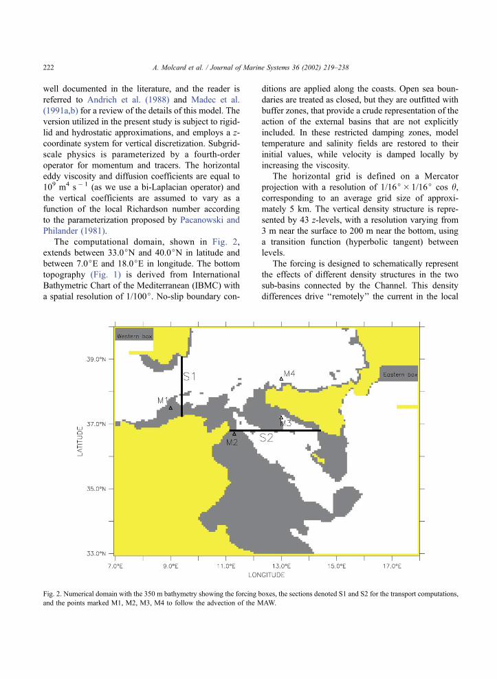
The computational domain, shown in Fig. 2,
extends between 33.0jN and 40.0jN in latitude and
between 7.0jE and 18.0jE in longitude. The bottom
topography (Fig. 1) is derived from International
Bathymetric Chart of the Mediterranean (IBMC) with
a spatial resolution of 1/100j. No-slip boundary con-
ditions are applied along the coasts. Open sea boun-
daries are treated as closed, but they are outfitted with
buffer zones, that provide a crude representation of the
action of the external basins that are not explicitly
included. In these restricted damping zones, model
temperature and salinity fields are restored to their
initial values, while velocity is damped locally by
increasing the viscosity.
The horizontal grid is defined on a Mercator
projection with a resolution of 1/16j� 1/16j cos h,corresponding to an average grid size of approxi-
mately 5 km. The vertical density structure is repre-
sented by 43 z-levels, with a resolution varying from
3 m near the surface to 200 m near the bottom, using
a transition function (hyperbolic tangent) between
levels.
The forcing is designed to schematically represent
the effects of different density structures in the two
sub-basins connected by the Channel. This density
differences drive ‘‘remotely’’ the current in the local
Fig. 2. Numerical domain with the 350 m bathymetry showing the forcing boxes, the sections denoted S1 and S2 for the transport computations,
and the points marked M1, M2, M3, M4 to follow the advection of the MAW.
A. Molcard et al. / Journal of Marine Systems 36 (2002) 219–238222
Page 5
Channel area, through the propagation of the so-called
Kelvin fronts (e.g. Herbaut et al., 1998). In a number
of previous papers, (e.g. Herbaut et al., 1996, 1998;
Gervasio et al., submitted for publication), this remote
forcing has been studied using a simplified setting
where the sub-basins are schematically represented by
‘‘boxes’’, where the density profiles and the associated
gradients with ambient waters are maintained con-
stant. Conceptually, these boxes represent the reser-
voir of available potential energy contained in the sub-
basins and act as ‘‘motor’’ for the system. The same
framework is used in the present paper.
In the numerical experiments presented in Section
3, the forcing boxes are situated as shown in Fig. 2.
The western box is located in the northwestern
corner of the domain near Sardinia, and it character-
izes the inflowing MAW with relatively low density.
The eastern box is situated in the northeast region, in
the denser Ionian Sea, and characterizes the AIS
outflowing from the basin. In preliminary experi-
ments, the sensitivity to the specific box location and
size has been studied. In particular, the latitudinal
extent of the eastern box has been modified, up to
cover the whole eastern boundary. The results in
terms of circulation and transport in the Channel are
found to be quite insensitive (see Section 3.1 for
details).
The density profiles in the boxes are idealized to
characterize a three-layer system (Table 1). Three
main experiments are considered, DG1, DG2, DG3.
They focus on the surface density difference (approx-
imately upper 150 m), which is more than an order of
magnitude bigger than the differences in the lower
levels (see Section 4). The densities of the intermedi-
ate and deep layers are assumed to be the same in the
three experiments as well as in the two boxes and in
the initial basin stratification. In this setting, then, the
forcing is provided by the surface gradient which
determines a baroclinic current with a surface compo-
nent representing the MAW and an intermediate
component representing the LIW. This choice of the
forcing is of course a crude simplification of reality,
but it allows to isolate the effects of the main forcing
function. The effects of intermediate density differ-
ences is investigated using the steric height method in
Section 4.
The three runs are characterized by increasing
surface density difference between the two boxes,
Dq = 0.77, 1.53, 2.30 for DG1, DG2 and DG3,
respectively (Table 2), corresponding to a factor of 2
between DG1 and DG2 and to a factor 3 between
DG1 and DG3. The lowest Dq (DG1) corresponds to
differences between climatological density (Brasseur
et al., 1996; Guibout, 1987) in the neighbouring
regions (Sardinia Channel and Ionian Sea), while the
highest Dq (DG3) corresponds to differences between
the far-field western and eastern Mediterranean
(approximately corresponding to the Alboran Sea
and the Levantine basin). An intermediate Dq value
is chosen for DG2.
The density profiles defined in the two boxes are
maintained throughout the integrations, as well as
Table 1
Densities values in the surface, intermediate and bottom layers for
experiments DG1, DG2 and DG3
Box1 Interior Box2
DG1
27.19 27.57 27.96
29.07 29.07 29.07
29.09 29.09 29.09
DG2
26.81 27.57 28.34
29.07 29.07 29.07
29.09 29.09 29.09
DG3
26.42 27.57 28.72
29.07 29.07 29.07
29.09 29.09 29.09
The ‘‘box’’ densities are kept fixed, whereas the ‘‘interior’’ density
corresponds to that at the initial time. The thicknesses of the surface,
intermediate and bottom layers are 150, 450, and 3500 m,
respectively.
Table 2
Values of density differences between the two boxes, Dq, volume
transports in Sv (meanF standard deviation) across sections S1 and
S2 (see Fig. 2) and their ratios (multiplied by 3), for experiments
DG1, DG2 and DG3
DG1 DG2 DG3
Dq 0.77 1.53 2.30
S1 0.47F 12% 0.92F 21% 1.39F 15%
S2 0.31F17% 0.53F 21% 0.810F 19%
S3 0.16 0.39 0.58
3� S3/S1 1.02 1.27 1.25
3� S2/S1 1.98 1.73 1.75
A. Molcard et al. / Journal of Marine Systems 36 (2002) 219–238 223
Page 6
their gradients with the ambient waters, by constant
linear relaxation of the corresponding temperature and
salinity profiles toward the initial values (using a
relaxation coefficient of 1 day). In all the three runs,
the rest of the domain is initialized with a surface
Mediterranean density corresponding to the average
of the two box values to guarantee that the density
gradient is the same for the two boxes. This ‘‘central
Mediterranean’’ density profile is let free to evolve
according to the model dynamics. The time step used
in the numerical integration ranges from 14 min for
experiments DG1 and DG2, to 7 min for DG3.
3. Results from numerical experiments
In the following, the results of the three experi-
ments DG1, DG2 and DG3 are presented. First, the
basic mechanisms of the first spin-up phase are briefly
reviewed. Then, the characteristics of the solutions are
illustrated with emphasis on the general circulation
patterns, water-mass advection characteristics and
transports at selected sections. Notice that the first
spin-up phase (Section 3.1) is not realistic, since it
depends on the artificial initial condition. Neverthe-
less, as shown in a number of previous papers, (e.g.
Herbaut et al., 1996, 1998; Pierini and Rubino, 2001),
this phase can be of interest because it provides some
understanding of the circulation setting and it allows
to isolate and separetely study the role of the various
boundary forcings. Also, the results are relevant to the
understanding of transients due to time dependent
perturbations of the forcings, such as for periods
following intense dense-water formation elsewhere
in the Mediterranean basin.
3.1. First spin-up phase
The first phase of the spin-up is very similar for all
three experiments, and is dominated by the set-up of
coastal currents generated by incident Kelvin fronts
due to density gradients (Speich et al., 1996). At the
initial time, in fact, the ‘‘gates’’ of the two boxes (Fig.
2) are opened, and a current system is set up by the
density gradients. For the configuration in Fig. 2, the
solution is expected to be due to the superposition of
two Kelvin fronts, generated by the western and
eastern box, respectively. In order to illustrate the role
of each box, we have first performed a preliminary
experiment considering the action of each box separ-
etely. The results are shown in Fig. 3 for DG3.
The gradient in the western box, where surface
water is lighter, generates a Kelvin front flowing
eastward along the Tunisian coast and sets an east-
ward surface current (Fig. 3a). At the Channel
entrance (Herbaut et al., 1998), a barotropic and
baroclinic double Kelvin wave associated to the shelf
break north of the Channel causes the front to sepa-
rate, generating two main surface current branches.
One branch enters the Channel and flows south along
the Tunisian coast, whereas the other branch crosses
the Channel and reaches the Tyrrhenian Sea.
The front induced by the eastern box, instead, is
characterized by denser surface water. It propagates
along the Sicilian coast (Gervasio et al., submitted for
publication), keeping the coast to its right, while
generating a surface coastal current moving in the
opposite direction, i.e. southeastward in the Channel
toward the box (Fig. 3b). This current connects the
Tyrrhenian and the Ionian Sea, flowing along the
Sicily coast through the Channel and then northward
in the Ionian Sea.
When both boxes are active, the two fronts and the
associated currents joint to set up the basin circulation
(Fig. 4c). The current pattern shows the main MAW
bifurcations and the typical pattern of the AIS. Notice
that the solution in Fig. 4c corresponds almost exactly
to the linear superposition of the two solutions in Fig.
3a,b, indicating that the dynamics in this phase is in
good approximation linear. This is shown also by the
striking resemblance of the flow patterns for the
various experiments (see Fig. 4a for DG1), after the
same integration time. The preliminary experiments
indicate that the MAW branching and the setting of
the Tunisian current are mostly related to density
differences with the western basin, while the north-
ward current in the Ionian sea and the AIS pattern are
mostly due to differences with the eastern basin.
The time scale of this first spin-up phase is related
to the time necessary for the Kelvin front to circulate
around the basin. This phase speed depends primarily
on the vertical initial basin stratification (Herbaut et
al., 1998), which is the same for all the experiments,
and it is on the order of 1 m s� 1. The spin-up phase,
then, is expected to last less than 20 days, as con-
firmed by the numerical results. The current patterns
A. Molcard et al. / Journal of Marine Systems 36 (2002) 219–238224
Page 7
in Figs. 3 and 4a–c, in fact, are obtained at t= 15
days.
It is interesting to note that results analogous to
those in Fig. 3 are obtained also when the box shape is
changed, for example increasing the latitudinal extent
of the eastern box (as already mentioned in Section 2).
Results at t= 15 days for an eastern box covering the
whole eastern boundary are shown in Fig. 3c. The
circulation ouside from the box is equivalent to the
circulation in Fig. 4c, and also the transport values
across the Strait are the same. Similar results have also
been reported by Pierini and Rubino (2001), using a
different model setting. In Pierini and Rubino (2001),
the circulation in the Sicily Channel is forced by
prescribed transports uniformely distributed along
two prescribed sections at the two opposite sides of
the Channel. The spin-up circulation is dominated by
Kelvin fronts propagating along the coasts and leads
to localized currents, which are very similar to those
in Fig. 4a–c. This indicates generality of the results
with respect to specific configurations.
3.2. Subsequent evolution and time-averaged velocity
fields
After the first spin-up phase, the solution enters a
second phase of evolution dominated by the advection
of the low density MAW in the basin. The time scale
of this phase is related to current advection, and it is
expected to be significantly longer since the advection
velocity is significantly smaller than the Kelvin front
phase speed. The results relative to the circulation in
this phase are shown here for the three experiments,
starting from DG1, characterized by the lowest den-
sity difference Dq (Table 1).
The DG1 experiment is integrated for a total time
of 3.5 years. A first characterization is given by the
evolution of the density integrated over the whole
basin in the upper layer, where the MAW is advected:
qDðtÞ ¼
ZA
dxdy
Z �D
0
dzqðx; y; z; tÞZA
dxdy
Z �D
0
dz
: ð1Þ
In Eq. (1), A is the horizontal basin domain, z = 0 is
the surface level and D is a prescribed depth of
integration in the upper layer. Results showing the
Fig. 3. Snapshots of surface velocity (in m s� 1) for experiment
DG3 at 15 days with (a) only the western box, (b) only the eastern
box and (c) with the western box and an eastern box covering the
whole eastern boundary.
A. Molcard et al. / Journal of Marine Systems 36 (2002) 219–238 225
Page 8
evolution of qD(t) for D = 15 m, i.e. for shallow
integration, are shown in Fig. 5a. Similar results are
found for D up to approximately 55 m. For D>55 m,
oscillations start to occur due to the motion of the
interface between different water masses (Table 1).
The behavior of qD (Fig. 5a) indicates that the
simulation has not yet reached a complete equilibrium
at the end of the integration period of 3.5 years. The
most noticeable changes, though, occur during the
first 2 years, as shown also by the MAW advection
patterns discussed in Section 3.3.
During this phase of evolution, the instantaneous
surface circulation changes significantly from the
initial spin-up phase (Fig. 4a), developing instabil-
ities and a vigorous mesoscale eddy field. An exam-
ple of the instantaneous flow field during this fully
developed phase is shown in Fig. 4b, after approx-
imately 6 months of integration. Time averages of
the circulation, on the other hand (computed every 3
and 6 months), do not show significant changes after
the first 3 months, maintaining a quasi-stationary
pattern.
The surface average velocity in experiment DG1 is
shown in Fig. 6a. The MAW flows eastward from the
western box, roughly following the topography along
the Tunisian shelf. At the Channel level, branching of
Fig. 4. Snapshots of surface velocity (in m s� 1) for (a) the experiment DG1 at 15 days (b) the experiment DG1 at 6 months, (c) the experiment
DG3 at 15 days, and (d) the experiment DG3 at 6 months.
A. Molcard et al. / Journal of Marine Systems 36 (2002) 219–238226
Page 9
the flow takes place, similarly to that shown in the
spin-up solution (Fig. 4a). One branch crosses the
Channel and continues eastward in the Tyrrhenian Sea
along the northern coast of Sicily, while two other
branches enter the Channel, the main branch flowing
southward along the Tunisian coast and a secondary
branch along the western coast of Sicily. The Tunisian
branch appears to later cross the Channel to join the
Sicily coast north of Malta. The joint current then
flows northward in the Ionian Sea following the coast.
The structure of the simulated velocity field is
qualitatively similar to the observed AIS pattern
(Fig. 1a). The magnitudes of velocities, however, are
significantly lower than the observations, approxi-
mately by a factor of 3.
Next, the effect of increasing the density difference
Dq on the circulation patterns is studied by consider-
ing the results from experiments DG2 and DG3. The
experiments DG2 and DG3 are integrated for a shorter
time than the experiment DG1, for 6 and 8 months,
respectively. This is partially justified by the fact that
the time evolution in these experiments is expected to
be faster, since the advection velocity scales are larger
for DG2 and DG3 than for DG1. A bulk estimate of
the change in advection velocity as function of Dq is
provided by the transport values in the three experi-
ments (see Section 3.4 and Table 2). They suggest a
roughly linear increase of advection velocity with Dq,with a factor c 2 and 3 with respect to DG1 for DG2
and DG3, respectively. If the time scale of evolution is
Fig. 5. Time evolution of basin-integrated density qD(t) calculated for D= 15 m (a) for the experiment DG1 and (b) for the experiment DG3.
A. Molcard et al. / Journal of Marine Systems 36 (2002) 219–238 227
Page 10
assumed to be inversely proportional to the advection
velocity scale, this suggests 2 (3) times shorter time
scales for DG2 (DG3) with respect to DG1. This is in
qualitative agreement with the time evolution of qD(t)
(defined in Eq. (1)) for DG3 (Fig. 5): qD(t) in DG3
has a similar behaviour to that from DG1, but with a
time scale approximately 3 times faster (analogous
results are obtained for DG2, with a corresponding
factor of 2).
During this phase, the instantaneous velocity field
in DG3 (and DG2) is unstable as in DG1, as illustrated
by the snapshot at t = 6 months in Fig. 4d. Also as in
DG1, the time averages of the velocity field do not
change significantly (after the first month period),
suggesting that the velocity statistics is quasi-station-
ary even though the density field is still evolving. Fig.
6b,c show the average velocity fields for DG2 and
DG3 performed over the whole integration period,
starting at t = 1 month.
The surface velocity structure (Fig. 6a–c) is qual-
itatively similar in the three experiments, showing
similar branching at the Channel entrance and the
characteristic AIS pattern. At a more detailed level,
though, differences can be noticed, especially regard-
ing the southward Sicilian current. The relative
strength of this current appears to intensify at increas-
ing Dq, i.e. at increasing nonlinearity. One possible
explanation for this behavior is that the incoming
MAW tends to mix more vigorously and rapidly at
increasing nonlinearity, and this leads to a decrease in
the associated density gradient. As shown in Section
3.1, the MAW density gradient is primarily associated
with the branching and setting of the Tunisian south-
ward current. As a consequence, the decrease in the
MAW gradient results in a weakening of the Tunisian
current and a relative strengthening of the Sicilian
current.
Time-averaged circulation patterns at the inter-
mediate level (350 m) are depicted in Fig. 7. In
DG1, the velocity field at this level (Fig. 7a) is found
to have a structure qualitatively similar to the
observed pattern (Fig. 1b), but the velocity values
are smaller, as for the surface circulation. The main
current enters the Channel through the eastern sill,
close to the Sicilian shelf, flowing toward the north-
west. After exiting the western side of the Channel,
the current flows mostly eastward following the Tyr-
rhenian shelf. This circulation pattern is similar in the
three experiments, suggesting a weaker dependence
on nonlinearity with respect to the surface velocity.
This is not surprising given the stronger topographic
constraint, especially inside the Channel area. The
most noticeable difference between the experiments
Fig. 6. Time-averaged surface circulation (in m s� 1) for the
experiments (a) DG1 (averaged over 2 years), (b) DG2 (averaged
over 6 months) and (c) DG3 (averaged over 8 months).
A. Molcard et al. / Journal of Marine Systems 36 (2002) 219–238228
Page 11
takes place outside the Channel, in the eastward
Tyrrhenian current, which becomes stronger with
increasing Dq (Fig. 7a–c) in a consistent manner with
the increased Tyrrhenian transport discussed above.
A qualitative validation of the model can be
obtained comparing model and in-situ observations
of property distribution. In Fig. 8, the salinity S
distribution at a section across the Channel from the
experiment DG1 at t = 3.5 years is compared to that
from in-situ data. While the realistic salinity values
are not reproduced in the model simulation, since the
solution is not yet at equilibrium and still depends on
the choice of the initial values (especially for the LIW,
see Table 3), the spatial structure of the isolines
appears to be in good agreement with that from
observations. The vertical and horizontal structure of
the two main water masses (MAW at the surface and
LIW at intermediate level), and their core positions are
satisfactorily reproduced by the model. The S mini-
mum occurs in the surface level. Its core (indicative of
the MAW) is found near to the Tunisian coast, and it
weakens toward the sicilian coast. Maximum salinity
values, instead, are indicative of the presence of LIW
water and are found in the intermediate level. LIW
water is found predominantly in the eastern part of the
basin, closer to the sicilian coast. The similarity
between S patterns in model and data suggests that
also the underlying velocity structure of the model is
realistic. Whether the model is capable of reproducing
realistic features because of its internal model dynam-
ics or because of the constraints imposed by the
boundary conditions is a question that cannot be
answered at this point, as for any regional model.
3.3. Water mass advection
The advection of the MAW is first studied qual-
itatively following the spreading in time of its signa-
ture in terms of lighter density water. Density maps at
3-month intervals from the beginning of the experi-
ment DG1 are shown in Fig. 9, providing a direct
visualization of the main paths of advection. At t= 3
months (Fig. 9a), the MAW reaches the Channel,
while by t = 6 months (Fig. 9b), the branching in the
velocity field clearly influences the density distribu-
tion. Two main low-density branches are evident, one
entering the Channel along the Tunisian shelf and the
other crossing the Channel into the Tyrrhenian Sea.
There is also an indication of a third branch flowing in
the Channel following the western Sicilian coast. In
the following months (Fig. 9c), a progressive south-
westward motion of the MAW is observed in the
Channel, developing patterns similar to the observed
AIS (Robinson et al., 1999; Malanotte-Rizzoli et al.,
Fig. 7. Time-averaged intermediate level (350 m) circulation (in
m s� 1) for the experiments (a) DG1, (b) DG2 and (c) DG3.
A. Molcard et al. / Journal of Marine Systems 36 (2002) 219–238 229
Page 12
Fig. 8. Salinity distributions (in psu) at a section across the Sicily Channel from in-situ data (MATER2 Cruise, January 1997) and from the
experiment DG1.
A. Molcard et al. / Journal of Marine Systems 36 (2002) 219–238230
Page 13
1997). At t = 1 year (Fig. 9d), the MAW reaches the
Ionian Sea (corresponding to the significant decrease
of the slope of qD in Fig. 5). After 2 years of
integration (not shown) the MAW reaches the eastern
wall, where the buffer zones maintain the density
gradient.
As a next step, some more detailed and quantitative
questions are considered about MAW advection.
Observations (Sparnocchia et al., 1999; Astraldi et
al., 1996) show that at the entrance of the Channel,
minimum density values are found close to Tunisia.
This suggests that the Tunisian branch is the most
effective one in transporting the MAW, while the role
of the current along the Sicily coast in advecting
MAW it is not entirely clear.
In order to explore these issues using the model
results and in order to obtain a more quantitative
picture of MAW advection, the time series of q(t) atfour different points in the domain are computed.
Notice that model results, strictly speaking, cannot
be directly compared to observation, since the solu-
tion is still evolving and the results cannot be consid-
ered as representative of ‘‘typical’’ MAW pathways.
Fig. 9. Snapshots of surface density (r= q� 1000 in kg m� 3) in the experiment DG1 at (a) 3, (b) 6, (c) 9 and (d) 12 months.
Table 3
Salinity values in the surface, intermediate and bottom layers for
experiment DG1
Box1 Interior Box2
37.5 38 38.5
38.5 38.5 39
38.75 38.75 38.75
The ‘‘box’’ salinities are kept fixed, whereas the ‘‘interior’’ salinity
corresponds to that at the initial time. The thicknesses of the surface,
intermediate and bottom layers are 150, 450, and 3500 m,
respectively.
A. Molcard et al. / Journal of Marine Systems 36 (2002) 219–238 231
Page 14
Nevertheless, the spin up process is useful to under-
stand the mechanisms of advection and mixing, and it
can be used to understand tendencies in the solution.
The four points of measurements, M1, M2, M3, M4,
are indicated in Fig. 2. The point M1 is located north
of the Tunisian coast, outside from the Channel. The
points M2 and M3 are inside the Channel, close to the
Tunisian and Sicilian coasts, respectively, while the
point M4 is located in the Tyrrhenian Sea. In all cases,
the density q(t) is computed at the surface level, where
the low density signal is more evident.
The results from experiment DG1 (Fig. 10a) show
that the highest and most stable signal of the MAW
advection is present at point M1. This is expected
since M1 is the closest point to the source and it is
located upstream of the Channel bifurcations. The
effect of the incoming MAW starts after 2 months
of integration and reaches an equilibrium value (den-
sity minimum) after approximately 1 year. This value
is approximately the average between the initial value
and the density value of the water from the Atlantic
box (see Table 1). For the other points, greater
variability in the evolution of density is present,
probably due to higher mesoscale variability. Despite
this, a clear arrival signal for the MAW can be noticed
at all points, characterized by a sharp decrease of q(t).
Fig. 10. Evolution of density (r= q� 1000 in kg m3) in time at the locations M1, M2, M3, M4 (see Fig. 2) in the experiments (a) DG1 and (b)
DG3.
A. Molcard et al. / Journal of Marine Systems 36 (2002) 219–238232
Page 15
The first point reached by the MAW after M1 is M2
(at tc 3 months), where also the lowest density value
at equilibrium is found. This indicates that the main
incoming path of the MAW into the Channel is indeed
along the Tunisian coast. Next arrival times occur at
M4 (at tc 4 months) and then at M3(at tc 6
months). The density values in the two points are
qualitatively similar (aside from strong fluctuations at
M4), and they are distinctively higher than those at
M2. This suggest that while the MAW advection is
confirmed at both points, the density signal is weaker
because of more extensive mixing. Also, it is possible
that the water advected in the Channel along the
Sicilian coast is partially recirculating in the Tyrrhe-
nian Sea before entering the Channel, as suggested by
the later arrival and similar mixing.
The results in regards to the advection of MAW
using the surface density evolution q(t) at the points
M1–M4 from the experiment DG3 are shown Fig.
10b. As in the experiment DG1, the fastest and
clearest signal of the MAW advection is found at
point M1 (at tc 15 days), and a few days later at M2.
The equilibrium value of the density at these points is
r = q� 1000c 27.2. Note that the density is rela-
tively higher than the average between the initial
condition value and the value of the incoming Atlantic
water, suggesting a more vigorous mixing close to the
box, as discussed above. As in DG1, the density at
points M3 and M4 are very similar and higher than
that at point M2.
Similar results are found in the experiment DG2
(not shown) to those in DG1 and DG3, confirming
that the incoming MAW is advected in the Channel
and splits into three main branches and that the
stronger signal is always present in the branch along
the Tunisian coast.
3.4. Transport
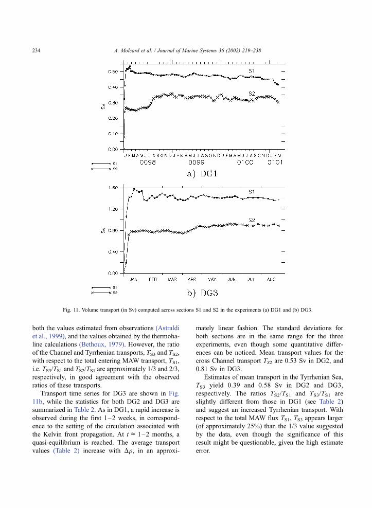
Transport time series of the surface MAW (Fig. 11)
are computed across the two vertical closed sections
shown in Fig. 2: Section S1 is across the Sardinia
Channel between Tunisia and Sardinia, and Section
S2 is across the Sicily Channel between Tunisia and
Sicily. Transport across S1, denoted TS1, characterizes
the MAW mass flux entering the domain, while
transport across S2, TS2, quantifies the mass flux
across the Channel. Using TS1 and TS2, an estimate
can be obtained also for the transport entering the
Tyrrhenian Sea, TS3 = TS1� TS2, which is not esti-
mated directly because the section cannot be closed
correctly at the northern boundary of the domain,
which is artificially closed by a buffer zone charac-
terized by a weak return flow (see Fig. 4). Note that,
due to the rigid-lid assumption, the net volume trans-
port across the Channel, integrated over the whole
water column, has to be zero at all times. Conse-
quently, the transport in the two layers (MAW and
LIW) is equal and opposite.
The transport calculation is done according to the
definition
T ¼ZL
dl
Z �DV
0
dzvn ð2Þ
where L is the section, n is the unit vector normal to
the section, v is the horizontal velocity vector and DV
is the depth at which vn changes sign in average.
The results for the time series TS1 and TS2 from the
experiment DG1 are shown in Fig. 11a and are
summarized in Table 2 in terms of mean and standard
deviation (s.d.). The parameter DV in Eq. (2) has been
chosen by analyzing isopycnals and velocity distribu-
tions in the vertical sections, in order to obtain an
estimate of the averge interface depth. Sensitivity to
the DV values has been tested over a wide range, and
this parameter was chosen in order to obtain the
highest and most stable transport across a specific
section (as the MAW structure can change depth
during its route). The values of this parameter are
taken as DV= 200 m for TS1 and DV= 150 m for TS2.
As can be seen in Fig. 11a and Table 2, the time series
becomes quite regular after the first adjustment phase
of approximately 1 month, with s.d. on the order of
12–21% with respect to the mean. Strictly speaking,
since the solution is still evolving, the mean transport
values cannot be considered as definitive and signifi-
cant of the equilibrium solution. On the other hand,
given the absence of obvious trends, we can assume
that they can be used to at least provide qualitative
estimates of the transport properties in the area.
The mean transport values in experiment DG1 are
0.47 Sv for TS1, and 0.31 Sv for TS2, suggesting a
Tyrrhenian Sea transport TS3 of c 0.16 Sv. The
transport TS2 across the Sicily Channel appears sig-
nificantly smaller (of approximately a factor 1/3) than
A. Molcard et al. / Journal of Marine Systems 36 (2002) 219–238 233
Page 16
both the values estimated from observations (Astraldi
et al., 1999), and the values obtained by the thermoha-
line calculations (Bethoux, 1979). However, the ratio
of the Channel and Tyrrhenian transports, TS3 and TS2,
with respect to the total entering MAW transport, TS1,
i.e. TS3/TS1 and TS2/TS1 are approximately 1/3 and 2/3,
respectively, in good agreement with the observed
ratios of these transports.
Transport time series for DG3 are shown in Fig.
11b, while the statistics for both DG2 and DG3 are
summarized in Table 2. As in DG1, a rapid increase is
observed during the first 1–2 weeks, in correspond-
ence to the setting of the circulation associated with
the Kelvin front propagation. At tc 1–2 months, a
quasi-equilibrium is reached. The average transport
values (Table 2) increase with Dq, in an approxi-
mately linear fashion. The standard deviations for
both sections are in the same range for the three
experiments, even though some quantitative differ-
ences can be noticed. Mean transport values for the
cross Channel transport TS2 are 0.53 Sv in DG2, and
0.81 Sv in DG3.
Estimates of mean transport in the Tyrrhenian Sea,
TS3 yield 0.39 and 0.58 Sv in DG2 and DG3,
respectively. The ratios TS2/TS1 and TS3/TS1 are
slightly different from those in DG1 (see Table 2)
and suggest an increased Tyrrhenian transport. With
respect to the total MAW flux TS1, TS3 appears larger
(of approximately 25%) than the 1/3 value suggested
by the data, even though the significance of this
result might be questionable, given the high estimate
error.
Fig. 11. Volume transport (in Sv) computed across sections S1 and S2 in the experiments (a) DG1 and (b) DG3.
A. Molcard et al. / Journal of Marine Systems 36 (2002) 219–238234
Page 17
4. Transport estimates using the steric height
difference method
In this section, the estimates of cross-Channel
transport, TS2, obtained from the numerical model in
Section 3.4 are compared with other estimates
obtained using a simplified ‘‘bulk’’ method, i.e. the
method of steric height differences (e.g. Hopkins,
1999). The method, briefly described in the following,
estimates the mean exchange through a strait connect-
ing two adjacent basins without explicitely resolving
the details of the flow in the strait, but rather assuming
some simplifying assumptions such as geostrophy for
the low frequency component of the flow (Garrett and
Toulany, 1982). The comparison with the TS2 esti-
mates of Section 3.4 allows to verify whether or not
these assumptions can be considered valid and wether
or not the method can be correctly applied to the
Channel. If this is the case, the method can then be
used to explore the sensitivity of the transport TS2 to
density differences not covered by the numerical
experiments. In particular, we are interested in explor-
ing the sensitivity to density differences in the inter-
mediate layer, which have been neglected in the
numerical experiments.
The geostrophic flow in a strait can be written in
terms of pressure difference between the two adjacent
basins (Garrett and Toulany, 1982):
ug ¼ � DP
qfW; ð3Þ
where ug is the current through the strait, DP is the
pressure gradient between basins, f is the Coriolis
parameter and W is the width of the strait.
Following Hopkins (1999) we can separate the
total pressure P in its barotropic and baroclinic com-
ponent (indicated by suffix ‘‘bt’’ and ‘‘bc’’, respec-
tively) and express them as follows:
PðzÞ ¼ Pbt þ PbcðzÞ ¼ q0gfbt þ g
Z z
0
qðzÞdz ð4Þ
where fbt is the sea level and q0 is the surface density.
By subtracting a reference pressure Pr = qrgz from
both sides of Eq. (4), Pbc can be expressed in terms
of the steric height parameter fsh,
PðzÞ � Pr ¼ gq0ðfbt � fshðzÞÞ
where fsh = 1/q0(qr� q(z))z and qðzÞ ¼ 1zmz0 qðzÞdz
The geostrophic flow of Eq. (3) can then be written
as:
ug ¼ � g
fWðDfbt � DfbcðzÞÞ
The conservation of volume transport imposes the
balance between barotropic and baroclinic compo-
nents and the equivalence between upper-layer inflow
and lower-layer outflow. As a consequence, the fluxes
through the strait can be estimated directly, when the
profiles q(z) in the two basins are known and the term
Dfbc is computed.
Here, the steric height method is applied in corre-
spondence of the western sill of the strait of Sicily,
assuming the same section area used in the model.
Geometric characteristics of the section are the max-
imum surface width of 140 km in the first 100 m and
maximum depth of 350 m. The same layer structure as
in the experiment ‘‘boxes’’ are considered. This
implies that the adjacent basins are connected by a
section of c 15 km2 in the surface layer and only by
a section of c 6 km2 in the second layer. There is no
connection for the deepest layer.
Assuming the previous geometric characteristics,
estimates of the transport though the strait have been
computed for the three profiles in Table 1. For the
DG1 case (Dq = 0.77), a transport of c 0.34 Sv is
found, with the mean depth of the interface at about
92 m. Increasing density gradient (Dq = 1.53 and
2.30), the transport increases to 0.53 Sv for DG2
and 0.86 Sv for DG3. As can be seen, the values for
the three cases agree well with the mean TS2 values of
Section 3.4, with differences smaller than the s.d.
(Table 2). This indicates that the simplified method
is valid in the range of the considered values.
Next, we consider the case of density differences
also in the second layer, which are neglected in
Section 3. As done in Section 2 for the surface
differences, the intermediate density difference, DqI,
is assigned considering climatological density values
(Brasseur et al., 1996; Guibout, 1987) occurring at
c 350 m in the two basins connected by the Channel.
Differences in the neighbouring regions (as in DG1)
are found to be negligible, while for the far field (as in
DG3) they are found to be DqIc 0.05. The corre-
sponding transport turns out to be c 0.87 Sv, with
only 0.01 SV difference with the case with DqI = 0.
A. Molcard et al. / Journal of Marine Systems 36 (2002) 219–238 235
Page 18
This indicates that the density differences in the
intermediate layer can be neglected, providing there-
fore an a-posteriori validation to the results of Section
3. The reason is due to the particularly narrow passage
below 200 m of depth, which allows the pressure
effect of deeper layers to act only in few points of the
passage.
5. Summary and concluding remarks
The remotely forced density-driven component of
the circulation in the Sicily Channel has been inves-
tigated considering a simplified setting, in which the
forcing is provided by density differences along the
Channel. Two ‘‘boxes’’ with given density profiles are
set at the two opposite sides of Channel, representing
the action of the two sub-basins connected by the
Channel. A range of density values for the boxes (and
corresponding density differences Dq along the Chan-
nel) are considered. Three main values of Dq charac-
teristic of the surface layer are considered, Dq = 0.77,
1.53, 2.30, corresponding to experiments DG1, DG2
and DG3, respectively. The lowest value corresponds
to Dq based on climatological density value in the
neighbouring regions (Sardinia Channel and Ionian
Sea), while the highest values correspond to more
remote density values, i.e. to differences between the
far-field western and eastern Mediterranean sub-
basins. The action of density differences in the inter-
mediate layers is investigated using the steric height
method and found negligible.
The experiments are characterized by a first, rapid
spin-up phase characterized by the propagation of
Kelvin fronts, followed by a longer spin-up phase
related to the water mass advection in the domain.
Even though the density field is still evolving at the
end of the integration, the average velocity fields
appear statistically stationary, while transport esti-
mates across the main sections appear approximately
constant in time. This suggests that the results can be
considered at least qualitatively indicative of the
circulation in the domain. These qualitative estimates
might be still influenced by other numerical factors,
such as the simplified boundary condition.
The patterns of the average circulation and of
water mass advection maintain qualitatively similar
characteristics at varying Dq. Regarding the LIW, the
circulation is almost unchanged, and it is consistent
with measurements. The salinity core in the Channel
is found closer to the Sicilian shelf and vertical
sections are similar to data. After exiting the Strait,
the LIW is mostly advected in the Tyrrhenian Sea, in
agreement with experimental data (Astraldi et al.,
1996). Regarding the MAW, the simulated circulation
captures many of the observed features. The incom-
ing MAW branches at the Strait level, with one
branch entering the Strait and flowing southward
along the Tunisian coast, while the other branch
crosses the Strait and enters the Tyrrhenian Sea. A
secondary branching and the formation of a south-
ward Sicilian current is also observed. The patterns of
the AIS are present, with the current crossing the
Channel north of Malta and roughly following top-
ography moving northward along the Sicilian coast in
the Ionian Sea. The experiment results indicates that
the strength of the incoming eastern flux of MAW and
its branching at the Strait level with subsequent
formation of the Tunisian current are mostly con-
trolled by the density differences with the eastern sub-
basin. The strength of the AIS stream, and its north-
ern flux in the Ionian Sea along the Sicily coast,
instead, are controlled by the density differences with
the western sub-basin.
The transport across the Channel is found to
increase approximately linearly with Dq, with mean
values of TS2c 0.3 Sv in DG1 and TS2c 0.8 Sv in
DG3. For all the experiments, the ratios of the Tyr-
rhenian (TS3) and cross Channel (TS2) transports with
respect to the MAW transport (TS1) are in a similar
range and in approximate agreement with the obser-
vations: TS3/TS1c1/3 and TS2/TS c 2/3. For the
experiments DG2 and DG3, though, TS3/TS1 appears
slightly larger than 1/3, suggesting an increased Tyr-
rhenian transport. Also, for increasing Dq, the SicilianMAW branch in the Channel appears to intensify with
respect to the Tunisian branch. It is suggested that this
is an effect of nonlinearity, related to increased mixing
in the MAW resulting in a relative weakening of the
Tunisian branch.
In summary, the results suggest that density cur-
rents in the considered range of Dq are characterized
by a number of features similar to the observed ones
in the Channel, while the transport through the Chan-
nel varies almost linearly with Dq, ranging between
0.3 and 0.8 Sv.
A. Molcard et al. / Journal of Marine Systems 36 (2002) 219–238236
Page 19
Obviously, there is also a number of observed
aspects of the circulation that are not captured in the
simulations, and they are likely to be related to
different forcings. Measured transports show standard
deviations and instaneous values which are signifi-
cantly higher than the simulated transports. This is
almost certainly related to direct wind forcing. Also,
some current features appear to have different proper-
ties in the model and in the observations. For exam-
ple, the southward Tunisian current entering the
Channel is very stable in the model and never leaves
the coast, while a much stronger variability is sug-
gested by drifter observations (Poulain and Zambian-
chi, personal communication). This may be due to the
lack of direct wind effect or to instabilities of the
incoming current that are not correctly reproduced by
the simple model. Finally, we point out that upwelling
close to the Sicilian coast in the Channel is not present
in the model, while it is frequently observed in in-situ
data. This phenomenon is certainly related to local
wind forcing as well.
Acknowledgements
This work has been supported by the Office of
Naval Research under grant N00014-97-1-0620, and
by the EC-Mast Project MATER under grant MAS3-
CT96-0051. The authors gratefully thank M. Crepon
and A. Vetrano for useful discussion and suggestions.
References
Andrich, P., Delecluse, P., Levy, C., Madec, G., 1988. A multitasked
ocean general circulation model of the ocean. Science and En-
geineering on Cray Supercomputers, Proceed. of the Fourth
International Symposium, Cray Research, pp. 407–428.
Astraldi, M., Gasparini, G.P., Sparnocchia, S., Moretti, M., Sansone,
E., 1996. The characteristics of water masses and the water
transport in the Sicily Strait at long time scales. Bull. Inst.
Oceanogr. (Monaco) 17, 95–115.
Astraldi, M., Balopoulos, S., Candela, J., Font, J., Gacic, M., Gas-
parini, G.P., Manca, B., Theocharis, A., Tintore, J., 1999. The
role of straits and channel in understanding the characteristics of
Mediterranean circulation. Prog. Oceanogr. 44, 65–108.
Bethoux, J.P., 1979. Budgets of the Mediterranean Sea. Their de-
pendence on the local climate and on the characteristics of the
Atlantic waters. Oceanol. Acta 10, 157–163.
Brasseur, P., Beckers, J.M., Brankart, J.M., Shoenauen, R., 1996.
Seasonal temperature and salinity fields in the Mediterranean
Sea: climatological analyses of a historical data set. Deep-Sea
Res. 43 (2), 159–192.
Garrett, C., Toulany, B., 1982. Sea-level variability due to meteoro-
logical forcing in the North-east Gulf of St. Lawrence. J. Geo-
phys. Res. 87, 1968–1978.
Garzoli, S., Maillard, C., 1979. Winter circulation in the Sicily and
Sardinia Straits region. Deep-Sea Res. 26A, 933–954.
Gervasio, L., Mortier, L., Crepon, M., 2002. The Sicily Strait dy-
namics. A sensitivity study with a high resolution numerical
model. J. Phys. Oceanogr. (submitted for publication).
Guibout, P., 1987. Atlas hydrologique de la Mediterranee. Editions
Ifremer/Shom, Paris.
Heburn, G.W., 1994. The dynamics of the seasonal variability of the
western Mediterranean circulation. In: La Violette, A. (Ed.),
Coast. Estuar. Stud., vol. 46, pp. 249–285. AGU.
Herbaut, C., Mortier, L., Crepon, M., 1996. A sensitivity study of
the general circulation of the Western Mediterranean: Part I. The
response to density forcing through the Straits. J. Phys. Ocean-
ogr. 26, 65–84.
Herbaut, C., Codron, F., Crepon, M., 1998. Separation of a coastal
current at a strait level: case of the Strait of Sicily. J. Phys.
Oceanogr. 28, 1346–1362.
Hopkins, T.S., 1999. The thermohaline forcing of the Gibraltar ex-
change. J. Mar. Syst. 20, 1–31.
Horton, C., Clifford, M., Schmitz, J., 1997. A real-time oceano-
graphic now-cast/forecast system for the Mediterranean Sea. J.
Geophys. Res. 102, 25123–25156.
Korres, G., Pinardi, N., Lascaratos, A., 2000. The ocean response to
low-frequency inter annual atmospheric variability in the Med-
iterranean Sea: Part I. Sensitivity experiments and energy anal-
ysis. J. Clim. 13 (4), 705–731.
Madec, G., Chartier, M., Crepon, M., 1991a. Effect of thermohaline
forcing variability on deep water formation in the Western Med-
iterranean Sea: a high resolution three dimensional numerical
study. Dyn. Atmos. Ocean. 15, 301–332.
Madec, G., Chartier, M., Delecluse, P., Crepon, M., 1991b. Numer-
ical study of deep-water formation in the northwestern Mediter-
ranean Sea. J. Phys. Oceanogr. 21, 1349–1371.
Malanotte-Rizzoli, P., Manca, B.B., Ribera d’Alcala, M., Theocha-
ris, A., Bergamasco, A., Bregant, D., Budillon, G., Civitarese,
G., Georgopoulos, D., Michelato, A., Sansone, E., Scarazzato, P.,
Souvermezoglou, E., 1997. A synthesis of the Ionian Sea hy-
drography, circulation and water mass pathways during POEM-
Phase I. Prog. Oceanogr. 39, 153–204.
Manzella, G.M.R., Gasparini, G.P., Astraldi, M., 1988. Water ex-
change between the eastern and western Mediterranean through
the Strait of Sicily. Deep-Sea Res. 35 (6), 1021–1035.
Manzella, G.M.R., Hopkins, T.S., Minnett, P.J., Nacini, E., 1990.
Atlantic Water in the Strait of Sicily. J. Geophys. Res. 95,
1569–1575.
Moretti, M., Sansone, E., Spezie, G., De Maio, A., 1993. Results of
investigations in the Sicily Channel (1986–1990). Deep-Sea
Res. 40, 1181–1192.
Onken, R., Sellshop, J., 1998. Seasonal variability of flow insta-
bilities in the Strait of Sicily. J. Geophys. Res. 103 (C11),
24799–24820.
A. Molcard et al. / Journal of Marine Systems 36 (2002) 219–238 237
Page 20
Pacanowski, R.C., Philander, S.G., 1981. Parametrization of vertical
mixing in numerical models of tropical oceans. J. Phys. Ocean-
ogr. 11, 1443–1451.
Pierini, S., Rubino, A., 2001. Modeling the oceanic circulation in
the area of the Strait of Sicily: the remotely-forced dynamics. J.
Phys. Oceanogr. 31 (6), 1397–1412.
Pratt, L.J. (Ed.), 1990. The Physical Oceanography of Sea Straits.
Kluwer Academic Publishers, Dordrecht.
Robinson, A.R., Sellshop, J., Warn-Varnas, A., Leslie, W.G., Loz-
ano, C.J., Haley Jr., P.J., Anderson, L.A., Lermusiaux, P.F.J.,
1999. The Atlantic Ionian Stream. J. Mar. Syst. 20, 129–156.
Sparnocchia, S., Gasparini, G.P., Astraldi, M., Borghini, M., Pistek,
P., 1999. Dynamics and mixing of the Eastern Mediterranean
outflow in the Tyrrhenian basin. J. Mar. Syst. 20, 301–317.
Speich, S., Madec, G., Crepon, M., 1996. A strait outflow circula-
tion process study: the case of the Alboran Sea. J. Phys. Ocean-
ogr. 26, 320–340.
A. Molcard et al. / Journal of Marine Systems 36 (2002) 219–238238