Introduction Defs and DEs BM and SC GBM EM Method Milstein Method MC Methods HO Methods Numerical Methods for Stochastic Ordinary Differential Equations (SODEs) Josh Buli Graduate Student Seminar University of California, Riverside April 1, 2016
Transcript
Introduction Defs and DEs BM and SC GBM EM Method Milstein Method MC Methods HO Methods
Numerical Methods for Stochastic OrdinaryDifferential Equations (SODEs)
Josh BuliGraduate Student Seminar
University of California, Riverside
April 1, 2016
Introduction Defs and DEs BM and SC GBM EM Method Milstein Method MC Methods HO Methods
Introduction
Deterministic ODEs vs. Stochastic Differential Equations
Brownian Motion and Wiener Process
1 Definitions, Properties, Examples2 Sample Paths in R,R2,R3
Stochastic Calculus
1 Ito and Stratonovich Calculus
Geometric Brownian MotionEuler-Maruyama MethodMilstein MethodMonte Carlo Method
1 What is a Monte Carlo Simulation?2 Approximation of Logistic Equation3 Approximation of Geometric Brownian Motion
Higher Order Taylor and Runge Kutta Methods
Introduction Defs and DEs BM and SC GBM EM Method Milstein Method MC Methods HO Methods
Introduction
Deterministic ODEs vs. Stochastic Differential EquationsBrownian Motion and Wiener Process
1 Definitions, Properties, Examples2 Sample Paths in R,R2,R3
Stochastic Calculus1 Ito and Stratonovich Calculus
Geometric Brownian Motion
Euler-Maruyama MethodMilstein MethodMonte Carlo Method
1 What is a Monte Carlo Simulation?2 Approximation of Logistic Equation3 Approximation of Geometric Brownian Motion
Higher Order Taylor and Runge Kutta Methods
Introduction Defs and DEs BM and SC GBM EM Method Milstein Method MC Methods HO Methods
Introduction
Deterministic ODEs vs. Stochastic Differential EquationsBrownian Motion and Wiener Process
1 Definitions, Properties, Examples2 Sample Paths in R,R2,R3
Stochastic Calculus1 Ito and Stratonovich Calculus
Geometric Brownian MotionEuler-Maruyama MethodMilstein MethodMonte Carlo Method
1 What is a Monte Carlo Simulation?2 Approximation of Logistic Equation3 Approximation of Geometric Brownian Motion
Higher Order Taylor and Runge Kutta Methods
Introduction Defs and DEs BM and SC GBM EM Method Milstein Method MC Methods HO Methods
Introduction
Deterministic ODEs vs. Stochastic Differential EquationsBrownian Motion and Wiener Process
1 Definitions, Properties, Examples2 Sample Paths in R,R2,R3
Stochastic Calculus1 Ito and Stratonovich Calculus
Geometric Brownian MotionEuler-Maruyama MethodMilstein MethodMonte Carlo Method
1 What is a Monte Carlo Simulation?2 Approximation of Logistic Equation3 Approximation of Geometric Brownian Motion
Higher Order Taylor and Runge Kutta Methods
Introduction Defs and DEs BM and SC GBM EM Method Milstein Method MC Methods HO Methods
Differential Equations
Motivation
We would like to study processes or systems that are driven bynoise, or have uncertainty in coefficients.
SDEs arise in modeling stock prices, thermal fluctuations,mathematical biology, etc.
1 Geometric Brownian motion, Langevin equation,Ornstein-Uhlenbeck process (Fokker-Planck equation), etc.
Stochastic terms also arise in PDEs as well.
1 Laplace, heat, wave equations with white noise forcing,stochastic Burgers’ equation, KPZ equation, etc.
Applications include population dynamics, neuron activity,option pricing, radio-astronomy, satellite orbit stability, bloodclotting, turbulent diffusion, Josephson tunneling insemiconductors, stochastic differential geometry, and manymore.Filtering problems - algorithms that use measurements overtime that contain “noise”, and give estimates for unknownquantities.
Introduction Defs and DEs BM and SC GBM EM Method Milstein Method MC Methods HO Methods
Differential Equations
Motivation
We would like to study processes or systems that are driven bynoise, or have uncertainty in coefficients.SDEs arise in modeling stock prices, thermal fluctuations,mathematical biology, etc.
1 Geometric Brownian motion, Langevin equation,Ornstein-Uhlenbeck process (Fokker-Planck equation), etc.
Stochastic terms also arise in PDEs as well.1 Laplace, heat, wave equations with white noise forcing,
stochastic Burgers’ equation, KPZ equation, etc.
Applications include population dynamics, neuron activity,option pricing, radio-astronomy, satellite orbit stability, bloodclotting, turbulent diffusion, Josephson tunneling insemiconductors, stochastic differential geometry, and manymore.Filtering problems - algorithms that use measurements overtime that contain “noise”, and give estimates for unknownquantities.
Introduction Defs and DEs BM and SC GBM EM Method Milstein Method MC Methods HO Methods
Differential Equations
Motivation
We would like to study processes or systems that are driven bynoise, or have uncertainty in coefficients.SDEs arise in modeling stock prices, thermal fluctuations,mathematical biology, etc.
1 Geometric Brownian motion, Langevin equation,Ornstein-Uhlenbeck process (Fokker-Planck equation), etc.
Stochastic terms also arise in PDEs as well.1 Laplace, heat, wave equations with white noise forcing,
stochastic Burgers’ equation, KPZ equation, etc.Applications include population dynamics, neuron activity,option pricing, radio-astronomy, satellite orbit stability, bloodclotting, turbulent diffusion, Josephson tunneling insemiconductors, stochastic differential geometry, and manymore.
Filtering problems - algorithms that use measurements overtime that contain “noise”, and give estimates for unknownquantities.
Introduction Defs and DEs BM and SC GBM EM Method Milstein Method MC Methods HO Methods
Differential Equations
Motivation
We would like to study processes or systems that are driven bynoise, or have uncertainty in coefficients.SDEs arise in modeling stock prices, thermal fluctuations,mathematical biology, etc.
1 Geometric Brownian motion, Langevin equation,Ornstein-Uhlenbeck process (Fokker-Planck equation), etc.
Stochastic terms also arise in PDEs as well.1 Laplace, heat, wave equations with white noise forcing,
stochastic Burgers’ equation, KPZ equation, etc.Applications include population dynamics, neuron activity,option pricing, radio-astronomy, satellite orbit stability, bloodclotting, turbulent diffusion, Josephson tunneling insemiconductors, stochastic differential geometry, and manymore.Filtering problems - algorithms that use measurements overtime that contain “noise”, and give estimates for unknownquantities.
Introduction Defs and DEs BM and SC GBM EM Method Milstein Method MC Methods HO Methods
Differential Equations
Deterministic ODEsConsider the ordinary differential equation
x(t) = f(t, x(t)) for t > 0x(0) = x0 x0 ∈ Rn
where f is a given smooth vector field, and the solutionx(t) : [0,∞)→ Rn is the trajectory.
Under some regularityassumptions on the vector field f, the above ODE has a solutionthat is uniquely determined by the initial condition x0. Oneexample we will see later is the logistic equation,
x(t) = x(t)(1− x(t)) for t > 0x(0) = x0 x0 ∈ R
which has the exact solution x(t) = 11+(
1x0−1)e−t
Introduction Defs and DEs BM and SC GBM EM Method Milstein Method MC Methods HO Methods
Differential Equations
Deterministic ODEsConsider the ordinary differential equation
x(t) = f(t, x(t)) for t > 0x(0) = x0 x0 ∈ Rn
where f is a given smooth vector field, and the solutionx(t) : [0,∞)→ Rn is the trajectory. Under some regularityassumptions on the vector field f, the above ODE has a solutionthat is uniquely determined by the initial condition x0. Oneexample we will see later is the logistic equation,
x(t) = x(t)(1− x(t)) for t > 0x(0) = x0 x0 ∈ R
which has the exact solution x(t) = 11+(
1x0−1)e−t
Introduction Defs and DEs BM and SC GBM EM Method Milstein Method MC Methods HO Methods
Differential Equations
Stochastic ODEs
How do we introduce randomness into the general ODE on theprevious slide? First, we need some definitions to make sense ofwhat a solution to a SDE is.
DefinitionLet Ω be a non-empty set, U be a σ-algebra of subsets of Ω, and Pbe the probability measure on U . We define a probability spaceto be the triple (Ω,U ,P).
DefinitionLet (Ω,U ,P) be a probability space and B be the Borel subsets ofR. Then the mapping
X : Ω→ R (1)
is a random variable if for each B ∈ B, then X−1(B) ∈ U .
Introduction Defs and DEs BM and SC GBM EM Method Milstein Method MC Methods HO Methods
Differential Equations
Stochastic ODEs
How do we introduce randomness into the general ODE on theprevious slide? First, we need some definitions to make sense ofwhat a solution to a SDE is.DefinitionLet Ω be a non-empty set, U be a σ-algebra of subsets of Ω, and Pbe the probability measure on U . We define a probability spaceto be the triple (Ω,U ,P).
DefinitionLet (Ω,U ,P) be a probability space and B be the Borel subsets ofR. Then the mapping
X : Ω→ R (1)
is a random variable if for each B ∈ B, then X−1(B) ∈ U .
Introduction Defs and DEs BM and SC GBM EM Method Milstein Method MC Methods HO Methods
Differential Equations
Stochastic ODEs (cont.)
DefinitionA collection Xt | t ≥ 0 of random variables is called astochastic process.
DefinitionFor each point ω ∈ Ω, the mapping t 7→ Xt(ω) is thecorresponding sample path.
Now we can modify the general deterministic ODE that we haveseen. Mimicking what we saw for ODEs, we write
Xt = f(t,Xt) + F (t,Xt)ξt for t > 0X0 = x0 x0 ∈ R
where F and f are sufficiently smooth functions, and Xt is astochastic process. But what is ξt?
Introduction Defs and DEs BM and SC GBM EM Method Milstein Method MC Methods HO Methods
Differential Equations
White Noise
The term ξt is defined to be white noise. If we rewrite the ODEwith the white noise a little bit to look like ODEs from undergradODE, we have
dXt
dt= f(t,Xt) + F (t,Xt)
dWt
dt(2)
where Wt turns out to be Brownian motion, or a Wiener process.Symbolically (being careful about what d
dt means!) we write
dWt
dt= ξt (3)
This seems to say that the time derivative of a Brownian motion iswhite noise. We will see this is not quite correct (in the usualsense), once we define what Brownian motion is.
Introduction Defs and DEs BM and SC GBM EM Method Milstein Method MC Methods HO Methods
Differential Equations
White Noise (A more formal definition)
DefinitionLet T be an indexing set, and X := Xtt∈T be a stochasticprocess. Then X is a Gaussian random field (or Gaussianprocess if T ⊂ R) if (Xt1 , . . . , Xtn) is a Gaussian random vectorfor all t1, . . . , tn ∈ T .
DefinitionLet A := A(Rn) denote the collection of all Borel-measurablesubsets of Rn that have finite Lebesgue measure. Then whitenoise on Rn is a mean-zero, set indexed, Gaussian random fieldξ(A)A∈A, with covariance function
E [ξ(A1)ξ(A2)] := m(A1 ∩A2) for all A1, A2 ∈ A (4)
where m denotes Lebesgue measure.
Introduction Defs and DEs BM and SC GBM EM Method Milstein Method MC Methods HO Methods
Differential Equations
SODE in standard formReturning back to SODEs, we can write a general SODE in thegeneral differential form
dXt = f(t,Xt) dt+ F (t,Xt) dWt for t > 0X0 = x0 x0 ∈ R
where the terms dXt and FdWt are called stochastic differentials.
We say the stochastic process Xt “solves” the SODE provided
Xt = x0 +∫ t
0f(t,Xs) ds+
∫ t
0F (t,Xs) dWs for all t > 0 (5)
For those who have taken 207A, this is similar to the integral formof the deterministic problem we saw earlier
x(t) = x0 +∫ t
0f(s, x(s))ds (6)
Introduction Defs and DEs BM and SC GBM EM Method Milstein Method MC Methods HO Methods
Differential Equations
SODE in standard formReturning back to SODEs, we can write a general SODE in thegeneral differential form
dXt = f(t,Xt) dt+ F (t,Xt) dWt for t > 0X0 = x0 x0 ∈ R
where the terms dXt and FdWt are called stochastic differentials.We say the stochastic process Xt “solves” the SODE provided
Xt = x0 +∫ t
0f(t,Xs) ds+
∫ t
0F (t,Xs) dWs for all t > 0 (5)
For those who have taken 207A, this is similar to the integral formof the deterministic problem we saw earlier
x(t) = x0 +∫ t
0f(s, x(s))ds (6)
Introduction Defs and DEs BM and SC GBM EM Method Milstein Method MC Methods HO Methods
Differential Equations
Solution
We stated previously that the stochastic process Xt “solves” theSODE provided
Xt = x0 +∫ t
0f(s,Xs) ds+
∫ t
0F (s,Xs) dWs for all t > 0 (7)
ProblemsWhat is Brownian motion Wt?
How do we integrate with respect to a Brownian motion?Does (7) make sense, and if so, show a solution exists.
Introduction Defs and DEs BM and SC GBM EM Method Milstein Method MC Methods HO Methods
Differential Equations
Solution
We stated previously that the stochastic process Xt “solves” theSODE provided
Xt = x0 +∫ t
0f(s,Xs) ds+
∫ t
0F (s,Xs) dWs for all t > 0 (7)
Problems
What is Brownian motion Wt?How do we integrate with respect to a Brownian motion?
Does (7) make sense, and if so, show a solution exists.
Introduction Defs and DEs BM and SC GBM EM Method Milstein Method MC Methods HO Methods
Differential Equations
Solution
We stated previously that the stochastic process Xt “solves” theSODE provided
Xt = x0 +∫ t
0f(s,Xs) ds+
∫ t
0F (s,Xs) dWs for all t > 0 (7)
ProblemsWhat is Brownian motion Wt?How do we integrate with respect to a Brownian motion?Does (7) make sense, and if so, show a solution exists.
Introduction Defs and DEs BM and SC GBM EM Method Milstein Method MC Methods HO Methods
Brownian Motion
Brownian Motion and Wiener Process
Brownian motion can be described as the random motion ofparticles. Brownian motion is one of the simplestcontinuous-time stochastic processes.
In a stochastic process there is randomness, even if the initialcondition is known. There are infinitely many directions inwhich the process may evolve.Brownian motion was first observed in 1826 by R. Brown, asthe result of pollen particles being moved by water moleculesin a container.
DefinitionA Wiener process, also called standard Brownian motion is acontinuous-time stochastic process with certain criteria.Specifically, W0 = 0, Wt −Ws ∼ N(0, t− s) for t ≥ s ≥ 0, andWt has independent increments.
Introduction Defs and DEs BM and SC GBM EM Method Milstein Method MC Methods HO Methods
Brownian Motion
Brownian Motion and Wiener Process
Brownian motion can be described as the random motion ofparticles. Brownian motion is one of the simplestcontinuous-time stochastic processes.In a stochastic process there is randomness, even if the initialcondition is known. There are infinitely many directions inwhich the process may evolve.Brownian motion was first observed in 1826 by R. Brown, asthe result of pollen particles being moved by water moleculesin a container.
DefinitionA Wiener process, also called standard Brownian motion is acontinuous-time stochastic process with certain criteria.Specifically, W0 = 0, Wt −Ws ∼ N(0, t− s) for t ≥ s ≥ 0, andWt has independent increments.
Introduction Defs and DEs BM and SC GBM EM Method Milstein Method MC Methods HO Methods
Brownian Motion
Brownian motion Properties
Brownian motion can be constructed using Haar functions andSchauder functions. Schauder functions, sk(t), turn out to bea complete orthonormal basis of L2(0, 1).
Construction of Brownian motion due to Levy, gives Brownianmotion as
Wt(ω) =∞∑k=0
Ak(ω)sk(t) (8)
where Ak(ω)∞k=0 are a sequence of independent N(0, 1)random variables from the same probability space.Brownian motion sample paths, t 7→Wt(ω) are uniformlyHolder continuous for each exponent 0 < γ < 1
2 .Brownian motion paths are almost surely nowheredifferentiable.
Introduction Defs and DEs BM and SC GBM EM Method Milstein Method MC Methods HO Methods
Brownian Motion
Brownian motion Properties
Brownian motion can be constructed using Haar functions andSchauder functions. Schauder functions, sk(t), turn out to bea complete orthonormal basis of L2(0, 1).Construction of Brownian motion due to Levy, gives Brownianmotion as
Wt(ω) =∞∑k=0
Ak(ω)sk(t) (8)
where Ak(ω)∞k=0 are a sequence of independent N(0, 1)random variables from the same probability space.
Brownian motion sample paths, t 7→Wt(ω) are uniformlyHolder continuous for each exponent 0 < γ < 1
2 .Brownian motion paths are almost surely nowheredifferentiable.
Introduction Defs and DEs BM and SC GBM EM Method Milstein Method MC Methods HO Methods
Brownian Motion
Brownian motion Properties
Brownian motion can be constructed using Haar functions andSchauder functions. Schauder functions, sk(t), turn out to bea complete orthonormal basis of L2(0, 1).Construction of Brownian motion due to Levy, gives Brownianmotion as
Wt(ω) =∞∑k=0
Ak(ω)sk(t) (8)
where Ak(ω)∞k=0 are a sequence of independent N(0, 1)random variables from the same probability space.Brownian motion sample paths, t 7→Wt(ω) are uniformlyHolder continuous for each exponent 0 < γ < 1
2 .
Brownian motion paths are almost surely nowheredifferentiable.
Introduction Defs and DEs BM and SC GBM EM Method Milstein Method MC Methods HO Methods
Brownian Motion
Brownian motion Properties
Brownian motion can be constructed using Haar functions andSchauder functions. Schauder functions, sk(t), turn out to bea complete orthonormal basis of L2(0, 1).Construction of Brownian motion due to Levy, gives Brownianmotion as
Wt(ω) =∞∑k=0
Ak(ω)sk(t) (8)
where Ak(ω)∞k=0 are a sequence of independent N(0, 1)random variables from the same probability space.Brownian motion sample paths, t 7→Wt(ω) are uniformlyHolder continuous for each exponent 0 < γ < 1
2 .Brownian motion paths are almost surely nowheredifferentiable.
Introduction Defs and DEs BM and SC GBM EM Method Milstein Method MC Methods HO Methods
Brownian Motion
Brownian motion Properties (cont.)
Brownian motion paths are of infinite variation for each timeinterval.
Brownian motion is a martingale and a Markov process.
DefinitionLet Xt|t ≥ 0 be a stochastic process such that E(|Xt|) <∞ forall t ≥ 0. If
E(Xt|Us) = Xs a.s. for all t ≥ s ≥ 0, (9)
where Us is the σ-algebra generated by random variables up to andincluding Xs, then Xt|t ≥ 0 is a martingale. If
P(Xt ∈ B|Us) = P(Xt ∈ B|Xs) a.s. for all 0 ≤ s ≤ t (10)
and Borel sets B of R, then Xt|t ≥ 0 is a Markov process.
Introduction Defs and DEs BM and SC GBM EM Method Milstein Method MC Methods HO Methods
Brownian Motion
Brownian motion Properties (cont.)
Brownian motion paths are of infinite variation for each timeinterval. Brownian motion is a martingale and a Markov process.
DefinitionLet Xt|t ≥ 0 be a stochastic process such that E(|Xt|) <∞ forall t ≥ 0. If
E(Xt|Us) = Xs a.s. for all t ≥ s ≥ 0, (9)
where Us is the σ-algebra generated by random variables up to andincluding Xs, then Xt|t ≥ 0 is a martingale.
If
P(Xt ∈ B|Us) = P(Xt ∈ B|Xs) a.s. for all 0 ≤ s ≤ t (10)
and Borel sets B of R, then Xt|t ≥ 0 is a Markov process.
Introduction Defs and DEs BM and SC GBM EM Method Milstein Method MC Methods HO Methods
Brownian Motion
Brownian motion Properties (cont.)
Brownian motion paths are of infinite variation for each timeinterval. Brownian motion is a martingale and a Markov process.
DefinitionLet Xt|t ≥ 0 be a stochastic process such that E(|Xt|) <∞ forall t ≥ 0. If
E(Xt|Us) = Xs a.s. for all t ≥ s ≥ 0, (9)
where Us is the σ-algebra generated by random variables up to andincluding Xs, then Xt|t ≥ 0 is a martingale. If
P(Xt ∈ B|Us) = P(Xt ∈ B|Xs) a.s. for all 0 ≤ s ≤ t (10)
and Borel sets B of R, then Xt|t ≥ 0 is a Markov process.
Introduction Defs and DEs BM and SC GBM EM Method Milstein Method MC Methods HO Methods
Brownian Motion
Brownian motion Properties (cont.)
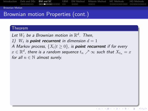
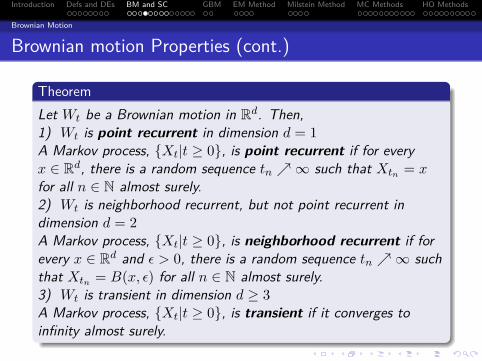
TheoremLet Wt be a Brownian motion in Rd.
Then,1) Wt is point recurrent in dimension d = 1A Markov process, Xt|t ≥ 0, is point recurrent if for everyx ∈ Rd, there is a random sequence tn ∞ such that Xtn = xfor all n ∈ N almost surely.2) Wt is neighborhood recurrent, but not point recurrent indimension d = 2A Markov process, Xt|t ≥ 0, is neighborhood recurrent if forevery x ∈ Rd and ε > 0, there is a random sequence tn ∞ suchthat Xtn = B(x, ε) for all n ∈ N almost surely.3) Wt is transient in dimension d ≥ 3A Markov process, Xt|t ≥ 0, is transient if it converges toinfinity almost surely.
Introduction Defs and DEs BM and SC GBM EM Method Milstein Method MC Methods HO Methods
Brownian Motion
Brownian motion Properties (cont.)
TheoremLet Wt be a Brownian motion in Rd. Then,1) Wt is point recurrent in dimension d = 1
A Markov process, Xt|t ≥ 0, is point recurrent if for everyx ∈ Rd, there is a random sequence tn ∞ such that Xtn = xfor all n ∈ N almost surely.2) Wt is neighborhood recurrent, but not point recurrent indimension d = 2A Markov process, Xt|t ≥ 0, is neighborhood recurrent if forevery x ∈ Rd and ε > 0, there is a random sequence tn ∞ suchthat Xtn = B(x, ε) for all n ∈ N almost surely.3) Wt is transient in dimension d ≥ 3A Markov process, Xt|t ≥ 0, is transient if it converges toinfinity almost surely.
Introduction Defs and DEs BM and SC GBM EM Method Milstein Method MC Methods HO Methods
Brownian Motion
Brownian motion Properties (cont.)
TheoremLet Wt be a Brownian motion in Rd. Then,1) Wt is point recurrent in dimension d = 1A Markov process, Xt|t ≥ 0, is point recurrent if for everyx ∈ Rd, there is a random sequence tn ∞ such that Xtn = xfor all n ∈ N almost surely.
2) Wt is neighborhood recurrent, but not point recurrent indimension d = 2A Markov process, Xt|t ≥ 0, is neighborhood recurrent if forevery x ∈ Rd and ε > 0, there is a random sequence tn ∞ suchthat Xtn = B(x, ε) for all n ∈ N almost surely.3) Wt is transient in dimension d ≥ 3A Markov process, Xt|t ≥ 0, is transient if it converges toinfinity almost surely.
Introduction Defs and DEs BM and SC GBM EM Method Milstein Method MC Methods HO Methods
Brownian Motion
Brownian motion Properties (cont.)
TheoremLet Wt be a Brownian motion in Rd. Then,1) Wt is point recurrent in dimension d = 1A Markov process, Xt|t ≥ 0, is point recurrent if for everyx ∈ Rd, there is a random sequence tn ∞ such that Xtn = xfor all n ∈ N almost surely.2) Wt is neighborhood recurrent, but not point recurrent indimension d = 2
A Markov process, Xt|t ≥ 0, is neighborhood recurrent if forevery x ∈ Rd and ε > 0, there is a random sequence tn ∞ suchthat Xtn = B(x, ε) for all n ∈ N almost surely.3) Wt is transient in dimension d ≥ 3A Markov process, Xt|t ≥ 0, is transient if it converges toinfinity almost surely.
Introduction Defs and DEs BM and SC GBM EM Method Milstein Method MC Methods HO Methods
Brownian Motion
Brownian motion Properties (cont.)
TheoremLet Wt be a Brownian motion in Rd. Then,1) Wt is point recurrent in dimension d = 1A Markov process, Xt|t ≥ 0, is point recurrent if for everyx ∈ Rd, there is a random sequence tn ∞ such that Xtn = xfor all n ∈ N almost surely.2) Wt is neighborhood recurrent, but not point recurrent indimension d = 2A Markov process, Xt|t ≥ 0, is neighborhood recurrent if forevery x ∈ Rd and ε > 0, there is a random sequence tn ∞ suchthat Xtn = B(x, ε) for all n ∈ N almost surely.
3) Wt is transient in dimension d ≥ 3A Markov process, Xt|t ≥ 0, is transient if it converges toinfinity almost surely.
Introduction Defs and DEs BM and SC GBM EM Method Milstein Method MC Methods HO Methods
Brownian Motion
Brownian motion Properties (cont.)
TheoremLet Wt be a Brownian motion in Rd. Then,1) Wt is point recurrent in dimension d = 1A Markov process, Xt|t ≥ 0, is point recurrent if for everyx ∈ Rd, there is a random sequence tn ∞ such that Xtn = xfor all n ∈ N almost surely.2) Wt is neighborhood recurrent, but not point recurrent indimension d = 2A Markov process, Xt|t ≥ 0, is neighborhood recurrent if forevery x ∈ Rd and ε > 0, there is a random sequence tn ∞ suchthat Xtn = B(x, ε) for all n ∈ N almost surely.3) Wt is transient in dimension d ≥ 3
A Markov process, Xt|t ≥ 0, is transient if it converges toinfinity almost surely.
Introduction Defs and DEs BM and SC GBM EM Method Milstein Method MC Methods HO Methods
Brownian Motion
Brownian motion Properties (cont.)
TheoremLet Wt be a Brownian motion in Rd. Then,1) Wt is point recurrent in dimension d = 1A Markov process, Xt|t ≥ 0, is point recurrent if for everyx ∈ Rd, there is a random sequence tn ∞ such that Xtn = xfor all n ∈ N almost surely.2) Wt is neighborhood recurrent, but not point recurrent indimension d = 2A Markov process, Xt|t ≥ 0, is neighborhood recurrent if forevery x ∈ Rd and ε > 0, there is a random sequence tn ∞ suchthat Xtn = B(x, ε) for all n ∈ N almost surely.3) Wt is transient in dimension d ≥ 3A Markov process, Xt|t ≥ 0, is transient if it converges toinfinity almost surely.
Introduction Defs and DEs BM and SC GBM EM Method Milstein Method MC Methods HO Methods
Brownian Motion
Brownian Motion 1D Sample Path
t
0 0.2 0.4 0.6 0.8 1
Wt
-1.6
-1.4
-1.2
-1
-0.8
-0.6
-0.4
-0.2
0
0.2
0.4
Standard Brownian Motion
Introduction Defs and DEs BM and SC GBM EM Method Milstein Method MC Methods HO Methods
Brownian Motion
Brownian Motion in R2 Sample Path
x
-1.4 -1.2 -1 -0.8 -0.6 -0.4 -0.2 0 0.2
y
-0.4
-0.3
-0.2
-0.1
0
0.1
0.2
0.3
0.4
Two dimensional Brownian Motion
Introduction Defs and DEs BM and SC GBM EM Method Milstein Method MC Methods HO Methods
Brownian Motion
Brownian Motion in R3 Sample Path
-0.4-0.3-0.2-0.1
Three dimensional Brownian Motion
0
y
0.10.20.30.4
-1.4
-1.2
-1
-0.8
-0.6
x
-0.4
-0.2
0
0.2
0.2
0
0.1
0.3
0.4
0.5
0.6
0.7
0.8
0.9
z
Introduction Defs and DEs BM and SC GBM EM Method Milstein Method MC Methods HO Methods
Brownian Motion
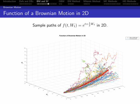
Function of a Brownian Motion in 2D
Sample paths of f(t,Wt) = et+12Wt in 2D.
1
0.9
0.8
0.7
0.6
0.5
t
0.4
Function of Brownian Motion in 2D
0.3
0.2
0.1
00
1
2
3
4
Wt
5
6
7
8
2
0
1
10
9
8
7
6
5
4
3
9
Wt
Mean of 5000 paths
50 individual paths
Introduction Defs and DEs BM and SC GBM EM Method Milstein Method MC Methods HO Methods
Ito and Stratonovich Calculus
Ito CalculusRecall the general SODE
dXt = f(Xt) dt+ F (Xt) dWt for t > 0X0 = x0 x0 ∈ R
Recall that Brownian motion Wt is nowhere differentiable.
DefinitionFor a smooth function, f(t,Xt), the Ito integral of f with respectto standard Brownian motion Wt is given by
∫ t
0fs(s,Xs)dWs = lim
n→∞
n−1∑i=1
f(ti−1, Xti−1)(Wti −Wti−1) (11)
where we evaluate the function f at the left endpoints of somepartition P = 0 = t0 < t1 < . . . < tn = T.
Introduction Defs and DEs BM and SC GBM EM Method Milstein Method MC Methods HO Methods
Ito and Stratonovich Calculus
Ito Lemma (Chain Rule)For a twice differentiable function f(t, x), its Taylor series is
df = ∂f
∂tdt+ ∂f
∂xdx+ 1
2∂2f
∂x2 dx2 + . . . (12)
Assume that dXt = µt dt+ σtdWt. Let x = Xt anddx = µtdt+ σtdWt for dXt, we then get
df(t,Xt) = ∂f
∂tdt+∂f
∂x(µtdt+ σtdWt)
+ 12∂2f
∂x2 (µ2tdt
2 + 2µtσtdtdWt + σ2t dW
2t ) + . . .
Neglecting “small” high order terms such as dtdWt and dW 2t , we
have
df(t,Xt) =(∂f
∂t+ µt
∂f
∂x+ σ2
t
2∂2f
∂x2
)dt+ σt
∂f
∂xdWt
This is Ito’s chain rule.
Introduction Defs and DEs BM and SC GBM EM Method Milstein Method MC Methods HO Methods
Ito and Stratonovich Calculus
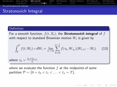
Stratonovich Integral
DefinitionFor a smooth function, f(t,Xt), the Stratonovich integral of fwith respect to standard Brownian motion Wt is given by
∫ T
0f(t,Wt) dWt = lim
n→∞
n−1∑k=0
f(τk,Wτk)(Wt+1 −Wt) (13)
where τk = tk+tk+12 .
where we evaluate the function f at the midpoints of somepartition P = 0 = t0 < t1 < . . . < tn = T.
Introduction Defs and DEs BM and SC GBM EM Method Milstein Method MC Methods HO Methods
Ito and Stratonovich Calculus
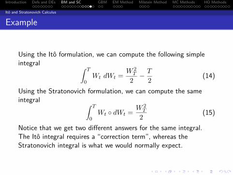
Example
Using the Ito formulation, we can compute the following simpleintegral ∫ T
0Wt dWt = W 2
T
2 − T
2 (14)
Using the Stratonovich formulation, we can compute the sameintegral ∫ T
0Wt dWt = W 2
T
2 (15)
Notice that we get two different answers for the same integral.The Ito integral requires a “correction term”, whereas theStratonovich integral is what we would normally expect.
Introduction Defs and DEs BM and SC GBM EM Method Milstein Method MC Methods HO Methods
Ito and Stratonovich Calculus
Example
Using the Ito formulation, we can compute the following simpleintegral ∫ T
0Wt dWt = W 2
T
2 − T
2 (14)
Using the Stratonovich formulation, we can compute the sameintegral ∫ T
0Wt dWt = W 2
T
2 (15)
Notice that we get two different answers for the same integral.The Ito integral requires a “correction term”, whereas theStratonovich integral is what we would normally expect.
Introduction Defs and DEs BM and SC GBM EM Method Milstein Method MC Methods HO Methods
Ito-Stratonovich Conversion
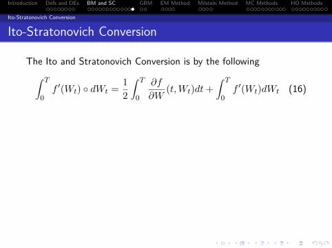
Ito-Stratonovich Conversion
The Ito and Stratonovich Conversion is by the following∫ T
0f ′(Wt) dWt = 1
2
∫ T
0
∂f
∂W(t,Wt)dt+
∫ T
0f ′(Wt)dWt (16)
We can convert from Ito to Stratonovich SODEs or vice versawhenever one is convenient.Definition
dXt
dt= f(t,Xt) + g(t,Xt) ξ (Ito) (17)
dXt
dt= (f(t,Xt)−
12g(t,Xt)
∂
∂Xtg(t,Xt)) + g(t,Xt) ξ (18)
(Stratonovich)
Introduction Defs and DEs BM and SC GBM EM Method Milstein Method MC Methods HO Methods
Ito-Stratonovich Conversion
Ito-Stratonovich Conversion
The Ito and Stratonovich Conversion is by the following∫ T
0f ′(Wt) dWt = 1
2
∫ T
0
∂f
∂W(t,Wt)dt+
∫ T
0f ′(Wt)dWt (16)
We can convert from Ito to Stratonovich SODEs or vice versawhenever one is convenient.Definition
dXt
dt= f(t,Xt) + g(t,Xt) ξ (Ito) (17)
dXt
dt= (f(t,Xt)−
12g(t,Xt)
∂
∂Xtg(t,Xt)) + g(t,Xt) ξ (18)
(Stratonovich)
Introduction Defs and DEs BM and SC GBM EM Method Milstein Method MC Methods HO Methods
Geometric Brownian Motion
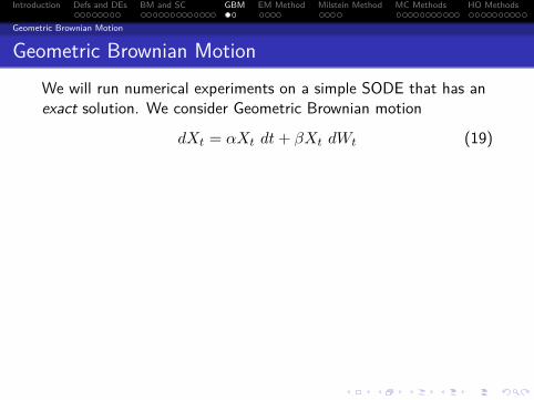
Geometric Brownian MotionWe will run numerical experiments on a simple SODE that has anexact solution. We consider Geometric Brownian motion
dXt = αXt dt+ βXt dWt (19)
ExampleWe seek an exact solution to the above SODE. By computation,we have
dXt
Xt= α dt+ β dWt∫ t
0
dXs
Xs= α t+ β Wt∫ t
0d(log(Xs))ds = α t+ β Wt
Introduction Defs and DEs BM and SC GBM EM Method Milstein Method MC Methods HO Methods
Geometric Brownian Motion
Geometric Brownian Motion (cont.)
Example
∫ t
0d(log(Xs))ds = α t+ β Wt
log(Xt)−12β
2t = α t+ β Wt
Xt = x0eβWt+
(α−β
22
)t
where we have used a direct application of Ito’s chain rule:
d(log(Xs)) = dXs
Xs− 1
2β2X2
sdt
X2s
. (20)
Introduction Defs and DEs BM and SC GBM EM Method Milstein Method MC Methods HO Methods
Euler-Maruyama Method
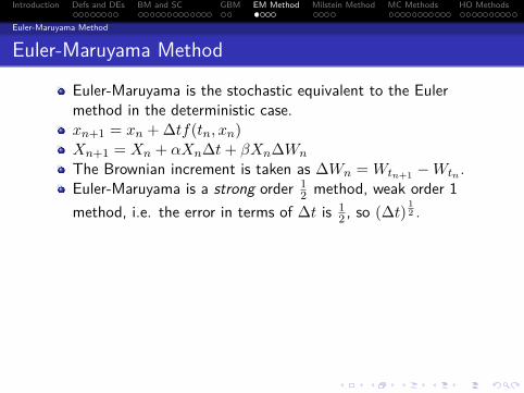
Euler-Maruyama Method
Euler-Maruyama is the stochastic equivalent to the Eulermethod in the deterministic case.xn+1 = xn + ∆tf(tn, xn)
Xn+1 = Xn + αXn∆t+ βXn∆Wn
The Brownian increment is taken as ∆Wn = Wtn+1 −Wtn .Euler-Maruyama is a strong order 1
2 method, weak order 1method, i.e. the error in terms of ∆t is 1
2 , so (∆t)12 .
A method has a strong order of convergence equal to γ ifthere exists a constant C such that
E|Xn −XT | ≤ C∆tγ (21)A method has a weak order of convergence equal to γ if thereexists a constant C such that
|Ep(Xn)− Ep(XT )| ≤ C∆tγ (22)
Introduction Defs and DEs BM and SC GBM EM Method Milstein Method MC Methods HO Methods
Euler-Maruyama Method
Euler-Maruyama Method
Euler-Maruyama is the stochastic equivalent to the Eulermethod in the deterministic case.xn+1 = xn + ∆tf(tn, xn)Xn+1 = Xn + αXn∆t+ βXn∆Wn
The Brownian increment is taken as ∆Wn = Wtn+1 −Wtn .
Euler-Maruyama is a strong order 12 method, weak order 1
method, i.e. the error in terms of ∆t is 12 , so (∆t)
12 .
A method has a strong order of convergence equal to γ ifthere exists a constant C such that
E|Xn −XT | ≤ C∆tγ (21)A method has a weak order of convergence equal to γ if thereexists a constant C such that
|Ep(Xn)− Ep(XT )| ≤ C∆tγ (22)
Introduction Defs and DEs BM and SC GBM EM Method Milstein Method MC Methods HO Methods
Euler-Maruyama Method
Euler-Maruyama Method
Euler-Maruyama is the stochastic equivalent to the Eulermethod in the deterministic case.xn+1 = xn + ∆tf(tn, xn)Xn+1 = Xn + αXn∆t+ βXn∆Wn
The Brownian increment is taken as ∆Wn = Wtn+1 −Wtn .Euler-Maruyama is a strong order 1
2 method, weak order 1method, i.e. the error in terms of ∆t is 1
2 , so (∆t)12 .
A method has a strong order of convergence equal to γ ifthere exists a constant C such that
E|Xn −XT | ≤ C∆tγ (21)A method has a weak order of convergence equal to γ if thereexists a constant C such that
|Ep(Xn)− Ep(XT )| ≤ C∆tγ (22)
Introduction Defs and DEs BM and SC GBM EM Method Milstein Method MC Methods HO Methods
Euler-Maruyama Method
Euler-Maruyama Method
Euler-Maruyama is the stochastic equivalent to the Eulermethod in the deterministic case.xn+1 = xn + ∆tf(tn, xn)Xn+1 = Xn + αXn∆t+ βXn∆Wn
The Brownian increment is taken as ∆Wn = Wtn+1 −Wtn .Euler-Maruyama is a strong order 1
2 method, weak order 1method, i.e. the error in terms of ∆t is 1
2 , so (∆t)12 .
A method has a strong order of convergence equal to γ ifthere exists a constant C such that
E|Xn −XT | ≤ C∆tγ (21)
A method has a weak order of convergence equal to γ if thereexists a constant C such that
|Ep(Xn)− Ep(XT )| ≤ C∆tγ (22)
Introduction Defs and DEs BM and SC GBM EM Method Milstein Method MC Methods HO Methods
Euler-Maruyama Method
Euler-Maruyama Method
Euler-Maruyama is the stochastic equivalent to the Eulermethod in the deterministic case.xn+1 = xn + ∆tf(tn, xn)Xn+1 = Xn + αXn∆t+ βXn∆Wn
The Brownian increment is taken as ∆Wn = Wtn+1 −Wtn .Euler-Maruyama is a strong order 1
2 method, weak order 1method, i.e. the error in terms of ∆t is 1
2 , so (∆t)12 .
A method has a strong order of convergence equal to γ ifthere exists a constant C such that
E|Xn −XT | ≤ C∆tγ (21)A method has a weak order of convergence equal to γ if thereexists a constant C such that
|Ep(Xn)− Ep(XT )| ≤ C∆tγ (22)
Introduction Defs and DEs BM and SC GBM EM Method Milstein Method MC Methods HO Methods
Euler-Maruyama Method
Euler-Maruyama Results
t
0 0.1 0.2 0.3 0.4 0.5 0.6 0.7 0.8 0.9 1
Xt
0.5
1
1.5
2
2.5
3
3.5
4
Euler-Maruyama Approximation
Figure : Estimation with time step 10−2
Introduction Defs and DEs BM and SC GBM EM Method Milstein Method MC Methods HO Methods
Euler-Maruyama Method
Euler-Maruyama Results (cont.)
log( ∆ t)10 -3 10 -2 10 -1
log(e
rror)
10 -2
10 -1
10 0Strong Error for EM
Figure : Log-log plot of error for various time steps. Red reference line isslope 1/2.
Introduction Defs and DEs BM and SC GBM EM Method Milstein Method MC Methods HO Methods
Euler-Maruyama Method
Euler-Maruyama Results (cont.)
log( ∆ t)10 -4 10 -3 10 -2 10 -1
log(e
rror)
10 -4
10 -3
10 -2
10 -1
10 0Weak Error for EM
Figure : Log-log plot of error for various time steps. Red reference line isslope 1.
Introduction Defs and DEs BM and SC GBM EM Method Milstein Method MC Methods HO Methods
Milstein Method
Milstein Method
Milstein is identical to the Euler-Maruyama method if there isno Xt term in front of the Brownian motion.
Milstein is a Taylor method and is a truncation of thestochastic Taylor expansion of the solution that we have seenpreviously.Xn+1 = Xn + αXn∆t+ βXn∆Wn + 1
2β2Xn((∆Wn)2 −∆t)
Again, the Brownian increment is taken as∆Wn = Wtn+1 −Wtn .The Milstein method is a strong and weak 1.0 method.
Introduction Defs and DEs BM and SC GBM EM Method Milstein Method MC Methods HO Methods
Milstein Method
Milstein Method
Milstein is identical to the Euler-Maruyama method if there isno Xt term in front of the Brownian motion.Milstein is a Taylor method and is a truncation of thestochastic Taylor expansion of the solution that we have seenpreviously.
Xn+1 = Xn + αXn∆t+ βXn∆Wn + 12β
2Xn((∆Wn)2 −∆t)Again, the Brownian increment is taken as∆Wn = Wtn+1 −Wtn .The Milstein method is a strong and weak 1.0 method.
Introduction Defs and DEs BM and SC GBM EM Method Milstein Method MC Methods HO Methods
Milstein Method
Milstein Method
Milstein is identical to the Euler-Maruyama method if there isno Xt term in front of the Brownian motion.Milstein is a Taylor method and is a truncation of thestochastic Taylor expansion of the solution that we have seenpreviously.Xn+1 = Xn + αXn∆t+ βXn∆Wn + 1
2β2Xn((∆Wn)2 −∆t)
Again, the Brownian increment is taken as∆Wn = Wtn+1 −Wtn .The Milstein method is a strong and weak 1.0 method.
Introduction Defs and DEs BM and SC GBM EM Method Milstein Method MC Methods HO Methods
Milstein Method
Milstein Method
Milstein is identical to the Euler-Maruyama method if there isno Xt term in front of the Brownian motion.Milstein is a Taylor method and is a truncation of thestochastic Taylor expansion of the solution that we have seenpreviously.Xn+1 = Xn + αXn∆t+ βXn∆Wn + 1
2β2Xn((∆Wn)2 −∆t)
Again, the Brownian increment is taken as∆Wn = Wtn+1 −Wtn .
The Milstein method is a strong and weak 1.0 method.
Introduction Defs and DEs BM and SC GBM EM Method Milstein Method MC Methods HO Methods
Milstein Method
Milstein Method
Milstein is identical to the Euler-Maruyama method if there isno Xt term in front of the Brownian motion.Milstein is a Taylor method and is a truncation of thestochastic Taylor expansion of the solution that we have seenpreviously.Xn+1 = Xn + αXn∆t+ βXn∆Wn + 1
2β2Xn((∆Wn)2 −∆t)
Again, the Brownian increment is taken as∆Wn = Wtn+1 −Wtn .The Milstein method is a strong and weak 1.0 method.
Introduction Defs and DEs BM and SC GBM EM Method Milstein Method MC Methods HO Methods
Milstein Method
Milstein Method Results
t
0 0.1 0.2 0.3 0.4 0.5 0.6 0.7 0.8 0.9 1
Xt
0.5
1
1.5
2
2.5
3
3.5
Milstein Approximation
Figure : Estimation with time step 10−2
Introduction Defs and DEs BM and SC GBM EM Method Milstein Method MC Methods HO Methods
Milstein Method
Milstein Method Results (cont.)
log( ∆ t)10 -3 10 -2 10 -1
log(e
rror)
10 -3
10 -2
10 -1
10 0Strong Error for Milstein
Figure : Log-log plot of error for various time steps. Red reference line isslope 1.
Introduction Defs and DEs BM and SC GBM EM Method Milstein Method MC Methods HO Methods
Milstein Method
Milstein Method Results (cont.)
log( ∆ t)10 -4 10 -3 10 -2 10 -1
log(e
rror)
10 -4
10 -3
10 -2
10 -1
10 0Weak Error for Milstein
Figure : Log-log plot of error for various time steps. Red reference line isslope 1.
Introduction Defs and DEs BM and SC GBM EM Method Milstein Method MC Methods HO Methods
Monte Carlo Methods
Monte Carlo Methods
Monte Carlo methods repeat a process with different inputdata and then average separate outputs, Xj to find anapproximation to the true mean, XM = (X1 + . . .+XM )/M .Commonly, the program uses inputs that are produced by arandom number generator.
For a well designed process, the approximation of the meanwill converge to the true mean as the number of samples, M ,increases.Two implementations of Monte Carlo methods will be given
1 Numerical Approximation of the Logistic Equation withrandom initial data
2 Approximation of Geometric Brownian Motion
Introduction Defs and DEs BM and SC GBM EM Method Milstein Method MC Methods HO Methods
Monte Carlo Methods
Monte Carlo Methods
Monte Carlo methods repeat a process with different inputdata and then average separate outputs, Xj to find anapproximation to the true mean, XM = (X1 + . . .+XM )/M .Commonly, the program uses inputs that are produced by arandom number generator.For a well designed process, the approximation of the meanwill converge to the true mean as the number of samples, M ,increases.
Two implementations of Monte Carlo methods will be given
1 Numerical Approximation of the Logistic Equation withrandom initial data
2 Approximation of Geometric Brownian Motion
Introduction Defs and DEs BM and SC GBM EM Method Milstein Method MC Methods HO Methods
Monte Carlo Methods
Monte Carlo Methods
Monte Carlo methods repeat a process with different inputdata and then average separate outputs, Xj to find anapproximation to the true mean, XM = (X1 + . . .+XM )/M .Commonly, the program uses inputs that are produced by arandom number generator.For a well designed process, the approximation of the meanwill converge to the true mean as the number of samples, M ,increases.Two implementations of Monte Carlo methods will be given
1 Numerical Approximation of the Logistic Equation withrandom initial data
2 Approximation of Geometric Brownian Motion
Introduction Defs and DEs BM and SC GBM EM Method Milstein Method MC Methods HO Methods
Monte Carlo Methods
Convergence Rate
The Monte Carlo Method has convergence rate of O(M−1/2).This convergence rate is emphasized via the root-mean squared(RMS), via the formula
√E((µM − µ)2) = σM√
M(23)
where the numerical variance, σ2M can be calculated using the
following formula
σ2M = 1
M − 1
M∑j=1
(Xj − XM
)2(24)
Introduction Defs and DEs BM and SC GBM EM Method Milstein Method MC Methods HO Methods
Monte Carlo Methods
Convergence Rate
The Monte Carlo Method has convergence rate of O(M−1/2).This convergence rate is emphasized via the root-mean squared(RMS), via the formula√
E((µM − µ)2) = σM√M
(23)
where the numerical variance, σ2M can be calculated using the
following formula
σ2M = 1
M − 1
M∑j=1
(Xj − XM
)2(24)
Introduction Defs and DEs BM and SC GBM EM Method Milstein Method MC Methods HO Methods
Monte Carlo Methods
Approximation of the Logistic Equation
Using the Monte Carlo method we want to numericallyapproximate the solution to the Logistic Equation with randominitial data:
dydt = y(t)(1− y(t)) in [0, T ]y(0) = y0 ∼ U(D) D = [1
2 − ε,12 + ε]
where we take T = 10 and ε = 0.1. The term U(D) denotes thatwe will choose y0 independently from a uniform distribution on theset D, as defined above.
Introduction Defs and DEs BM and SC GBM EM Method Milstein Method MC Methods HO Methods
Monte Carlo Methods
Approximation of the Logistic Equation (cont.)
The value of ε is chosen to such that some “error” is incurredwhen measuring the initial data, say for some population.
ExampleThe mean of the random initial data can be calculated as follows:
y0 = 12(b− a) = 1
2
(12 − ε+ 1
2 + ε
)= 1
2
The true solution of the IVP is known for the mean, y0
y(t) = et
et + 1
So we takeE [y(T )] = eT
eT + 1
Introduction Defs and DEs BM and SC GBM EM Method Milstein Method MC Methods HO Methods
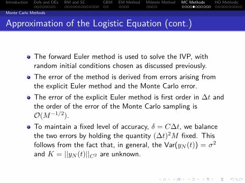
Monte Carlo Methods
Approximation of the Logistic Equation (cont.)
The forward Euler method is used to solve the IVP, withrandom initial conditions chosen as discussed previously.
The error of the method is derived from errors arising fromthe explicit Euler method and the Monte Carlo error.The error of the explicit Euler method is first order in ∆t andthe order of the error of the Monte Carlo sampling isO(M−1/2).To maintain a fixed level of accuracy, δ = C∆t, we balancethe two errors by holding the quantity (∆t)2M fixed. Thisfollows from the fact that, in general, the Var(yN (t)) = σ2
and K = ||yN (t)||C2 are unknown.
Introduction Defs and DEs BM and SC GBM EM Method Milstein Method MC Methods HO Methods
Monte Carlo Methods
Approximation of the Logistic Equation (cont.)
The forward Euler method is used to solve the IVP, withrandom initial conditions chosen as discussed previously.The error of the method is derived from errors arising fromthe explicit Euler method and the Monte Carlo error.
The error of the explicit Euler method is first order in ∆t andthe order of the error of the Monte Carlo sampling isO(M−1/2).To maintain a fixed level of accuracy, δ = C∆t, we balancethe two errors by holding the quantity (∆t)2M fixed. Thisfollows from the fact that, in general, the Var(yN (t)) = σ2
and K = ||yN (t)||C2 are unknown.
Introduction Defs and DEs BM and SC GBM EM Method Milstein Method MC Methods HO Methods
Monte Carlo Methods
Approximation of the Logistic Equation (cont.)
The forward Euler method is used to solve the IVP, withrandom initial conditions chosen as discussed previously.The error of the method is derived from errors arising fromthe explicit Euler method and the Monte Carlo error.The error of the explicit Euler method is first order in ∆t andthe order of the error of the Monte Carlo sampling isO(M−1/2).
To maintain a fixed level of accuracy, δ = C∆t, we balancethe two errors by holding the quantity (∆t)2M fixed. Thisfollows from the fact that, in general, the Var(yN (t)) = σ2
and K = ||yN (t)||C2 are unknown.
Introduction Defs and DEs BM and SC GBM EM Method Milstein Method MC Methods HO Methods
Monte Carlo Methods
Approximation of the Logistic Equation (cont.)
The forward Euler method is used to solve the IVP, withrandom initial conditions chosen as discussed previously.The error of the method is derived from errors arising fromthe explicit Euler method and the Monte Carlo error.The error of the explicit Euler method is first order in ∆t andthe order of the error of the Monte Carlo sampling isO(M−1/2).To maintain a fixed level of accuracy, δ = C∆t, we balancethe two errors by holding the quantity (∆t)2M fixed. Thisfollows from the fact that, in general, the Var(yN (t)) = σ2
and K = ||yN (t)||C2 are unknown.
Introduction Defs and DEs BM and SC GBM EM Method Milstein Method MC Methods HO Methods
Monte Carlo Methods
Approximation of the Logistic Equation (cont.)
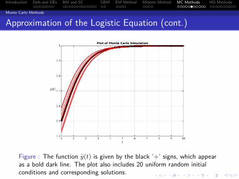
Figure : The function y(t) is given by the black ‘+’ signs, which appearas a bold dark line. The plot also includes 20 uniform random initialconditions and corresponding solutions.
Introduction Defs and DEs BM and SC GBM EM Method Milstein Method MC Methods HO Methods
Monte Carlo Methods
Approximation of the Logistic Equation (cont.)
Figure : Forward Euler is used with (∆t)2M = constant. The blue line isthe reference for slope of -1. The red is the approximation of the errorwhich is first order in ∆t.
Introduction Defs and DEs BM and SC GBM EM Method Milstein Method MC Methods HO Methods
Monte Carlo Methods
Approximation of Geometric Brownian Motion
Using the Monte Carlo method we want to numericallyapproximate the solution to the Geometric Brownian motion SODE
dXt = αXtdt+ βXtdWt
X0 = .5
where the exact solution to the SODE is given by
Xt = X0e(α−β
22 )t+αWt (25)
For simplicity, we take T = 1. The parameters will be taken asα = 2, β = 0.1.
Introduction Defs and DEs BM and SC GBM EM Method Milstein Method MC Methods HO Methods
Monte Carlo Methods
Approximation of Geometric Brownian Motion (cont.)
The Monte Carlo method is used when we want to have aweak approximation of the solution to the SODE. In this casewe will follow what was done with the deterministic logisticequation with random initial data.
If we want the weak approximation of the solution to theSODE, we must use multiple paths, since the quantity ofinterest will be E[XT ].
DefinitionA method has weak order convergence of γ if there exists aconstant C such that for all functions p in some class
|E[p(Xn)]− E[p(Xτ )]| ≤ C∆tγ (26)
at any fixed τ = n∆t ∈ [0, T ] and ∆t sufficiently small.
Introduction Defs and DEs BM and SC GBM EM Method Milstein Method MC Methods HO Methods
Monte Carlo Methods
Approximation of Geometric Brownian Motion (cont.)
The Monte Carlo method is used when we want to have aweak approximation of the solution to the SODE. In this casewe will follow what was done with the deterministic logisticequation with random initial data.If we want the weak approximation of the solution to theSODE, we must use multiple paths, since the quantity ofinterest will be E[XT ].
DefinitionA method has weak order convergence of γ if there exists aconstant C such that for all functions p in some class
|E[p(Xn)]− E[p(Xτ )]| ≤ C∆tγ (26)
at any fixed τ = n∆t ∈ [0, T ] and ∆t sufficiently small.
Introduction Defs and DEs BM and SC GBM EM Method Milstein Method MC Methods HO Methods
Monte Carlo Methods
Approximation of Geometric Brownian Motion (cont.)
Figure : Sample paths for M = 500 for the solution to the GeometricBrownian motion. The value of E[XT ] = eµT = e2. The dark linerepresents the function y(t) = e2t.
Introduction Defs and DEs BM and SC GBM EM Method Milstein Method MC Methods HO Methods
Monte Carlo Methods
Approximation of Geometric Brownian Motion (cont.)
Figure : Weak Approximation error for GBM. The red reference line isthat of slope 1.
Introduction Defs and DEs BM and SC GBM EM Method Milstein Method MC Methods HO Methods
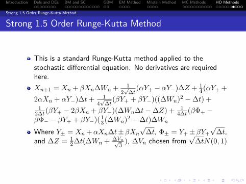
Strong 1.0 Order Runge-Kutta Method
Strong 1.0 Order Runge-Kutta Method
This is a standard Runge-Kutta method applied to thestochastic differential equation.
Xn+1 = Xn + αXn∆t+ βXn∆Wn
+ 12β
2(β(Xn + βXn
√∆t)− βXn)((∆Wn)2 −∆t)√
∆t
Of course by the name, the method is of strong order 1.0.
Introduction Defs and DEs BM and SC GBM EM Method Milstein Method MC Methods HO Methods
Strong 1.0 Order Runge-Kutta Method
Strong 1.0 Order Runge-Kutta Method
This is a standard Runge-Kutta method applied to thestochastic differential equation.
Xn+1 = Xn + αXn∆t+ βXn∆Wn
+ 12β
2(β(Xn + βXn
√∆t)− βXn)((∆Wn)2 −∆t)√
∆t
Of course by the name, the method is of strong order 1.0.
Introduction Defs and DEs BM and SC GBM EM Method Milstein Method MC Methods HO Methods
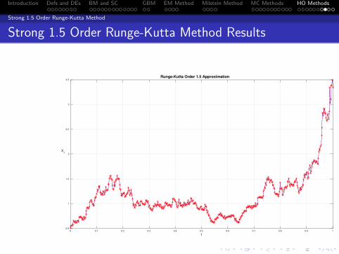
Strong 1.0 Order Runge-Kutta Method
Strong 1.0 Order Runge-Kutta Method Results
t
0 0.1 0.2 0.3 0.4 0.5 0.6 0.7 0.8 0.9 1
Xt
0.5
1
1.5
2
2.5
3
3.5
Runge-Kutta Order 1.0 Approximation
Figure : Estimation with time step 10−2
Introduction Defs and DEs BM and SC GBM EM Method Milstein Method MC Methods HO Methods
Strong 1.0 Order Runge-Kutta Method
Strong 1.0 Order Runge-Kutta Method Results
log( ∆ t)10 -3 10 -2 10 -1
log(e
rror)
10 -3
10 -2
10 -1
10 0Strong Error for Runge-Kutta Order 1.0
Figure : Log-log plot of error for various time steps. The red referenceline is that of slope 1.
Introduction Defs and DEs BM and SC GBM EM Method Milstein Method MC Methods HO Methods
Taylor Method Order 1.5
Strong 1.5 Order Taylor Method
This is a Taylor method of higher order, meaning morederivatives are needed.
When initial conditions are known with accuracy, higher ordermethods yield better numerical approximations even thoughthey are complex.If initial conditions are chosen from a probability distribution,the advantages of the higher order method are not asbeneficial, and computationally expensive.Xn+1 = Xn + αXn∆t+ βXn∆Wn + 1
2β2Xn((∆Wn)2 −
∆t) + αβXn∆Z + 12α
2Xn(∆t)2 + αβXn(∆Wn∆t−∆Z) +12β
3Xn(13(∆Wn)2 −∆t)∆Wn
Where ∆Z = 12∆t(∆Wn + ∆Vn√
3 ), ∆Vn chosen from√
∆tN(0, 1)Again, by the name, this is a strong order 1.5 method.
Introduction Defs and DEs BM and SC GBM EM Method Milstein Method MC Methods HO Methods
Taylor Method Order 1.5
Strong 1.5 Order Taylor Method
This is a Taylor method of higher order, meaning morederivatives are needed.When initial conditions are known with accuracy, higher ordermethods yield better numerical approximations even thoughthey are complex.
If initial conditions are chosen from a probability distribution,the advantages of the higher order method are not asbeneficial, and computationally expensive.Xn+1 = Xn + αXn∆t+ βXn∆Wn + 1
2β2Xn((∆Wn)2 −
∆t) + αβXn∆Z + 12α
2Xn(∆t)2 + αβXn(∆Wn∆t−∆Z) +12β
3Xn(13(∆Wn)2 −∆t)∆Wn
Where ∆Z = 12∆t(∆Wn + ∆Vn√
3 ), ∆Vn chosen from√
∆tN(0, 1)Again, by the name, this is a strong order 1.5 method.
Introduction Defs and DEs BM and SC GBM EM Method Milstein Method MC Methods HO Methods
Taylor Method Order 1.5
Strong 1.5 Order Taylor Method
This is a Taylor method of higher order, meaning morederivatives are needed.When initial conditions are known with accuracy, higher ordermethods yield better numerical approximations even thoughthey are complex.If initial conditions are chosen from a probability distribution,the advantages of the higher order method are not asbeneficial, and computationally expensive.
Xn+1 = Xn + αXn∆t+ βXn∆Wn + 12β
2Xn((∆Wn)2 −∆t) + αβXn∆Z + 1
2α2Xn(∆t)2 + αβXn(∆Wn∆t−∆Z) +
12β
3Xn(13(∆Wn)2 −∆t)∆Wn
Where ∆Z = 12∆t(∆Wn + ∆Vn√
3 ), ∆Vn chosen from√
∆tN(0, 1)Again, by the name, this is a strong order 1.5 method.
Introduction Defs and DEs BM and SC GBM EM Method Milstein Method MC Methods HO Methods
Taylor Method Order 1.5
Strong 1.5 Order Taylor Method
This is a Taylor method of higher order, meaning morederivatives are needed.When initial conditions are known with accuracy, higher ordermethods yield better numerical approximations even thoughthey are complex.If initial conditions are chosen from a probability distribution,the advantages of the higher order method are not asbeneficial, and computationally expensive.Xn+1 = Xn + αXn∆t+ βXn∆Wn + 1
2β2Xn((∆Wn)2 −
∆t) + αβXn∆Z + 12α
2Xn(∆t)2 + αβXn(∆Wn∆t−∆Z) +12β
3Xn(13(∆Wn)2 −∆t)∆Wn
Where ∆Z = 12∆t(∆Wn + ∆Vn√
3 ), ∆Vn chosen from√
∆tN(0, 1)Again, by the name, this is a strong order 1.5 method.
Introduction Defs and DEs BM and SC GBM EM Method Milstein Method MC Methods HO Methods
Taylor Method Order 1.5
Strong 1.5 Order Taylor Method
This is a Taylor method of higher order, meaning morederivatives are needed.When initial conditions are known with accuracy, higher ordermethods yield better numerical approximations even thoughthey are complex.If initial conditions are chosen from a probability distribution,the advantages of the higher order method are not asbeneficial, and computationally expensive.Xn+1 = Xn + αXn∆t+ βXn∆Wn + 1
2β2Xn((∆Wn)2 −
∆t) + αβXn∆Z + 12α
2Xn(∆t)2 + αβXn(∆Wn∆t−∆Z) +12β
3Xn(13(∆Wn)2 −∆t)∆Wn
Where ∆Z = 12∆t(∆Wn + ∆Vn√
3 ), ∆Vn chosen from√
∆tN(0, 1)
Again, by the name, this is a strong order 1.5 method.
Introduction Defs and DEs BM and SC GBM EM Method Milstein Method MC Methods HO Methods
Taylor Method Order 1.5
Strong 1.5 Order Taylor Method
This is a Taylor method of higher order, meaning morederivatives are needed.When initial conditions are known with accuracy, higher ordermethods yield better numerical approximations even thoughthey are complex.If initial conditions are chosen from a probability distribution,the advantages of the higher order method are not asbeneficial, and computationally expensive.Xn+1 = Xn + αXn∆t+ βXn∆Wn + 1
2β2Xn((∆Wn)2 −
∆t) + αβXn∆Z + 12α
2Xn(∆t)2 + αβXn(∆Wn∆t−∆Z) +12β
3Xn(13(∆Wn)2 −∆t)∆Wn
Where ∆Z = 12∆t(∆Wn + ∆Vn√
3 ), ∆Vn chosen from√
∆tN(0, 1)Again, by the name, this is a strong order 1.5 method.
Introduction Defs and DEs BM and SC GBM EM Method Milstein Method MC Methods HO Methods
Taylor Method Order 1.5
Strong 1.5 Order Taylor Method Results
t
0 0.1 0.2 0.3 0.4 0.5 0.6 0.7 0.8 0.9 1
Xt
0.5
1
1.5
2
2.5
3
3.5
Taylor Order 1.5 Approximation
Figure : Estimation with time step 10−2
Introduction Defs and DEs BM and SC GBM EM Method Milstein Method MC Methods HO Methods
Taylor Method Order 1.5
Strong 1.5 Order Taylor Method Results
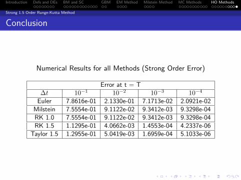
log( ∆ t)10 -3 10 -2 10 -1
log(e
rror)
10 -5
10 -4
10 -3
10 -2
10 -1Strong Error for Taylor Order 1.5
Figure : Log-log plot of error for various time steps. The red referenceline is that of slope 1.5.
Introduction Defs and DEs BM and SC GBM EM Method Milstein Method MC Methods HO Methods
Strong 1.5 Order Runge-Kutta Method
Strong 1.5 Order Runge-Kutta Method
This is a standard Runge-Kutta method applied to thestochastic differential equation. No derivatives are requiredhere.
Xn+1 = Xn + βXn∆Wn + 12√
∆t(αY+ − αY−)∆Z + 14(αY+ +
2αXn + αY−)∆t+ 14√
∆t(βY+ + βY−)((∆Wn)2 −∆t) +1
2∆t(βY+ − 2βXn + βY−)(∆Wn∆t−∆Z) + 14∆t(βΦ+ −
βΦ− − βY+ + βY−)(13(∆Wn)2 −∆t)∆Wn
Where Y± = Xn +αXn∆t±βXn
√∆t, Φ± = Y+±βY+
√∆t,
and ∆Z = 12∆t(∆Wn + ∆Vn√
3 ), ∆Vn chosen from√
∆tN(0, 1)This is a strong order 1.5 method.
Introduction Defs and DEs BM and SC GBM EM Method Milstein Method MC Methods HO Methods
Strong 1.5 Order Runge-Kutta Method
Strong 1.5 Order Runge-Kutta Method
This is a standard Runge-Kutta method applied to thestochastic differential equation. No derivatives are requiredhere.Xn+1 = Xn + βXn∆Wn + 1
2√
∆t(αY+ − αY−)∆Z + 14(αY+ +
2αXn + αY−)∆t+ 14√
∆t(βY+ + βY−)((∆Wn)2 −∆t) +1
2∆t(βY+ − 2βXn + βY−)(∆Wn∆t−∆Z) + 14∆t(βΦ+ −
βΦ− − βY+ + βY−)(13(∆Wn)2 −∆t)∆Wn
Where Y± = Xn +αXn∆t±βXn
√∆t, Φ± = Y+±βY+
√∆t,
and ∆Z = 12∆t(∆Wn + ∆Vn√
3 ), ∆Vn chosen from√
∆tN(0, 1)
This is a strong order 1.5 method.
Introduction Defs and DEs BM and SC GBM EM Method Milstein Method MC Methods HO Methods
Strong 1.5 Order Runge-Kutta Method
Strong 1.5 Order Runge-Kutta Method
This is a standard Runge-Kutta method applied to thestochastic differential equation. No derivatives are requiredhere.Xn+1 = Xn + βXn∆Wn + 1
2√
∆t(αY+ − αY−)∆Z + 14(αY+ +
2αXn + αY−)∆t+ 14√
∆t(βY+ + βY−)((∆Wn)2 −∆t) +1
2∆t(βY+ − 2βXn + βY−)(∆Wn∆t−∆Z) + 14∆t(βΦ+ −
βΦ− − βY+ + βY−)(13(∆Wn)2 −∆t)∆Wn
Where Y± = Xn +αXn∆t±βXn
√∆t, Φ± = Y+±βY+
√∆t,
and ∆Z = 12∆t(∆Wn + ∆Vn√
3 ), ∆Vn chosen from√
∆tN(0, 1)This is a strong order 1.5 method.
Introduction Defs and DEs BM and SC GBM EM Method Milstein Method MC Methods HO Methods
Strong 1.5 Order Runge-Kutta Method
Strong 1.5 Order Runge-Kutta Method Results
t
0 0.1 0.2 0.3 0.4 0.5 0.6 0.7 0.8 0.9 1
Xt
0.5
1
1.5
2
2.5
3
3.5
Runge-Kutta Order 1.5 Approximation
Figure : Estimation with time step 10−2
Introduction Defs and DEs BM and SC GBM EM Method Milstein Method MC Methods HO Methods
Strong 1.5 Order Runge-Kutta Method
Strong 1.5 Order Runge-Kutta Method Results
log( ∆ t)10 -3 10 -2 10 -1
log(e
rror)
10 -5
10 -4
10 -3
10 -2
10 -1Strong Error for Runge-Kutta Order 1.5
Figure : Log-log plot of error for various time steps. The red referenceline is that of slope 1.5.
Introduction Defs and DEs BM and SC GBM EM Method Milstein Method MC Methods HO Methods
Strong 1.5 Order Runge-Kutta Method
Conclusion
Numerical Results for all Methods (Strong Order Error)