Numerical MHD of Aircraft Re-entry; Fluid Dynamic, Electromagnetic and

Chemical EffectsG. Seller

Dipartimento di Scienze e Tecnologie Fisiche ed Energetiche, Tor Vergata University, Italy

M. Capitelli, S. LongoChemistry Department, Bari University, Italy

I. ArmeniseIMIP-CNR, Bari, Italy

Magnetohydrodynamics• Fluid dynamics

• Electromagnetism

• Chemistry

• Physical behavior of Plasma (Generalized Ohm Law or other)

Fluid dynamics for MHD and other applicationsFinite difference method. Space-centred explicit scheme of first order with numerical

stiffness

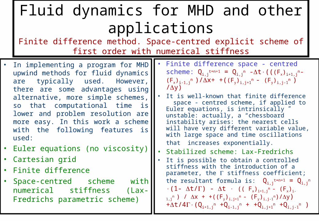
• In implementing a program for MHD upwind methods for fluid dynamics are typically used. However, there are some advantages using alternative, more simple schemes, so that computational time is lower and problem resolution are more easy. In this work a scheme with the following features is used:

• Euler equations (no viscosity)

• Cartesian grid

• Finite difference

• Space-centred scheme with numerical stiffness (Lax-Fredrichs parametric scheme)

• Finite difference space - centred scheme: Qi,j

t=n+1 = Qi,jn -t(((Fx)i+1,j

n- (Fx)i-1,jn

)/x+ +((Fy)i,j+1

n - (Fy)i,j-1

n ) /y)

• It is well-known that finite difference space - centred scheme, if applied to Euler equations, is intrinsically unstable: actually, a “chessboard” instability arises: the nearest cells will have very different variable value, with large space and time oscillations that increases exponentially.

• Stabilized scheme: Lax-Fredrichs• It is possible to obtain a controlled stiffness with

the introduction of a parameter, the stiffness coefficient; the resultant formula is: Qi,j

t=n+1 = Qi,j

n (1- t/) - t (( Fx)i+1,jn - (Fx)i-1,j

n ) / x +

+((Fy)i,j+1n

- (Fy)i,j-1n)/y) +t/4(Qi+1,j

n +Qi-1,jn

+ +Qi,j+1n +Qi,j-1

n )

Advantages with modified Lax-Fredrichs scheme

• First order scheme, without oscillations near discontinuity– (This is important MHD: actually Brio e Wu (1981) found a complex structure in MHD

shock waves (compound waves with compressions and expansions). This structure is not identifiable in a second order scheme (Lax - Wendroff) because of the numerical oscillation)

• The scheme simplicity is computational time-saving.• The scheme is extremely flexible, so that implementation of new condition and equation (as

Maxwell equation for MHD and chemistry) is very easy. • Actually, a simple ad-hoc, computational time-saving Maxwell solver has been implemented.

The scheme has been validate by comparison with results of an upwind scheme and with results of a particle method.

Comparison between results of a MHD and a particle scheme in a simple fluid dynamic, time-dependent case.

Two-dimensional expansion of a circular blast of high density in a reflective square box.

Initial radius of the blast: 0.10 m Time of comparison: 1.2 ms Density outside the blast = 0 Density inside the blust = 0100

Centre of the blast: X0 = 0.25 m - Y0 = 0.00 m (on the wall)

MHD Method : Density Diagram at time = 1.2 Particle Method : Density Diagram at time = 1.2Max= 2.006093 Min=0.6925361 Max= 2.2288 Min=0.416

There is a good agreement between maximum values, as well as in general shape of waves and time behaviour (also the velocities show an analogous good matching). The less good agreement shown by minimum values is due to fluctuation typical of particle method, expecially in low density region.

Fig.15a Fig.15a

Comparison between modified Lax-Friedrichs scheme and an upwind scheme (Mach=3 - Blunt Body)

Pressure Diagram: Upwind scheme Lax-Friedrichs scheme Both (Comparison)

Fluid Dynamic Results

Fig.1

Magnetic fields in MHD• A MHD scheme include two features, both characterised by a parameter:

1) equation for magnetic field time-evolution: Parameter: Reynolds magnetic number Rem= 00V0L (induced magnetic field: fluid dynamics modify magnetic field)

2) magnetic terms in momentum and energy equations Parameter: Magnetic force number S = B0

2/00V02

(magnetic fields modify fluid dynamics) • In a full MHD case both number are non negligible.

• Several different conditions could be imposed on body surface, but all of them are somewhat arbitrary. Actually the magnetic field normally penetrates in the body; so a less arbitrary choose is calculating magnetic fields also inside the body.

• This can be made by solving the magnetic field equation without fluid dynamics:– B /t = -rot (rot B/) inside the body. Only at mesh limit a simple continuity

condition is necessary.• Conductivity is included in the rot operator because it could be non-uniform.• B fields are not defined in mesh vertexes but on mesh cell sides; this makes calculation of

div and rot accurate. Calculation of currents (which give a better physical comprehension of MHD scheme) is easy, too.

Magnetic fields in MHD

Boundary condition for magnetic fields

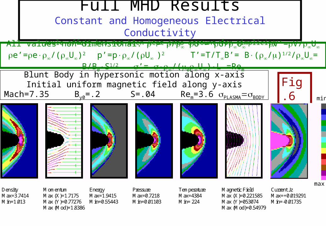
Full MHD ResultsConstant and Homogeneous Electrical Conductivity

Joule effect has not been kept into account for simplicity

Fig.6

All values non-dimensional: ’= / U’= U/U V’=V/U e’=e/(U)2

p’=p/(U )2 T’=T/TB’= B(/)1/2/U= B/B0S1/2 ’= /(0U)L =Rem

Blunt Body in hypersonic motion along x-axisInitial uniform magnetic field along y-axis

Mach=7.35 By0=.2 S=.04 Rem=3.6 PLASMABODY min

maxDensity Momentum Energy Pressure Temperature Magnetic Field Current JzMax=3.7414 Max (X)=1.7175 Max=1.9415 Max=0.7218 Max=4384 Max (X)=0.221585 Max=+0.019291Min=1.013 Max (Y)=0.77276 Min=0.55443 Min=0.01103 Min= 224 Max (Y)=053074 Min=-0.01735

Max (Mod)=1.8386 Max (Mod)=0.54979

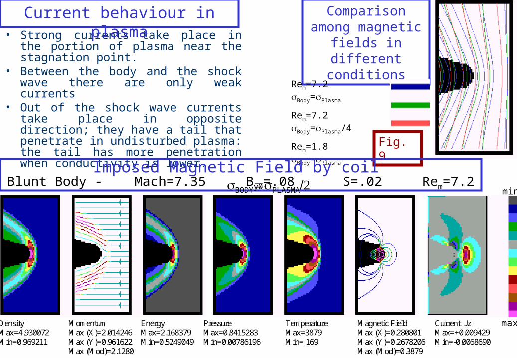
• Strong currents take place in the portion of plasma near the stagnation point.

• Between the body and the shock wave there are only weak currents

• Out of the shock wave currents take place in opposite direction; they have a tail that penetrate in undisturbed plasma: the tail has more penetration when conductivity is lower.

Current behaviour in plasma

Fig. 9

Comparison among magnetic fields in

different conditions

Rem=7.2 Body=Plasma

Rem=7.2 Body=Plasma/4

Rem=1.8 Body=Plasma

min

maxDensity Momentum Energy Pressure Temperature Magnetic Field Current JzMax=4.930072 Max (X)=2.014246 Max=2.168379 Max=0.8415283 Max=3879 Max (X)=0.280801 Max=+0.009429Min=0.969211 Max (Y)=0.961622 Min=0.5249049 Min=0.00786196 Min= 169 Max (Y)=0.2678206 Min=-0.0068690

Max (Mod)=2.1280 Max (Mod)=0.3879

Imposed Magnetic Field by coil Blunt Body - Mach=7.35 By0=.08 S=.02 Rem=7.2 BODYPLASMA

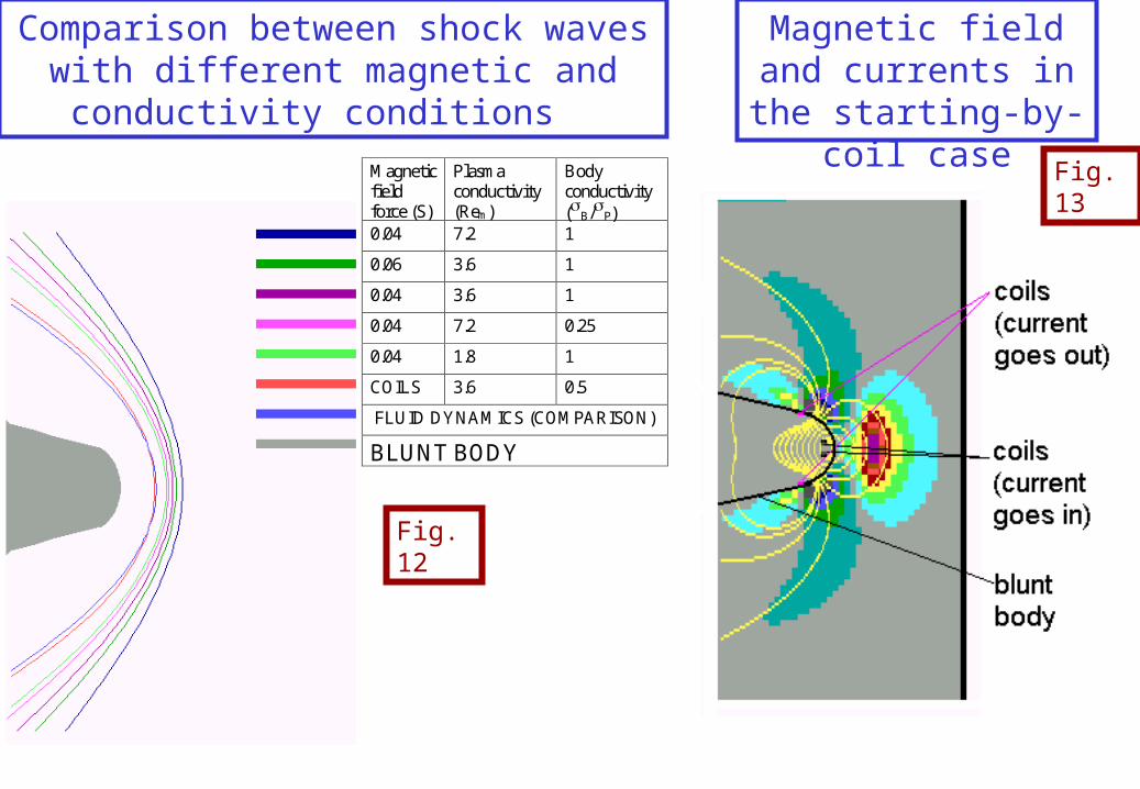
Comparison between shock waves with different magnetic and conductivity

conditions

Magneticfieldforce (S)

Plasmaconductivity(Rem)

Bodyconductivity(B/P)

0.04 7.2 1

0.06 3.6 1

0.04 3.6 1

0.04 7.2 0.25

0.04 1.8 1

COILS 3.6 0.5

FLUID DYNAMICS (COMPARISON)

BLUNT BODY

Magnetic field and currents in the starting-

by-coil case

Fig.13

Fig.12

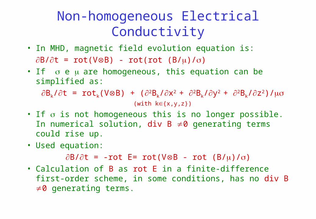
Non-homogeneous Electrical Conductivity

• In MHD, magnetic field evolution equation is:

B/t = rot(VB) - rot(rot (B/)/)

• If e are homogeneous, this equation can be simplified as:

Bk/t = rotk(VB) + (2Bk/x2 + 2Bk/y2 + 2Bk/z2)/(with k{x,y,z})

• If is not homogeneous this is no longer possible. In numerical solution, div B 0 generating terms could rise up.

• Used equation:

B/t = -rot E= rot(VB - rot (B/)/)

• Calculation of B as rot E in a finite-difference first-order scheme, in some conditions, has no div B 0 generating terms.

Low and Non-homogeneous Electrical Conductivity

• In scheme in which electrical conductivity is calculated by chemical reactions, usually the conductivity is initially zero, then firstly it rise up to low values, eventually it reaches significant values.

• In MHD, if electrical conductivity becomes zero, the rot (B/)/ term in magnetic field evolution equation diverges.

• To avoid these problems a very low artificial, homogeneous conductivity is imposed over all the scheme.

Low and Non-homogeneous Electrical Conductivity

• Problems:

- Artificial conductivity has to be low enough to not affect fluid dynamic scheme.

This is verified by comparison with a “frozen” magnetic field case.

- In case of very low electrical conductivity, time step has to be small enough to reach stability in the scheme → High calculation time.

Solution:

A) Very simple, high speed ad-hoc Maxwell solver implementation.

B) Double-time step implementation:

∆t Fluid Dynamics = 10 ÷100 ∆t Electromagnetics

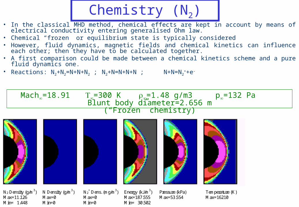
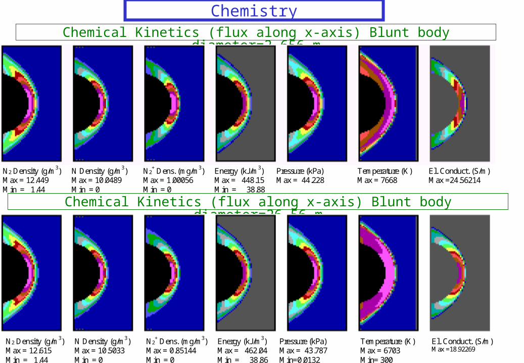
Chemistry (N2)

Mach=18.91=300 K =1.48 g/m3 p=132 Pa Blunt body diameter=2.656 m

(“Frozen” chemistry)

• In the classical MHD method, chemical effects are kept in account by means of electrical conductivity entering generalised Ohm law.

• Chemical “frozen” or equilibrium state is typically considered• However, fluid dynamics, magnetic fields and chemical kinetics can influence each other; then they

have to be calculated together.• A first comparison could be made between a chemical kinetics scheme and a pure fluid dynamics one.• Reactions: N2+N2=N+N+N2 ; N2+N=N+N+N ; N+N=N2

++e-

N2 Density (g/m3) N Density (g/m3) N2+ Dens. (mg/m3) Energy (kJ/m3) Pressure (kPa) Temperature (K)

Max=11.126 Max=0 Max=0 Max=187.555 Max=53.554 Max=16210Min= 1.448 Min=0 Min=0 Min= 30.502

ChemistryChemical Kinetics (flux along x-axis) Blunt body diameter=2.656 m

N2 Density (g/m3) N Density (g/m3) N2+ Dens. (mg/m3) Energy (kJ/m3) Pressure (kPa) Temperature (K)

Max=11.126 Max=0 Max=0 Max=187.555 Max=53.554 Max=16210Min= 1.448 Min=0 Min=0 Min= 30.502

N2 Density (g/m3) N Density (g/m3) N2+ Dens. (mg/m3) Energy (kJ/m3) Pressure (kPa) Temperature (K) El. Conduct. (S/m)

Max = 12.449 Max = 10.0489 Max = 1.00056 Max = 448.15 Max = 44.228 Max = 7668 Max =24.56214Min = 1.44 Min = 0 Min = 0 Min = 38.88

“Frozen” Chemistry

• Fluid Dynamics is high influenced by chemical reactions:- Chemical Reaction absorbs energy (Temperature goes down)

• Reactions velocity is influenced by body dimensions:- Small body:

-Low nitrogen dissociation;

-High temperature

-High ionization.

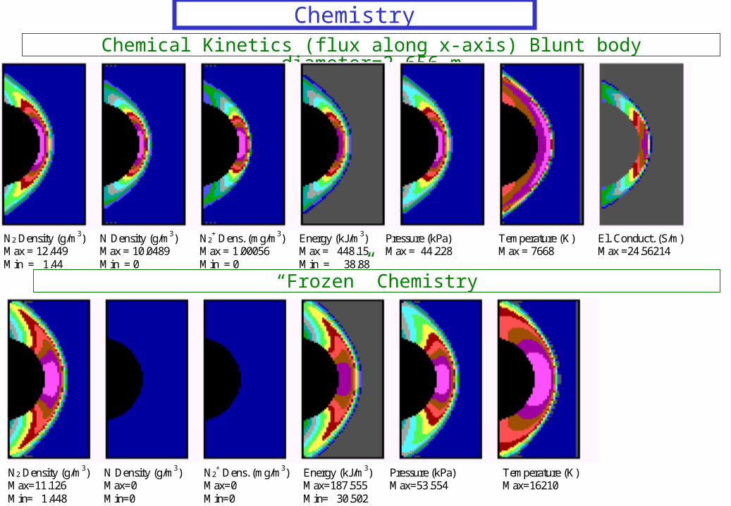
ChemistryChemical Kinetics (flux along x-axis) Blunt body diameter=2.656 m

N2 Density (g/m3) N Density (g/m3) N2+ Dens. (mg/m3) Energy (kJ/m3) Pressure (kPa) Temperature (K) El. Conduct. (S/m)

Max = 12.615 Max = 10.5033 Max = 0.85144 Max = 462.04 Max = 43.787 Max = 6703 Max =18.92269

Min = 1.44 Min = 0 Min = 0 Min = 38.86 Min=0.0132 Min= 300

N2 Density (g/m3) N Density (g/m3) N2+ Dens. (mg/m3) Energy (kJ/m3) Pressure (kPa) Temperature (K) El. Conduct. (S/m)

Max = 12.449 Max = 10.0489 Max = 1.00056 Max = 448.15 Max = 44.228 Max = 7668 Max =24.56214Min = 1.44 Min = 0 Min = 0 Min = 38.88

Chemical Kinetics (flux along x-axis) Blunt body diameter=26.56 m

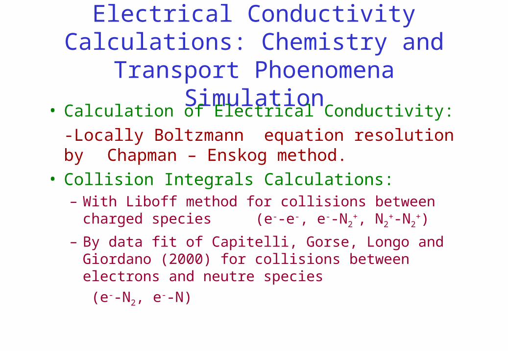
Electrical Conductivity Calculations: Chemistry and Transport Phoenomena

Simulation• Calculation of Electrical Conductivity:

-Locally Boltzmann equation resolution by Chapman – Enskog method.

• Collision Integrals Calculations:– With Liboff method for collisions between charged species

(e--e-, e--N2+, N2

+-N2+)

– By data fit of Capitelli, Gorse, Longo and Giordano (2000) for collisions between electrons and neutre species

(e--N2, e--N)

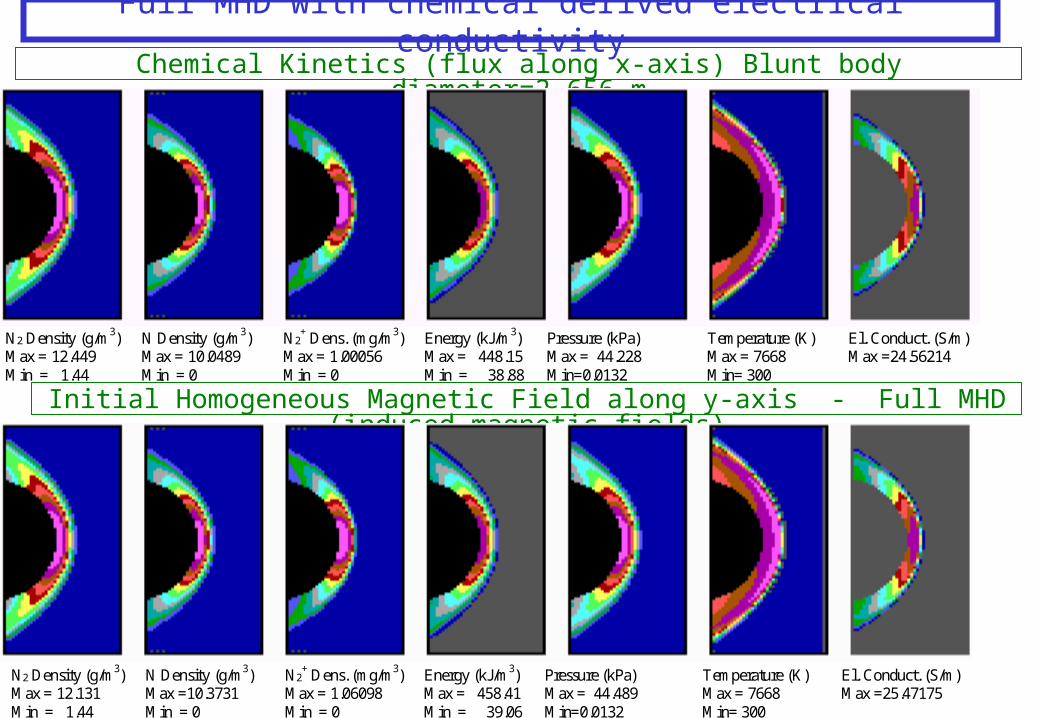
Full MHD with chemical derived electrical conductivityChemical Kinetics (flux along x-axis) Blunt body diameter=2.656 m

N2 Density (g/m3) N Density (g/m3) N2+ Dens. (mg/m3) Energy (kJ/m3) Pressure (kPa) Temperature (K) El. Conduct. (S/m)

Max = 12.131 Max =10.3731 Max = 1.06098 Max = 458.41 Max = 44.489 Max = 7668 Max =25.47175Min = 1.44 Min = 0 Min = 0 Min = 39.06 Min=0.0132 Min= 300

N2 Density (g/m3) N Density (g/m3) N2+ Dens. (mg/m3) Energy (kJ/m3) Pressure (kPa) Temperature (K) El. Conduct. (S/m)

Max = 12.449 Max = 10.0489 Max = 1.00056 Max = 448.15 Max = 44.228 Max = 7668 Max =24.56214Min = 1.44 Min = 0 Min = 0 Min = 38.88 Min=0.0132 Min= 300

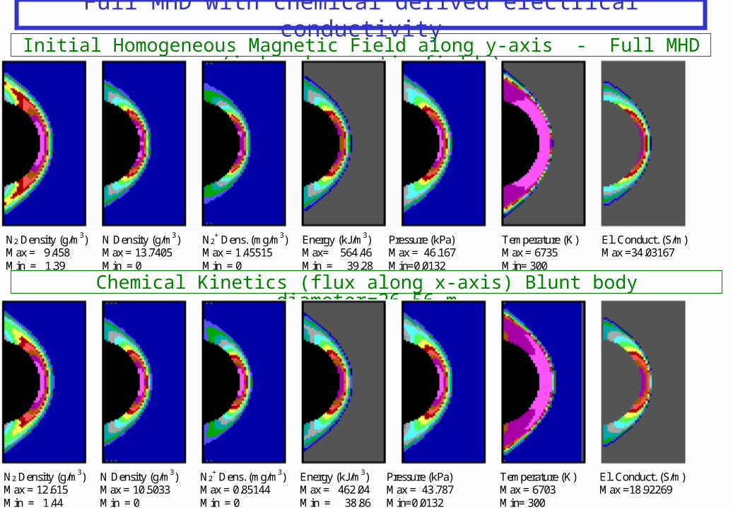
Initial Homogeneous Magnetic Field along y-axis - Full MHD (induced magnetic fields)

Full MHD with chemical derived electrical conductivity

Chemical Kinetics (flux along x-axis) Blunt body diameter=26.56 m

N2 Density (g/m3) N Density (g/m3) N2+ Dens. (mg/m3) Energy (kJ/m3) Pressure (kPa) Temperature (K) El. Conduct. (S/m)

Max = 9.458 Max = 13.7405 Max = 1.45515 Max= 564.46 Max = 46.167 Max = 6735 Max =34.03167Min = 1.39 Min = 0 Min = 0 Min = 39.28 Min=0.0132 Min= 300

N2 Density (g/m3) N Density (g/m3) N2+ Dens. (mg/m3) Energy (kJ/m3) Pressure (kPa) Temperature (K) El. Conduct. (S/m)

Max = 12.615 Max = 10.5033 Max = 0.85144 Max = 462.04 Max = 43.787 Max = 6703 Max =18.92269Min = 1.44 Min = 0 Min = 0 Min = 38.86 Min=0.0132 Min= 300

Initial Homogeneous Magnetic Field along y-axis - Full MHD (induced magnetic fields)

Profile comparison of total density (a) and pressure (b) along symmetry central line. Fluid dynamic + chemistry case data are plotted in solid line; Full MHD case data are plotted in dashed line

Comparison of density ratio and pressure contour plots:

• Fluid dynamic +chemistry (lower side)

• With Full MHD (upper side).

Comparison between magnetic field “frozen” case and full MHD case

Conclusions

• Fluid Dynamics, electromagnetism and chemical reactions have high influence each others

• Particularly, chemical reaction influence has been found.

• In other conditions this influence could be also higher.

Next Developements

• Influence of other transport parameters:

Thermical conductivity,Viscosity, Diffusion• Tensorial Electric Conductivity• Other Chemical Species (Oxygen): Complete air

chemistry.• Larger Mach number• Non-Homogeneous initial Magnetic Field (by coils)