Page 1
Portland State University Portland State University
PDXScholar PDXScholar
Dissertations and Theses Dissertations and Theses
1-1-2011
Numerical Modeling and Analyses of Steel Bridge Numerical Modeling and Analyses of Steel Bridge
Gusset Plate Connections Gusset Plate Connections
Thomas Sidney Kay Portland State University
Follow this and additional works at: https://pdxscholar.library.pdx.edu/open_access_etds
Let us know how access to this document benefits you.
Recommended Citation Recommended Citation Kay, Thomas Sidney, "Numerical Modeling and Analyses of Steel Bridge Gusset Plate Connections" (2011). Dissertations and Theses. Paper 84. https://doi.org/10.15760/etd.84
This Thesis is brought to you for free and open access. It has been accepted for inclusion in Dissertations and Theses by an authorized administrator of PDXScholar. Please contact us if we can make this document more accessible: [email protected] .
Page 2
Numerical Modeling and Analyses of Steel Bridge Gusset Plate Connections
by
Thomas Sidney Kay
A thesis submitted in partial fulfillment of the
requirements for the degree of
Master of Science
in
Civil and Environmental Engineering
Thesis Committee:
Peter Dusicka, Chair
Manouchehr Gorji
Hormoz Zareh
Portland State University
©2011
Page 3
i
Abstract
Gusset plate connections are commonly used in steel truss bridges to connect
individual members together at a node. Many of these bridges are classified as non-load-
path-redundant bridges, meaning a failure of a single truss member or connection could
lead to collapse. Current gusset plated design philosophy is based upon experimental
work from simplified, small-scale connections which are seldom representative of bridge
connections. This makes development of a refined methodology for conducting high-
fidelity strength capacity evaluations for existing bridge connections a highly desirable
goal. The primary goal of this research effort is to develop an analytical model capable
of evaluating gusset plate stresses and ultimate strength limit states. A connection-level
gusset connection model was developed in parallel with an experimental testing program
at Oregon State University. Data was collected on elastic stress distributions and ultimate
buckling capacity. The analytical model compared different bolt modeling techniques on
their effectiveness in predicting buckling loads and stress distributions. Analytical tensile
capacity was compared to the current bridge gusset plate design equations for block
shear. Results from the elastic stress analysis showed no significant differences between
the bolt modeling techniques examined, and moderate correlation between analytical and
experimental values. Results from the analytical model predicted experimental buckling
capacity within 10% for most of the bolt modeling techniques examined. Tensile
capacity was within 7% of the calculated tensile nominal capacity for all bolt modeling
techniques examined. A preliminary parametric study was conducted to investigate the
effects of member flexural stiffness and length on gusset plate buckling capacity, and
Page 4
ii
showed an increase in member length or decrease in member flexural stiffness resulted in
diminished gusset plate buckling capacity.
Page 5
iii
Dedication
To my wife Kimberly, thank you for all of your love, support and patience. You
have been a great source of inspiration and strength for me during my academic pursuits.
To my mother Sara, thank you for believing in my abilities and helping me along every
step of the way. To my son Henry, thank you for being the best part of my day, every
day and showing me the love and wonderment of childhood.
Page 6
iv
Acknowledgements
I would like to thank my mentor Dr. Dusicka for taking me on as a graduate
student and research assistant in the iSTAR laboratory. Your guidance and high
standards for excellence have helped me become a better engineer and researcher, and for
that I am grateful.
I would also like to thank my other committee members Dr. Zareh and Dr. Gorji.
Your courses proved to be some of the most challenging and the most rewarding. You
both have instilled a lasting impression on me and I owe you my thanks.
Page 7
v
Table of Contents
Abstract ................................................................................................................................ i
Dedication .......................................................................................................................... iii
Acknowledgements ............................................................................................................ iv
List of Tables .................................................................................................................... vii
List of Figures .................................................................................................................. viii
1.0 Introduction ................................................................................................................... 1
1.1 Overview ................................................................................................................... 1
1.2 Objectives .................................................................................................................. 3
1.3 Scope ......................................................................................................................... 4
2.0 Literature Review.......................................................................................................... 5
2.1 Elastic Behavior of Gusset Plates.............................................................................. 5
2.2 Gusset Plate Failure States in Tension ...................................................................... 7
2.3 Gusset Plate Failure States in Compression .............................................................. 9
2.4 Past Bridge Gusset Plate Failures ........................................................................... 11
2.4.1 Grand River Bridge Gusset Plate Failure (Lake County, Ohio) ....................... 12
2.4.2 I-35W Bridge Gusset Plate Failure (Minneapolis, MN) ................................... 13
2.5 Gusset Plate Load Rating Methods According to FHWA ...................................... 14
2.6 Previous FEA Gusset Plate Models ........................................................................ 17
2.7 Summary ................................................................................................................. 19
3.0 Numerical Modeling ................................................................................................... 21
3.1 Objectives ................................................................................................................ 21
3.2 Fastener Modeling ................................................................................................... 21
3.2.1 Beam Element Bolt Models .............................................................................. 22
3.2.2 Three-Dimensional Contact Bolt Models ......................................................... 23
3.2.3 Radial-Spring (RS) Bolt Model ........................................................................ 24
3.3 Single Bolt Connection Model ................................................................................ 25
3.3.1 Single Bolt Connection Model - Results and Discussion ................................. 28
3.4 Multi-Bolt Connection Model ................................................................................. 29
3.4.1 Sample A - Results and Discussion .................................................................. 30
3.4.2 Sample B - Results and Discussion .................................................................. 31
3.4.3 Summary ........................................................................................................... 32
3.5 Gusset Connection Model Description ................................................................... 32
Page 8
vi
3.5.1 Material Modeling ............................................................................................ 34
3.5.2 Element Selection ............................................................................................. 35
3.5.3 Mesh Refinement .............................................................................................. 35
3.5.3 Elastic Stress Analysis ...................................................................................... 36
3.5.4 Buckling Capacity Analysis ............................................................................. 37
3.5.5 Tensile Capacity Analysis ................................................................................ 40
3.6 Gusset Connection Experimental Program (Oregon State)..................................... 40
3.6.1 Test 1 – Description and Results ...................................................................... 40
3.6.2 Test 2 – Description and Results ...................................................................... 43
3.6.3 Test 3 – Description and Results ...................................................................... 44
3.7 Analytical Results and Experimental Validation .................................................... 44
3.7.1 Elastic Stresses ................................................................................................. 44
3.7.2 Buckling Capacity ............................................................................................ 47
3.7.3 Tensile Capacity ............................................................................................... 48
3.8 Conclusions and Modeling Recommendations ....................................................... 49
4.0 Parametric Study ......................................................................................................... 52
4.1 Effects of plate thickness and imperfection ............................................................ 53
4.2 Effects of adjustment of Whitmore’s effective length ............................................ 54
4.3 Effects of connected member flexural stiffness and length .................................... 55
4.4 Summary and Conclusion ....................................................................................... 56
5.0 Conclusions and Recommendations for Further Study .............................................. 58
Tables ................................................................................................................................ 61
Figures............................................................................................................................... 65
References ....................................................................................................................... 101
Appendix A – Capacity and Design Calculations ........................................................... 104
Appendix B – Python Scripts .......................................................................................... 111
Multi-bolt connection model script – RS bolts ........................................................... 111
Gusset connection model script – RS Bolts ................................................................ 118
Appendix C – Convergence plots ................................................................................... 130
Page 9
vii
List of Tables
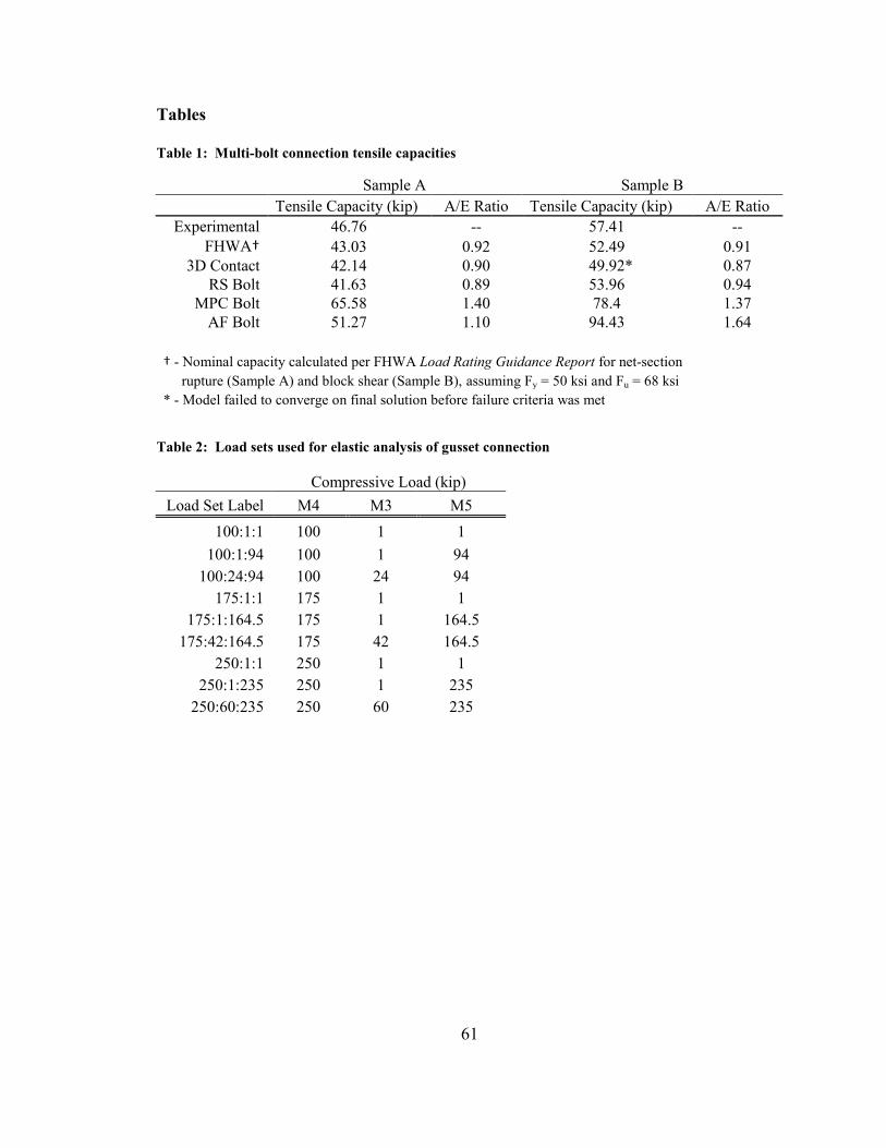
Table 1: Multi-bolt connection tensile capacities ............................................................ 61
Table 2: Load sets used for elastic analysis of gusset connection ................................... 61
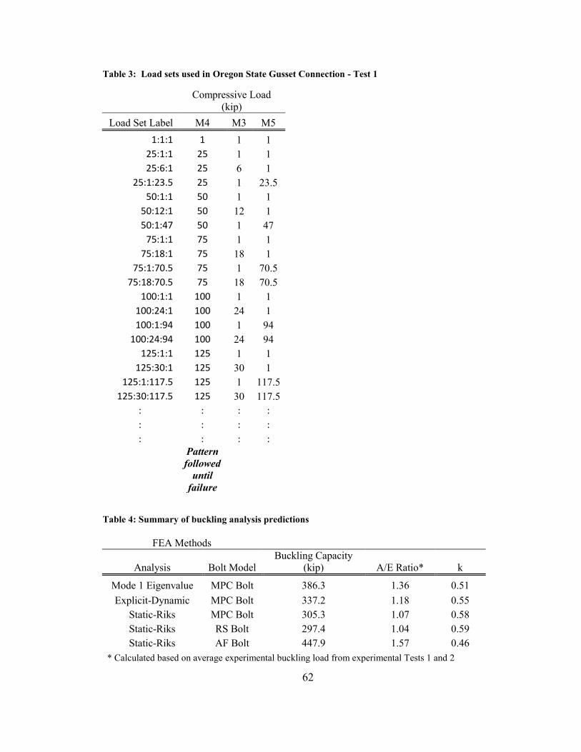
Table 3: Load sets used in Oregon State Gusset Connection - Test 1 ............................. 62
Table 4: Summary of buckling analysis predictions ......................................................... 62
Table 5: Summary of tensile capacity predictions ........................................................... 63
Table 6: Buckling capacity and k values due to imperfections ......................................... 63
Table 7: Buckling capacity and k values for different gusset plate effective lengths ...... 63
Table 8: Buckling capacity and k values for different member flexural stiffnesses ........ 64
Table 9: Buckling capacity and k values for different M4 lengths .................................. 64
Page 10
viii
List of Figures
Figure 1: Warren truss gusset plate connection tested by Whitmore (1957) ................... 65
Figure 2: Whitmore effective width definitions for member regions of gusset plates
(NTSB, 2008) .................................................................................................................... 65
Figure 3: Pratt truss gusset plate tested by Irvin and Hardin ........................................... 66
Figure 4: Gusset plate connection tested by Bjorhovde and Chakrabarti (1985) ............ 66
Figure 5: General gusset plates tested by Hardash and Bjorjovde (1985) ....................... 67
Figure 6: Whitmore effective length definitions (NTSB, 2008) ...................................... 67
Figure 7: Test frame and gusset plate connection (Yamamoto, 1988) ............................ 68
Figure 8: Gusset plate test specimen assembly (Gross, 1990) ......................................... 69
Figure 9: Gusset plate failure on the Lake County Grand River Bridge, Ohio ............... 69
Figure 10: (a) U10 gusset connection, (b) free edge distortion in 2003 ........................... 70
Figure 11: Post-collapse investigation photo of U10 connection, I35-W Bridge,
Minneapolis MN ............................................................................................................... 71
Figure 12: Radial Spring (RS) Bolt Model ...................................................................... 71
Figure 13: Single bolt model, (a) 3D contact bolt, (b) radial spring bolt ........................ 72
Figure 14: Load-displacement curves for different number of radial springs used .......... 72
Figure 15: Local mesh convergence for RS bolt model .................................................. 73
Figure 16: PEEQ contours for different bolt modeling methods ..................................... 74
Figure 17: Load-displacement behavior for single-bolt models ...................................... 75
Figure 18: Test setup schematic and drawings for Samples A and B. ............................. 75
Figure 19: Displacement measurement instrumentation for multi-bolt tests ................... 76
Figure 20: True stress-strain properties for gusset plate material property definition ..... 76
Figure 21: PEEQ contours for multi-bolt models for Sample A ..................................... 77
Figure 22: Load-displacement behavior for Sample A .................................................... 77
Figure 23: PEEQ contours for Sample B ......................................................................... 78
Figure 24: Load-displacement behavior for Sample B .................................................... 78
Figure 25: Gusset plate connection; (a) experimental setup, (b) FEA model ................... 79
Figure 26: Gusset connection member modeling ............................................................ 80
Figure 27: Boundary conditions and actuator load capacities for gusset plate connection
........................................................................................................................................... 80
Figure 28: Stress planes and sample points used for elastic stress analysis .................... 81
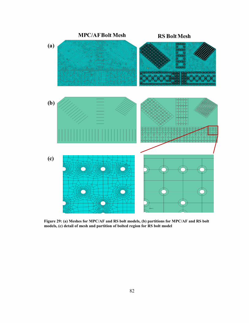
Figure 29: (a) Meshes for MPC/AF and RS bolt models, (b) partitions for MPC/AF and
RS bolt models, (c) detail of mesh and partition of bolted region for RS bolt model ...... 82
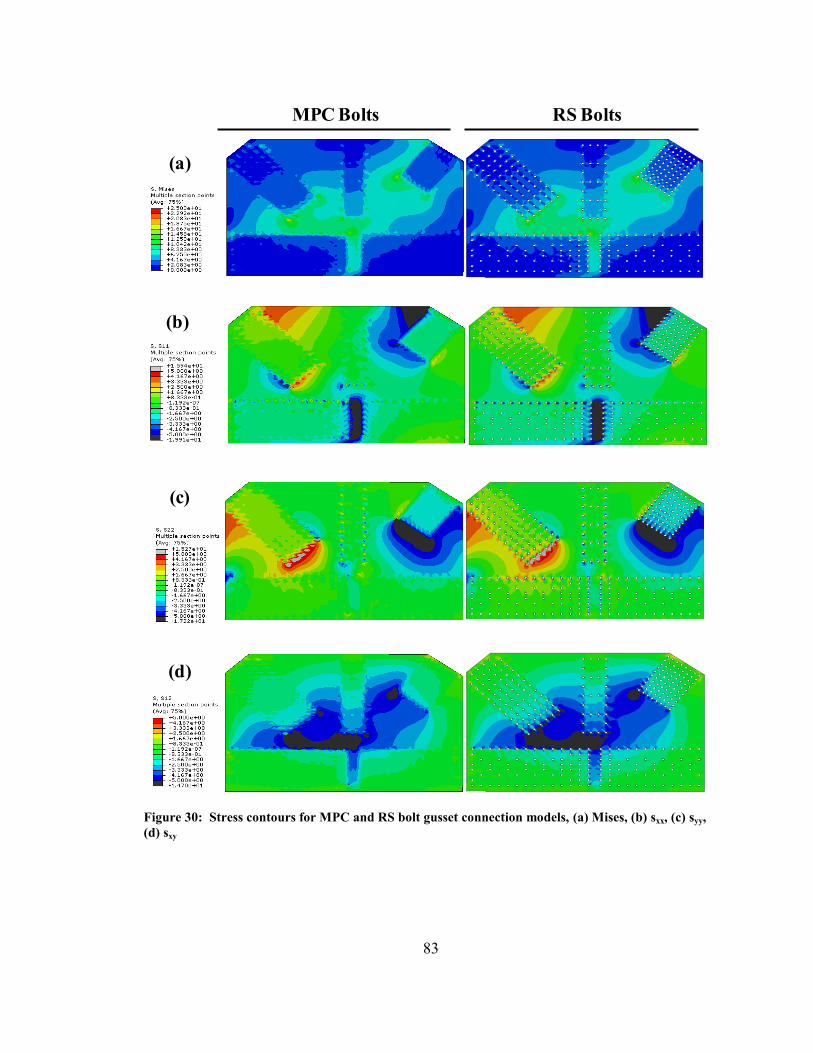
Figure 30: Stress contours for MPC and RS bolt gusset connection models, (a) Mises, (b)
sxx, (c) syy, (d) sxy ............................................................................................................... 83
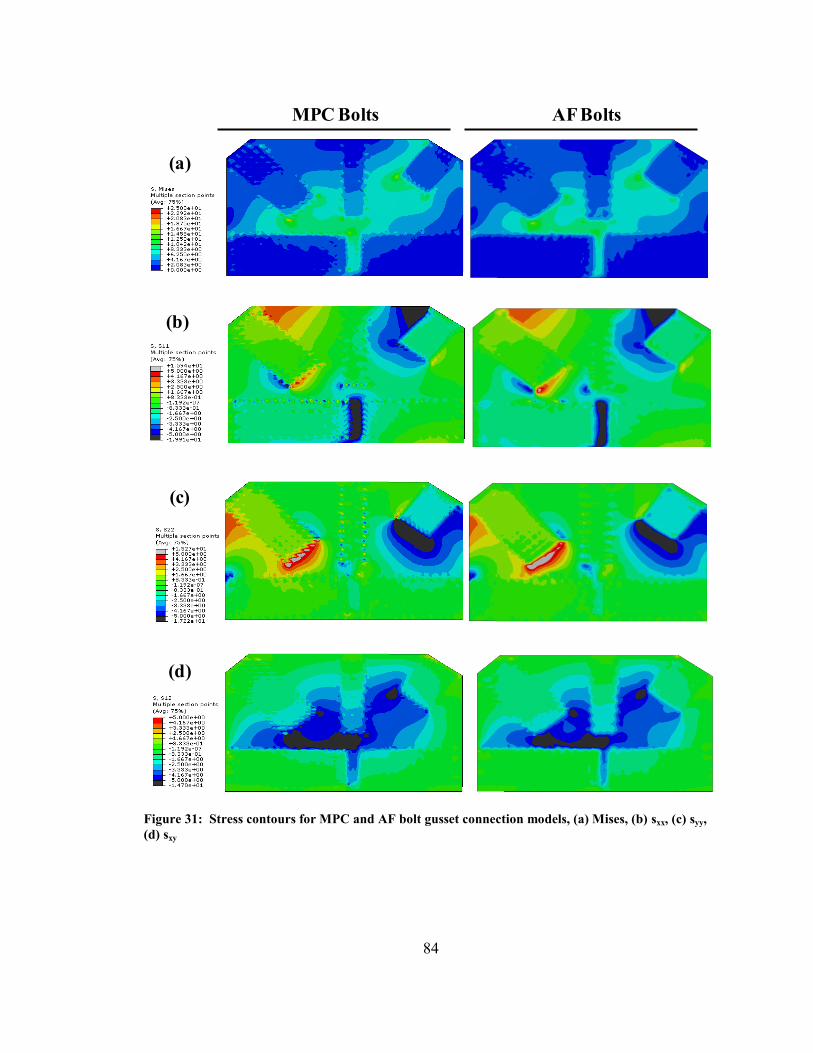
Figure 31: Stress contours for MPC and AF bolt gusset connection models, (a) Mises, (b)
sxx, (c) syy, (d) sxy ............................................................................................................... 84
Figure 32: Plane A stress profiles for MPC, AF and RS bolt models ............................. 85
Page 11
ix
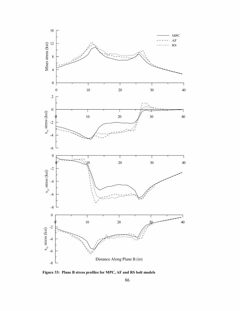
Figure 33: Plane B stress profiles for MPC, AF and RS bolt models .............................. 86
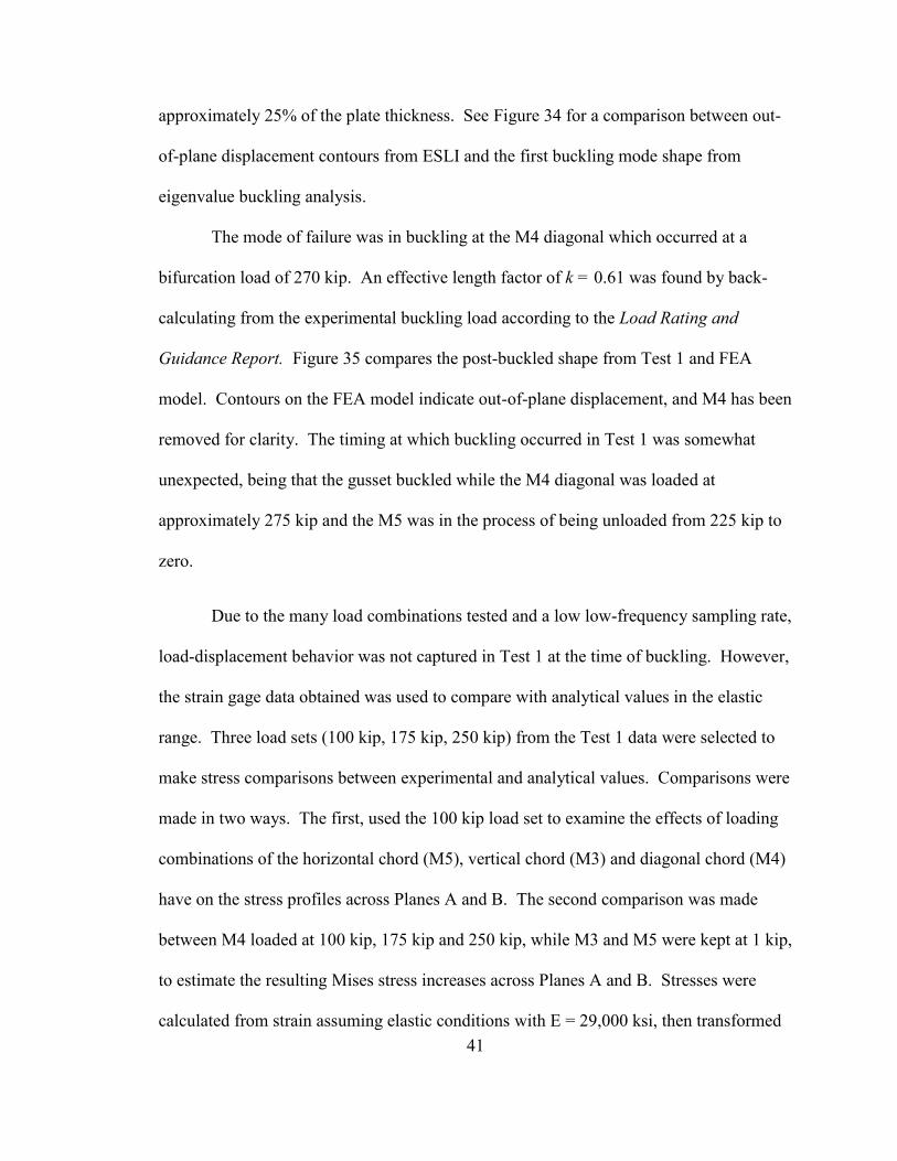
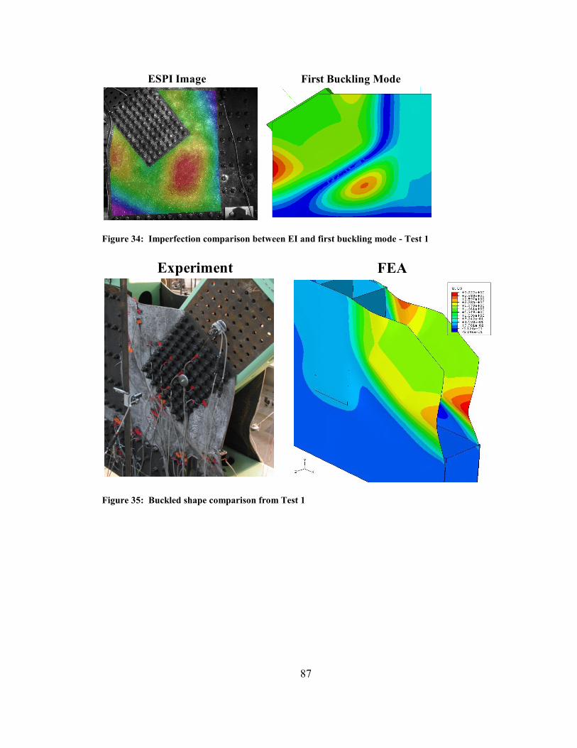
Figure 34: Imperfection comparison between EI and first buckling mode - Test 1 ........ 87
Figure 35: Buckled shape comparison from Test 1 ......................................................... 87
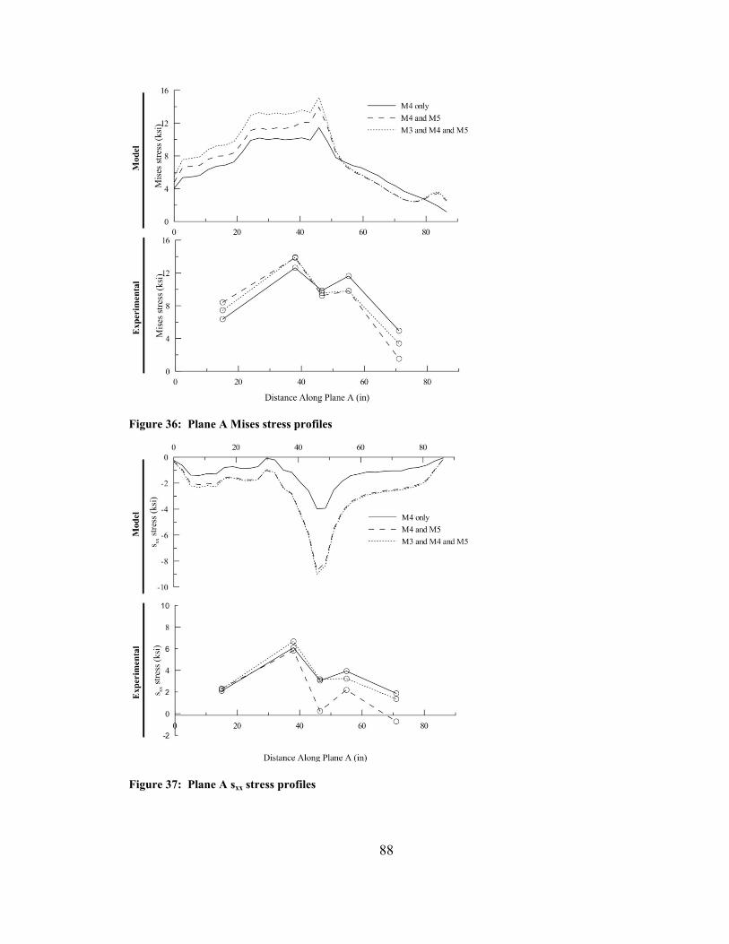
Figure 36: Plane A Mises stress profiles.......................................................................... 88
Figure 37: Plane A sxx stress profiles ............................................................................... 88
Figure 38: Plane A syy stress profiles ............................................................................... 89
Figure 39: Plane A sxy stress profiles ............................................................................... 89
Figure 40: Plane B Mises stress profiles .......................................................................... 90
Figure 41: Plane B sxx stress profiles ............................................................................... 90
Figure 42: Plane B syy stress profiles ............................................................................... 91
Figure 43: Plane B sxy stress profiles ............................................................................... 91
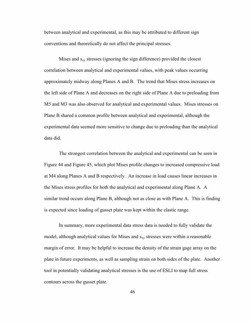
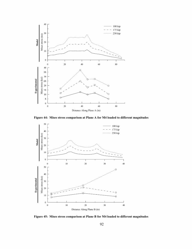
Figure 44: Mises stress comparison at Plane A for M4 loaded to different magnitudes . 92
Figure 45: Mises stress comparison at Plane B for M4 loaded to different magnitudes . 92
Figure 46: Measurements used to construct gusset connection load-displacement plots 93
Figure 47: Compression load-displacement comparisons between MPC, AF and RS bolt
models with experimental ................................................................................................. 93
Figure 48: Compression load-displacement comparisons between analysis methods and
experimental ...................................................................................................................... 94
Figure 49: Buckled gusset connection - Test 2 ................................................................ 94
Figure 50: buckled gusset connection - Test 3 ................................................................. 95
Figure 51: Tensile load-displacement curves for gusset connection ............................... 95
Figure 52: Mises and PEEQ contour comparisons from tensile failure analysis for MPC,
AF and MPC bolt models ................................................................................................. 96
Figure 53: Mises stress contour detail for RS bolt model ................................................ 97
Figure 54: Load-displacement curves for 1/4" plate and varying out-of-plane
imperfection ...................................................................................................................... 98
Figure 55: k vs. degree of initial imperfection .................................................................. 98
Figure 56: Load-displacement curves for different Whitmore effective lengths ............. 99
Figure 57: Buckling capacity vs. Whitmore effective length .......................................... 99
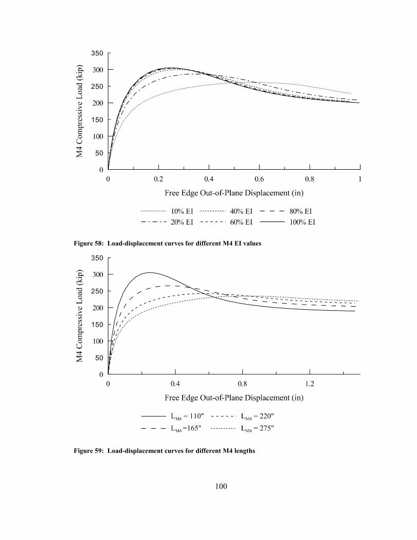
Figure 58: Load-displacement curves for different M4 EI values ................................. 100
Figure 59: Load-displacement curves for different M4 lengths .................................... 100
Page 12
1
1.0 Introduction
1.1 Overview
Gusset plate connections are commonly used in steel truss bridges to connect
individual members together at a node. The connection typically consists of a steel plate
on each side of the connected members, then bolted or riveted together. A large number
of steel deck truss bridges are currently in service. The Federal Highway Administration
estimates that 465 steel deck truss bridges and approximately 11,000 deck truss bridges
exist in the National Bridge Inventory (NTSB, 2008). Many of these bridges are further
classified as non-load-path-redundant bridges meaning a failure of a single truss member
or connection could lead to collapse. This makes periodic inspections and load rating
practices essential for the safe operation and maintenance of these bridge types.
Historically, only the truss members were evaluated for load capacity. The
rationale for omitting load rating for connections comes from what is thought to be
conservative assumptions employed during connection design, combined with a small
occurrences of connection failures in the historical record; namely the 1996 gusset plate
failure on the Grand River Bridge in Lake County, Ohio (NTSB, 2008) (NTSB, 2008)
(NTSB, 2008), and the 2007 collapse of the I-35W Bridge in Minneapolis, Minnesota
(Holt & Hartmann, 2008). The collapse of the I-35 Bridge in Minneapolis was
catastrophic – resulting in 13 deaths and 145 injuries – and was the first failure where a
design error was implicated as the cause of collapse, thus revealing a new vulnerability in
steel truss bridges which had previously been thought to be both economical and reliable.
Page 13
2
After the I-35W Bridge collapse, the Federal Highway Association (FHWA) issued a set
of guidelines for load rating gusset plate connections (FHWA, 2009), yet did not provide
any revised design methods beyond existing practice. Instead, a summary was compiled
of existing design methods and load rating procedures for gusset plate connections.
Inclusion of gusset plate connections in load ratings poses a significant challenge
to bridge owners due to the large number of connections in the inventory and the
complexity of analysis required to accurately evaluate each connection. Load transfer to
bridge gusset plates in situ is delivered by multiple members – all potentially with axial,
shear and moment – through the fasteners into bearing on the gusset plate. However,
current gusset plate design philosophy is rooted in elementary beam theory analysis and
applicable specification rules, combined with the experience and judgment of the
designer (Bjorhovde & Chakrabarti, 1985). Moreover, current design philosophy is
based upon experimental work done on small-scale gusset connections consisting of a
single braced member acting in monotonic axial tension or compression; which is hardly
representative of bridge connections. The complexity of stress fields and failure states
found in gusset plates is addressed by applying approximate methods to arrive at a rapid,
albeit conservative solution, but one that may lack accuracy. Thus, development of a
refined methodology for conducting high-fidelity strength capacity evaluations on
existing bridge connections is a highly desirable goal.
Toward this end, finite element analysis (FEA) is an appealing option for
analyzing stresses and failure states of bridge gusset plate connections. FEA is widely
used in structural engineering applications, with modern commercial software packages
Page 14
3
capable of modeling systems with non-linear material behavior, complex geometry,
contact interactions and complex loading conditions. FEA implementation in bridge
connection evaluations does present some challenges due to the large scale, high degree
of geometric variability and complex load paths that are unique for each connection.
Sophisticated non-linear FEA models may be well suited for evaluating strength
capacities in bridge connections, but have yet to be calibrated with experimental results
from large-scale experiments. Nor is there consensus among practitioners regarding how
complex a FEA model must be to accurately capture a connection’s ultimate strength
capacity. Complex FEA modeling involves significant development time, specialized
training, and often comes at the cost of long computation times. This consequently
translates into significant cost for bridge owners, and can delay the incorporation of
connection load rating into bridge inspection programs.
1.2 Objectives
The impetus for this work arises from the need for accurate and rapid assessment
of bridge connections, a re-evaluation of existing design methods and a desire to better
understand the parameters affecting the strength capacity of bridge gusset plate
connections.
The objectives of this research are as follows:
1. Develop a FEA model, calibrated with experimental tests conducted at Oregon
State University, capable of evaluating gusset plate stresses and ultimate strength
limit states.
Page 15
4
2. Evaluate FEA modeling techniques for computational efficiency and ability to
predict ultimate strength capacity of bridge gusset plate connections subject to
tension and compression.
3. Conduct a parametric study to find the effects of initial imperfections, gusset plate
thickness, gusset plate effective length, member flexural stiffness and member
length on gusset plate buckling capacity.
4. Design the model to accept future modifications such as plate geometry, loading
conditions, boundary conditions, and fastener load-displacement behavior for
subsequent studies.
1.3 Scope
This work focuses on connection-level analysis of bridge gusset plates. Global
models of full bridge truss systems are not considered here, although they have been used
by others to study loading demands on particular connections. Only one bridge
connection geometry will be included in this study, which is from the specimen being
tested in a parallel experimental study at Oregon State University. Also, since the
primary research focus is on stresses and failure states of the gusset plates themselves,
attached members and fasteners will be modeled such that failure will only occur in the
gusset plate. Therefore, fastener and member failure states will not be considered in this
study.
Page 16
5
2.0 Literature Review
2.1 Elastic Behavior of Gusset Plates
Modern gusset plate design has been most influenced by Whitmore (1952), who
studied the stress distributions in a 1/4 scale model of a bottom chord Warren truss gusset
plate connection, similar to the one shown in Figure 1. Prior to Whitmore, gusset plate
design consisted of sizing the plate to accommodate the required number of fasteners,
then selecting a plate thickness based on classical beam formula analysis and engineering
judgment. Whitmore’s recognized that the use of beam theory was questionable, since
gusset plates act like deep members. He aimed to characterize the stress distribution in a
gusset plate subject to load, the magnitude and location of maximum stress, and develop
a simplified design method for determining maximum stresses in a gusset plate. The
experimental loading regime was kept in the elastic range of the gusset plate and was
applied such that one diagonal member was in tension, the other diagonal member was in
compression and the bottom chord was in tension. Stresses were calculated from an array
of strain gages positioned across the plate.
Whitmore’s findings showed that maximum stresses normal to the diagonals
occurred near the ends of the compression and tension diagonals respectively. Maximum
shear stress occurred along a plane just above the bottom chord and below the diagonal
members. Based on his findings, he proposed a simplified method for calculating
maximum normal stresses in a gusset plate, by using what has become known as the
Whitmore effective width (Figure 2). The Whitmore effective width is defined as the
length of the line perpendicular to the member axis passing through the last bolt row of
fasteners, intersected by two 30-degree lines drawn from the first outer row of fasteners
Page 17
6
to the last row. Maximum normal stress is calculated by multiplying the material’s yield
stress by the Whitmore effective width times the plate thickness. This technique for
calculating maximum normal stress in a gusset plate continues to be a fundamental rule in
gusset plate design.
Two studies by Irvin (1957) and Hardin (1958) expanded on Whitmore’s work
using a scale model of a bottom chord of a Pratt truss gusset plate connection shown in
Figure 3. Irvin’s findings supported Whitmore’s in regards to the location of maximum
tensile, compressive and shear stresses in the gusset plate occurred at the ends of the
compression, tension and plane above the horizontal chord. However, Irvin proposed an
alteration to the Whitmore effective width concept by drawing the two 30 degree lines
from the bolt group’s center of gravity to the last bolt row, as opposed to the outer gage
lines, resulting in a narrower effective width. Research by Hardin corroborated Irvin’s
results and recommendations.
Davis (1967) and Vasarhelyi (1971) were the first to use finite element analysis
methods to investigate stress distributions in gusset plates. Davis was the first to
replicate Whitmore’s findings analytically. Vasarhelyi conducted both experimental tests
and finite element analysis on a half-scale Warren truss with similar geometry to
Whitmore’s test specimen. Vasarhelyi also found that Whitmore’s approximate methods
were suitable for calculating the magnitude of maximum stresses, however the location of
maximum stresses may differ depending on how the connection is loaded.
Yamamoto (1986) reported on elastic stress distributions in full-scale Warren
truss and Pratt truss gusset plate connections, obtained from tests conducted for the
Honshu-Shikoku Bridge Authority in Japan. Yamamoto found that Whitmore’s methods
Page 18
7
were adequate for predicting maximum stress magnitudes, but the locations of the
maximum stresses can shift depending on the global loading condition of the connection,
specifically whether the bottom chord is loaded in tension or compression. This finding
is in agreement with Vasarhelyi (1971).
2.2 Gusset Plate Failure States in Tension
Due to the large scale and complexity involved in testing bridge connections,
most research investigating gusset plate failure states is confined to either small-scale
bridge truss connections, or simple connections found in lateral bracing systems for
buildings. Thornton (1984) presented a design methodology for all components of a
lateral bracing connection common to buildings, including gusset plates. The design
approach is based upon equilibrium, material yielding requirements and stiffness to
address buckling and fracture resistance. It is assumed that gusset plate tensile capacity
is governed by tear-out of the gusset plate – a failure mode analogous to the block shear –
where the sum of the net tensile and shear section strengths are calculated assuming bolt
diameter plus 1/16 ” hole allowance.
Bjorhovde and Chakrabarti (1985) tested 6 gusset plate connections under
tension, similar to the connection shown in Figure 4. The test matrix included two plate
thicknesses and three different bracing member orientation angles. For all samples, the
gusset plate failed by tensile rupture along the last row of bolts of the bracing member.
Further tearing occurred with samples where the Whitmore section intersected the edges
of the gusset plate. Work by Hardash and Bjorhovde (1985) also focused on gusset plate
tensile failures. Using samples like the one shown in Figure 5, block shear failure state
was examined in detail. The experimental program was designed to look at the effects of
Page 19
8
connection length, distance between outside bolt lines, plate thickness, bolt diameter,
material yield, and plate geometry on the plate’s tensile strength capacity. A total of 42
samples were tested, all of which failed in block shear with the same characteristic failure
progression; net tensile rupture at the last row of fasteners followed by various stages of
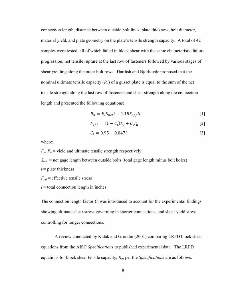
shear yielding along the outer bolt rows. Hardish and Bjorhovde proposed that the
nominal ultimate tensile capacity (Rn) of a gusset plate is equal to the sum of the net
tensile strength along the last row of fasteners and shear strength along the connection
length and presented the following equations:
[1]
[2]
[3]
where:
Fy, Fu = yield and ultimate tensile strength respectively
Snet = net gage length between outside bolts (total gage length minus bolt holes)
t = plate thickness
Feff = effective tensile stress
l = total connection length in inches
The connection length factor Ct was introduced to account for the experimental findings
showing ultimate shear stress governing in shorter connections, and shear yield stress
controlling for longer connections.
A review conducted by Kulak and Grondin (2001) comparing LRFD block shear
equations from the AISC Specifications to published experimental data. The LRFD
equations for block shear tensile capacity, Rn, per the Specifications are as follows:
Page 20
9
[4]
where:
Agv = gross area subject to shear
Ant = net area subject to tension
Anv = net area subject to shear
Ubs = 1.0 for gusset plates
Kulak found Equation [4] gave overly conservative predictions of gusset plate capacity,
and did not reflect the observed failure mode progression seen in experimental tests. The
reason is because the shear resistance is assumed to be 0.6 times the tensile strength,
therefore assuming the tension surface has adequate ductility to develop the full capacity
along the shear planes, an assumption that is in opposition to experimental evidence.
Therefore, Kulak recommended the equations presented by Hardish and Bjorhovde be
used for a better estimate of gusset plate tensile capacity.
2.3 Gusset Plate Failure States in Compression
The primary failure mode of gusset plates in compression is buckling. According
to Thornton (1984), compressive capacity can be calculated by considering the gusset
plate as an idealized column with a width of unity along the brace’s line of action and
length from the end of the Whitmore section to the plate edge, similar to that shown as L2
in Figure 6. The slenderness ratio kL/r is calculated assuming a fixed-fixed boundary
conditions with an effective length factor of k = 0.65. Alternatively, one can use the
average of L1, L2 and L3 for the section length, provided it does not produce a length
greater than L2. Thornton asserted that this is a conservative design approach since both
plate action and the gusset’s post-buckling strength is ignored.
Page 21
10
Hu and Cheng (1987) conducted experimental tests on gusset plate buckling
capacity in a simple braced frame connection; considering effects of gusset plate
thickness, boundary conditions, eccentricity and edge stiffening reinforcement. Thin
gusset plates were found to buckle at loads significantly lower than those predicted using
Whitmore’s effective width approach. Load at bifurcation was also shown to be highly
dependent on boundary conditions (sway and non-sway conditions were tested), plate
thickness and whether edge stiffeners were used. Yam and Cheng (1993) conducted a
follow-up investigation testing similar connections in compression. The test matrix
included varied plate thicknesses, plate size, brace angle orientation, and other variations
of the framing members. Yam and Cheng reported that the gusset plate’s compressive
capacity was almost directly proportional to plate thickness as well as dependent on sway
versus non-sway boundary conditions. They also proposed modifying the angle used to
the Whitmore effective width definition from 30 to 45 degrees to more accurately
account for the high degree of plate yielding and subsequent load re-distribution that
occurs pre-buckling.
Yamamoto (1988) published testing results on the buckling strength of full-scale
gusset plate bridge connections similar to those from his previous study on elastic stress
distributions. The loading truss used along with a representative test specimen is shown
in Figure 7. Experimental results were compared to the calculated design buckling
strength per guidelines by the Japan Society of Civil Engineers (JSCE, 1976). All the
connections failed because of highly localized buckling surrounding the compression
diagonal at loads approximately 2.5 to 3.7 times their design compression capacity. Of
note, the paper makes no discussion about the boundary conditions imposed on the
Page 22
11
connection, although photographs of the failed samples suggest a high degree of out-of-
plane constraint was present due to the short length of the members and the presence of
large end plates and stiffeners at the member ends.
Gross (1990) conducted experiments on gusset plate connections for a typical
building lateral bracing system. The test specimens included a top and bottom gusset
plate on either side of a beam framed into a column subassembly (Figure 8). Parameters
of interest were bracing member eccentricity relative to the beam to column working
point intersect, and whether a strong or weak-axis column alignment was included in the
subassembly. The subassembly was loaded laterally across the two top pins, inducing
tension in the top diagonal member and compression in the bottom diagonal member.
Two of the three samples tested failed by buckling of the bottom gusset plate, with the
third sample failing in block shear in the top gusset plate. Gross found that calculating
the gusset plate buckling capacity per AISC Engineering for Steel Construction (1984),
yielded values close to the experimental, provided that using an effective length factor of
k = 0.5 instead of Thornton’s k = 0.65. By decreasing the effective length factor, the
calculated compressive capacity is increased, hence accounting for additional strength
from post-buckling and plate action in the gusset plate.
2.4 Past Bridge Gusset Plate Failures
Only two known cases of gusset plate failures by the author exist on record in the
United States; namely the 1996 gusset plate failure on the Grand River Bridge in Lake
County, Ohio (NTSB, 2008) (NTSB, 2008) (NTSB, 2008) and the 2007 collapse of the I-
35W Bridge in Minneapolis, Minnesota. They are illustrative in demonstrating that the
Page 23
12
possibility that gusset failure is a continuing risk that can be sudden and catastrophic.
Below is a brief summary of findings from the forensic investigations.
2.4.1 Grand River Bridge Gusset Plate Failure (Lake County, Ohio)
The Lake County Grand River Bridges were twin bridges located about 30 miles
east of Cleveland, Ohio. Classified as steel deck truss bridges, each bridge consisted of 5
spans and carried two lanes of traffic in each direction for Interstate 90. Spans #1 and #5
were simply supported approaches; spans #2 and #4 were cantilevered deck trusses that
supported a suspended truss at span #5. The bridge was designed in 1958 and opened to
traffic in 1960.
According to a NTSB Factual Report on Ohio Bridges (2008), on May 24, 1996,
the eastbound bridge experienced a gusset plate buckling failure during a repainting
project, shown in Figure 9. One of the two lanes was closed to traffic during work.
Failure was supposedly initiated by vehicles and equipment involved with the repainting
project positioned over the failed node, combined with an overloaded truck crossing in
the open traffic lane. The gusset plate failure did not cause total collapse of the bridge,
but did result in an approximately 3” displacement of the superstructure above the failed
nodes. Investigation revealed that extensive corrosion from salt-contaminated water, not
adequately assessed in previous inspections, which had resulted significant section loss.
This section loss left the connection incapable of carrying the additional loads imposed
by the maintenance project on the day of failure. Post-failure investigation included a
review of the remaining connections. It was found that many gussets failed the
unsupported edge length restriction per AASHTO, and many members were not mitered
Page 24
13
at the ends, resulting in excessive plate regions in the middle of the connection where the
working points meet, effectively causing long effective lengths in the gussets. FHWA
conducted FEA analysis on the failed connection, concluding that the design thickness
was marginal at best; even before the section loss from corrosion was considered.
2.4.2 I-35W Bridge Gusset Plate Failure (Minneapolis, MN)
On August 1, 2007, the I-35W Bridge in Minneapolis, Minnesota suddenly
collapsed. The bridge spanned 1907 feet over the Mississippi River and gorge. The
collapse across approximately 1000 feet of the bridge occurred during the afternoon rush
hour resulting in 13 deaths, 145 injuries and the loss of 111 vehicles. The bridge was a
three span (265’, 458’, 265’) deck truss bridge with a continuous concrete deck (108’
wide) running over longitudinal stringers. The bridge was designed in 1964, opened in
1967 and had undergone two major upgrades in 1977 and 1988. These upgrades imposed
additional loads on the bridge by increasing the deck slab thickness by 2 inches, adding
two traffic lanes (8 total) and extra reinforced concrete barriers. A patching and overlay
project was underway when the failure occurred, which imposed additional construction
loads due to aggregate, equipment and vehicles placed directly over the U10 connection.
The forensic investigation conducted by the NTSB (2008), implicated the U10
and U10’ gussets as the likely cause of failure. Review of 2002 inspection records
showed out-of-plane distortions approximately equal to the thickness of the plate in the
U10 gusset plates in 2002. A sketch of the connection and photograph of the out-of-
plane distortions are shown in Figure 10 (a) and (b) respectively. Evidence from the
wreckage showed several fracture planes along the compression diagonal at the U10
Page 25
14
nodes (Figure 11). A design review revealed that the plate thicknesses at U10 and L11
nodes were required to be 1”, as opposed to the 1/2” plates on the constructed bridge.
2.5 Gusset Plate Load Rating Methods According to FHWA
After the I-35W bridge collapse in Minneapolis, FHWA released a guidance
report detailing the minimum requirements for load rating riveted and bolted gusset plates
on bridges (FHWA, 2009), hereinafter referred to as the Load Rating Guidance Report,
and is based on latest edition of AASHTO LRFD, LRFR and LFR. The following
strength limit states are addressed: resistance of fasteners, gross section plate yielding,
net section plate fracture, and both tensile and compressive resistance. The summary
below briefly summarizes of the above stated strength limit states.
For the strength limit state fasteners, the axial load from each member is assumed
to be distributed equally to the fasteners. Fasteners are then evaluated for shear and
bearing failure.
Several strength limit states are considered for the gusset plates under tension.
The factored resistance, Pr, for gross section yielding and net section fracture in a gusset
plate are evaluated across the Whitmore effective width using Equations 4 and 5
respectively.
[4]
[5]
where:
ϕy = resistance factor for tension yielding = 0.95
ϕu = resistance factor for tension fracture = 0.80
Page 26
15
An = net cross-sectional area of the plates along Whitmore effective width
Ag = gross cross-sectional area of the plate along Whitmore effective width
U = shear lag reduction factor = 1.0 (for gusset plates, i.e. no shear lag)
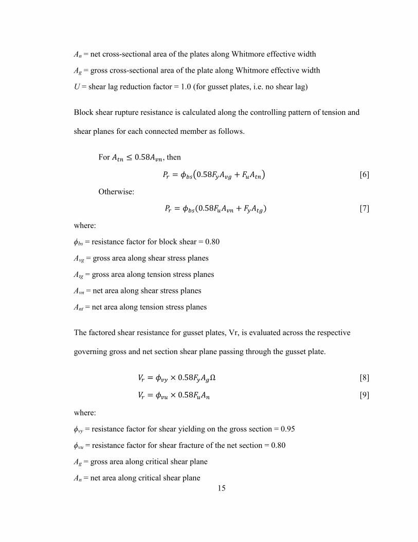
Block shear rupture resistance is calculated along the controlling pattern of tension and
shear planes for each connected member as follows.
For , then
[6]
Otherwise:
[7]
where:
ϕbs = resistance factor for block shear = 0.80
Avg = gross area along shear stress planes
Atg = gross area along tension stress planes
Avn = net area along shear stress planes
Ant = net area along tension stress planes
The factored shear resistance for gusset plates, Vr, is evaluated across the respective
governing gross and net section shear plane passing through the gusset plate.
[8]
[9]
where:
ϕvy = resistance factor for shear yielding on the gross section = 0.95
ϕvu = resistance factor for shear fracture of the net section = 0.80
Ag = gross area along critical shear plane
An = net area along critical shear plane
Page 27
16
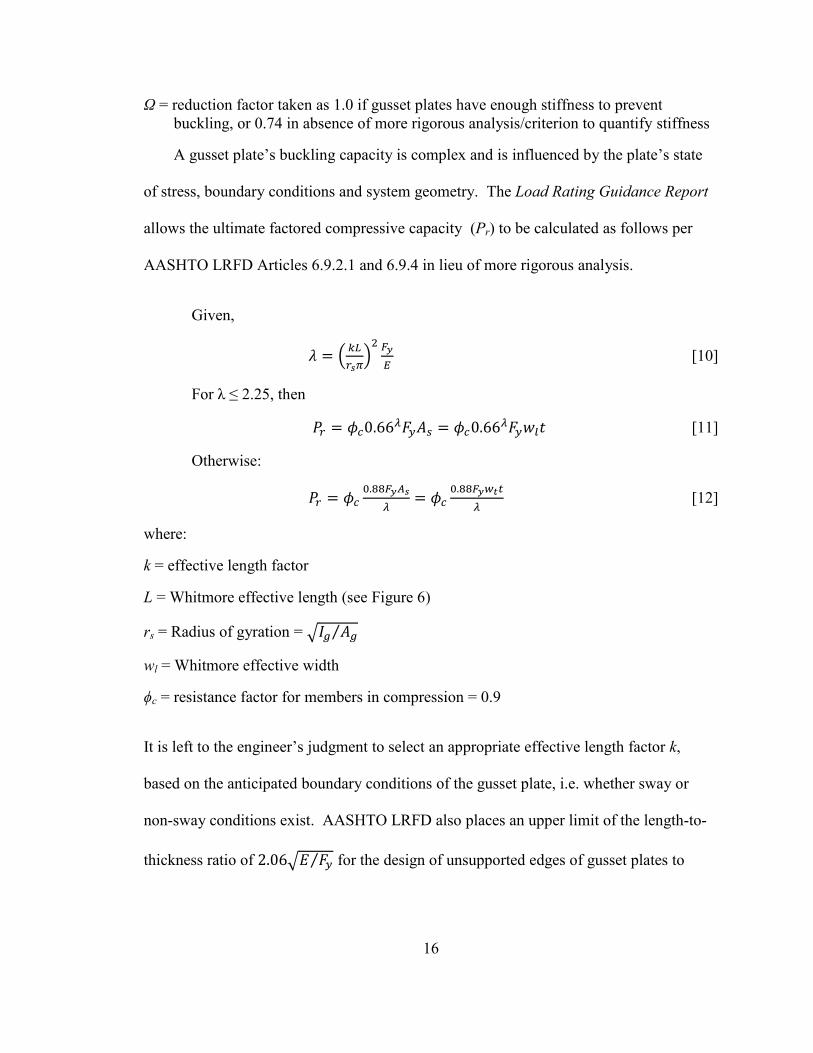
Ω = reduction factor taken as 1.0 if gusset plates have enough stiffness to prevent
buckling, or 0.74 in absence of more rigorous analysis/criterion to quantify stiffness
A gusset plate’s buckling capacity is complex and is influenced by the plate’s state
of stress, boundary conditions and system geometry. The Load Rating Guidance Report
allows the ultimate factored compressive capacity (Pr) to be calculated as follows per
AASHTO LRFD Articles 6.9.2.1 and 6.9.4 in lieu of more rigorous analysis.
Given,
[10]
For λ ≤ 2.25, then
[11]
Otherwise:
[12]
where:
k = effective length factor
L = Whitmore effective length (see Figure 6)
rs = Radius of gyration =
wl = Whitmore effective width
ϕc = resistance factor for members in compression = 0.9
It is left to the engineer’s judgment to select an appropriate effective length factor k,
based on the anticipated boundary conditions of the gusset plate, i.e. whether sway or
non-sway conditions exist. AASHTO LRFD also places an upper limit of the length-to-
thickness ratio of for the design of unsupported edges of gusset plates to
Page 28
17
prevent gusset plate buckling, but is not required by the Load Rating Guidance Report
when evaluating existing connections.
2.6 Previous FEA Gusset Plate Models
Many of the aforementioned studies developed analytical models based on the
finite element method in conjunction with their experimental work. The following is a
summary of previous methods used in the literature to model gusset plate stress
distributions and failures.
Davis (1967) was among the early users of FEA to investigate gusset plate
stresses in the elastic range, where he replicated Whitmore’s findings analytically in his
thesis research. Vasarhelyi (1971) also employed finite element analysis on stress
distributions across critical planes of the gusset plates he tested experimentally. He
reported close agreement between the analytical and experimental results, but did not
provide specific details to the analytical approach.
More recent FEA models have been developed using Abaqus finite element
software to model tensile and compressive failure states. Walbridge et al. (2005)
presented a model to investigate gusset plate failure states under monotonic tension,
compression and cyclic loading. The model was based upon previous analytical models
developed by Yam and Cheng (1993), which were used to model gusset plate buckling
capacity. Abaqus S4R shell elements were used to model the gusset plate. Both a perfect
elasto-plastic and isotropic strain-hardening material models were examined. Load was
delivered through two splicing members on each side of the gusset plate; with the bolt
connections modeled as either rigid beam elements, or as one-dimensional spring
elements to incorporate load displacement behavior of the fasteners. Bolt holes were not
Page 29
18
explicitly modeled in the gusset plate. The model was calibrated with experimental data
from Rabinovitch and Cheng (1993) and Yam and Cheng (1993).
Walbridge found that the perfect elasto-plastic material model produced better
predictions of ultimate tensile strength, whereas the isotropic strain-hardening model
tended to over-predict ultimate tensile strength. Walbridge hypothesized this may be due
to the exclusion of bolt holes in the model, and that the excess material along the block
shear failure planes contributed to the model’s overstrength. Buckling capacity was
significantly affected by the magnitude of initial out-of-plane distortion introduced in the
gusset plate prior to loading, as well as the state of boundary conditions imposed on the
splicing members. It was also found that incorporating load-displacement behavior of the
fasteners had little effect on the predicted global load-displacement behavior of the plate,
or the predicted ultimate strength in tension and compression.
Sheng et al. (2002) used a model analogous to Walbridge’s model to conduct a
parametric study on gusset plate buckling strength. Among the parameters considered
included the effects of unsupported edge length, degree of rotational restraint imposed on
the brace member, and the stiffness and length of the brace member. It was shown that
increased unsupported edge length, increased rotational restraint, decreased brace
member flexural stiffness and increased brace member length, all decreased the gusset
plate’s buckling capacity.
Following the I-35W Bridge collapse in Minneapolis, a detailed finite element
model was constructed to elucidate on the hypothesis that collapse was initiated at an
under-designed gusset plate, and is described by Liao et al. (2011). A global model of
the entire bridge was developed using the software SAP 2000 to determine the load
Page 30
19
demands on the U10 connection through the bridge’s service life. A connection-level
model of the U10 connection was developed using Abaqus. The gusset plate was
modeled using C3D8 (linear brick element) elements from the Abaqus element library.
Member stubs were included in the connection model. Rivets and their corresponding
holes were explicitly modeled at the L9/U10 diagonal, represented by rigid cylindrical
shells that transferred load through contact interaction to the rivet holes in the gusset
plate. Rivets on the remaining sections were modeled with rigid beam elements through
the hole centers. The contact interaction definition between the rivets and bolt holes
neglected tangential friction. The model represents the highest degree of complexity in a
gusset plate connection reported in the literature, containing approximately 120,000
elements per gusset and was run on an IBM Power4 supercomputer at the University of
Minnesota Supercomputing Institute.
Conclusions from the FEA study corroborated the forensic and design review
investigations by the NTSB (2008), namely that a significant portion of the U10 gusset
plates may have already been yielded at the time of collapse. The added construction
weight, combined with insufficient strength at the U10 node were the main contributors
to the bridge’s collapse. Liao also suggested that the interaction between compression
and shear may have played an important role in the failure and recommended further
study.
2.7 Summary
The conclusion that gusset plate tensile capacity is governed by block shear is
well established in the literature. Although equations for calculating block shear differ
slightly between Hardish and Bjorhovde (1985), AISC Specifications, and AASHTO,
Page 31
20
they all are capable of adequately predicting gusset plate tensile resistance with varying
levels of conservatism. On the other hand, compressive capacity is considerably more
challenging for a designer to assess given the current design approach, which relies on
reducing the gusset to some equivalent column and selecting an appropriate effective
length factor. This problem manifests itself in the literature by numerous alterations
presented – such as adjusting the Whitmore block definition, or using different effective
length factors – in order to align calculated buckling capacity with experimental and
analytical results. Also, the magnitude of out-of-plane gusset plate are not incorporated
into design or load rating procedures per the Load Rating Guidance Report, which can
have a significant impact on buckling capacity.
Page 32
21
3.0 Numerical Modeling
3.1 Objectives
The primary goal of this effort is to develop a calibrated FEA model capable of
evaluating gusset plate stresses and ultimate strength limit states. Experimental data from
ongoing research at Oregon State was provided to validate the connection model. A
secondary objective was to develop a gusset connection model such that it could be
readily adapted to analyze multiple connection geometries while minimizing the
development process. This was realized by utilizing the Abaqus scripting environment to
automate a significant portion of the model development, thereby aiding in existing
parametric studies and building in the capability for rapid analysis across multiple
connection in future studies. Representative scripts used to construct some of the small-
scale bolt models and gusset plate connection models are included in Appendix B.
Finally, computational efficiency was addressed by examining a number of modeling
techniques, ranging from simplified to more robust; to assess the level of detail required
to obtain accurate results.
3.2 Fastener Modeling
Several approaches exist for modeling bolts and their load transfer through shear
from one plate to another. The method chosen to model bolted connections has the
greatest influence on the overall complexity of the connection model, particularly when
considering the large number of fasteners found in bridge connections. Typically, two
approaches are taken; modeling the bolted connection with or without the bolt holes
included in the plate. Exclusion of bolt holes is the simplest approach from a
Page 33
22
development point of view, though may not be able to capture net section-related failure
modes. Conversely, inclusion of the bolt holes may better capture plate behavior, since
bolt holes can account for a significant amount of material lost along net-section fracture
planes, but adds significant complexity to the model by creating complicated meshing
tasks, increased number of elements and difficulty in applying realistic loads to the inner
hole surfaces. The application of load to the bearing surfaces of the bolt holes also poses
significant challenges for the modeler. One approach to alleviate this is to define
equivalent edge loads along the anticipated bolt hole contact surface. This method has
been used successfully by Huns et al. (2006) to model block shear failure modes and
yielded analytical results close to experimental values. However, this approach is only
valid when the direction of load application is known, and equal distribution of load
between all fasteners in the member connection is assumed; neither of which may be
appropriate for bridge connections.
3.2.1 Beam Element Bolt Models
Perhaps the simplest and most common method is to idealize bolts as a one-
dimensional rigid beam element that ties all degrees of freedom between the two
connected nodes, where the nodes correspond to the bolt hole centers on adjoining plates.
In Abaqus, this is achieved by using a rigid multi-point constraint (MPC) element
positioned at the bolt hole center between two connected plates. Note that although this
study uses rigid definitions for its beam element bolt models, Abaqus does allow
experimental load-displacement behavior and failure criteria to be incorporated into the
MPC element definition. Several examples exist in the literature that use this method,
Page 34
23
with and without fastener load-displacement behavior, to represent bolted connections
(Walbridge et al. (2005), Sheng (2002), Ocel and Wright (2008)).
A related bolt modeling approach is the use of Abaqus Fastener (AF) elements, a
proprietary element formulation similar to MPC elements, except that a radius of
influence equal to the bolt radius about each connection point is added to the element
definition. All elements inside the radius of influence are rigidly tied to the connection
points, thereby “including” the influence of the bolt without explicitly modeling the bolt
hole itself.
3.2.2 Three-Dimensional Contact Bolt Models
Three-dimensional (3D) contact modeling of bolt-plate interaction represents the
most detailed method for modeling load transfer of a bolt through bearing on to a plate,
and is correspondingly the most demanding regarding model development and
computation time. This approach requires the use of a three-dimensional solid
representation of the gusset plate, since shell element formulations lack numeric stability
when contact is imposed along the shell edge. Several examples of 3D contact bolt
models exist in the literature, most of which are limited to simple connections with only a
few bolts. Chung and Ip (2000) developed a 3D contact model to investigate failure of
bolted lap connections under tension. Correlation between experimental and analytical
results were good, however several simplification measures were taken – including the
use of symmetry, rigid definitions of the bolt, out-of-plane restrains, and the number of
bolts (3 maximum) – in order to obtain workable computation times. Ju et al. (2004)
expanded on Chung and Ip’s model by including elasto-plastic behavior in the bolt
shanks, bolt pre-tension and steel material failure criteria. Results were compared per
Page 35
24
AISC Specifications, which were in good agreement with analytical results. However,
the connections considered were single lap joints with a maximum of three bolts subject
to monotonic tension.
The largest scale known by this author of the use of 3D contact bolt modeling in a
structural engineering application is in the FEA model presented by Liao et al. (2011),
which was developed to investigate the U10 gusset failure on the I35-W Bridge in
Minneapolis. The model used 3D contact interactions to model load transfer from rivets
(152 in total) at the L9-U10 compression diagonal to the gussets, with the bolts being
idealized as rigid cylindrical shells. The remaining rivets in the connection were modeled
with rigid MPC elements. The model delivered a high level of detail regarding the
locations and progressions of yield zones in the gussets, but at significant computational
cost as illustrated by the investigators’ decision to limit the implementation of the 3D
contact bolts to the L9-U10 diagonal, and the use of the University of Minnesota
Supercomputing Institute to run the model.
3.2.3 Radial-Spring (RS) Bolt Model
In an effort to develop a shell-compatible bolt model analogous to 3D contact bolt
models discuss above, a simplified idealization of a bolt was constructed out of one-
dimensional elements. Named the Radial-Spring (RS) bolt model and shown Figure 12,
this simplified model consists of three distinct types of one-dimensional elements. A
rigid MPC beam element is oriented along the bolt shank connecting the member to the
gusset plate. Non-linear spring elements with high compressive stiffness and very low
tensile stiffness transfer bearing loads from the MPC beam element to the gusset plate
bolt hole. Four wire elements radiating from the member-side of the MPC beam element
Page 36
25
to the bolt hole edges define a slip-plane restraint. The slip-plane restraint elements
added necessary stability to the radial spring array by allowing free translation of the bolt
hole edges within the plane of the gusset plate, but preventing the hole from moving out-
of-plane relative to the member. In essence, the slip-plane restraint simulates clamping
between the bolt head and outer plate preventing excessive deflections of the hole along
the bolt shank axis under high loads. Preliminary investigations showed that using four
slip-plane restraint elements was the minimum required to stabilize the radial spring
element array. The RS bolt model is similar in formulation to one proposed by Siekierski
(2009), who compared several simplified bolt modeling techniques in angle-gusset
connections subject to tension, one of which used a radial array of non-linear spring
elements to transfer bolt bearing loads to the plate. Siekierski’s bolt model differed in
that it included radial spring arrays on both sides of the bolt and lacked a slip plane
definition. Siekierski incorporated a second array of beam elements placed at the plane
of contact between the bolt head/nut and the outer steel plate surface to simulate the
clamping force from the bolt head and nut.
3.3 Single Bolt Connection Model
An Abaqus model was created to compare the above-mentioned fastener
modeling techniques. A single bolt model was used to select appropriate shell elements,
establish a rational mesh regime and compare load-displacement behaviors. Parallel
experimental tests were not conducted for this phase, because there is sufficient data in
the literature showing 3D contact bolt modeling correlates closely with experimental data
for simple connections in tension. Therefore, a 3D contact bolt model – using modeling
Page 37
26
strategies consistent with published studies – was used as the benchmark to compare
against the MPC, AF and RS bolt models.
For the 3D contact model, a 6-3/8” x 3-3/4” x 1/4" plate with a fixed base and a
3/4” diameter bolt hole positioned at the top was used (see Figure 13a). The fixed base
boundary condition was considered realistic for modeling a simple plate subject to
tension. The minimum edge distance from the bolt hole to plate edge was 1-1/2”. The
bolt shank was idealized as a rigid cylindrical shell positioned at the hole center. C3D8
elements from the Abaqus element library were used throughout the plate, with three
layers of elements distributed across the plate thickness. A partition consisting of a circle
twice the hole diameter and a centered horizontal and vertical lines was created around
the bolt hole to establish uniform element distribution. A structured mesh and advancing
front algorithm were used to mesh the bolt hole partition and remaining plate
respectively. The mesh refinement around the bolt hole was set to match the final mesh
used in the RS bolt model. Global seed values were used on the remaining plate mesh to
create element sizes close to those found in the bolt hole partition. Material properties
were assigned as described in Section 3.4. A “hard” contact interaction was defined for
normal behavior and tangential behavior was defined as “smooth sliding”; in other words,
surface friction on the bolt hole surface was neglected. This was justified since it is not
possible to replicate tangential friction in the current RS bolt model formulation, even
though friction forces do exist in actual bolt hole-bearing interactions. Displacement was
imposed on the bolt shank to load the plate in tension.
The plate used for the RS bolt model was idealized as a shell with an identical
profile and assigned the same thickness as the 3D contact model (see Figure 13b). The
Page 38
27
bolt shank was idealized as a rigid beam element positioned at the hole center. S4 and S3
elements were selected from the Abaqus element library for the shell portions of the
model. The radial spring array consists of axial spring elements radiating from the hole
center to equally spaced vertices around the bolt hole. Non-linear stiffness definitions
were assigned to the radial springs with very low tensile stiffness (0.01 kip/in) and high
compressive stiffness (711.5 kip/in for 32 radial springs on 1/4” plate). Compressive
stiffness was calculated based on an equivalent wedge-shape section of a shank from an
A325 bolt and having the same thickness as the plate. Preliminary studies showed that
load-displacement behavior was not sensitive to varying compressive spring stiffnesses.
Vertical displacement was imposed at the hole center to simulate tensile loading of the
plate.
The MPC beam and AF bolt models used the same plate dimensions, shell
formulations and boundary conditions as the RS bolt model, except that no hole was
included in the plate. The AF element was assigned a radius of influence of 3/8” which
corresponds to the 3/4" bolt hole A “structural distribution” rule was used to define the
constraint method for elements falling within the radius of influence. A structured mesh
algorithm was used to obtain a plate mesh refinement equivalent to the RS bolt model.
An additional base plate was included with the test model in the assembly in order to
provide two surfaces of which to attach the MPC and AF elements. The base plate was
given a fixed boundary condition and displacement was imposed on the bottom of the test
plate to achieve tensile loading.
Page 39
28
3.3.1 Single Bolt Connection Model - Results and Discussion
Convergence trials were conducted on the RS bolt model to establish the
minimum number of radial springs required, and the degree of local mesh refinement
required. Global load-displacement behavior under tension was chosen as the
convergence metric. Figure 14 shows load-displacement behavior as a function of the
number of radial springs used, where it was determined that 32 equally spaced radial
springs were required for convergence. Next, load-displacement behavior was checked
for convergence for four local meshes of increasing refinement (Figure 15), where it was
determined that two element layers around the bolt hole were sufficient.
The distribution of equivalent plastic strain (PEEQ) and load-displacement
behavior are shown in Figure 16 and Figure 17 respectively for the single bolt models.
The RS bolt and 3D contact models were in very close agreement regarding load-
displacement behavior and the location of plastic deformation. The MPC beam model
generated significantly different behavior compared to the 3D contact model; although
this can be expected due to the lack of a bolt hole in the plate, and the fact that the MPC
beam is delivering what is essentially a point load, inducing highly localized effects. The
AF bolt model produced a load-displacement curve with a similar shape to the 3D contact
model, however with significant overstrength. This can be explained by examining the
PEEQ contours and deformed shape of the plate, where necking of the plate occurs below
the connection point. The rigid radius of influence used in the AF definition engages all
of the material surrounding the hole, forcing the zone of plastic deformation on the
tension side of the bolt hole and thus increasing its tensile capacity. In essence, the AF
Page 40
29
behaves more like a spot weld than a bolt acting in bearing, and indicates that the using
this technique to model bolt bearing-plate interactions should be done judiciously.
3.4 Multi-Bolt Connection Model
In order to test the bolt models’ performance in capturing gusset plate tensile
failures on a small scale, a series of experiments were conducted on small-scale gusset
plates. The two samples, denoted Sample A and B, were designed to fail in net-section
rupture and block shear respectively (Figure 18). Both samples were made from 3/16”
thick A36 mild steel plate and tested on a MTS vertical load frame equipped with a 110
kip capacity actuator. The upper and lower grips were constructed to connect the
samples to the load frame and were designed to remain elastic under test loads. Load was
measured from an in-line load cell. Plate displacement was measured with a linear
displacement transducer (LDT) as pictured in Figure 19.
The approaches used in the single bolt models were applied to create the multi-
bolt connection models. A few additional partitions were added to the plate in order to
smooth the mesh transition from the bolt holes to the plate. All four previously modeling
methods were compared to experimental results. Steel coupons were prepared from the
same material used to make the test samples, in both longitudinal and transverse
directions relative to the rolling orientation. True stress-strain data was then calculated
from an average of the longitudinal and transverse coupon data, and an approximate
relationship was input into the Abaqus plasticity definition (Figure 20).
Page 41
30
3.4.1 Sample A - Results and Discussion
The observed experimental failure mode for Sample A was net-section rupture
along the bottom row of bolts at the weak connection. Experimental and analytical
capacities for Sample A are compared with the nominal block shear tensile capacities per
the Load Rating Guidance Report in Table 1Error! Reference source not found..
Analytical to experimental (A/E) ratios are to show analytical deviations from the
experimental values; where values less than one indicate a conservative prediction and
values greater than one indicate a non-conservative prediction. Figure 21 and Figure 22
show PEEQ contours and load-displacement behaviors from the four models and
experimental results from Samples A. Material damage definitions were not included in
the models material definitions, in order to maintain high computational efficiency.
Therefore “failure” of the analytical sample was defined as the greater of the maximum
load reached, or the load corresponding to a vertical displacement at which the
experimental sample reached maximum tensile strength. For Sample A, the displacement
associated with maximum experimental tensile strength was 0.2”.
The calculated net-section rupture capacity of Sample A per the Load Rating
Guidance Report gave a conservative estimate of strength with an A/E ratio of 0.92.
Both the 3D contact and RS bolt models gave conservative predictions of capacity as
indicated by the A/E ratios of 0.90 and 0.89 respectively, as well as similar load-
displacement behavior. Sample A results showed that both the 3D contact and RS bolt
models developed PEEQ contours consistent with rupture along the bottom row of bolts
on the weak connection, similar to the observed failure mode in the experimental sample.
The MPC and AF element models showed overstrength compared to the experimental
Page 42
31
results, with A/E ratios of 1.4 and 1.1 respectively. The reason for this can be seen in the
PEEQ contours, which indicate the majority of plastic yielding occurring in the gross
section below the weak bolt group for the MPC and AF element models. The MPC and
AF models reflect this since the gross section has greater capacity than the net section.
The lack of holes made it difficult for the MPC and AF models to closely capture net-
section effects in Sample A.
3.4.2 Sample B - Results and Discussion
The observed failure mode for Sample B was block shear at the weak connection.
Experimental and analytical capacities for Sample B are summarized and compared in
Table 1Error! Reference source not found.. Ultimate tensile capacity for the analytical
models was defined as the greater of the maximum load reached, or the load
corresponding to a vertical displacement at which the experimental sample reached
maximum tensile strength. For Sample B, the maximum tensile capacity occurred at a
displacement of 0.3”.
Figure 23 and Figure 24 show PEEQ contours and load-displacement behaviors
from the four models and experimental results from Samples B. The calculated block
shear capacity for Sample B per the Load Rating Guidance Report gave a conservative
estimate of strength with an A/E ratio of 0.91. Both the 3D contact and RS bolt models
also gave conservative predictions of capacity as indicated by the A/E ratios of 0.87 and
0.94 respectively, as well as similar load-displacement behavior. However, the 3D
contact model failed to reach a solution before the model failure criteria was met and may
have an artificially low tensile capacity as a result. The 3D contact and RS bolt models
Page 43
32
developed PEEQ contours consistent with block shear failure along the shear and tensile
rupture planes at the weak connection, similar to the observed experimental failure mode.
The MPC and AF element models showed significant overstrength compared to the
experimental results, with A/E ratios of 1.37 and 1.64 respectively. Unlike the net-
section rupture models, yielding developed over the shear block planes on all four
models. However, the exclusion of holes in the MPC and AF models significantly
increases the material along the shear and tension planes and correspondingly artificially
increased their tensile capacity predictions.
3.4.3 Summary
On a small scale, different bolt modeling methods have a considerable impact on
predicting tensile failure. The MPC and AF models failed to reproduce net-section failure
consistent with the experimental results, and exhibited overstrength when compared to
analytical predictions. The 3D contact and RS bolt models were able to both predict
ultimate failure and generate PEEQ profiles consistent with the observed experimental
failure state. Further, the 3D contact and RS bolt models tracked well with experimental
load-displacement curves and each other. This suggests that the RS bolt modeling
approach, when properly formulated, can act as a 3D contact modeling equivalent in
shell-formulated plates.
3.5 Gusset Connection Model Description
The connection-level gusset plate model was developed using Abaqus 6.9. The
three primary metrics were chosen to evaluate the gusset connection were elastic stresses,
and gusset plate capacity at M4 under tension and compression. Only one connection
Page 44
33
geometry was considered in this study, analogous to the specimen tested being used in a
parallel experimental study at Oregon State University. The experimental test setup and
FEA model are shown in Figure 25(a) and (b). The connection consists of a bottom
chord (M1 and M5), a vertical chord (M3), and two diagonal chords (M2 and M4). M1
and M2 are fixed on the experimental load frame and actuators are attached to M3, M4
and M5, each capable of delivering compressive loads. Global boundary conditions were
imposed at the ends of each member such that they reflected the conditions found in the
experimental tests. Members were modeled with a combination of wire and extruded
shell features; with the transition occurring where the members overlapped the gusset
plates (Figure 26). The beam-to-shell junction in each member was rigidly tied to form a
continuous member. Partitions were created on the shell portion of the member to define
vertices corresponding to bolt hole centers. The actuator load capacities, along with the
boundary conditions are illustrated in Figure 27. The gusset plate was designed to fail in
compression at M4 by reducing the bolt spacing at the M4-gusset connection, which
effectively narrowed the Whitmore effective width and increased the Whitmore effective
length. This was to help develop a rational instrumentation plan by knowing the failure
zone prior to testing, as well as insure the connection’s strength capacity was kept within
the testing limits of the actuators.
Three different gusset connection models utilizing the three bolt models described
in Section 3.3 were implemented, hereinafter referred to as the MPC, AF and RS bolt
models. Python scripts were concurrently developed to automate the construction and
assembly of the gusset connection model. The MPC and AF bolt models were the least
complex, using a single wire element to represent each bolt. The RS bolt model was
Page 45
34
substantially more complex. For each RS bolt, a hole must be created in the gusset,
partitioned, individually meshed, and connected to the plate with 38 individual wire
elements (32 radial spring, 1 MPC element, 4 slip-plane elements); meaning that for our
gusset connection with 608 bolts, there are 23,104 wire elements required just to model
the bolts. Additionally, the gusset plate mesh must be significantly denser to
accommodate the required local element density around each hole. Based on the single
bolt connection modeling, each hole requires a local mesh containing 64 elements.
Combined with the transition from the local bolt meshes to the plate mesh, this translated
to a roughly 10 fold increase in the number of gusset plate elements compared to the
MPC and AF elements. The only way to fully implement RS bolts on a connection with
so many bolts in a timely manner is by using Python scripts, which can automate this
process. A Python script used to construct the RS bolt gusset connection model through
the assembly and meshing process is included in Appendix B. Subsequent model
development tasks, such as loading, steps, boundary conditions and output were carried
out in the graphic user interface in Abaqus.
3.5.1 Material Modeling
An isotropic hardening material model was used for the gusset plates, which
requires true stress-strain data derived from coupon tests. This data was not available at
the time of this writing, so coupon data from the multi-bolt connection tests described in
Section 3.4 were substituted. Inspection of the gusset plate mill certs from Tests 1 and 2
reported Fy and Fu values within 10% of the coupon data. Material for the members was
Page 46
35
modeled as perfectly elastic, with a Young’s modulus of 29,000 ksi. This was justified
since the members from the experimental specimens were designed to remain elastic
under all foreseen loading conditions. Modeling the members as perfectly elastic
increased computational efficiency and insure that failure always occurred in the gusset
plate.
3.5.2 Element Selection
Gusset plates were modeled as shells in order to avoid the additional development
time and computational requirements associated with 3-dimensional modeling. S4 and
S3 elements were selected from the Abaqus element library for the shell portions of the
model. The S4 shell element is a rectangular element and the S3 element is a triangular
element; both are fully integrated, finite-membrane-strain shell elements suitable for
large-strain analysis (Simulia, 2010). The B31 element was selected for the beam
portions of the model; which uses a Timoshenko beam formulation with a linear
interpolation function and is suitable for both stout and slender beams (Simulia, 2010).
3.5.3 Mesh Refinement
A stress convergence trial was conducted to determine the gusset plate mesh
necessary to converge on stresses under elastic loads. MPC element modeling was
selected to represent bolts in the connections, due to their ease of implementation. Mises
stress, sxx, syy and sxy were monitored at nodes spaced along Planes A and B, with each
node corresponding to positions of strain gages from experimental tests (see Figure 28).
The subscripts refer to stress in the global x, global y and shear stress in the xy plane
respectively. Convergence was defined as the point where stress change due to increased
Page 47
36
number elements was less than 5%. Convergence plots for Mises, sxx, syy, and sxy stresses
from sample points on Planes A and B are available in Appendix C. Both Mises and sxy
stresses converged rapidly and satisfied the convergence criteria at 2892 elements and
6082 elements, respectively. Convergence was more problematic at sampling points A3
and B2 for sxx, and sampling point A3 for syy due to their locations in a high stress zones
on the gusset plate. However, the majority of sampling points converged readily. It was
ultimately determined that a mesh of approximately 6500 elements per gusset plate was
sufficient for monitoring stresses at the most of sampling points in the elastic range.
Identical gusset plate meshes were used for MPC and AF bolt models. For
models using RS bolts, local meshing strategies used in the single-bolt connection model
was deployed to every bolt hole in the gusset plate. The advancing front meshing
algorithm initially produced a prohibitively large number of elements on the gusset plate.
This was resolved by drawing additional partitions on the gusset plate. A global seed
definition was defined to regions outside of the local bolt meshes to create a mesh of
comparable density to that used for the MPC and AF models. Gusset plate partitions and
meshes for RS and MPC/AF models are compared in Figure 29.
3.5.3 Elastic Stress Analysis
Gusset plate stresses due to member loading were analyzed with the specific goals
of mapping gusset plate stress contours and identifying changes in the stress profile due
to different loading patterns. MPC, AF and RS bolt models were compared. Loading of
the gusset plate was delivered by members M3, M4 and M5 such that gusset plate
stresses were kept in the elastic range. No initial out-of-plane distortions introduced into
Page 48
37
the model for the elastic stress analysis. The Static-General step module was used to run
the analysis.
Three load sets were selected for analysis and are shown in Table 2. Global
trends were tracked qualitatively using stress contours in order to compare the different
bolt modeling techniques, and quantitatively across critical stress planes to make
comparisons between analytical and experimental values, as shown in Figure 28. Plane
A lies directly above and parallel to the horizontal chords, and is a critical plane used to
check the gusset for gross section yielding and one identified by Whitmore as the location
of maximum shear stress. Plane B lies directly behind the last bolt row on the M4
diagonal and corresponds to the location of maximum normal stresses as described by
Whitmore.
3.5.4 Buckling Capacity Analysis
Three Abaqus analysis methods were considered for evaluating the buckling
capacity of the gusset plate at the M4 diagonal: eigenvalue buckling analysis, the Static-
Riks and Explicit-Dynamic step modules. Buckling at M4 was only considered in order
to stay relevant to the experimental test conducted at Oregon State (see Section 3.7).
Eigenvalue buckling analysis is the simplest, where the bifurcation load and buckling
shape are estimated by solving the classic eigenvalue problem for system buckling. The
first mode is typically the one of interest in static loading problems, since its associated
eigenvalue is a rough estimate of the bifurcation load, and its mode shape represents the
manner which the system will buckle. It cannot take into account non-linear material
behavior such as plasticity, which is why eigenvalue buckling analysis by itself is not
Page 49
38
recommended for systems where nonlinearity is anticipated (Simulia, 2010). For this
study, the first mode buckling shape was used to introduce various degrees of out-of-
plane imperfections into subsequent modeling steps in order to induce buckling in the
nonlinear models.
The Static-Riks module in Abaqus uses an implicit-based direct stiffness approach
and is capable of analyzing systems with high geometric and material non-linearity,
coupled with a modified Riks algorithm to track the load-displacement path of the system
through successive increments (Simulia, 2010) . The modified Riks method works well
for analyzing unstable systems such as buckling where load and/or displacement may
decrease as the solution progresses, and is a valid approach assuming loading is smooth
and can be scaled with a single parameter (Simulia, 2010).
The Explicit-Dynamic step module is capable of analyzing complex systems with
high geometric non-linearities and contact definitions, making it another candidate to use
in buckling analysis. Although originally developed to analyze highly dynamic systems,
the method can be used for pseudo-static loading, provided care is taken to insure the
applied load rate does not impart excessive inertial effects into the system. The Explicit-
Dynamic module uses an explicit integration rule combined with a lumped element mass
matrix to kinematically advance the solution from one increment to the next. This makes
the solution of each increment highly efficient, as it does not require the assembly of a
system mass matrix and the solution of a large number of simultaneous equations. The
size of a stable increment is considerably smaller compared to implicit methods, but is
counterbalanced by the ability to execute each increment much more rapidly. In cases of
Page 50
39
high model complexity, the Dynamic-Explicit module is a viable way to investigate
buckling behavior.
Load was induced in the connection by applying a vertical displacement of 0.5” in
the global y direction until failure. This was to simulate the testing conditions used at
Oregon State. Preliminary tests showed that the axial load and global behavior of the
model were extremely close to when the displacement was applied axially down the
member. MPC, AF and RS bolt models were used to model the bolted connections. The
linear buckling load was determined by solving for the first mode eigenvalue for the
entire connection model subject to a unit axial compressive load along the M4 diagonal.
In order to initiate buckling in the non-linear model, a out-of-plane distortion equal to the
first buckling mode scaled to 25% the plate thickness at the free edge was introduced
prior to loading. For a 1/4" thick gusset, this means that the initial out-plane distortion at
the gusset plate free edge was equal to 1/16”. For the Static-Riks method, a displacement
criterion of 2 inches out-of-plane displacement at the gusset vertical free edge was used
to halt the analysis. A load rate convergence trial for the Explicit-Dynamic step module
was conducted to insure that inertial forces were low and the static response remained
dominant.
The effect of gusset plate mesh refinement on global behavior was also checked
for convergence by looking at the elastic buckling load from an eigenvalue buckling
analysis and load-displacement behavior. The Static-Riks solver was used to arrive at a
solution for the non-linear model. Refer to Appendix C for global behavior convergence
Page 51
40
plots. It was determined by inspection that a mesh of approximately 6000 elements was
adequate for capturing global connection behavior.
3.5.5 Tensile Capacity Analysis
No tensile capacity tests were included in the Oregon State experimental testing
program, so analytical values of M4 tensile capacity was compared to the nominal block
shear design strength per the Load Rating Guidance Report. MPC, AF and RS bolt
models were considered, and the Static-General solver was used. Preliminary
investigations showed the Static-General and Static-Riks solvers produce equivalent
results for tensile failures. No initial modal imperfections were introduced in the models
subject to tension. Tensile load was induced in the connection by applying a vertical
displacement of 1.5” along in the M4 axial direction until failure.
3.6 Gusset Connection Experimental Program (Oregon State)
Three experimental tests were conducted at Oregon State and provided the data to
validate the FEA model and are summarized below.
3.6.1 Test 1 – Description and Results
Test 1 used 1/4” gusset plates, and was tested under several loading combinations in
increasing magnitude until failure. The loading protocol for Test 1 consisted of a series
of sets, grouped by the load magnitude at M4 (Table 3). Strain gage data on the gusset
plate was collected at each set. Axial load of the members was determined by an array of
strain gages attached between the member connection and member end. The magnitude
of the load sets increased incrementally until failure. Initial out-of-plane imperfection
was assessed by Electronic Speckle Laser Interferometry (ESLI), and determined to be
Page 52
41
approximately 25% of the plate thickness. See Figure 34 for a comparison between out-
of-plane displacement contours from ESLI and the first buckling mode shape from
eigenvalue buckling analysis.
The mode of failure was in buckling at the M4 diagonal which occurred at a
bifurcation load of 270 kip. An effective length factor of k = 0.61 was found by back-
calculating from the experimental buckling load according to the Load Rating and
Guidance Report. Figure 35 compares the post-buckled shape from Test 1 and FEA
model. Contours on the FEA model indicate out-of-plane displacement, and M4 has been
removed for clarity. The timing at which buckling occurred in Test 1 was somewhat
unexpected, being that the gusset buckled while the M4 diagonal was loaded at
approximately 275 kip and the M5 was in the process of being unloaded from 225 kip to
zero.
Due to the many load combinations tested and a low low-frequency sampling rate,
load-displacement behavior was not captured in Test 1 at the time of buckling. However,
the strain gage data obtained was used to compare with analytical values in the elastic
range. Three load sets (100 kip, 175 kip, 250 kip) from the Test 1 data were selected to
make stress comparisons between experimental and analytical values. Comparisons were
made in two ways. The first, used the 100 kip load set to examine the effects of loading
combinations of the horizontal chord (M5), vertical chord (M3) and diagonal chord (M4)
have on the stress profiles across Planes A and B. The second comparison was made
between M4 loaded at 100 kip, 175 kip and 250 kip, while M3 and M5 were kept at 1 kip,
to estimate the resulting Mises stress increases across Planes A and B. Stresses were
calculated from strain assuming elastic conditions with E = 29,000 ksi, then transformed
Page 53
42
into a global xy orientation. Positive values indicate tensile stresses and negative values
indicate compressive stresses. Stress in the global x (sxx), global y (syy), shear stress in
the xy plane (sxy) and Mises stresses were examined positioned at sampling points along
Planes A and B (see Figure 28).
Results for the experimental stress profiles along Plane A are presented in Figure
36 through Figure 39. The x-axis in these figures plots stresses from the left gusset edge
to the right along Plane A due to load combinations from M4 only, M4 + M5, and M3 +
M4 + M5, with load magnitudes of 100 kip for M4, 94 kip for M5, and 24 kip for M3.
Maximum Mises, sxx and sxy stresses occurred at the strain gage 38” from the left edge of
the gusset; the zone corresponding to the gap between M1 and M5. Experimental values
for syy fell within 4 ksi and 5 ksi at strain gages between 15” and 55” along Plane A.
Both Mises and sxy stresses increased on the left side of Plane A and decreases on the
right side of Plane A due to preloading from M5 and M3. The positive values for sxx
indicate the presence of tensile stresses in the x-direction, which is contrary to intuition
and to analytical results. sxx decreased significantly in response to preloading of M5, but
little due to preloading of both M5 and M3. Changes in syy showed minimal effects due
to M5 and M3 preloading.
Results for the experimental stress profiles along Plane B are presented in Figure
40 through Figure 43 . Plane B follows the Whitmore effective width along the last bolt
row from M4. The x-axis in these figures plots stresses from left to right along Plane B
due to load combinations from M4 only, M4 + M5, and M3 + M4 + M5, with load
magnitudes of 100 kip for M4, 94 kip for M5, and 24 kip for M3. Maximum Mises, syy
Page 54
43
and sxy stresses occurred at the strain gage centered in the middle of Plane B. Maximum
sxx values were again positive, indicating tensile stresses along Plane B, occurred at the
strain gages on the left and right side for the M4 only load case. sxx stress profiles for the
M4 + M5 and M3 + M4 + M5 load cases showed diminishing stresses moving from left
to right.
Figure 44 and Figure 45 shows experimental Mises stresses along Planes A and B
due to increasing M4 compression loads of 100 kip, 175 kip or 250 kip, while M3 and
M5 were each loaded to 1 kip. Mises stress profiles along Plane A increased in a linear
fashion across the entire plane due to the M4 load increases. Mises stresses along Plane
B showed in increasing trend as load increases, but not as uniformly as the Plane A stress
increases.
3.6.2 Test 2 – Description and Results
Test 2 used 1/4” gusset plates, where M4 was loaded monotonically in
compression until failure to obtain time-history data. M3 and M5 were loaded at 1 kip
each for the duration of the test. Initial out-of-plane imperfection by ESLI was
determined to be approximately 25% of the plate thickness. The mode of failure was
buckling at the M4 gusset, at a bifurcation load of 300 kip. The effective length factor k
= 0.58 was found by back-calculating from the experimental buckling load according to
the Load Rating and Guidance Report. Figure 49 shows the final buckling shape, which
is similar to the buckling shape from Test 1 except that it occurred in the opposite
direction. M4 load and out-of-plane displacement at the gusset free edge was captured
and used to compare with the analytical results, and is shown Figure 48.
Page 55
44
3.6.3 Test 3 – Description and Results
Test 3 used 3/8” gusset plates, and underwent a similar loaded protocol as Test 1
did, except that 50 kip increments on M4 were used between load sets instead of 25 kip
increments. The gussets did not fail initially using the full capacity of the actuator (550
kip), so additional out-of-plane displacement equivalent to 79% of the plate thickness
was induced using a braced hydraulic ram. The mode of failure was again buckling at the
M4 gusset, at a bifurcation load of 533 kip. Strain gage data was gathered similarly to
Test 1, but was not available at the time of this writing.
3.7 Analytical Results and Experimental Validation
Analytical results from the gusset connection elastic stress, buckling capacity and
tensile capacity analyses are summarized below, followed by a comparison with
experimental findings.
3.7.1 Elastic Stresses
A qualitative examination of the analytical stress contours from MPC, RS and AF
bolt models is presented in Figure 30 and Figure 31, showing stresses induced by a 100
kip compressive load at M4. All three models show nearly identical global stress
distributions for Mises, sxx, syy and sxy stresses. Figure 32 and Figure 33 show profile
stresses across Planes A and B for MPC, AF and RS models due to a 100 kip
compressive load at M4. All three models trended similar stress profiles, except for a
few cases. Stress deviations between the different models occurred for sxx along Plane A
at about 30” from the left free edge of the gusset; which is associated with the point
between the bottom of the M2 diagonal and M1. The other noticeable difference can be
Page 56
45
seen along Plane B, where sxx and syy values for the MPC model are lower between 12”
and 26” on Plane B; the region associated with the location of the last row of bolts on
M4. Otherwise, there were no other significant qualitative differences in plate stress
distributions from the different bolt models.
Direct comparisons between analytical and experimental stresses were made
along Planes A and B (Figure 36 through Figure 43) due to preloading at M3 and M5,
and revealed numerous differences between the analytical and experimental values. One
major distinction lies between analytical and experimental stress. Analytical stress from
the model output is in the form of membrane stresses and represents an averaged stress
across the plate thickness, whereas experimental stress is derived from strain gages that
record on the outer plate surface. Also, out-of-plane distortions can potentially color the
experimental data due to bending stresses induced in the plate. Other complications can
be associated with instrumentation and data acquisition using strain gages that may arise
in data errors. However, the author will not hypothesize or speculate as to whether this
was a factor here, since he did not directly participate in the experimental
implementation.
Striking differences can be seen with sxx on Plane A and B, and sxx on Plane B.
The positive values for sxx indicate the presence of tensile stresses in the global x-
direction, which is contrary to intuition and to analytical results considering the location
of the sampling points. The experimental profile for syy on Plane A did not track well
with the analytical either. It is less concerning that there is a difference in sign for sxy
Page 57
46
between analytical and experimental, as this may be attributed to different sign
conventions and theoretically do not affect the principal stresses.
Mises and sxy stresses (ignoring the sign difference) provided the closest
correlation between analytical and experimental values, with peak values occurring
approximately midway along Planes A and B. The trend that Mises stress increases on
the left side of Plane A and decreases on the right side of Plane A due to preloading from
M5 and M3 was also observed for analytical and experimental values. Mises stresses on
Plane B shared a common profile between analytical and experimental, although the
experimental data seemed more sensitive to change due to preloading than the analytical
data did.
The strongest correlation between the analytical and experimental can be seen in
Figure 44 and Figure 45, which plot Mises profile changes to increased compressive load
at M4 along Planes A and B respectively. An increase in load causes linear increases in
the Mises stress profiles for both the analytical and experimental along Plane A. A
similar trend occurs along Plane B, although not as close as with Plane A. This is finding
is expected since loading of gusset plate was kept within the elastic range.
In summary, more experimental data stress data is needed to fully validate the
model, although analytical values for Mises and sxy stresses were within a reasonable
margin of error. It may be helpful to increase the density of the strain gage array on the
plate in future experiments, as well as sampling strain on both sides of the plate. Another
tool in potentially validating analytical stresses is the use of ESLI to map full stress
contours across the gusset plate.
Page 58
47
3.7.2 Buckling Capacity
Load-displacement data was used to assess buckling predictions between the
different modeling approaches, where the load is the axial force in M4, and out-of-plane
displacement is measured at the midpoint of the gusset free edge between M4 and M5, as
illustrated in Figure 46. Figure 47 shows load-displacement curves for experimental Test
2 compared to MPC, AF and RS bolt models. Figure 48 similarly compares Test 2 load-
displacement curves with buckling predictions from the first mode eigenvalue, Explicit-
Dynamic and Static-Riks analysis methods using the MPC bolt model only. Table 4
summarizes the various analytical buckling capacity predictions for 1/4” gusset plates,
A/E ratios and back-calculated values for k. The experimental value used to calculate the
A/E ratios was taken as 285 kip; the average of the buckling loads from experimental
Tests 1 and 2. The post-buckling shape was the same for each model case, and is shown
along with the experimental buckled shape in Figure 35. The Static-Riks solver was
selected to assess the bolt models because it gave the closest prediction to experimental
buckling capacity, and was more computationally efficient than the Dynamic-Explicit
solver. Attempts to solve the RS Bolt model with the Explicit-Dynamic solver proved to
be computationally prohibitive. The MPC and RS bolt models gave very accurate
predictions of the experimental buckling load, with A/E ratios of 1.04 and 1.07
respectively. The AF bolt model had an A/E ratio of 1.57, significantly over predicted
experimental buckling strength. The analytical buckling capacity for the 3/8” plate 559.6
kip, assuming 75% initial imperfection, and producing an A/E ratio of 1.05.
In summary, the experimental data validates the FEA model for buckling
capacity. Use of the Static-Riks solver and the RS bolt predicted experimental buckling
Page 59
48
capacity within 4%. The use of the MPC bolt model is also a viable option for analyzing
gusset connection buckling, predicting experimental buckling capacity within 7% for the
1/4" plate and within 5% for the 3/8” plate. This makes the use of MPC bolts more
appealing for buckling analysis as it substantially cuts down on the development time
associated with the RS bolt model, while only sacrificing 3% in accuracy.
3.7.3 Tensile Capacity
No tensile capacity tests were included in the Oregon State experimental testing
program, so analytical values of M4 tensile capacity was compared to the nominal block
shear design strength per the Load Rating Guidance Report. Figure 52 shows PEEQ and
Mises stress comparisons for the MPC, AF and RS bolt models; where color contours for
Mises stresses indicate stress states beyond the yield stress in the material definition (50
ksi), and colors for the PEEQ contours indicate permanent plastic deformation greater
than 2%. Figure 51shows load-displacement curves for MPC, AF and RS bolt models.
Nominal block shear capacity was calculated to be 794 kip. A line representing the
nominal block shear capacity is included in Figure 51for reference. Table 5 summarizes
the analytical predictions and A/E ratios from each model, where the nominal block shear
design strength was used for the “experimental” values in the ratio.
The observed mode of failure was block shear at the M4 portion of the gusset,
with significant yielding and plastic deformation occurring around the outer bolt holes at
M1, M2 and M3. There were no significant deviations from the calculated block shear
capacity and the different models; the largest difference being the AF bolt model, which
over-predicted block shear capacity by 9%. The MPC bolt model over-predicted block
Page 60
49
shear capacity by 6%. The RS bolt was extremely close to the calculated block shear
capacity; so close that the A/E ratio came out to be 1.0. Examining the contours from
Figure 52 show very little plastic strain beyond 2% for the MPC model, however this
may be due to the fact that the solution diverged before M4 could be pulled the entire
1.5” as defined in the imposed displacement boundary condition. The RS bolt model was
able to produce extremely high detail contours and are explored in Figure 53. Although
not presented here, observing the time history of the RS bolt model shows the stress flow
progression as the plate goes through failure. Once tensile rupture occurs at the M4
block, shear yielding along the shear planes at M2 begin to mobilize, while yielding
continues along shear planes at M1 and M2 connections.
In summary, the analytical models produced strength predictions very close to the
nominal calculated values, and showed the expected failure mode of block shear. The
current code provisions for block shear are based on a large body of experimental
investigations, so the model is validated based on the code evaluation.
3.8 Conclusions and Modeling Recommendations
Throughout this study, the complexity of the bolt modeling approach was
evaluated in the context of predictive accuracy and computational efficiency. Each bolt
modeling approach will be discussed in turn to summarize their strengths and weaknesses
in FEA gusset connection modeling.
For their relative simplicity, the MPC bolt model produced reasonable predictions
in all the gusset connection analyses. It did not do as well capturing small-scale
connection behavior in tension as the RS bolt model. For the gusset connection, the
Page 61
50
elastic stress profiles produced intuitively reasonable stress contours – largely consistent
with the AF and RS bolt models – that were responsive to different loading conditions.
Buckling capacity and tensile capacity A/E ratios were 1.07 and 1.06 respectively. The
MPC bolt model did lack in stress distributions at the bolt hole level compared to the RS
bolt model, but this is to be expected. Overall, the MPC bolt model is a good candidate
for implementing in FEA studies for load rating of multiple connections and to be used in
parametric studies. This is because the simplicity of the MPC bolt model is its great
advantage over the RS bolt model, which requires extensive development time.
The AF bolt model did the worst regarding predicting failures, both at the small-
scale and gusset connection level. It is therefore not recommended by this author for use
in gusset connection modeling. The formulation presented here, which is essentially a
MPC element with a rigid radius of influence (structural distribution) equal to the bolt
radius defined at each connected surface. The AF bolt model acts more like a spot weld
than a bolt, and should be used judiciously for bolt-modeling applications. It may be
possible to improve the performance of the AF bolt with further studies that use
experimental load-displacement data to calibrate the AF element.
The RS bolt model has been demonstrated to provide a suitable shell-equivalent
approach to 3D contact bolt modeling, for gusset plates with both small and large
numbers of bolts. RS bolt model is compatible with elastic, buckling and block shear
failure analyses and gives predictions that were close to experimental and calculated
capacities. Compared to the MPC bolt model, The RS bolt model was slightly better for
predicting ultimate capacity and was able to provide a greater stress detail. However, the
Page 62
51
RS bolt model is several orders of magnitude more complex, to such a degree that it may
not be useful to devote the development time in order to gain a small increase in
accuracy. The most compelling potential use for the RS bolt model is in an academic
setting, where high accuracy and detail may be of greater importance than rapid
development and efficiency.
In conclusion, the analysis methods presented here represent an approach that can
be used to model alternate gusset connections with different geometries, members and
plate thicknesses. If the connection has a large number of bolts, MPC bolt models can be
used without decreasing the predictive capacity. Otherwise, RS bolts can be deployed
over portions of the connection as needed.
Page 63
52
4.0 Parametric Study
It is known that buckling capacity is greatly influenced by the plate’s boundary
conditions, which is often difficult to assess for a complex system such as a gusset plate.
Design calculations take boundary conditions into account using the effective length
factor, k, where the designer assumes a value based on intuition and engineering
judgment. Gusset plate buckling capacity is highly dependent on k, which is itself is a
product bracing, lengths and stiffnesses of the connection components. Accurate
assumptions of k can be difficult to make in the context of load-rating existing
connections. Also, out-of-plane distortions are commonly found in gusset plates in the
field, but there is no way outside of FEA, to estimate the resulting degradation in
capacity.
A preliminary parametric study was conducted to identify factors that impact a
gusset plates buckling capacity. It was hypothesized that k is dependent on the
magnitude of out-of-plane distortion, the lengths and the flexural stiffnesses of the plate
and connected members. Using the calibrated gusset connection FEA model presented
above, the following parameters were analyzed for their impact on buckling capacity:
gusset plate thickness, magnitude of out-of-plane distortions, changes to the gusset
Whitmore effective length, flexural stiffness of the member and length of the member.
MPC bolt modeling was chosen for subsequent parametric studies for compression, due
to their simple and rapid implementation, and reasonable predictive accuracy.
Page 64
53
4.1 Effects of plate thickness and imperfection
A primary parameter used to calculate gusset plate buckling capacity is the plate
thickness. Gusset connection models with plates of different thicknesses were analyzed
in an effort to develop a relationship between out-of-plane gusset plate distortions and
capacity. The aim was to develop a relationship between the governing design code
equations and analytical results to use as a load rating aid without having to perform full
FEA on every connection. Four plate thicknesses were selected (1/4”, 3/8”, 1/2" and
5/8”) and input into the gusset connection model described above. Degrees of the first
mode buckling imperfection were input to the model to the equivalent of 25, 50, 75 or
100% of the plate thickness. Compression at M4 was applied to the gusset connection
model until failure. The failure load was then used to back-calculate an equivalent k
value per the Load Rating Guidance Report.
Figure 54 shows load-displacement curves for 1/4” gusset plate with varying
degrees in initial imperfection. Capacity degradation was significant as the degree of
imperfection increased. Table 6 summarizes the buckling capacities for all of the trials,
along with percent differences from the 25% imperfection cases for each plate thickness.
Buckling capacity decreased by the same degree for each level of imperfection. Another
way to look at the data is shown in Figure 55, which plots back-calculated k values as a
function of normalized plate imperfection. From the equation perspective, k is a measure
of the classical anticipated buckled shape where a k = 0.5 represents a full fix-fix
condition and k = 2.0 represents a cantilever beam condition. Values of k that fall in
between represent boundary conditions with partial releases. Two trends emerge by
looking at Figure 55. The first is that k increases as more imperfection is introduced and
Page 65
54
is true for each plate thickness, which makes intuitive sense since the addition of
imperfection in the gusset acts by decreasing its fixity. The second is that the k increases
in magnitude as the plate thickness increases. This finding does not follow logic of
classical buckling analysis, because it suggests that as the plate thickness increases, you
are moving from a more restrained boundary condition to a less restrained boundary
condition. This is clearly not the case, as the analytical buckled shapes do not change,
and buckling loads increase significantly as the gusset plate thickness increases. This
suggests that increasing buckling capacity by modifying the cross-section of the gusset
can produce an artificial increase in k that is not representative of the boundary conditions
present.
4.2 Effects of adjustment of Whitmore’s effective length
Another essential parameter used to calculate buckling capacity is the Whitmore
effective length. This was first used by Thornton (1984) and is discussed in Section 2.3
of the Literature Review. The number of bolt rows attaching M4 to the gusset was
adjusted from its base position, to +/− 2” or 4” axially along M4 to look at the effects on
analytical buckling capacity. Only 1/4" plates were used in the connection for this
portion of the study.
Figure 56 shows load-displacement curves for effective lengths of 11”, 13”, 15”
17” and 19” at the M4 region of the gusset plate. As expected, buckling capacity
decreases with an increase in the gusset plate effective length. Table 7 summarizes the
buckling capacities and back-calculated k values, which increased from 0.5 to 0.68 as the
effective length went from 19” down to 11”. Again, the relationship between k and the
Page 66
55
decrease in the effective length is observed, suggesting that boundary conditions are
trending towards a less fixed condition. This is one of the few parameters that can be
directly compared to the calculated nominal buckling capacity equations. Figure 57 plots
the analytical results with calculated nominal buckling capacities for k = 0.5 and 1.0. The
analytical values track closely to the nominal for the longer effective length move
towards the middle of the two contours as the effective length decreases. Aside from
noting this trend, it is difficult speculate as to why is the case without further study, or
generalize to other connections without a rational means of normalizing gusset plate
effective length.
4.3 Effects of connected member flexural stiffness and length
The effects of member stiffness and length were examined to see their influence
on gusset plate buckling capacity. Although not explicitly addressed in the design
equations, they do participate in defining the boundary conditions seen by the gusset. To
investigate member stiffness on gusset plate buckling capacity, the original M4 cross
section (HSS 20 x 13 x 5/8”) was replaced with different HSS-like sections while keeping
the length constant. Each section was designed to provide the same axial capacity as well
as the same strong-axis flexural stiffness, while varying the weak-axis flexural stiffness.
This was realized by giving the different member sections same cross-sectional area, the
same I.x, but different I.y values equal to 0.8, 0.6, 0.4, 0.2 and 0.1 of the original EI.y.
Figure 58 shows load-displacement curves for the different EI M4 region of the gusset
plate. Little effect was seen until the original EI was reduced 60%.
Page 67
56
Table 8 summarizes the buckling capacities and back-calculated k values, which
increased from 0.58 to 0.62 as the member’s flexural stiffness decreased. The overall
effect was small, but suggests that member stiffness does play a role in gusset plate
buckling capacity. The small effect can be explained by the fact that M4 is substantially
shorter than a typical bridge member, thus requiring a large reduction in flexural stiffness
in order to induce an effect.
To examine the effects of member length on gusset plate buckling capacity, the
length of M4 (LM4) was increased from its original length of 110” to 165”, 220” and
275”. Figure 59 shows load-displacement curves for the different EI M4 region of the
gusset plate. Table 9 summarizes the buckling capacities and back-calculated k values,
which increased from 0.58 to 0.65 as the member’s length was increased. Increasing
member length had a significant impact on the gusset’s buckling capacity, and produced a
trend of decreasing k values with increasing member length.
Modifications to the member stiffness and length did change the buckling
capacity of the gusset plate. This change can be rationally reflected by comparing back-
calculated k values. Unlike the gusset plate modifications, reduction of member flexural
stiffness or increasing member length resulted in an increase in k, i.e. the addition of
flexibility in the member resulted in a relaxation of the boundary fixity seen by the
gusset.
4.4 Summary and Conclusion
This parametric study was a preliminary effort in order to identify factors that
impact gusset plate buckling capacity. Parameters considered were plate thickness,
Page 68
57
degree of initial imperfection, gusset plate effective length, connected member flexural
stiffness and member length. Effective length factors were back-calculated from
analytical buckling loads in order to identify trends that may help in evaluating buckling
capacity without the use of FEA modeling.
Findings suggest that gusset plate buckling capacity is not solely a function of its
own geometric and material properties, but also a product of the connected member.
Attempts to identify trends in k due to gusset plate modifications resulted in an artificial
increase of k, making k unsuitable for a calibration measure for gusset plate thickness or
effective length parameters. However, gusset plate imperfections and member
modifications resulted in trends in k that reflect rational changes in boundary conditions.
Further parametric studies would be required in order to develop guidelines for the
designer that taken into account plate imperfection and member effects that apply to a
larger set of gusset connections.
Page 69
58
5.0 Conclusions and Recommendations for Further Study
Connection-level FEA analysis has been shown to be an effective method for
evaluating the strength capacity of steel bridge gusset plate connections. The model
presented here has been validated with experimental tests conducted at Oregon State, and
with design equations from the Load Rating Guidance Report. Several bolt modeling
methods were also evaluated for their predictive accuracy and computational efficiency.
From a load-rating perspective, connection-level FEA models are appealing due
to their relatively rapid development time compared to developing a global bridge model.
For the connection considered here, the FEA model using MPC bolts proved to be the
most efficient in assessing compressive capacity of the experimental tests, with
reasonable accuracy. Analytical predictions tensile capacity were in close agreement
with block shear capacity equations from the Load Rating Guidance Report. Although
this study only examined one M4 portion of the gusset plate for strength limit states, the
FEA development methods can be easily generalized to the evaluation of failure states at
different portions of the gusset plate, as well as different connections.
The RS bolt model developed for this research performed very well in tensile,
compression and elastic stress analyses, and has the potential to be applied in other
modeling efforts involving bolted connections where load is transferred in shear across
the bolt shank. Their increased complexity makes them less suitable for parametric
studies; however they have significant academic value as a shell-equivalent alternative to
3D contact bolt modeling.
Page 70
59
The parametric study showed that member properties play a significant role in
gusset plate bucking capacity, by changing the boundary conditions that the gusset plate
sees. However, efforts to compensate differences in gusset plate buckling due to
geometric changes in the plate resulted in artificial increases in k that were not
representative of the observed buckling shapes.
Recommendations for further study are as follows.
1) There is a discrepancy between the predictive ability of MPC bolt models between
connections with a small number of bolts and connections with a large number of
bolts. This suggests that there is transition where MPC bolt model capacity
predictions approach RS bolt model predictions as the number of bolts increase.
Quantifying this transition would be of value as it would aid in implementation
decisions for gusset connections with fewer bolts than the connection considered
here.
2) The fasteners were idealized as rigid members in this study in order to focus on
failure states of the gusset plate itself. However, fastener behavior may play a role in
gusset plate behavior, particularly in tension-related failures. Implementation of
fastener load-displacement behavior into the bolt model definitions is possible for
MPC, AF and RS bolt models and would extend the model’s capabilities of detecting
fastener-related failure states.
3) Connection-level models are well-suited to evaluate capacity for individual member
connections. However, a means of delivering loads that are more representative in
situ conditions to the connection-level model have not been considered. Analyzing
Page 71
60
the connection-level model as part of a more complex truss could provide additional
insight into connection behavior, and reveal more complex failure states beyond those
outlined in the Load Rating Guidance Report.
4) The preliminary parametric study conducted showed that member properties have an
effect on gusset plate buckling capacity. This concept has the potential to be
developed into a more comprehensive set of guidelines for estimations of k – using a
set of normalized member-related parameters – for load-rating application purposes.
Page 72
61
Tables
Table 1: Multi-bolt connection tensile capacities
Sample A Sample B
Tensile Capacity (kip) A/E Ratio Tensile Capacity (kip) A/E Ratio
Experimental 46.76 -- 57.41 -- FHWA† 43.03 0.92 52.49 0.91
3D Contact 42.14 0.90 49.92* 0.87 RS Bolt 41.63 0.89 53.96 0.94
MPC Bolt 65.58 1.40 78.4 1.37 AF Bolt 51.27 1.10 94.43 1.64
† - Nominal capacity calculated per FHWA Load Rating Guidance Report for net-section
rupture (Sample A) and block shear (Sample B), assuming Fy = 50 ksi and Fu = 68 ksi
* - Model failed to converge on final solution before failure criteria was met
Table 2: Load sets used for elastic analysis of gusset connection
Compressive Load (kip)
Load Set Label M4 M3 M5
100:1:1 100 1 1
100:1:94 100 1 94
100:24:94 100 24 94
175:1:1 175 1 1
175:1:164.5 175 1 164.5
175:42:164.5 175 42 164.5
250:1:1 250 1 1
250:1:235 250 1 235
250:60:235 250 60 235
Page 73
62
Table 3: Load sets used in Oregon State Gusset Connection - Test 1
Compressive Load
(kip)
Load Set Label M4 M3 M5
1:1:1 1 1 1
25:1:1 25 1 1
25:6:1 25 6 1
25:1:23.5 25 1 23.5
50:1:1 50 1 1
50:12:1 50 12 1
50:1:47 50 1 47
75:1:1 75 1 1
75:18:1 75 18 1
75:1:70.5 75 1 70.5
75:18:70.5 75 18 70.5
100:1:1 100 1 1
100:24:1 100 24 1
100:1:94 100 1 94
100:24:94 100 24 94
125:1:1 125 1 1
125:30:1 125 30 1
125:1:117.5 125 1 117.5
125:30:117.5 125 30 117.5
: : : : : : : : : : : :
Pattern
followed
until
failure
Table 4: Summary of buckling analysis predictions
FEA Methods
Analysis Bolt Model Buckling Capacity
(kip) A/E Ratio* k
Mode 1 Eigenvalue MPC Bolt 386.3 1.36 0.51
Explicit-Dynamic MPC Bolt 337.2 1.18 0.55
Static-Riks MPC Bolt 305.3 1.07 0.58
Static-Riks RS Bolt 297.4 1.04 0.59
Static-Riks AF Bolt 447.9 1.57 0.46
* Calculated based on average experimental buckling load from experimental Tests 1 and 2
Page 74
63
Table 5: Summary of tensile capacity predictions
Model Tensile Capacity (kip) A/E Ratio
MPC Bolt 838.0 1.06
AF Bolt 866.6 1.09
RS Bolt 794.1 1.00
Table 6: Buckling capacity and k values due to imperfections
Plate Thickness
(in) Imperfection
(% Plate Thickness) Buckling Capacity
(kip) k Difference
(%)
0.25 25 305.3 0.58 0.0
0.25 50 269.2 0.61 -11.8
0.25 75 245.3 0.64 -19.7
0.25 100 227.3 0.67 -25.5
0.375 25 704.6 0.67 0.0
0.375 50 616.8 0.73 -12.5
0.375 75 559.6 0.78 -20.6
0.375 100 519.2 0.81 -26.3
0.5 25 1156.1 0.72 0.0
0.5 50 1008.8 0.83 -12.7
0.5 75 912.6 0.92 -21.1
0.5 100 843.8 0.96 -27.0
0.625 25 1628.2 0.76 0.0
0.625 50 1423.2 0.92 -12.6
0.625 75 1289.4 1.02 -20.8
0.625 100 1189.6 1.10 -26.9
Table 7: Buckling capacity and k values for different gusset plate effective lengths
Effective Length (in) Buckling Capacity
(kip) k
19 249.1 0.50
17 275.3 0.54
15 304.9 0.58
13 351.8 0.62
11 400.3 0.68
Page 75
64
Table 8: Buckling capacity and k values for different member flexural stiffnesses
% Original EI Buckling Capacity
(kip) k
10 261.6 0.62
20 286.7 0.60
40 299.9 0.58
60 303.1 0.58
80 304 0.58
100 304.9 0.58
Table 9: Buckling capacity and k values for different M4 lengths
M4 Length (in) Buckling Capacity
(kip) k
110 304.9 0.58
165 265.7 0.62
220 242.3 0.64
275 234.7 0.65
Page 76
65
Figures
Figure 1: Warren truss gusset plate connection tested by Whitmore (1957)
Figure 2: Whitmore effective width definitions for member regions of gusset plates (NTSB, 2008)
Page 77
66
Figure 3: Pratt truss gusset plate tested by Irvin and Hardin
Figure 4: Gusset plate connection tested by Bjorhovde and Chakrabarti (1985)
Page 78
67
Figure 5: General gusset plates tested by Hardash and Bjorjovde (1985)
Figure 6: Whitmore effective length definitions (NTSB, 2008)
Page 79
68
Figure 7: Test frame and gusset plate connection (Yamamoto, 1988)
Applied Load
Page 80
69
Figure 8: Gusset plate test specimen assembly (Gross, 1990)
Figure 9: Gusset plate failure on the Lake County Grand River Bridge, Ohio
Page 81
70
Figure 10: (a) U10 gusset connection, (b) free edge distortion in 2003
(a)
(b)
Page 82
71
Figure 11: Post-collapse investigation photo of U10 connection, I35-W Bridge, Minneapolis MN
Figure 12: Radial Spring (RS) Bolt Model
Compression Diagonal
Radial Springs
MPC Beam Element
Slip Plane Elements
Page 83
72
Figure 13: Single bolt model, (a) 3D contact bolt, (b) radial spring bolt
Figure 14: Load-displacement curves for different number of radial springs used
(a) (b)
Rigid
ShellRadial
Springs
Page 84
73
Figure 15: Local mesh convergence for RS bolt model
Radial Mesh Seed = 1 Radial Mesh Seed = 2
Radial Mesh Seed = 4 Radial Mesh Seed = 6
Page 85
74
Figure 16: PEEQ contours for different bolt modeling methods
3D Contact RS Bolt
Abaqus FastenerMPC Beam
Page 86
75
Figure 17: Load-displacement behavior for single-bolt models
Figure 18: Test setup schematic and drawings for Samples A and B.
Applied Load Sample A Sample B
Page 87
76
Figure 19: Displacement measurement instrumentation for multi-bolt tests
Figure 20: True stress-strain properties for gusset plate material property definition
Displacement
Measurement
Page 88
77
Figure 21: PEEQ contours for multi-bolt models for Sample A
Figure 22: Load-displacement behavior for Sample A
3D Contact RS Bolt
MPC Beam Abaqus Fastener
Sample A Failure
Page 89
78
Figure 23: PEEQ contours for Sample B
Figure 24: Load-displacement behavior for Sample B
3D Contact RS Bolt
MPC Beam Abaqus Fastener
Sample B Failure
Page 90
79
Figure 25: Gusset plate connection; (a) experimental setup, (b) FEA model
M1
M2 M3M4
M5
M1
M2
M3
M4
M5
(a)
(b)
Page 91
80
Figure 26: Gusset connection member modeling
Figure 27: Boundary conditions and actuator load capacities for gusset plate connection
Bolt Attachment
Partition
Rigid Shell-to-Beam
Constraint
M1
M2 M3
M4
M5
220 kip
550 kip
550 kip
Page 92
81
Figure 28: Stress planes and sample points used for elastic stress analysis
Plane A
Plane B
x
y
Monitoring
Nodes
A1 A2 A3 A4 A5
B1
B2
B3
Page 93
82
Figure 29: (a) Meshes for MPC/AF and RS bolt models, (b) partitions for MPC/AF and RS bolt
models, (c) detail of mesh and partition of bolted region for RS bolt model
MPC/AF Bolt Mesh RS Bolt Mesh
(a)
(b)
(c)
Page 94
83
Figure 30: Stress contours for MPC and RS bolt gusset connection models, (a) Mises, (b) sxx, (c) syy,
(d) sxy
MPC Bolts RS Bolts
(a)
(b)
(c)
(d)
Page 95
84
Figure 31: Stress contours for MPC and AF bolt gusset connection models, (a) Mises, (b) sxx, (c) syy,
(d) sxy
(c)
MPC Bolts AF Bolts
(a)
(b)
(d)
Page 96
85
Figure 32: Plane A stress profiles for MPC, AF and RS bolt models
Page 97
86
Figure 33: Plane B stress profiles for MPC, AF and RS bolt models
Page 98
87
Figure 34: Imperfection comparison between EI and first buckling mode - Test 1
Figure 35: Buckled shape comparison from Test 1
ESPI Image First Buckling Mode
Experiment FEA
Page 99
88
Figure 36: Plane A Mises stress profiles
Figure 37: Plane A sxx stress profiles
Page 100
89
Figure 38: Plane A syy stress profiles
Figure 39: Plane A sxy stress profiles
Page 101
90
Figure 40: Plane B Mises stress profiles
Figure 41: Plane B sxx stress profiles
Page 102
91
Figure 42: Plane B syy stress profiles
Figure 43: Plane B sxy stress profiles
Page 103
92
Figure 44: Mises stress comparison at Plane A for M4 loaded to different magnitudes
Figure 45: Mises stress comparison at Plane B for M4 loaded to different magnitudes
Page 104
93
Figure 46: Measurements used to construct gusset connection load-displacement plots
Figure 47: Compression load-displacement comparisons between MPC, AF and RS bolt models with
experimental
U3 @ free edge
Axial Load Along M4
Page 105
94
Figure 48: Compression load-displacement comparisons between analysis methods and experimental
Figure 49: Buckled gusset connection - Test 2
Page 106
95
Figure 50: buckled gusset connection - Test 3
Figure 51: Tensile load-displacement curves for gusset connection
Page 107
96
Figure 52: Mises and PEEQ contour comparisons from tensile failure analysis for MPC, AF and
MPC bolt models
MP
C B
olt
sA
F B
olt
sR
S B
olt
s
Mises Stress > 50 ksi PEEQ > 0.02
Page 108
97
Figure 53: Mises stress contour detail for RS bolt model
Page 109
98
Figure 54: Load-displacement curves for 1/4" plate and varying out-of-plane imperfection
Figure 55: k vs. degree of initial imperfection
Page 110
99
Figure 56: Load-displacement curves for different Whitmore effective lengths
Figure 57: Buckling capacity vs. Whitmore effective length
Page 111
100
Figure 58: Load-displacement curves for different M4 EI values
Figure 59: Load-displacement curves for different M4 lengths
Page 112
101
References
AISC. (1984). Engineering for Steel Construction. Chicago.
AISC Manual. (2005). Steel Construction Manual Thirteenth Edition. Chicago, Illinois:
American Institute of Steel Construction, Inc.
Bjorhovde, R., & Chakrabarti, S. (1985). Test of Full-Scale Gusset Plate Connections.
Journal of Structrual Engineering , 111 (3), 667-684.
Chesson, E., & Munse, M. (1958). Behavior of riveted truss-type connections. ASCE
Transactions , 123, 1087-1128.
Chesson, E., & Munse, W. (1963). Riveted and bolted joints: truss-type tensile
connections. ASCE Journal of the Structural Division , 89 (ST1), 67-106.
Chung, K., & Ip, K. (2000). Finite elemt modeling of bolted connections between cold-
formed steel strips and hot rolled steel plates under static shear loading. Engineering
Structures , 22, 1271-1284.
Davis, C. (1967). Computer Analysis of the Stresses in a Gusset Plate. Seattle, WA:
Thesis, University of Washinton.
FHWA. (2009). Load Rating Guidance and Examples for Bolted and Riveted Gusset
Plates In Truss Bridges. FHWA-IF-09-014, U.S. Department of Transportation.
Gross, J. (1990, Third Quarter). Experimental study of gusseted connections. Engineering
Journal , 89-97.
Hardin, B. (1958). Experimental investigation of teh primary stress distribution in the
gusset paltes of a gouble plate Pratt truss joint with chord splice at the joint. University of
Kentucky Engieering Experiemnt Station (Bulletin No. 49).
Holt, R., & Hartmann, J. (2008). Adequacy of the U10 & U11 gusset plate designs for the
Minnesota Bridge No. 9340 (I-35W over the Mississippi River). Federal Highway
Administration.
Irvan, W. (1957). Experimental study of premary stresses in gusset paltes of a double
plate Pratt truss. Engineering Experiment Station (Bulletin No. 46).
JSCE. (1976). Tentative design guildelines of gussetetd truss joints. Japan Society of
Civil Engineers. Tokyo, Japan: Sponsored by Honshu-Shikoku Bridge Authority.
Kulak, G., & GY, G. (2001). AISC LRFD rules for block shear in bolted connections - A
review. AISC Engineering Journal (Fourth Quarter), 199-203.
Page 113
102
Liao, M., Okazaki, T., Ballarini, R., Schultz, A., & Galambos, T. (2011). Nonlinear
finite-element analysis of critical gusset plates in the I-35W Bridge in Minnesota. Journal
of Structural Engineering , 137 (1), 59-68.
NTSB. (2008, November). Corroded gusset plates of Ohio bridges. Retrieved from
http://www.ntsb.gov/dockets/Highway/HWY07MH024/404914.pdf
NTSB. (2008, Janurary). National Transportation Safety Board Safety Recommentation .
Retrieved from http://www.ntsb.gov/Recs/letters/2008/H08_1.pdf
Ocel, J., & Wright, W. (2008). Finite element modeling of I-35W Bridge Collapse - Final
report. Turner-Fairbank Highway Research Center Report. Federal Highway
Administration.
Rabinovitch, J., & Cheng, J. (1993). Cyclic behaviour of steel gusset plate connections.
Structural Engineering Report no. 191, University of Alberta, Edmonton, Department of
Civil and Environmental Engineering, Edmonton.
SG Hardish, R. B. (1985). New Design Criteria for Gusset Plates in Tension. Engineering
Journal , Second Quarter, 77-93.
Sheng, N., Yam, C., & Iu, V. (2002). Analytical investigation and the design of the
compressive strength of steel gusset plate connections. Journal of Construction Steel
Research , 58, 1473-1493.
Simulia. (2010). Abaqus Users Manual V. 6.9. Providence, RI: Dassault Systems Simulia.
Thornton, W. (1984). Bracing connections for heavy construction. Engineering Journal,
AISC , 139-148.
Vasarhelyi, D. (1971). Tests of gusset plate models. Journal of the Structural Division ,
97 (ST2), 665-678.
Walbridge, S., Grondin, G., & Cheng, J. (2005). Gusset plate connections under
montonic and cyclic loading. Canadian Journal of Civil Engineering , 32, 981-995.
Whitmore, R. (1952). Experimental Investigation of Stresses in Gusset Plates.
Engineering Experiment Station (Bulletin No. 13).
Wiekierski, W. (2009). Cirtical stress assessment in angle to gusset plate bolted
connections by simplified FEM modeling. 18th International Converence on the
Application of Computer Science and Mathematics in Architecture and Civil
Engineering, (pp. 1-8). Weimar, Germany.
Page 114
103
Yam, M., & Cheng, J. (1993). Experimental investigation of the compressive behaviour
of gusset plate connections. Structural Engineering Report, University of Alberta,
Edmonton, Department of Civil and Environmental Engineering.
Yamamoto, K., Akiyama, N., & Okumura, T. (1988). Buckling Strengths of Gusseted
Truss Joints. Journal of Structural Engineering , 114 (3), 575-590.
Yamamoto, K., Akiyama, N., & Okumura, T. (1985). Elastic Analysis of Gusseted Truss
Joints. Journal of Structural Engineering , 111 (2), 2545-2564.
Page 115
104
Appendix A – Capacity and Design Calculations
Small-Scale Gusset Plate -- Strong Bolt Connection -- Design Calculations
* units in kip, in db .75 nbolts 6 FnvBolt 48 tgp 0.1875
fu 68 fy 50 Le 2 sb 3
@ bolts:dh db
1
16 0.813
Ab 0.253.1415 db2
0.442
Rnb 2 Ab FnvBolt 42.41 (double shear)Rnb nbolts 254.462 kip
@gp yield: Ag 2 Le sb tgp 1.875 Ag fy 93.75 kip
@gp fracture: U 1
An Ag
nbolts
2
dh tgp 1.418 U An fu 96.422 kip
@ bearing: Lev 1.5
Lco Lev 0.5dh 1.094
Rno a 1.2Lco tgp fu
b 2.4db tgp fu
c a b
d a c 1if
d b otherwise
d
outer holes: 1.2Lco tgp fu 2.4db tgp fu
1.2Lco tgp fu 16.734
2.4db tgp fu 22.95
Lci sb dh 2.188inner holes:
1.2Lci tgp fu 2.4db tgp fu
Rni a 1.2Lci tgp fu
b 2.4db tgp fu
c a b
d a c 1if
d b otherwise
d
1.2Lci tgp fu 33.469
2.4db tgp fu 22.95
Rno 16.734 Rni 22.95 2 Rno 2 Rni 79.369 kip
Page 116
105
@ block shear (case A): Ubs 1.0
wgp 2 Le sb 7
Agv 2 sb Lev tgp 1.688
Anv Agv 3dh tgp 1.23
Ant 2 sb dh tgp 0.973
Rna a 0.6 fu Anv
b 0.6 fy Agv
c a a b 1if
c b otherwise
d c Ubs fu Ant
d
Rna 116.766 kip
@ block shear (case B):Agvb 2 sb Le tgp 1.5
Anvb Agvb 3dh tgp 1.043
Antb 2.5sb Lev tgp 1.5dh tgp 1.459
Rnb a 0.6 fu Anvb
b 0.6 fy Agvb
c a a b 1if
c b otherwise
d c Ubs fu Antb
d
Rnb 144.211 kip
@ block shear (case C): Agvc Agv 1.688
Anvc Anv 1.23
Antc 2 Le tgp dh tgp 0.598
Rnc a 0.6 fu Anvc
b 0.6 fy Agvc
c a a b 1if
c b otherwise
d c Ubs fu Antc
d
Rnc 91.266 kip
Page 117
106
Small-Scale Gusset Plate -- Tensile Rupture (Weak Connection) -- Design Calculations
* units in kip, in db .75 nbolts 4 FnvBolt 48 tgp 0.1875
fu 68 fy 50 Le 1.5 sb 2
@ bolts:dh db
1
16 0.813
Ab 0.253.1415 db2
0.442
Rnb 2 Ab FnvBolt 42.41 (double shear)Rnb nbolts 169.641 kip
@gp yield: Ag 2Le sb tgp 0.938 Ag fy 46.875 kip
@gp fracture: U 1
An Ag
nbolts
2
dh tgp 0.633 U An fu 43.031 kip
@ bearing: Lev 1.5
Lco Lev 0.5dh 1.094
Rno a 1.2Lco tgp fu
b 2.4db tgp fu
c a b
d a c 1if
d b otherwise
d
outer holes: 1.2Lco tgp fu 2.4db tgp fu
1.2Lco tgp fu 16.734
2.4db tgp fu 22.95
Lci sb dh 1.188inner holes:
1.2Lci tgp fu 2.4db tgp fu
Rni a 1.2Lci tgp fu
b 2.4db tgp fu
c a b
d a c 1if
d b otherwise
d
1.2Lci tgp fu 18.169
2.4db tgp fu 22.95
Rno 16.734 Rni 18.169 2 Rno 2 Rni 69.806 kip
Page 118
107
@ block shear (case A): Ubs 1.0
wgp 2 Le sb 5
Agv 2 sb Lev tgp 1.313
Anv Agv 3dh tgp 0.855
Ant 2 sb dh tgp 0.598
Rna a 0.6 fu Anv
b 0.6 fy Agv
c a a b 1if
c b otherwise
d c Ubs fu Ant
d
Rna 80.016 kip
@ block shear (case B):Agvb 2 sb Le tgp 1.031
Anvb Agvb 3dh tgp 0.574
Antb 2.5sb Lev tgp 1.5dh tgp 0.99
Rnb a 0.6 fu Anvb
b 0.6 fy Agvb
c a a b 1if
c b otherwise
d c Ubs fu Antb
d
Rnb 98.273 kip
@ block shear (case C): Agvc Agv 1.313
Anvc Anv 0.855
Antc 2 Le tgp dh tgp 0.41
Rnc a 0.6 fu Anvc
b 0.6 fy Agvc
c a a b 1if
c b otherwise
d c Ubs fu Antc
d
Rnc 67.266 kip
Page 119
108
Small-Scale Gusset Plate -- Tensile Rupture (Weak Connection) -- Design Calculations
* units in kip, in db .75 nbolts 4 FnvBolt 48 tgp 0.1875
fu 68 fy 50 Le 4 sb 2
@ bolts:dh db
1
16 0.813
Ab 0.253.1415 db2
0.442
Rnb 2 Ab FnvBolt 42.41 (double shear)Rnb nbolts 169.641 kip
@gp yield: Ag 2Le sb tgp 1.875 Ag fy 93.75 kip
@gp fracture: U 1
An Ag
nbolts
2
dh tgp 1.57 U An fu 106.781 kip
@ bearing: Lev 1.5
Lco Lev 0.5dh 1.094
Rno a 1.2Lco tgp fu
b 2.4db tgp fu
c a b
d a c 1if
d b otherwise
d
outer holes: 1.2Lco tgp fu 2.4db tgp fu
1.2Lco tgp fu 16.734
2.4db tgp fu 22.95
Lci sb dh 1.188inner holes:
1.2Lci tgp fu 2.4db tgp fu
Rni a 1.2Lci tgp fu
b 2.4db tgp fu
c a b
d a c 1if
d b otherwise
d
1.2Lci tgp fu 18.169
2.4db tgp fu 22.95
Rno 16.734 Rni 18.169 2 Rno 2 Rni 69.806 kip
Page 120
109
Rno a 1.2Lco tgp fu
b 2.4db tgp fu
c a b
d a c 1if
d b otherwise
d
Lci sb dh 1.188inner holes:
1.2Lci tgp fu 2.4db tgp fu
Rni a 1.2Lci tgp fu
b 2.4db tgp fu
c a b
d a c 1if
d b otherwise
d
1.2Lci tgp fu 18.169
2.4db tgp fu 22.95
Rno 16.734 Rni 18.169 2 Rno 2 Rni 69.806 kip
@ block shear (case A): Ubs 1.0
wgp 2 Le sb 10
Agv 2 sb Lev tgp 1.313
Anv Agv 3dh tgp 0.855
Ant sb dh tgp 0.223
Rna a 0.6 fu Anv
b 0.6 fy Agv
c a a b 1if
c b otherwise
d c Ubs fu Ant
d
Rna 54.516 kip
@ block shear (case B):Agvb 2 sb Le tgp 1.5
Anvb Agvb 3dh tgp 1.043
Antb 2.5sb Lev tgp 1.5dh tgp 0.99
Rnb a 0.6 fu Anvb
b 0.6 fy Agvb
c a a b 1if
c b otherwise
d c Ubs fu Antb
d
Rnb 112.336 kip
@ block shear (case C): Agvc Agv 1.313
Anvc Anv 0.855
Antc 2 Le tgp dh tgp 1.348
Rnc a 0.6 fu Anvc
b 0.6 fy Agvc
c a a b 1if
c b otherwise
d c Ubs fu Antc
d
Rnc 131.016 kip
Page 121
110
Small-Scale Gusset Plate -- Weak Connection Design Calculations per AASHTO
Sample A: * units in kips, inches Fy 50 Fu 68
@ gross section yielding,
Ag3
165 0.938 Pn Fy Ag 46.875 kip
@ net section fracture,
An Ag3
162 0.8125 0.633 Pn An Fu 43.031 kip
Sample B:
@ block shear,
Agt 23
16 0.375
Ant3
16
2 113
16
0.223
Anv 2( ) 2 1.5 1.513
16
3
16
0.855
0.58Anv 0.496 > than Ant, therefore
Pn 0.58Fu Anv Fy Agt 52.49 kip
Page 122
111
Appendix B – Python Scripts
Multi-bolt connection model script – RS bolts
## RS Bolt Small Connection Model
## This script will construct small-scale connection model with full
## implementation of RS Bolts
## For use in PSU/OSU Gusset Plate Research Project
## Author: Thomas Kay
## Date: July 2010
#import Abaqus Python modules
from abaqus import *
from abaqusConstants import *
import __main__
import section
import regionToolset
import displayGroupMdbToolset as dgm
import part
import material
import assembly
import step
import interaction
import load
import mesh
import job
import sketch
import visualization
import xyPlot
import displayGroupOdbToolset as dgo
import connectorBehavior
#sketch part
def genHoleCenterCoord(filename): ## not used in this script
"""returns a list of hole center coordinates using
output file from hole center query"""
file = open(filename)
file.seek(0)
work = file.readlines()
ret = []
for i in range(len(work)):
l = work[i]
st = l.rstrip(',\n')
lind = st.index(':\t')
st = st[lind + 2:]
xyz = st.split(',\t')
x = float(xyz[0])
y = float(xyz[1])
app = (x,y)
ret.append(app)
ret = tuple(ret)
return ret
Page 123
112
file.close()
def drawHoles(g,v,d,c):
"""plots plate profile and holes on part sketch"""
for i in range(len(plateProfileCoord)):
gpSketch.Line(point1=plateProfileCoord[i-1],
point2=plateProfileCoord[i])
for i in range(len(holeCenterCoord)):
gpSketch.CircleByCenterPerimeter(center=holeCenterCoord[i],
point1=(holeCenterCoord[i][0]+holeRadius,holeCenterCoord[i][1]))
#input plate paramaters
plateProfileCoord =((0,0),(0,18),(10,18),(10,0),(0,0))
holeCenterCoord =
((2,1.5),(8,1.5),(2,4.5),(5,4.5),(8,4.5),(4,14.5),(6,14.5),(4,16.5),(6,
16.5))
holeRadius = 0.40625
#set kernel to index journal format
cliCommand("""session.journalOptions.setValues(replayGeometry=INDEX,rec
overGeometry=INDEX)""")
#initialize model
Mdb()
mdb.Model(name='gp')
gpSketch = mdb.models['gp'].ConstrainedSketch(name='gpSketch',
sheetSize=20.0)
g, v, d, c = gpSketch.geometry, gpSketch.vertices, gpSketch.dimensions,
gpSketch.constraints
drawHoles(g,v,d,c)
gpPart = mdb.models['gp'].Part(name='gpPart', dimensionality=THREE_D,
type=DEFORMABLE_BODY)
gpPart.BaseShell(sketch=gpSketch)
del mdb.models['Model-1']
#material properties
mat1={'E':26140,'v':0.3}
trueSSdata=((50.45,0),(51.816,0.0178),(69.414,0.0668),(75.456,0.1593),(
60.5,0.1886))
density = 7.33e-7
mdb.models['gp'].Material(name='a36_01875tPlate')
mdb.models['gp'].materials['a36_01875tPlate'].Elastic(table=((mat1['E']
, mat1['v']), ))
mdb.models['gp'].materials['a36_01875tPlate'].Plastic(table=(trueSSdata
))
#mdb.models['gp'].materials['a36_01875tPlate'].Density((density,))
#section assignment
gpThickness = 0.1875
mdb.models['gp'].HomogeneousShellSection(name='gpSection',
Page 124
113
preIntegrate=OFF, material='a36_01875tPlate',
thicknessType=UNIFORM,
thickness=gpThickness, thicknessField='',
idealization=NO_IDEALIZATION,
poissonDefinition=DEFAULT, thicknessModulus=None,
temperature=GRADIENT,
useDensity=OFF, integrationRule=SIMPSON, numIntPts=5)
allFaces = gpPart.faces[0:]
region = regionToolset.Region(faces=allFaces)
gpPart.SectionAssignment(region=region, sectionName='gpSection',
offset=0.0,
offsetType=MIDDLE_SURFACE, offsetField='')
#assembly and instance part
gpAssembly = mdb.models['gp'].rootAssembly
gpAssembly.DatumCsysByDefault(CARTESIAN)
gpAssembly.Instance(name='gp-1', part=gpPart, dependent=ON)
mdb.models['gp'].rootAssembly.regenerate()
#assign radial spring connector section
mdb.models['gp'].ConnectorSection(name='rsSection',
translationalType=AXIAL)
elastic_0 = connectorBehavior.ConnectorElasticity(components=(1, ),
behavior=NONLINEAR, table=((-1000.0, -1.0), (0.0, 0.0), (0.1,
1.0)))
elastic_0.ConnectorOptions()
mdb.models['gp'].sections['rsSection'].setValues(behaviorOptions
=(elastic_0, ))
#hole partition and add reference point at hole center
import time
ttotal = 0
def makeHoleVertices(holeRadius,divisions,degOffset,holeCenterOffset):
v= []
a = degOffset
i = 0
for i in range(divisions):
x = holeCenterOffset[0]+holeRadius*cos(radians(a))
y = holeCenterOffset[1]+holeRadius*sin(radians(a))
v.append((x,y,0.0))
a = a + 360/float(divisions)
return v
def holePartition(centerCoord,radius):
"""creates partition for single hole given center coordinate and
radius"""
singleSketch =
mdb.models['gp'].ConstrainedSketch(name='singleSketch',
sheetSize=20, gridSpacing=0.25)
c = centerCoord
v1 = makeHoleVertices(radius*2,4,0,c)
pc = v1[0]
singleSketch.CircleByCenterPerimeter(center=c, point1=pc[:2])
for i in range(len(v1)):
Page 125
114
singleSketch.Line(point1=c, point2=v1[i][:2])
v2 = makeHoleVertices(radius, 32, 0, c)
for i in range(len(v2)):
singleSketch.Line(point1=c, point2 = v2[i][:2])
allFaces = gpPart.faces.findAt((1,1,0))
gpPart.PartitionFaceBySketch(faces = allFaces, sketch=singleSketch)
def drawWireFeature(centerCoord, radius, div, degOffset, centerOffset):
a = mdb.models['gp'].rootAssembly
rp = a.referencePoints.findAt(centerCoord)
r =
mdb.models['gp'].rootAssembly.referencePoints.findAt((centerCoord[0],
centerCoord[1], 0),)
v = makeHoleVerts(radius,div,degOffset,centerOffset)
list = []
for i in range(len(v)):
list.append((r,v[i]))
gpAssembly.WirePolyLine(points=list, mergeWire=OFF, meshable=OFF)
def wireHole(radius,div,degOffset,allHoles,timeSoFar):
list = []
ttotal = timeSoFar
for x in range(len(allHoles)):
tic = time.clock()
offsetCoord = allHoles[x]
h = (offsetCoord[0],offsetCoord[1],0)
vc = makeHoleVertices(radius,div,degOffset,h)
rp = gpAssembly.referencePoints.findAt(h)
for i in range(len(vc)):
v = gpAssembly.instances['gp-1'].vertices.findAt(vc[i])
pt = (rp,v)
list.append(pt)
toc = time.clock()
telap = round(toc - tic,4)
ttotal = ttotal + telap
print 'wire iter '+ str(x)+' of 303, lap = '+ str(telap) + '
sec, total time = '+ str(round(ttotal/60,4)) + ' min.'
gpAssembly.WirePolyLine(points=list,mergeWire=OFF,meshable=OFF)
for x in range(len(holeCenterCoord)):
tic = time.clock()
h = (holeCenterCoord[x][0],holeCenterCoord[x][1],0)
holePartition(holeCenterCoord[x],holeRadius)
gpAssembly.ReferencePoint(point=h)
toc = time.clock()
telap = round(toc - tic,4)
ttotal = ttotal + telap
print 'outerPartition iter '+ str(x)+' of 303, lap = '+ str(telap)
+ ' sec, total time = '+ str(round(ttotal/60,4)) + ' min.'
wireHole(holeRadius,32,0,holeCenterCoord,ttotal)
mdb.models['gp'].rootAssembly.regenerate()
# assign rsSections to all wire features
mdb.models['gp'].rootAssembly.regenerate()
Page 126
115
aEdges = gpAssembly.edges
allWires = aEdges[0:]
reg=regionToolset.Region(edges = allWires)
gpAssembly.SectionAssignment(sectionName = 'rsSection', region=reg)
#mesh around hole
seedRadial = 2
seedOuter = 8
seedInner = 1
p = mdb.models['gp'].parts['gpPart']
f,e = p.faces, p.edges
elemType1 = mesh.ElemType(elemCode=S4, elemLibrary=STANDARD,
secondOrderAccuracy=OFF)
elemType2 = mesh.ElemType(elemCode=S3, elemLibrary=STANDARD)
#seed hole edges and mesh around all holes
mdb.models['gp'].rootAssembly.regenerate()
def radialSeed(radius,holeCenter):
vMid = makeHoleVertices(radius*1.5,4,0,holeCenter)
for i in range(len(vMid)):
edge2 = e.getClosest(coordinates = ((vMid[i]), ))
st = str(edge2)
lind = st.index('edges[')
st = st[lind + 6:]
rind = st.index(']')
st = st[:rind]
ind = int(st)
edge2 = e[ind]
pickedEdges = (edge2, )
p.seedEdgeByNumber(edges=pickedEdges, number=seedRadial)
def outerLoopSeed(radius,holeCenter):
vOut = makeHoleVertices(radius*2,4,45,holeCenter)
for i in range(len(vOut)):
edge2 = e.getClosest(coordinates = ((vOut[i]), ))
st = str(edge2)
lind = st.index('edges[')
st = st[lind + 6:]
rind = st.index(']')
st = st[:rind]
ind = int(st)
edge2 = e[ind]
pickedEdges = (edge2, )
p.seedEdgeByNumber(edges=pickedEdges, number=seedOuter)
def innerLoopSeed(radius,holeCenter):
vIn = makeHoleVertices(radius,32,5.625,holeCenter)
for i in range(len(vIn)):
edge2 = e.getClosest(coordinates = ((vIn[i]),))
st = str(edge2)
lind = st.index('edges[')
st = st[lind + 6:]
rind = st.index(']')
Page 127
116
st = st[:rind]
ind = int(st)
edge2 = e[ind]
pickedEdges = (edge2, )
p.seedEdgeByNumber(edges=pickedEdges, number=seedInner)
def assignHoleMeshParameters(radius,holeCenter):
vert1 = makeHoleVertices(radius,4,45,holeCenter)
for i in range(len(vert1)):
faces = f.findAt(vert1[i])
pickedRegions =(faces, )
p.setMeshControls(regions=pickedRegions, elemShape=QUAD,
technique=STRUCTURED)
p.setElementType(regions=pickedRegions, elemTypes=(elemType1,
elemType2))
for x in range(len(holeCenterCoord)):
tic = time.clock()
radialSeed(holeRadius, holeCenterCoord[x])
outerLoopSeed(holeRadius, holeCenterCoord[x])
innerLoopSeed(holeRadius, holeCenterCoord[x])
assignHoleMeshParameters(holeRadius, holeCenterCoord[x])
toc = time.clock()
telap = toc - tic
ttotal = ttotal + telap
print 'mesh iter '+ str(x)+' of 303, lap = '+ str(telap) + ' sec,
total time = '+ str(round(ttotal/60,4)) + ' min.'
p = mdb.models['gp'].parts['gpPart']
p.seedPart(size=0.25, deviationFactor=0.1)
f = p.faces
pickedRegions = (p.faces.findAt((1,1,0),),)
p.setMeshControls(regions=pickedRegions, elemShape=QUAD_DOMINATED,
technique=FREE,algorithm=MEDIAL_AXIS)
p.generateMesh()
# create step
mdb.models['gp'].StaticStep(name='dispStep', previous='Initial',
maxNumInc=1000, stabilizationMethod=NONE,
continueDampingFactors=False, adaptiveDampingRatio=None,
initialInc=0.001, maxInc=0.05, nlgeom=ON,
applyContactIterations=False,
solutionTechnique=FULL_NEWTON)
# set field output values
mdb.models['gp'].fieldOutputRequests['F-Output-
1'].setValues(variables=('S',
'E', 'PE', 'PEEQ', 'PEMAG', 'EE', 'IE', 'LE', 'U', 'RF', 'CF'))
# set pull point
pullPointCoord = (5,19,0)
a = mdb.models['gp'].rootAssembly
a.ReferencePoint(point=pullPointCoord)
mdb.models['gp'].rootAssembly.features.changeKey(fromName='RP-10',
toName='pullPoint')
Page 128
117
a = mdb.models['gp'].rootAssembly
r1 = a.referencePoints.findAt(pullPointCoord)
a.Set(referencePoints=(r1,), name='pullPointSet')
# set history output
regionDef=mdb.models['gp'].rootAssembly.sets['pullPointSet']
mdb.models['gp'].HistoryOutputRequest(name='pullPoint_hout',
createStepName='dispStep', variables=('U2', 'RF2'),
region=regionDef,
sectionPoints=DEFAULT, rebar=EXCLUDE)
del mdb.models['gp'].historyOutputRequests['H-Output-1']
# define rigid body constraint between top bolt group and pullPoint
r1 = a.referencePoints
refPoints1=(r1[9], r1[10], r1[11], r1[12], )
region4=regionToolset.Region(referencePoints=refPoints1)
r1 = a.referencePoints.findAt(pullPointCoord)
refPoints1=(r1,)
region1=regionToolset.Region(referencePoints=refPoints1)
mdb.models['gp'].RigidBody(name='Constraint-1', refPointRegion=region1,
tieRegion=region4)
# define boundary conditions (fixed base and imposed displacement @
pullPoint)
a = mdb.models['gp'].rootAssembly
r1 = a.referencePoints
refPoints1=(r1[4], r1[5], r1[6], r1[7], r1[8], )
region = regionToolset.Region(referencePoints=refPoints1)
mdb.models['gp'].EncastreBC(name='fixedBase',
createStepName='dispStep',
region=region)
a = mdb.models['gp'].rootAssembly
r1 = a.referencePoints.findAt(pullPointCoord)
refPoints1=(r1, )
region = regionToolset.Region(referencePoints=refPoints1)
mdb.models['gp'].DisplacementBC(name='disp', createStepName='dispStep',
region=region, u1=0, u2=1.0, u3=0.0, ur1=UNSET, ur2=UNSET,
ur3=UNSET,
amplitude=UNSET, fixed=OFF, distributionType=UNIFORM, fieldName='',
localCsys=None)
mdb.Job(name='gp1_rupturePl', model='gp', description='',
type=ANALYSIS,
atTime=None, waitMinutes=0, waitHours=0, queue=None, memory=75,
memoryUnits=PERCENTAGE, getMemoryFromAnalysis=True,
explicitPrecision=SINGLE, nodalOutputPrecision=SINGLE,
echoPrint=OFF,
modelPrint=OFF, contactPrint=OFF, historyPrint=OFF,
userSubroutine='',
scratch='', parallelizationMethodExplicit=DOMAIN,
multiprocessingMode=DEFAULT, numDomains=4, numCpus=4)
print "im done!"
Page 129
118
Gusset connection model script – RS Bolts
## RS Bolt Gusset Plate Model
## This script will construct gusset plate model with full implementation of RS
## Bolts
## For use in PSU/OSU Gusset Plate Research Project
## Author: Thomas Kay
## Date: October 2010
# Import Abaqus Python modules
from abaqus import *
from abaqusConstants import *
import __main__
import section
import regionToolset
import displayGroupMdbToolset as dgm
import part
import material
import assembly
import step
import interaction
import load
import mesh
import job
import sketch
import visualization
import xyPlot
import displayGroupOdbToolset as dgo
import connectorBehavior
#opening model definition
modelName ='gp'
#set kernel to index journal format
cliCommand("""session.journalOptions.setValues(replayGeometry=INDEX,recoverGeom
etry=INDEX)""")
Mdb()
mdb.Model(name=modelName)
del mdb.models['Model-1']
#define material properties
mdb.models[modelName].Material(name='steel_elastic')
mdb.models[modelName].materials['steel_elastic'].Density(table=((7.35e-07, ),
))
mdb.models[modelName].materials['steel_elastic'].Elastic(table=((29000.0, 0.3),
))
mat1={'E':29000,'v':0.3}
trueSSdata=((50.45,0),(51.816,0.0178),(69.414,0.0668),(75.456,0.1593))
mdb.models[modelName].Material(name='steel_plastic')
mdb.models[modelName].materials['steel_plastic'].Density(table=((7.35e-07, ),
))
mdb.models[modelName].materials['steel_plastic'].Elastic(table=((mat1['E'],
mat1['v']), ))
mdb.models[modelName].materials['steel_plastic'].Plastic(table=(trueSSdata))
#function to generate bolt center coordinate list
#requires a text file containing the point/node query output from Abaqus/CAE
# each line is of the format “Coordinates of reference point 20 :0.,812.5E-
03,0.”
Page 130
119
# and represents a single reference point corresponding to a bolt hole center
on the # gusset plate
def genHoleCenterCoord(filename):
"""returns a list of hole center coordinates using
output file from hole center query"""
file = open(filename)
file.seek(0)
work = file.readlines()
ret = []
for i in range(len(work)):
l = work[i]
st = l.rstrip(',\n')
lind = st.index(':\t')
st = st[lind + 2:]
xyz = st.split(',\t')
x = float(xyz[0])
y = float(xyz[1])
app = (x,y)
ret.append(app)
ret = tuple(ret)
return ret
file.close()
##create gusset plate
#gusset plate profile coordinates
gp_plateProfileCoord =((0, 0), (86.5, 0), (86.5, 50.585), (73.751, 60.0),
(8.568, 60.0), (0.0, 51.828), (0, 0))
#hole center coordinates
gp_holeCenterCoord = genHoleCenterCoord('holeData.txt')
#gusset plate thickness
gp_gpThickness = 0.25
gp_gpTag = 'gp'
# function creating gusset plate part, section, and section assignments
def
createGussetPlate(plateProfileCoord,holeCenterCoord,gpThickness,gpTag,holeRadiu
s):
#name definitions
partName = gpTag + 'Part'
sketchName = gpTag + 'Sketch'
sectionName = gpTag + 'Section'
partitionSketchName = gpTag + 'PartitionSketch'
# draw gusset plate
gpProfileSketch = mdb.models[modelName].ConstrainedSketch(name=sketchName,
sheetSize=200.0)
m4holeCoord = holeCenterCoord
for i in range(len(plateProfileCoord)):
gpProfileSketch.Line(point1=plateProfileCoord[i-1],
point2=plateProfileCoord[i])
for i in range(len(m4holeCoord)):
gpProfileSketch.CircleByCenterPerimeter(center=m4holeCoord[i],
point1=(m4holeCoord[i][0]+holeRadius,m4holeCoord[i][1]))
gpPart = mdb.models['gp'].Part(name='gpPart', dimensionality=THREE_D,
type=DEFORMABLE_BODY)
gpPart.BaseShell(sketch=gpProfileSketch)
#define gusset plate section
mdb.models['gp'].HomogeneousShellSection(name=sectionName,
preIntegrate=OFF, material='steel_plastic', thicknessType=UNIFORM,
thickness=gpThickness, thicknessField='', idealization=NO_IDEALIZATION,
Page 131
120
poissonDefinition=DEFAULT, thicknessModulus=None, temperature=GRADIENT,
useDensity=OFF, integrationRule=SIMPSON, numIntPts=5)
#assign gusset plate sections
allFaces = gpPart.faces[0:]
region = regionToolset.Region(faces=allFaces)
gpPart.SectionAssignment(region=region, sectionName=sectionName,
offset=0.0,
offsetType=MIDDLE_SURFACE, offsetField='')
gpPart.regenerate()
createGussetPlate(gp_plateProfileCoord,gp_holeCenterCoord,gp_gpThickness,gp_gpT
ag, 0.4063)
#create members
def
createMember(modelName,memDim,extrudeDepth,wireDepth,shellThickness,memTag):
#name definitions
partName = memTag + 'Part'
shellSketchName = memTag + 'shellSketch'
wireSketchName = memTag + 'wireSketch'
partitionSketchName = memTag + 'partitionSketch'
shellSectionName = memTag + 'shellSection'
wireProfileName = memTag + 'wireProfile'
wireSectionName = memTag + 'wireSection'
#create shell section of member
s = mdb.models[modelName].ConstrainedSketch(name=shellSketchName,
sheetSize=50.0)
s.rectangle(point1=(-memDim[0]/2, -memDim[1]/2), point2=(memDim[0]/2,
memDim[1]/2))
p = mdb.models[modelName].Part(name=partName, dimensionality=THREE_D,
type=DEFORMABLE_BODY)
p.BaseShellExtrude(sketch=s, depth=extrudeDepth)
p.DatumPointByCoordinate(coords=(0.0, 0.0, 0.0))
e,d = p.edges,p.datums
p.DatumPlaneByTwoPoint(point1=p.InterestingPoint(edge=e[11],rule=MIDDLE),
point2=p.InterestingPoint(edge=e[6], rule=MIDDLE))
#create wire section of member
t = p.MakeSketchTransform(sketchPlane=d[3],
sketchUpEdge=e.findAt((0,memDim[1]/2,0),),
sketchPlaneSide=SIDE1, sketchOrientation=RIGHT, origin=(0.0, 0.0, 0.0))
s1 = mdb.models[modelName].ConstrainedSketch(name=wireSketchName,
sheetSize=100, gridSpacing=2.0, transform=t)
p.projectReferencesOntoSketch(sketch=s1, filter=COPLANAR_EDGES)
s1.Line(point1=(extrudeDepth, 0.0), point2=(extrudeDepth+wireDepth, 0.0))
e1, d1 = p.edges, p.datums
p.Wire(sketchPlane=d1[3], sketchUpEdge=e1.findAt((0,memDim[1]/2,0),),
sketchPlaneSide=SIDE1,
sketchOrientation=RIGHT, sketch=s1)
#define sections
mdb.models[modelName].HomogeneousShellSection(name=shellSectionName,
preIntegrate=OFF, material='steel_elastic', thicknessType=UNIFORM,
thickness=shellThickness, thicknessField='',
idealization=NO_IDEALIZATION,
poissonDefinition=DEFAULT, thicknessModulus=None, temperature=GRADIENT,
useDensity=OFF, integrationRule=SIMPSON, numIntPts=5)
mdb.models[modelName].BoxProfile(name=wireProfileName, b=memDim[0],
a=memDim[1],
uniformThickness=ON, t1=shellThickness)
Page 132
121
mdb.models[modelName].BeamSection(name=wireSectionName,
profile=wireProfileName, integration=DURING_ANALYSIS,
poissonRatio=0.0, material='steel_elastic', temperatureVar=LINEAR)
#assign sections
f = p.faces
faces = f[0:4]
region = regionToolset.Region(faces=faces)
p.SectionAssignment(region=region, sectionName=shellSectionName,
offset=0.0, offsetType=TOP_SURFACE, offsetField='')
edges = e[0:1]
region = regionToolset.Region(edges=edges)
p.SectionAssignment(region=region, sectionName=wireSectionName,
offset=0.0, offsetType=MIDDLE_SURFACE, offsetField='')
p.assignBeamSectionOrientation(region=region, method=N1_COSINES,
n1=(0.0,1.0,
0.0))
p.regenerate()
#create member1
m1_memDim = (12.0,21.0) #extruded shell profile dimension
m1_extrudeDepth = 46.25 #extruded shell depth
m1_wireDepth = 58.935 #beam depth
m1_shellThickness = 1.258 #shell thickness
m1_memTag = 'm1'
createMember(modelName,m1_memDim,m1_extrudeDepth,m1_wireDepth,m1_shellThickness
,m1_memTag)
#create member2
m2_memDim = (12.0,20.0) ## same as for member1
m2_extrudeDepth = 37
m2_wireDepth = 77.383
m2_shellThickness = 0.625
m2_memTag = 'm2'
createMember(modelName,m2_memDim,m2_extrudeDepth,m2_wireDepth,m2_shellThickness
,m2_memTag)
#create member3
m3_memDim = (12.0,12.0) ## same as for member1
m3_extrudeDepth = 36
m3_wireDepth = 6
m3_shellThickness = 0.375
m3_memTag = 'm3'
createMember(modelName,m3_memDim,m3_extrudeDepth,m3_wireDepth,m3_shellThickness
,m3_memTag)
#create member4
m4_memDim = (12.0,20.0) ## same as for member1
m4_extrudeDepth = 22
m4_wireDepth = 87.317
m4_shellThickness = 0.625
m4_memTag = 'm4'
createMember(modelName,m4_memDim,m4_extrudeDepth,m4_wireDepth,m4_shellThickness
,m4_memTag)
#create member5
m5_memDim = (12.0,20.0) ## same as for member1
m5_extrudeDepth = 39.75
m5_wireDepth = 32.25
m5_shellThickness = 0.625
m5_memTag = 'm5'
Page 133
122
createMember(modelName,m5_memDim,m5_extrudeDepth,m5_wireDepth,m5_shellThickness
,m5_memTag)
#partition member shell sections to create vertices for bolt attachment points
def partitionMemberShell(memDim, zs, ys, zoff, yoff, nz, ny, memTag,
modelName):
#define names
partName = memTag + 'Part'
partitionSketchName = memTag + 'partitionSketch'
#partition coordinates
m1 = []
for x in range(nz):
l = []
z = zoff + x*zs
for i in range(ny):
ytrans = -memDim[1]/2
y = ytrans + yoff + i*ys
pt = (z,y)
l.append(pt)
m1.append(l)
m2 = []
for x in range(ny):
l2 = []
y = -memDim[1]/2 + yoff + x*ys
for i in range(nz):
z = zoff + i*zs
pt = (z,y)
l2.append(pt)
m2.append(l2)
#create partition sketch
p = mdb.models[modelName].parts[partName]
f,e = p.faces, p.edges
t = p.MakeSketchTransform(sketchPlane=f[2], sketchUpEdge=e[8],
sketchPlaneSide=SIDE1, origin=(memDim[0]/2, 0.0, 0.0))
s = mdb.models['gp'].ConstrainedSketch(name=partitionSketchName,
sheetSize=100,
transform=t)
p.projectReferencesOntoSketch(sketch=s, filter=COPLANAR_EDGES)
for x in range(len(m1)):
for i in range(ny):
s.Line(point1=m1[x][i-1], point2=m1[x][i])
for x in range(len(m2)):
for i in range(nz):
s.Line(point1=m2[x][i-1], point2=m2[x][i])
pickedFaces = f[0:1] + f[2:3]
p.PartitionFaceBySketchThruAll(faces=pickedFaces, sketchPlane = f[2],
sketchPlaneSide=SIDE1, sketchUpEdge=e[8], sketch=s)
#partition member1
m1_zs = 3.25 #horizontal spacing
m1_ys = 2.25 #vertical spacing
m1_zoff = 2.0 #initial horizontal offset
m1_yoff = 2.625 #initial vertical offset
m1_nz = 14 #number of columns
m1_ny = 8 #number of rows
m1_memTag = 'm1'
partitionMemberShell(m1_memDim, m1_zs, m1_ys, m1_zoff, m1_yoff, m1_nz, m1_ny,
m1_memTag, modelName)
#partition member2
Page 134
123
m2_zs = 3.0 #horizontal spacing
m2_ys = 3.0 #vertical spacing
m2_zoff = 2.0 #initial horizontal offset
m2_yoff = 2.5 #initial vertical offset
m2_nz = 12 #number of columns
m2_ny = 6 #number of rows
m2_memTag = 'm2'
partitionMemberShell(m2_memDim, m2_zs, m2_ys, m2_zoff, m2_yoff, m2_nz, m2_ny,
m2_memTag, modelName)
#partition member3
m3_zs = 4 #horizontal spacing
m3_ys = 2.75 #vertical spacing
m3_zoff = 2.0 #initial horizontal offset
m3_yoff = 1.625 #initial vertical offset
m3_nz = 9 #number of columns
m3_ny = 4 #number of rows
m3_memTag = 'm3'
partitionMemberShell(m3_memDim, m3_zs, m3_ys, m3_zoff, m3_yoff, m3_nz, m3_ny,
m3_memTag, modelName)
#partition member4
m4_zs = 2 #horizontal spacing
m4_ys = 2 #vertical spacing
m4_zoff = 2 #initial horizontal offset
m4_yoff = 3 #initial vertical offset
m4_nz = 10 #number of columns
m4_ny = 8 #number of rows
m4_memTag = 'm4'
partitionMemberShell(m4_memDim, m4_zs, m4_ys, m4_zoff, m4_yoff, m4_nz, m4_ny,
m4_memTag, modelName)
#partition member5
m5_zs = 3.25 #horizontal spacing
m5_ys = 2.25 #vertical spacing
m5_zoff = 2.0 #initial horizontal offset
m5_yoff = 2.125 #initial vertical offset
m5_nz = 12 #number of columns
m5_ny = 8 #number of rows
m5_memTag = 'm5'
partitionMemberShell(m5_memDim, m5_zs, m5_ys, m5_zoff, m5_yoff, m5_nz, m5_ny,
m5_memTag, modelName)
#assembly plates
#instances gusset plates and positions them in global assembly
def instPlates(modelName, partName, instName1, instName2, vector1, vector2):
a = mdb.models[modelName].rootAssembly
a.DatumCsysByDefault(CARTESIAN)
g1p = mdb.models[modelName].parts[partName]
g2p = mdb.models[modelName].parts[partName]
g1p.DatumPointByCoordinate(coords=(0.0, 0.0, 0.0))
g1a = a.Instance(name=instName1, part=g1p, dependent=ON)
g2a = a.Instance(name=instName2, part=g2p, dependent=ON)
g1a.translate(vector=vector1)
g2a.translate(vector=vector2)
gp_partName = 'gpPart'
gpInst1Name = 'gpInst-1'
Page 135
124
gpInst2Name = 'gpInst-2'
vector1 = (0,0,6.125)
vector2 = (0,0,-6.125)
instPlates(modelName, gp_partName, gpInst1Name, gpInst2Name, vector1, vector2)
#assembly members
#instances members and positions them in global assembly
def instMember(modelName,partName,instName,yangle,zangle,vector):
a = mdb.models[modelName].rootAssembly
m1p = mdb.models[modelName].parts[partName]
a.Instance(name=instName, part=m1p, dependent=ON)
m1a = a.instances[instName]
a.rotate(instanceList=(instName, ), axisPoint=(0.0, 0.0, 0.0),
axisDirection=(0.0, 1.0, 0.0), angle=yangle)
a.rotate(instanceList=(instName, ), axisPoint=(0.0, 0.0, 0.0),
axisDirection=(0.0, 0.0, 1.0), angle=zangle)
a.translate(instanceList=(instName, ), vector=vector)
partNameList = ['m1Part', 'm2Part', 'm3Part', 'm4Part', 'm5Part']
instNameList = ['m1Inst', 'm2Inst', 'm3Inst', 'm4Inst', 'm5Inst']
yangle = -90.0
zangleList = [360.0, -46.36, -90.0, -126.5, -180.0]
vectorList = [(46.25,10.5,0),(29.246495, 28.592657, 0.0),(46.25, 23.5, 0.0),
(67.021948, 38.233817, 0.0), (46.75, 10.5, 0.0)]
for i in range(len(partNameList)):
instMember(modelName, partNameList[i], instNameList[i], yangle,
zangleList[i], vectorList[i])
# create reference points at hole centers
a = mdb.models[modelName].rootAssembly
m4holeCoord = gp_holeCenterCoord #note: m4holeCoord is name from previous
version
#includes all hole centers in this script
version
for i in range(len(m4holeCoord)):
h = ((m4holeCoord[i][0],m4holeCoord[i][1],6.125))
a.ReferencePoint(point=h)
for i in range(len(m4holeCoord)):
h = ((m4holeCoord[i][0],m4holeCoord[i][1],-6.125))
a.ReferencePoint(point=h)
#create mpc beams between plates and members
def genHoleCenterCoordWithOffset(filename, zOffset):
"""returns a list of hole center coordinates using
output file from hole center query, incorporates
z-axis offset for wiring up second gp instance"""
file = open(filename)
file.seek(0)
work = file.readlines()
ret = []
for i in range(len(work)):
l = work[i]
st = l.rstrip(',\n')
lind = st.index(':\t')
st = st[lind + 2:]
xyz = st.split(',\t')
x = float(xyz[0])
y = float(xyz[1])
app = (x,y,zOffset)
Page 136
125
ret.append(app)
ret = tuple(ret)
return ret
file.close()
#create wire feature to define connection points for mpc beams
def wireMember(modelName, plateInstName, memberInstName, cc, zlen):
a = mdb.models[modelName].rootAssembly
gpa = a.instances[plateInstName]
ma = a.instances[memberInstName]
list = []
for i in range(len(cc)):
c1 = (cc[i][0], cc[i][1], cc[i][2]-zlen)
v1 = ma.vertices.findAt(c1)
c2 = cc[i]
v2 = a.referencePoints.findAt(c2)
pt = (v1,v2)
list.append(pt)
a.WirePolyLine(points=list,mergeWire=OFF,meshable=OFF)
hcc1 = genHoleCenterCoordWithOffset('holeData.txt',6.125)
hcc2 = genHoleCenterCoordWithOffset('holeData.txt',-6.125)
m1_hcc1 = hcc1[0:70]
m2_hcc1 = hcc1[70:140]
m3_hcc1 = hcc1[140:168]
m4_hcc1 = hcc1[168:248]
m5_hcc1 = hcc1[248:304]
ccList1 = [m1_hcc1,m2_hcc1,m3_hcc1,m4_hcc1,m5_hcc1]
m1_hcc2 = hcc2[0:70]
m2_hcc2 = hcc2[70:140]
m3_hcc2 = hcc2[140:168]
m4_hcc2 = hcc2[168:248]
m5_hcc2 = hcc2[248:304]
ccList2 = [m1_hcc2,m2_hcc2,m3_hcc2,m4_hcc2,m5_hcc2]
# wire all members in assembly with mpc beams
def wireMpc():
modelName = 'gp'
plateInstName = 'gpInst-1'
memberInstNameList = ['m1Inst', 'm2Inst', 'm3Inst', 'm4Inst','m5Inst']
zlength = 0.125
for x in range(5):
wireMember(modelName, plateInstName, memberInstNameList[x], ccList1[x],
zlength)
zlength = -0.125
plateInstName = 'gpInst-2'
for x in range(5):
wireMember(modelName, plateInstName, memberInstNameList[x], ccList2[x],
zlength)
a = mdb.models['gp'].rootAssembly
# create set for all mpcTies
eAll = mdb.models['gp'].rootAssembly.edges
edges1 = eAll[0:]
mdb.models['gp'].rootAssembly.Set(name='mpcWires', edges=edges1)
mdb.models['gp'].MPCSection(name='mpcTieConnSection', mpcType=BEAM_MPC,
userMode=DOF_MODE, userType=0)
region=a.sets['mpcWires']
a.SectionAssignment(region=region, sectionName='mpcTieConnSection')
Page 137
126
wireMpc()
# create rbs connections
#hole partition
import time
ttotal = 0
# generates evenly spaced coordinates about a circle of a given radius, number
of #divisions, degrees offset from 0deg, and a hole center offset from global
coordinate
#system
def makeHoleVertices(holeRadius,divisions,degOffset,holeCenterOffset):
v= []
a = degOffset
i = 0
for i in range(divisions):
x = holeCenterOffset[0]+holeRadius*cos(radians(a))
y = holeCenterOffset[1]+holeRadius*sin(radians(a))
v.append((x,y,0.0))
a = a + 360/float(divisions)
return v
#same as above function, excepts incorporates z coordinate into returned list
def makeHoleVerticesWithZ(holeRadius,divisions,degOffset,holeCenterOffset,
zoff):
v= []
a = degOffset
i = 0
for i in range(divisions):
x = holeCenterOffset[0]+holeRadius*cos(radians(a))
y = holeCenterOffset[1]+holeRadius*sin(radians(a))
v.append((x,y,zoff))
a = a + 360/float(divisions)
return v
#creates partition for single hole given center coordinate and radius
def holePartition(centerCoord,radius):
singleSketch = mdb.models['gp'].ConstrainedSketch(name='singleSketch',
sheetSize=20, gridSpacing=0.25)
c = centerCoord[:2]
v1 = makeHoleVertices(radius*2,4,0,c)
pc = v1[0]
singleSketch.CircleByCenterPerimeter(center=c, point1=pc[:2])
for i in range(len(v1)):
singleSketch.Line(point1=c, point2=v1[i][:2])
v2 = makeHoleVertices(radius, 32, 0, c)
for i in range(len(v2)):
singleSketch.Line(point1=c, point2 = v2[i][:2])
gpPart = mdb.models['gp'].parts['gpPart']
allFaces = gpPart.faces.findAt((1,1,0))
gpPart.PartitionFaceBySketch(faces = allFaces, sketch=singleSketch)
#create wire feature for radial springs
def wireHole(gpInstName,radius,div,degOffset,allHoles,zcoord):
list = []
gpAssembly = mdb.models['gp'].rootAssembly
for x in range(len(allHoles)):
tic = time.clock()
offsetCoord = allHoles[x]
h = (offsetCoord[0],offsetCoord[1],zcoord)
vc = makeHoleVerticesWithZ(radius,div,degOffset,h,zcoord)
rp = gpAssembly.referencePoints.findAt(h)
Page 138
127
for i in range(len(vc)):
v = gpAssembly.instances[gpInstName].vertices.findAt(vc[i])
pt = (rp,v)
list.append(pt)
toc = time.clock()
telap = toc - tic
print 'wire iter '+ str(x)+' of 303, lap = '+ str(telap) + ' sec'
gpAssembly.WirePolyLine(points=list,mergeWire=OFF,meshable=OFF)
#iterate over 1st index to cycle through hole centers for gusset1
def rsbWire(gpInstName,z,setName,cc,edgeIndex):
holeCenterCoord = cc
holeRadius = 0.4063
gpAssembly = mdb.models['gp'].rootAssembly
for x in range(len(holeCenterCoord)):
tic = time.clock()
h = (holeCenterCoord[x][0],holeCenterCoord[x][1],z)
holePartition(holeCenterCoord[x],holeRadius)
toc = time.clock()
telap = toc - tic
print 'outerPartition iter '+ str(x)+' of 80, lap = '+ str(telap) + '
sec.'
wireHole(gpInstName,holeRadius,32,0,holeCenterCoord,z)
ersb = mdb.models['gp'].rootAssembly.edges[:edgeIndex]
mdb.models['gp'].rootAssembly.Set(name=setName, edges=ersb)
mdb.models['gp'].rootAssembly.regenerate()
rsbWire('gpInst-1',6.125,'rsb_gp1_m1',m1_hcc1,2240)
rsbWire('gpInst-1',6.125,'rsb_gp1_m2',m2_hcc1,2240)
rsbWire('gpInst-1',6.125,'rsb_gp1_m3',m3_hcc1,896)
rsbWire('gpInst-1',6.125,'rsb_gp1_m4',m4_hcc1,2560)
rsbWire('gpInst-1',6.125,'rsb_gp1_m5',m5_hcc1,1536)
#iterate over 1st index to cycle through hole centers for gusset2
def rsbWire2(gpInstName,z,setName,cc,edgeIndex):
holeCenterCoord = cc
holeRadius = 0.4063
gpAssembly = mdb.models['gp'].rootAssembly
for x in range(len(holeCenterCoord)):
tic = time.clock()
h = (holeCenterCoord[x][0],holeCenterCoord[x][1],z)
toc = time.clock()
telap = toc - tic
print 'outerPartition iter '+ str(x)+' of 80, lap = '+ str(telap) + '
sec.'
wireHole(gpInstName,holeRadius,32,0,holeCenterCoord,z)
ersb = mdb.models['gp'].rootAssembly.edges[:edgeIndex]
mdb.models['gp'].rootAssembly.Set(name=setName, edges=ersb)
mdb.models['gp'].rootAssembly.regenerate()
rsbWire2('gpInst-2',-6.125,'rsb_gp2_m1',m1_hcc2,2240)
rsbWire2('gpInst-2',-6.125,'rsb_gp2_m2',m2_hcc2,2240)
rsbWire2('gpInst-2',-6.125,'rsb_gp2_m3',m3_hcc2,896)
rsbWire2('gpInst-2',-6.125,'rsb_gp2_m4',m4_hcc2,2560)
rsbWire2('gpInst-2',-6.125,'rsb_gp2_m5',m5_hcc2,1536)
#create rsb connector section
#assign radial spring connector section
mdb.models['gp'].ConnectorSection(name='rsSection',
translationalType=AXIAL)
elastic_0 = connectorBehavior.ConnectorElasticity(components=(1, ),
Page 139
128
behavior=NONLINEAR, table=((-1000.0, -1.0), (0.0, 0.0), (0.1, 1.0)))
elastic_0.ConnectorOptions()
mdb.models['gp'].sections['rsSection'].setValues(behaviorOptions =(elastic_0,
))
region=a.sets['rsb_gp1_m4']
a.SectionAssignment(sectionName='rsSection', region=region)
region=a.sets['rsb_gp2_m4']
csa = a.SectionAssignment(sectionName='rsSection', region=region)
#mesh member
def meshMember(modelName, partName):
elemType1 = mesh.ElemType(elemCode=S4, elemLibrary=STANDARD,
secondOrderAccuracy=OFF)
elemType2 = mesh.ElemType(elemCode=S3, elemLibrary=STANDARD)
elemType3 = mesh.ElemType(elemCode=B31, elemLibrary=STANDARD)
p = mdb.models[modelName].parts[partName]
f = p.faces
faces = f[0:]
pickedRegions =(faces, )
p.setElementType(regions=pickedRegions, elemTypes=(elemType1, elemType2))
e = p.edges
edges = e[0:]
pickedRegions =(edges, )
p.setElementType(regions=pickedRegions, elemTypes=(elemType3, ))
p.seedPart(size=0.75, deviationFactor=0.2)
memberNameList = ('m1Part', 'm2Part', 'm3Part', 'm4Part', 'm5Part')
for i in range(len(memberNameList)):
meshMember(modelName, memberNameList[i])
# mesh seed around rsb holes
def meshSeedRsbHole(holeCoord):
elemType1 = mesh.ElemType(elemCode=S4, elemLibrary=STANDARD,
secondOrderAccuracy=OFF)
elemType2 = mesh.ElemType(elemCode=S3, elemLibrary=STANDARD)
p = mdb.models['gp'].parts['gpPart']
pickFace = p.faces.findAt((1,1,0),)
p.seedPart(size=1,deviationFactor=0.2)
f = p.faces
e = p.edges
radius = 0.4063
for x in range(len(holeCoord)):
holeCenter = holeCoord[x]
vMid = makeHoleVertices(radius*1.5,4,0,holeCenter)
for i in range(len(vMid)):
edge = e.findAt(vMid[i])
pickedRegions = (edge,)
p.seedEdgeByNumber(edges=pickedRegions, number=2)
vMid = makeHoleVertices(radius*2,4,45,holeCenter)
for i in range(len(vMid)):
edge = e.findAt(vMid[i])
pickedRegions = (edge,)
p.seedEdgeByNumber(edges=pickedRegions, number=8)
vMid = makeHoleVertices(radius*1.5,4,45,holeCenter)
for i in range(len(vMid)):
face = f.findAt(vMid[i])
pickedRegions = (face,)
Page 140
129
p.setMeshControls(regions=pickedRegions, elemShape=QUAD,
technique=STRUCTURED)
p.setElementType(regions=pickedRegions,elemTypes=(elemType1,elemType2))
print 'there goes ' + str(x)
meshSeedRsbHole(hcc1)
#add partition in gusset to improve mesh transition from bolt groups to plate
secton
#recorded as raw script to cut down on elements
def gpPartition(): p = mdb.models['gp'].parts['gpPart']
f, e, d1 = p.faces, p.edges, p.datums
t = p.MakeSketchTransform(sketchPlane=f[1216], sketchUpEdge=e[12161],
sketchPlaneSide=SIDE1, sketchOrientation=TOP, origin=(0.0, 0.0, 0.0))
s1 = mdb.models['gp'].ConstrainedSketch(name='__profile__',
sheetSize=210.54,
gridSpacing=5.26, transform=t)
g, v, d, c = s1.geometry, s1.vertices, s1.dimensions, s1.constraints
.
.
.
not included here for brevity
.
.
.
#gpPartition()
#steps, loads, bc’s output settings and jobs to be cone in Abaqus/CAE
Page 141
130
Appendix C – Convergence plots
Mises stress convergence plots – Planes A and B
Page 142
131
sxx stress convergence plots – Planes A and B
Page 143
132
syy stress convergence plots – Planes A and B
Page 144
133
sxy stress convergence plots – Planes A and B
Page 145
134
Out-of-plane displacement and bifurcation load convergence plots
Load-displacement convergence plot