Numerical modeling of artificial ionospheric layers drivenby high-power HF heating
B. Eliasson,1,2 X. Shao,1 G. Milikh,1 E. V. Mishin,3 and K. Papadopoulos1
Received 12 July 2012; revised 9 August 2012; accepted 14 August 2012; published 19 October 2012.
[1] We present a multi-scale dynamic model for the creation and propagation of artificialplasma layers in the ionosphere observed during high-power high-frequency (HF)heating experiments at HAARP. Ordinary (O) mode electromagnetic (EM) waves exciteparametric instabilities and strong Langmuir turbulence (SLT) near the reflection point.The coupling between high-frequency electromagnetic and Langmuir waves andlow-frequency ion acoustic waves is numerically simulated using a generalized Zakharovequation. The acceleration of plasma electrons is described by a Fokker-Planck model withan effective diffusion coefficient constructed using the simulated Langmuir wavespectrum. The propagation of the accelerated electrons through the non-uniformionosphere is simulated by a kinetic model accounting for elastic and inelastic collisionswith neutrals. The resulting ionization of neutral gas increases the plasma density below theacceleration region, so that the pump wave is reflected at a lower altitude. This leads to anew turbulent layer at the lower altitude, resulting in a descending artificial ionized layer(DAIL), that moves from near 230 km to about 150 km. At the terminal altitude, ionization,recombination, and ambipolar diffusion reach equilibrium, so the descent stops. Themodeling results reproduce artificial ionospheric layers produced for similar sets ofparameters during the high-power HF experiments at HAARP.
Citation: Eliasson, B., X. Shao, G. Milikh, E. V. Mishin, and K. Papadopoulos (2012), Numerical modeling of artificialionospheric layers driven by high-power HF heating, J. Geophys. Res., 117, A10321, doi:10.1029/2012JA018105.
1. Introduction
[2] Ordinary (O) mode electromagnetic (EM) waves candeposit significant amount of energy to the plasma whentheir frequency matches either the local plasma frequency,the upper hybrid frequency, or the frequency of Bernsteinmodes near multiples of the electron cyclotron frequency[e.g., Gurevich, 1978]. This energy can heat the bulk elec-trons to a few thousand degrees above the ambient tempera-ture and produce suprathermal electrons in the range a fewtens of electron volts. Suprathermal electrons can ionizeneutral gas if the electron energy exceeds the ionizingpotential 12–18 eV [e.g., Schunk and Nagy, 2000]. A conceptof using high-power EM waves to ionize the neutral gas andcreate artificial ionospheric layers has been widely discussedin the past [e.g., Koert, 1991]. In particular, Carlson [1993]noted that artificial ionization would occur at the effective
radiated power (ERP) P0 � 1 GW, similar to that of the solarultraviolet radiation creating the natural F-region ionosphere.Indeed, significant ionospheric ionization due to high-frequency (HF) heating was achieved when the upgradedHigh-Frequency Active Auroral Research Program (HAARP)facility provided ERP up to 4 GW. On the other hand, thermalheating of the electrons by the EMwave can also lead to large-scale density modifications and cavity formation in the iono-sphere, resulting in a focusing of the EM beam and furtherintensification of the heating [Hansen et al., 1990].[3] The initial high-power HF heating experiments at
HAARP [Pedersen et al., 2009] showed indications ofenhanced plasma densities near 200 km altitude, whichapparently de-focused the transmitter beam into a ring sur-rounding a bright central spot visible in optical measure-ments [cf. Kosch et al., 2004]. Later, Pedersen et al. [2010]observed artificial ionospheric plasma layers descendingduring the heating. The HF-driven ionization processes inthe ionospheric F region were initiated near 220 km altitude.When the artificial plasma reached sufficient density toreflect the transmitter beam, it rapidly descended to about150 km altitude. Mishin and Pedersen [2011] explained thedescending artificial ionized layer (DAIL) in terms of anionizing wavefront created due to suprathermal electronacceleration by HF-excited strong Langmuir turbulence(SLT) in the O mode critical layer. As long as the high-energy electrons ionize the neutral gas below the reflectionpoint faster than the electrons are lost due to
1Department of Physics and Department of Astronomy, University ofMaryland, College Park, Maryland, USA.
2Institute for Theoretical Physics, Faculty of Physics and Astronomy,Ruhr University Bochum, Bochum, Germany.
3Space Vehicles Directorate, Air Force Research Laboratory, KirtlandAir Force Base, Albuquerque, New Mexico, USA.
Corresponding author: B. Eliasson, Institute for Theoretical Physics,Faculty of Physics and Astronomy, Ruhr University Bochum,Universitätsstr. 150, DE-44780 Bochum, Germany. ([email protected])
JOURNAL OF GEOPHYSICAL RESEARCH, VOL. 117, A10321, doi:10.1029/2012JA018105, 2012
A10321 1 of 12
recombination and diffusion, the artificial ionosphericlayer moves downward.[4] The results emphasized the need for a comprehensive
numerical model of HF-induced electron acceleration andits impact on the ionosphere. The model should includethe generation of plasma turbulence, collisionless electronacceleration, transport of the accelerated electrons, and col-lisional interactions with neutrals. It is the objective of thispaper to create such a model and quantitatively describe thedevelopment of artificial ionization in the F-region iono-sphere due to high-power O mode waves.[5] The paper is organized as follows. In section 2, we
develop a model for resonant electron acceleration andheating by HF-induced SLT. This model includes (1) a full-scale numerical model and (2) a Fokker-Planck code. Thefirst code simulates the SLT generation and derives theeffective diffusion coefficient from the Langmuir spectrum.This serves as the input for the second code, which simulatesthe formation of the high-energy tail in the electron distri-bution due to wave-particle interactions. Section 3 describesthe transport and collisional degradation of the fast (tail)electrons by means of a kinetic flux model. Section 4 pre-sents a chemical evolution model for the electrons and theion species, where the ionization is driven by the fast elec-trons and balanced by recombination and diffusion. As thenew plasma builds up, the matching condition for the Omode is reached at a lower altitude, resulting in the creationand descent of the artificial ionospheric layer. Numericalsimulations of the dynamic model show good comparisonwith the observations. The results are summarized and dis-cussed in section 5.
2. Modeling HF-Excited SLT and ElectronAcceleration
[6] We develop a numerical model for the resonant inter-action and acceleration of electrons by SLT near the turningpoint zO of the O mode pump wave, where the pump fre-quency f0 matches the local electron plasma frequency fp.The turbulence is simulated by means of a full wave model[Eliasson, 2008a, 2008b; Eliasson and Stenflo, 2008, 2010].The simulation code uses a one-dimensional geometry,along the z-axis, starting at an altitude of 142 km and endingat 342 km. Our simulation code is based on a nonuniformnested grid method [Eliasson, 2008a; Eliasson and Stenflo,2010]. While the electromagnetic radiation field is repre-sented on a fixed grid with grid size 4 m everywhere, theelectrostatic field and particle dynamics are resolved with amuch denser grid of grid size dz = 4 cm locally, at z = 229.5–231.5 km (and also at the topside, at z = 252.5–254.5 km), inorder to resolve small-scale structures and electrostatic tur-bulence at the critical layer. Outside this region, all quanti-ties are resolved on the 2-meter grid. This nested gridprocedure is used to avoid a severe Courant-Friedrich-Levy(CFL) condition on the time-step, dt ≲ dz=c , which wouldappear if the electromagnetic field would be resolved on thedense grid [Eliasson, 2008a]. Small, random density fluc-tuations are added to seed the parametric instability in theplasma. We use oxygen ions so that mi = 16 mp where mp isthe proton mass. A 4th-order Runge-Kutta algorithm is usedto advance the solution in time, with time step dt = 1.6 �10�8 s. In this model, O mode polarized (left-hand polarized
relative to the downward-directed magnetic field B0) EMpump waves are injected vertically from the bottomsideat 142 km, by setting the E ¼ xþ iyð ÞEO on the upwardpropagating field (x and y are the unit vectors along thex- and y-axes). The magnetic field with magnitude B0 =5 � 10�5 is tilted c = 14� to the vertical z-axis in thex-z plane, in accordance with the HAARP conditions.The ionospheric density profile is assumed to be of the
form ni0 zð Þ ¼ n0;max exp � z� zmaxð Þ2=L2n0h i
, where n0,max =
1.436 � 1011 m�3 is the electron density at the F2 peaklocated at zmax = 242 km, and Ln0 = 31.62 km is the iono-spheric scale length. The F2-peak electron density correspondsto the peak plasma frequency foF2
= 3.41MHz, while the pumpfrequency is taken f0 = 3.2 MHz (w = 20.1 � 106 s�1). Forthe chosen parameters, the turning point no = nc = 1.26 �105 cm�3 is at zO ≈ 230.6 km, where the local plasma lengthscale is Ln ¼ 1=ðdln n0=dzÞjz0 ¼ 43km.[7] The generalized Zakharov model couples the EM and
Langmuir waves to the low-frequency ion acoustic wave,giving rise to parametric instabilities and SLT [e.g., Eliassonand Stenflo, 2010]. The model also includes ion and electronLandau damping. It turns out that direct mode conversion ofthe EM wave to electrostatic waves via resonant absorptionis inefficient for normal incidence, and is important onlyfor oblique propagation close to the Spitze angle cc ¼arcsin Y 1=2 1þ Yð Þ�1=2 sinc
h iwhere Y ¼ wce=wpe. For nor-
mal incidence, the fraction T of the incident energy thatis linearly converted is given by equation (18) of Mjølhus[1990] with Nx = Ny = 0. For small values of c andfor wce < wpe, it can be roughly estimated as T ¼exp �p2 Y�1=2d=l0
� �, where d = LnY
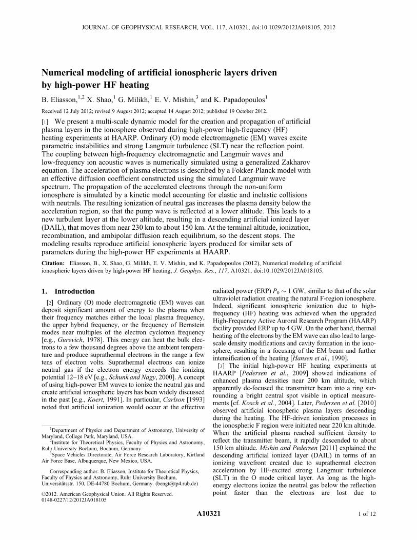
2 sin2 c is the distancebetween the cutoffs of the O mode and upper hybrid wave,and l0 is the vacuum wavelength of the EM wave. Forour parameters, with Ln = 43 km, Y = 0.4, c = 14� and l0 =100 m, we obtain d = 400 m and T = 10�29, which is neg-ligible. On the other hand, after the instability has beentaking place and SLT has created small-scale density fluc-tuations, the mode conversion is much more efficient.Figure 1 shows the simulation results for a pump waveamplitude EO ¼ 1:5 V=m and the ion (electron) temperatureTi = 0.2 eV (Te = 0.4 eV). Clearly, intense electrostaticwaves (the z component Ez) and ion density fluctuationsni are generated near the turning point zO = 230.6 km. Notethe different scales for Ex,y and Ez. The traces above 230 kmare due to the partial conversion into the Z mode, which forthe given conditions can propagate to the topside and gen-erate electrostatic turbulence near the transformation point[e.g., Mjølhus, 1990].[8] The large-amplitude z-component of the electric field
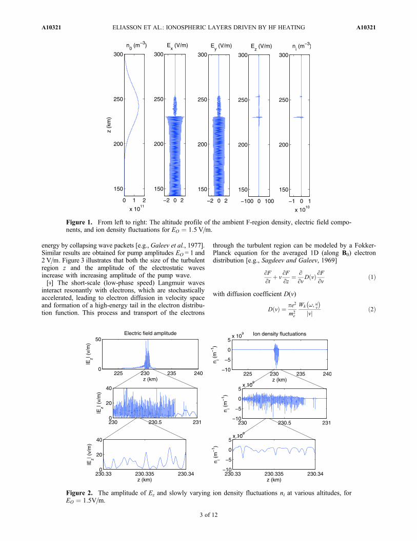
near zO appears due to the development of SLT near zO,which is manifested by solitary wave packets trapped in iondensity cavities [e.g., DuBois et al., 1990; Mjølhus et al.,2003]. Figure 2 shows the spatial structure of the electricfield and density in the vicinity of zO. The solitary waves andcavities of widths ds ≈ (15 � 25)rD ≈ 0.3–0.5 m are spacedapart by dls ≈ 1–2 m (rD ≈ 2 cm is the Debye radius). Whilethe O mode continues to pump energy, the system reaches adynamic equilibrium between the long-scale pumping andshort-scale absorption due to nonlinear transfer of the wave
ELIASSON ET AL.: IONOSPHERIC LAYERS DRIVEN BY HF HEATING A10321A10321
2 of 12
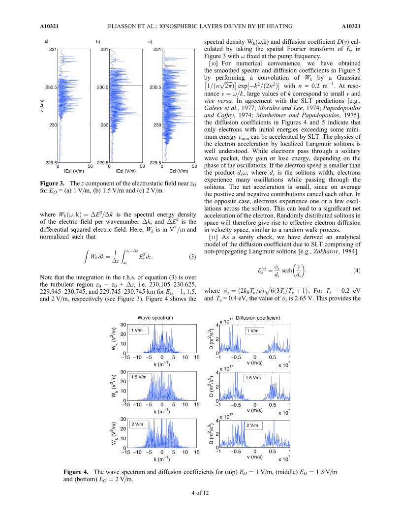
energy by collapsing wave packets [e.g., Galeev et al., 1977].Similar results are obtained for pump amplitudes EO = 1 and2 V=m. Figure 3 illustrates that both the size of the turbulentregion z and the amplitude of the electrostatic wavesincrease with increasing amplitude of the pump wave.[9] The short-scale (low-phase speed) Langmuir waves
interact resonantly with electrons, which are stochasticallyaccelerated, leading to electron diffusion in velocity spaceand formation of a high-energy tail in the electron distribu-tion function. This process and transport of the electrons
through the turbulent region can be modeled by a Fokker-Planck equation for the averaged 1D (along B0) electrondistribution [e.g., Sagdeev and Galeev, 1969]
∂F∂t
þ v∂F∂z
¼ ∂∂v
D vð Þ ∂F∂v
ð1Þ
with diffusion coefficient D(v)
D vð Þ ¼ pe2
m2e
Wk w; wv� �vj j ð2Þ
Figure 1. From left to right: The altitude profile of the ambient F-region density, electric field compo-nents, and ion density fluctuations for EO ¼ 1:5 V=m.
Figure 2. The amplitude of Ez and slowly varying ion density fluctuations ni at various altitudes, forEO ¼ 1:5V=m.
ELIASSON ET AL.: IONOSPHERIC LAYERS DRIVEN BY HF HEATING A10321A10321
3 of 12
where Wk w; kð Þ ¼ DE2=Dk is the spectral energy densityof the electric field per wavenumber Dk, and DE2 is thedifferential squared electric field. Here, Wk is in V2=m andnormalized such that
ZWk dk ¼ 1
Dz
Z z0þDz
z0
E2z dz: ð3Þ
Note that the integration in the r.h.s. of equation (3) is overthe turbulent region z0 � z0 + Dz, i.e. 230.105–230.625,229.945–230.745, and 229.745–230.745 km for EO = 1, 1.5,and 2 V=m, respectively (see Figure 3). Figure 4 shows the
spectral density Wk(w,k) and diffusion coefficient D(v) cal-culated by taking the spatial Fourier transform of Ez inFigure 3 with w fixed at the pump frequency.[10] For numerical convenience, we have obtained
the smoothed spectra and diffusion coefficients in Figure 5by performing a convolution of Wk by a Gaussian1=ðk ffiffiffiffiffiffi
2pp Þ� �
exp �k2=ð2k2Þ½ � with k = 0.2 m�1. At reso-nance v ¼ w=k, large values of k correspond to small v andvice versa. In agreement with the SLT predictions [e.g.,Galeev et al., 1977; Morales and Lee, 1974; Papadopoulosand Coffey, 1974; Manheimer and Papadopoulos, 1975],the diffusion coefficients in Figures 4 and 5 indicate thatonly electrons with initial energies exceeding some mini-mum energy ɛmin can be accelerated by SLT. The physics ofthe electron acceleration by localized Langmuir solitons iswell understood. While electrons pass through a solitarywave packet, they gain or lose energy, depending on thephase of the oscillations. If the electron speed is smaller thanthe product dsw, where ds is the solitons width, electronsexperience many oscillations while passing through thesolitons. The net acceleration is small, since on averagethe positive and negative contributions cancel each other. Inthe opposite case, electrons experience one or a few oscil-lations across the soliton. This can lead to a significant netacceleration of the electron. Randomly distributed solitons inspace will therefore give rise to effective electron diffusionin velocity space, similar to a random walk process.[11] As a sanity check, we have derived an analytical
model of the diffusion coefficient due to SLT comprising ofnon-propagating Langmuir solitons [e.g., Zakharov, 1984]
E sð Þz ¼ fs
dssech
z
ds
� �: ð4Þ
where fs ¼ 2kBTe=eð Þ ffiffiffiffiffiffiffiffiffiffiffiffiffiffiffiffiffiffiffiffiffiffiffiffiffiffiffiffi6 3Ti=Te þ 1ð Þp
. For Ti = 0.2 eVand Te = 0.4 eV, the value of fs is 2.65 V. This provides the
Figure 4. The wave spectrum and diffusion coefficients for (top) EO ¼ 1 V=m, (middle) EO ¼ 1:5 V=mand (bottom) EO ¼ 2 V=m.
Figure 3. The z component of the electrostatic field near zOfor EO = (a) 1 V=m, (b) 1:5 V=m and (c) 2 V=m.
ELIASSON ET AL.: IONOSPHERIC LAYERS DRIVEN BY HF HEATING A10321A10321
4 of 12
peak amplitude of ≈15–20 V=m for ds ≈ 0.13–0.20 m,consistent with the solitary wave packets in Figure 2. TheFourier transform of Ez
(s) in space
Ek ¼ffiffiffip2
rfs sech
pdsk2
� �ð5Þ
is normalized so that
ZE sð Þ2z dx ¼
ZE2k dk. Using an ensem-
ble of solitons, we can estimate the average spectral density
Wk ¼ NsE2k ¼
Nspf2s
2sech2
pdsk2
� �; ð6Þ
where Ns is the average number of solitons per meter. Thediffusion coefficient is
D vð Þ ¼ pe2
m2e
Wk w;w=kð Þvj j ¼ Nsp2e2
2m2e vj j
f2s sech
2 pdsw2v
� �: ð7Þ
In agreement with the above discussion, D(v) vanishes at|v| ≪ dsw, when the net acceleration is supposed to be small.The input parameters of the analytical model are Ns, ds, andfs. As an example, we have plotted the diffusion coefficient(7) in Figure 5 (indicated with red, dashed lines) forfs = 2.65 V, Ns = 1.43 m�1 and ds = 1.19 m. It is seen thatthe analytical model is fairly close to the simulations atvj j ≤ 6� 106 m=s or energy ɛ ¼ mev2=2 ≤ 100 eV and sig-nificantly deviates only at ɛ > 100 eV for EO ¼1:5 and 2 V=m. Therefore, we conclude that the analyticmodel satisfactorily describes acceleration of the most sig-nificant part of the suprathermal electron population.
[12] Next, the convolved diffusion coefficients (such as inFigure 5) are used to solve equation (1) at various tempera-tures of the ambient electrons. The computational domain invelocity space is from �107 m/s to +107 m/s, resolved by400 intervals, and in z-domain set by the width of the tur-bulent region (typically about 500 m to 1 km; see Figure 5),and resolved by 10 intervals. The solution is advanced in timewith the standard 4th-order Runge-Kutta scheme with the timestep 5 � 10�9 s. The ambient population is assumed Maxwel-lian with the distribution FM ¼ 1=
(bottom) boundary, we use an inflow condition for negative(positive) velocities and an outflow condition for positive(negative) velocities. As an inflow condition, we set F = FM
on the boundary, and as an outflow condition at the oppositeboundary, we solve the Fokker-Planck equation (1) on theboundary. The electrons gain energy as they travel throughthe turbulent region. After some time, the equilibriumbetween inflow, outflow, and electron acceleration is estab-lished. Figure 6 shows the resulting electron distribution as afunction of velocity and altitude. Electrons with negativevelocities (v < 0) flow downwards and are gradually heated,resulting in a widening of the electron distribution functionfor negative velocities at the bottom boundary, and vice versafor electrons with positive velocities (v > 0) streamingupwards. This leads to an asymmetric electron distributionwith high-energy tails streaming out from the heated region.It is clear from Figure 6 that only electrons with a largeenough initial temperatures of about 0.4 eV and above areefficiently heated by the turbulence, while the electronswith temperature 0.2 eV are only slightly heated by theturbulence.[13] To assess the validity of the Fokker-Planck scheme,
we have compared it with direct test particle simulations,
Figure 5. The convolved wave spectra and diffusion coefficients for EO = (top) 1 V=m, (middle) 1:5 V=m,and (bottom) 2 V=m. The red dashed lines indicate the results of the analytical model (7) with the fittedcoefficients Ns = 1.43 m�1 and ds = 1.19 m.
ELIASSON ET AL.: IONOSPHERIC LAYERS DRIVEN BY HF HEATING A10321A10321
5 of 12
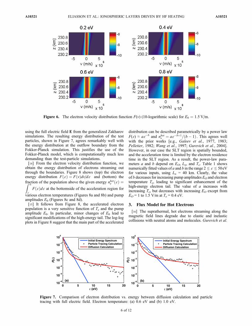
using the full electric field E from the generalized Zakharovsimulations. The resulting energy distribution of the testparticles, shown in Figure 7, agrees remarkably well withthe energy distribution at the outflow boundary from theFokker-Planck simulation. This justifies the use of theFokker-Planck model, which is computationally much lessdemanding than the test-particle simulations.[14] From the electron velocity distribution function, we
obtain the energy distribution of electrons streaming outthrough the boundaries. Figure 8 shows (top) the electronenergy distribution F ɛð Þ ¼ F vð Þdv=dɛ and (bottom) thefraction of the population above the given energy nhote ɛð Þ ¼Z ∞
ɛF ɛð Þdɛ at the bottomside of the acceleration region for
various electron temperatures (Figures 8a and 8b) and pumpamplitudes E0 (Figures 8c and 8d).[15] It follows from Figure 8, the accelerated electron
population is a very sensitive function of Te and the pumpamplitude E0. In particular, minor changes of E0 lead tosignificant modifications of the high-energy tail. The log-logplots in Figure 8 suggest that the main part of the accelerated
distribution can be described parametrically by a power lawF(ɛ) ≈ aɛ�b and nhote ¼ aɛ�bþ1=ðb� 1Þ . This agrees wellwith the prior works [e.g., Galeev et al., 1977, 1983;Pelletier, 1982; Wang et al., 1997; Gurevich et al., 2004].However, in our case the SLT region is spatially bounded,and the acceleration time is limited by the electron residencetime in the SLT region. As a result, the power-law para-meters a and b depend on EO, Ln, and Te. Table 1 showsnumerically fitted values of a and b in the range 2 ≤ ɛ ≤ 50eVfor various inputs, using Ln = 40 km. Clearly, the valueof b decreases for increasing pump amplitudes EO and electrontemperature Te, leading to significant enhancement of thehigh-energy electron tail. The value of a increases withincreasing Te, but decreases with increasing EO except fromEO = 1 to 1.5 V/m at Te = 0.4 eV.
3. Flux Model for Hot Electrons
[16] The suprathermal, hot electrons streaming along themagnetic field lines degrade due to elastic and inelasticcollisions with neutral atoms and molecules. Gurevich et al.
Figure 6. The electron velocity distribution function F(v) (10-logarithmic scale) for E0 ¼ 1:5 V=m.
Figure 7. Comparison of electron distribution vs. energy between diffusion calculation and particletracing with full electric field. Electron temperature: (a) 0.6 eV and (b) 1.0 eV.
ELIASSON ET AL.: IONOSPHERIC LAYERS DRIVEN BY HF HEATING A10321A10321
6 of 12
[1985] showed that their distribution outside a thin acceler-ating layer can be approximated as
Fhot ɛ; zð Þ ¼ F ɛð Þ exp �Z z
zo
dz
L z; ɛð Þ� �
; ð8Þ
where the collisional loss length L(z,ɛ) is given by
and F(ɛ) is obtained from the acceleration model (in theprevious section) as a boundary condition at z = z0. Herestr
j is the transport cross-section for elastic collisions andsin
j is the cross-section for inelastic collisions with neutralspecies j.[17] Figure 9 shows the energy spectra of the fast electrons
at various altitudes above (Figure 9a) and below (Figure 9b)the acceleration region near z0 = 230 km for EO ¼ 1:5 V=mand the ambient electron temperature Te0 = 0.6 eV. Note thedifferent scales for F(ɛ) in Figures 9a and 9b. As anticipated,the fast electrons rapidly degrade below z0 due to inelasticlosses increasing along with the neutral density.
4. Descending Artificial Ionized Layer (DAIL)
[18] A model of the development of newly ionized (arti-ficial) plasma involves the spatial and temporal evolution ofionospheric electrons and four ion species, O+, NO+, O2
+, andN2+. The main chemical processes included in the model are
ionization of atomic and molecular oxygen and nitrogen bythe accelerated electrons, production of molecular oxygenions and nitrogen monoxide ions via charge exchange col-lisions, O+ + O2 → O2
+ + O and O+ + N2 → NO+ + N,respectively, and recombination between electrons and
molecular ions [e.g., Schunk and Nagy, 2000]. The resultingsystem of equations includes
∂n∂t
¼ kionNn1
n0e� n
nNOþ
tNOþrec
� nnOþ
2
tOþ2
rec
� nnNþ
2
tNþ2
rec
� n
tdð10Þ
∂nOþ
∂t¼ kOionNO
1
n0e� nOþ
t 1ð Þexc
� nOþ
t 2ð Þexc
� nOþ
tdð11Þ
∂nNOþ
∂t¼ nOþ
t 1ð Þexc
� nnNOþ
tNOþrec
� nNOþ
tdð12Þ
∂nOþ2
∂t¼ kO2
ionNO2
1
n0eþ nOþ
t 2ð Þexc
� nnOþ
2
tOþ2
rec
�nOþ
2
tdð13Þ
∂nNþ2
∂t¼ kN2
ionNN2
1
n0e� n
nNþ2
tNþ2
rec
�nNþ
2
tdð14Þ
Figure 8. (top) The electron energy distribution F(ɛ) and (bottom) the fraction of the population abovethe given energy ne
hot(ɛ) for various (a and b) Te and (c and d) E0.
Table 1. Fitted Power Law Coefficients a and b as Functions ofE0 and Te
and b2 ¼ 2:1� 10�11 cm3=s [Schunk and Nagy, 2000].[19] Plasma decay due to ambipolar diffusion is accounted
for by including the terms with the decay time td ¼L2N=DA in the right-hand side of the system (10)–(14).Here DA ¼ 1þ Te=Tið ÞkBTi=minin is the ambipolar diffu-sion coefficient, nin = CinNn, Nn = NO + NO2
+ NN2is the
total neutral density, and LN ¼ 1=ðd ln Nn=dzÞ is thelength-scale of the neutral gas. For simplicity, Cin ¼4� 10�10 cm�3=s is taken for all ion species. The totalionization rate for electrons kionNn = kion
O NO + kionO2NO2
+kionN2 NN2
defines the ionization time scale tion ¼ ne=ðkionNnÞ.
Figure 9. The electron energy distribution Fhot(ɛ,z) at various altitudes (a) above and (b) below the accel-eration region for EO ¼ 1:5 V=m and Te0 = 0.6 eV.
Figure 10. The diffusion, ionization, recombination, and charge exchange times vs. altitude for theacceleration region at z0 = 230 km, EO ¼ 1:5 V=m, and Te0 = 0.6 eV.
ELIASSON ET AL.: IONOSPHERIC LAYERS DRIVEN BY HF HEATING A10321A10321
[20] Figure 10 shows the time scales for ionization,recombination, charge exchange collisions, and diffusion asfunctions of altitude calculated below the acceleration regionnear z0 = 230 km using Fhot(ɛ, z) from Figure 9b. The ion-ization rate � 1=tion decreases dramatically at lower alti-tudes due to the rapid degradation of the fast electronpopulation, as seen in Figure 9b. This limits the region of thenewly produced (artificial) plasma by the average degrada-tion length of the ionizing (ɛ > ɛ j
ion) fast electrons.
[21] The solution of the system (10)–(15) is consistentwith the Mishin and Pedersen [2011] ionizing wavefrontscenario. The SLT acceleration region (layer) is located justbelow the turning point zO of the pump wave defined by thematching of the pump frequency to the local plasma fre-quency or ne = nc. As the new plasma builds up, thematching condition is reached somewhere at z = zs < zOdefined by the matching condition ne(zs) = nc. Then, SLTdevelops within the new layer, and the aforesaid accelera-tion/ionization process is repeated again and again, everytime at lower altitudes adjacent to zs(t). In the simulation,a 4th-order Runge-Kutta scheme for the time stepping is
Figure 12. (a) Scaling of the final DAIL position and (b) average descent speed vs. injected wave ampli-tude for three different initial electron temperatures.
Figure 11. Time-vs-altitude plots of the densities in cm�3 of (a) electrons, (b) O+ ions, (c) N2+ ions, and
(d) O2+ ions, for EO ¼ 1:5 V=m, and Te0 = 0.6 eV.
ELIASSON ET AL.: IONOSPHERIC LAYERS DRIVEN BY HF HEATING A10321A10321
9 of 12
applied with a 0.1 s time step and a spatial grid of 0.5 km.The location of the accelerating layer, initially at 230 km, isdynamically updated at each time step. We assume that SLTproduces the same power-law distribution at each step.[22] Figure 11 shows the temporal and spatial develop-
ment of the densities of electrons, O+ and molecular ions. Itis seen that in 4 minutes the artificial plasma descends from230 to ≈160 km with the mean speed ≈300 m=s. Initially, theelectron and O+ densities increase in step due to ionization ofmainly atomic oxygen, which is the dominant component atz > 180 km. At lower altitudes, the formation of the artificialplasma is dominated by ionization of nitrogen. The iono-spheric length scale Ln at the critical layer typically decrea-ses from about 40 km in the original ionosphere, to about10 km at lower altitudes. Near the terminal altitude of150 km, the ionization production (cf. Figure 10) and speedof descent slow down. At the terminus, the ionization pro-duction is balanced mainly by recombination of molecularions, and the descent stops.[23] Figure 12 shows the DAIL terminal altitude
(Figure 12a) and the average descent speed (Figure 12b)computed for different values of EO and Te0. The averagespeed is simply the distance from the initial altitude to theterminus divided by the propagation time. At relatively lowEO ¼ 1 V=m and Te0 = 0.2 eV, the DAIL descends by lessthan 10 km. For lower pump electric fields and electrontemperatures, DAILs do not develop. As anticipated fromthe dependence of the ionization rate, the average speedincreases with EO and Te0.[24] To compare directly with the DAIL optical sig-
natures [Pedersen et al., 2010], the green-line emissionshave been calculated from the simulation data. As in theexperiment, the green-line emission serves as diagnostics
of the related DAIL. Figure 13 shows the results ofmodeling of the relative intensity of the oxygen emissionat 557.7 nm (the green line) excited by the acceleratedelectrons. The emission intensity I is proportional to theexcitation rate of atomic oxygen by the electron impact
I ∝ NO
Z ∞
4:2 eVFhot ɛ; zð Þs1S ɛ; zð Þv ɛð Þdɛ. Here ss is the
excitation cross section of the O(1S) state. As with thedescent speed, the intensity increases with the pumpelectric field and the temperature of the bulk of electrons.
5. Discussion
[25] In this section, we compare the simulation resultswith the observed features of HF-induced plasma layers. Thesimulations produce an artificial ionospheric layer, des-cending from ≈230 km on average at ≈300 m/s, until ioni-zation is balanced by recombination and ambipolar diffusionnear 150 km. As it follows from Figure 11a, during the first2 min in the heating, the O+-dominated newly born plasmaat h ≥ 180 km is confined to the bottomside of the original F2layer. At lower altitudes, the artificial plasma above thedescending acceleration-ionization source is rapidlydepleted due to recombination of molecular ions, therebyseparating the ionization front from the original F2 peak.These features agree well with the Pedersen et al. [2010]ionosonde and optical observations. The correspondingdescent of the SLT generation region is also observed by theMUIR radar ion-line observations [Mishin and Pedersen,2011, Figure 1].[26] The low-amplitude threshold of EO for the formation
of DAILs seen in Figure 12a is in line with the recentobservations at HAARP [Pedersen, 2012] which show that
Figure 13. Green line emission as derived from simulation for different input wave amplitude and initialelectron thermal energy: (a) E0 = 1 V/m, Te = 0.4 eV, (b) E0 = 1.5 V/m, Te = 0.4 eV, and (c) E0 = 1 V/m,Te = 0.6 eV.
ELIASSON ET AL.: IONOSPHERIC LAYERS DRIVEN BY HF HEATING A10321A10321
10 of 12
DAILs have a threshold that appears to be somewherebetween 1/3 and 1/2 HAARP full power, and under rela-tively low-amplitude electric fields, weak DAILs are formedslightly below the heating wave reflection point.[27] On the other hand, Figure 12b revealed that the
average descent speed of the DAIL increases with theinjected electric field and the temperature of the bulk ofelectrons. Mishin and Pedersen [2011] showed that in theirexperiments the average descent speed was about 0.3 km/s.In our model this value corresponds to the field rangebetween 1.1–1.4 V/m while the electron temperature rangesbetween 0.6–0.4 eV. A descent speed of 0.3 km/s alsooccurs at electron temperatures as low as 0.2 eV when theelectric field is about 1.8 V/m. This provides an estimate forthe range of parameters required to form DAILs such asobserved at HAARP.[28] We conclude that the salient observational features of
the artificial plasma layers are well reproduced by the sim-ulated ionization front created by the SLT-accelerated elec-tron population. However, the observed and modeledionospheric length scales Ln differ significantly at h < 180 km.The cause of that is the assumption that at each step the samedistribution is produced. At low altitudes, as noted byMishinand Pedersen [2011], the maximum energy of the acceleratedelectrons can be limited by inelastic losses that peak atɛ = ɛmax < 100 eV. For the ionization layer to stop des-cending, the total rate of inelastic collisions vil ɛmaxð Þ ≅ 3�10�7Nn
ffiffiffib
p= b þ 8ð Þ b ¼ ɛ=ɛ ionð Þ should exceed the accel-
eration rate of fast electrons ga�D(vmax)/vmax2 [Volokitin and
Mishin, 1979]. Indeed, with D(v) from Figure 5 for EO ¼1V=m we obtain that vil > ga at Nn > 3 � 1010 cm�3, i.e.below about 160 km. Further, the pump amplitudes EO ≥1 V/m and electron temperatures Te ≥ 0.4 eV have been usedto obtain the accelerated electron population. The enhancedTe near the turning point zO can be produced jointly byheating of ionospheric electrons directly by SLT and viafast electron thermal conduction from the upper hybridlayer [cf. Pedersen et al., 2010]. However, the electrontemperature is probably still too low for direct ionization dueto bulk heating. Only electrons above a critical energy of aboutɛc = 12 eV will contribute to the ionization. Integrating theMaxwellian electron distribution function for energiesabove this value, we obtain the fraction of the electron pop-ulation above the critical energy as dne ɛcð Þ ≈ ffiffiffiffiffiffiffiffiffiffiffiffiffiffiffiffiffiffiffiffi
2ɛc=ðpTeÞp
exp [�ɛc=ð2TeÞ]. To obtain dne(ɛc) > 10�3 (a typical fractionproduced by SLT), we need an electron temperature Te above1.5 eV, which is a few times higher than the values observedin the experiments. The remaining question is the value ofEO. The free-space electric field of the injected pump wave isEO ≈ 5:5
ffiffiffiffiffiP0
p=R V/m at the effective radiative power P0 (in
MW) and distance R (in km). For R = 200 km, EO reaches≈1 V/m at P0 ≈ 2.3 GW, which is near the maximum for theupgraded HAARP transmitter at f0 ≈ 7 MHz. However, arti-ficial layers [Pedersen et al., 2010] have been observed atf0 = 2.85 MHz and P0 ≈ 440 MW. A simple resolution tothis quandary is accounting for background (“seed”) supra-thermal electrons, e.g., photoelectrons that can be acceleratedmuch more efficiently than thermal electrons [e.g., Mishinet al., 2004]. As soon as the ionizing front is established,the seed electron population near zs will be maintained viadegradation of the earlier-accelerated electrons streaming
downward from zs. We are currently expanding the codein order to include background suprathermal electrons intoSLT acceleration and the pump fields increasing at loweraltitudes with 1=R.[29] In summary, we have presented a multi-scale model
for the generation and descent of artificial layers by high-power HF radio waves recently observed at HAARP. Themodel includes a complete wave model of the ionosphericturbulence, from which an effective diffusion coefficient isderived and used in a Fokker-Planck model for electronacceleration due to resonant wave-particle interactions. Thetransport of the hot electrons is modeled with a kineticmodel, and a dynamic model is developed to describe thecreation and descent of the artificial ionospheric layers.
[30] Acknowledgments. The work at UMD was supported byDARPA via a subcontract N684228 with BAE Systems and also by MURIN000140710789. E.V.M. was supported by the Air Force Office of Scien-tific Research. B.E. acknowledges partial support by the DFG FOR1048(Bonn, Germany).[31] Robert Lysak thanks the reviewers for their assistance in evaluat-
ing this paper.
ReferencesCarlson, H. C., Jr. (1993), High-power HF modification: Geophysics, spanof EM effects, and energy budget, Adv. Space Res., 13(10), 15–24,doi:10.1016/0273-1177(93)90046-E.
DuBois, D. F., H. A. Rose, and D. Russell (1990), Excitation of strongLangmuir turbulence in plasmas near critical density: Application to HFheating of the ionosphere, J. Geophys. Res., 95, 21,221–21,272,doi:10.1029/JA095iA12p21221.
Eliasson, B. (2008a), A nonuniform nested grid method for simulationsof RF induced ionospheric turbulence, Comput. Phys. Commun., 178,8–14, doi:10.1016/j.cpc.2007.07.008.
Eliasson, B. (2008b), Full-scale simulation study of the generation oftopside ionospheric turbulence using a generalized Zakharov model,Geophys. Res. Lett., 35, L11104, doi:10.1029/2008GL033866.
Eliasson, B., and L. Stenflo (2008), Full-scale simulation study of theinitial stage of ionospheric turbulence, J. Geophys. Res., 113, A02305,doi:10.1029/2007JA012837.
Eliasson, B., and L. Stenflo (2010), Full-scale simulation study of electro-magnetic emissions: The first ten milliseconds, J. Plasma Phys., 76,369–375, doi:10.1017/S0022377809990559.
Galeev, A. A., R. Z. Sagdeev, V. D. Shapiro, and V. I. Shevchenko (1977),Langmuir turbulence and dissipation of high-frequency energy, Sov.Phys. JETP, Engl. Transl., 46, 711–728.
Galeev, A., R. Sagdeev, V. Shapiro, and V. Shevehenko (1983), Beamplasma discharge and suprathermal electron tails, in Active Experimentsin Space (Alpbach, Austria), Eur. Space Agency Spec. Publ., ESA SP-195,151–155.
Gurevich, A. (1978), Nonlinear Phenomena in the Ionosphere, Springer,New York, doi:10.1007/978-3-642-87649-3.
Gurevich, A. V., Y. S. Dimant, G. M. Milikh, and V. V. Vas’kov (1985),Multiple acceleration of electrons in the regions of high-power radio-wavereflection in the ionosphere, J. Atmos. Terr. Phys., 47, 1057–1070,doi:10.1016/0021-9169(85)90023-6.
Gurevich, A. V., H. C. Carlson, Y. V. Medvedev, and K. P. Zybin (2004),Langmuir turbulence in ionospheric plasma, Plasma Phys. Rep., 30,995–1005, doi:10.1134/1.1839953.
Hansen, J. D., G. J. Morales, L. M. Duncan, J. E. Maggs, and G. Dimonte(1990), Large-scale ionospheric modifications produced by nonlinearrefraction of an hf wave, Phys. Rev. Lett., 65, 3285–3288, doi:10.1103/PhysRevLett.65.3285.
Koert, P. (1991), Artificial ionospheric mirror composed of a plasma layerwhich can be tilted, Patent 5,041,834, U.S. Patent and Trademark Off.,Washington, D. C.
Kosch, M. J., M. T. Rietveld, A. Senior, I. W. McCrea, A. J. Kavanagh,B. Isham, and F. Honary (2004), Novel artificial optical annular struc-tures in the high latitude ionosphere over EISCAT, Geophys. Res. Lett.,31, L12805, doi:10.1029/2004GL019713.
Manheimer, W. M., and K. Papadopoulos (1975), Interpretation of solitonformation and parametric instabilities, Phys. Fluids, 18, 1397–1398,doi:10.1063/1.861003.
ELIASSON ET AL.: IONOSPHERIC LAYERS DRIVEN BY HF HEATING A10321A10321
11 of 12
Mjølhus, E. (1990), On linear conversion in a magnetized plasma, RadioSci., 25, 1321–1339, doi:10.1029/RS025i006p01321.
Mjølhus, E., E. Helmersen, and D. DuBois (2003), Geometric aspects ofHF driven Langmuir turbulence in the ionosphere, Nonlinear ProcessesGeophys., 10, 151–177, doi:10.5194/npg-10-151-2003.
Mishin, E., and T. Pedersen (2011), Ionizing wave via high-power HFacceleration,Geophys. Res. Lett., 38, L01105, doi:10.1029/2010GL046045.
Mishin, E. V., W. J. Burke, and T. Pedersen (2004), On the onset ofHF-induced airglow at HAARP, J. Geophys. Res., 109, A02305,doi:10.1029/2003JA010205.
Morales, G. J., and Y. C. Lee (1974), Effect of localized electric fields onthe evolution of the velocity distribution function, Phys. Rev. Lett., 33,1534–1537, doi:10.1103/PhysRevLett.33.1534.
Papadopoulos, K., and T. Coffey (1974), Nonthermal features of the auroralplasma due to precipitating electrons, J. Geophys. Res., 79, 674–677,doi:10.1029/JA079i004p00674.
Pedersen, T. (2012), Artificial ionospheric layers: Recent progress andpropagation effects, paper presented at RF Ionospheric InteractionsWorkshop, Natl. Sci. Found., Santa Fe, N. M., April.
Pedersen, T., B. Gustavsson, E. Mishin, E. MacKenzie, H. C. Carlson,M. Starks, and T. Mills (2009), Optical ring formation and ionizationproduction in high-power HF heating experiments at HAARP, Geophys.Res. Lett., 36, L18107, doi:10.1029/2009GL040047.
Pedersen, T., B. Gustavsson, E. Mishin, E. Kendall, T. Mills, H. C. Carlson,and A. L. Snyder (2010), Creation of artificial ionospheric layers usinghigh-power HF waves, Geophys. Res. Lett., 37, L02106, doi:10.1029/2009GL041895.
Pelletier, G. (1982), Generation of a high-energy electron tail by strongLangmuir turbulence in plasma, Phys. Rev. Lett., 49, 782–785,doi:10.1103/PhysRevLett.49.782.
Sagdeev, R., and A. Galeev (1969), Nonlinear Plasma Theory, Benjamin,New York.
Schunk, R.W., andA.N. Nagy (2000), Ionospheres - Physics, Plasma Physicsand Chemistry, Cambridge Univ. Press, New York, doi:10.1017/CBO9780511551772.
Volokitin, A., and E. Mishin (1979), Relaxation of an electron beam in aplasma with infrequent collisions, Sov. J. Plasma Phys., 5, 654–656.
Wang, J., D. Newman, and M. Goldman (1997), Vlasov simulations ofelectron heating by Langmuir turbulence near the critical altitude inthe radiation-modified ionosphere, J. Atmos. Sol. Terr. Phys., 59,2461–2474, doi:10.1016/S1364-6826(96)00140-X.
Zakharov, V. (1984), Collapse and self-focusing of Langmuir waves, inBasic Plasma Physics, vol. 2, edited by A. Galeev and R. Sudan,pp. 81–121, North-Holland, New York.
ELIASSON ET AL.: IONOSPHERIC LAYERS DRIVEN BY HF HEATING A10321A10321


![Artificial ionospheric layers driven by high-frequency ...nlpc.stanford.edu/nleht/Science/articles/Mishin+2016_10...[e.g.,Mishin et al.,2000].Inturn,thelocationofthespectralpeaksisstilldefinedbytheionsoundfre-quencyf](https://static.documents.pub/doc/80x56/5abff29c7f8b9a5a4e8b6408/artificial-ionospheric-layers-driven-by-high-frequency-nlpc-201610egmishin.jpg)


