The Pennsylvania State University The Graduate School College of Earth and Mineral Sciences NUMERICAL MODELING OF NATURAL GAS TWO-PHASE FLOW SPLIT AT BRANCHING T-JUNCTIONS WITH CLOSED-LOOP NETWORK APPLICATIONS A Dissertation in Petroleum and Natural Gas Engineering by Doruk Alp c 2009 Doruk Alp Submitted in Partial Fulfillment of the Requirements for the Degree of Doctor of Philosophy December 2009
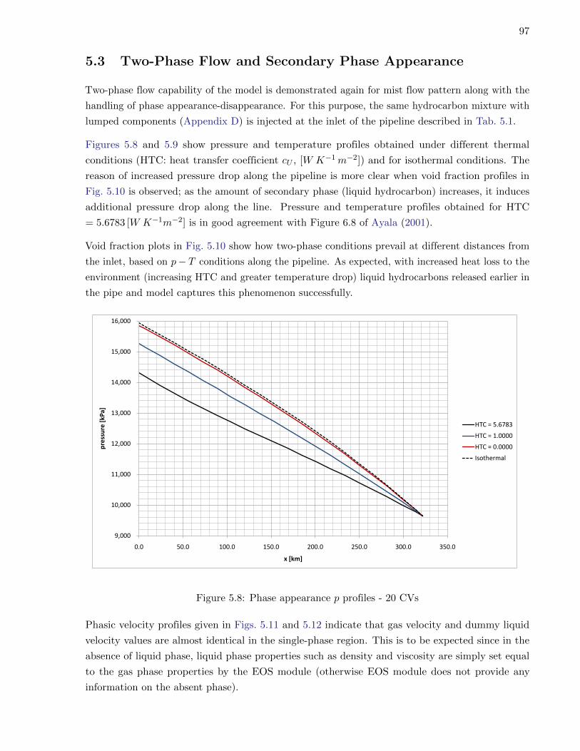
Transcript
The Pennsylvania State University
The Graduate School
College of Earth and Mineral Sciences
NUMERICAL MODELING OF NATURAL GAS TWO-PHASE FLOW SPLIT
K Mechanical energy loss coefficient [dimensionless]
p Pressure [Pa]
Re Reynolds number [dimensionless]
q Volumetric flow rate [m3 s−1]
Q Pipe heat input [J m−2]
si Interfacial area, flow pattern dependent si = ωi∆x [m2]
swL Pipe area wetted by liquid, flow pattern dependent swL = ωL∆x [m2]
T Temperature [K]
T∞ Surrounding (ambient) temperature [K]
u Superficial velocity [ms−1]
v Velocity [ms−1]
V Volume [m3]
z Elevation [m]
Z Gas compressibility factor [dimensionless]
Greek letters:
αG Void fraction [dimensionless]
αL Holdup [dimensionless]
β T-junction branching angle [rad]
δk Distance of phase k from pipe wall [m]
x
ε Pipe roughness [m]
η Joule-Thomson coefficient [K Pa−1]
γG Gas gravity (or gas specific gravity) [dimensionless]
ΓG Rate of mass transfer from liquid-to-gas phase, per unit volume of CV, negative for
condensation and positive for evaporation [kgm−3 s−1]
ΓL Rate of mass transfer from gas-to-liquid phase, per unit volume of CV, positive for
condensation and negative for evaporation [kgm−3 s−1]
λ Branch to inlet mass intake ratio [dimensionless]
Λ Phasic volume fraction [dimensionless]
ωi Phasic interface wetted perimeter [m]
ωL Liquid wetted perimeter [m]
φk Phasic flow multiplier [dimensionless]
φ1 Heat transfer factor [m−1]
φ2 Potential and kinetic energy factor [Km−1]
Φ Two-phase loss multiplier [dimensionless]
ρ Density [kgm−3]
τi Interfacial stress [N m−2]
τw Pipe wall shear [N m−2]
θ Pipe inclination [rad]
σ Radial angle for zone of influence on pipe cross-section [rad]
Subscript:
G Gas phase
L Liquid phase
irr Irreversible
rev Reversible
xi
Acknowledgements
I would like to begin by expressing my deepest gratitude to my advisor Dr.Luis Ayala for bringing
me to Penn State and for his financial support. Needless to say, the four years I have been at Penn
State has been a totally life changing experience which has opened such a path for me that I could
not have thought of otherwise. For this great opportunity, many things I have learned from him and
through the course of this research that have fundamentally changed my understanding of numerical
modeling; for his guidance, understanding and patience with me; I am forever in his debt.
I am truly grateful to Dr.John Mahaffy from whom I have learned a great deal on the subject;
through two courses I took from him and our discussions, as well as additional references he provided
me with during early stages of the study. To a large extend, the approach taken in the study is
based on my learnings from him.
I would like to thank the committee members Dr.Turgay Ertekin, Dr.Robert Watson and Dr.Mirna
Macdonald for their time, interest in the study, valuable comments and input.
I would like to extend my special thanks to Dr.Turgay Ertekin for his understanding, support and
guidance through these years.
I would also like to thank EME staff assistants, and Penn State staff in general, for making my stay
smooth and free of obstacles.
Finally, I would like to express my deep gratitude to my parents Zerrin and Mustafa Alp for their
understanding, continuous and unconditional support overseas through these four years. Their
emotional support and financial assurance has always put my mind at ease and allowed me to focus
my full attention on my studies. As always, I am in their debt.
xii
1
Chapter 1
Introduction
Gaseous hydrocarbon mixtures are brought from wellheads to surface facilities via ‘gathering’ pipe
systems. After necessary treatment, natural gas is delivered to industrial or residential customers
several hundred kilometers away via ‘transmission’ pipelines. Main transmission lines are connected
to a ‘distribution’ grid at the gates of cities or industrial zones. Hence, from wellbore to the end
consumer, natural gas is delivered via complex and integrated network of pipes.
Two-phase flow of hydrocarbon mixtures in a network of pipes could be either a deliberate choice of
the operator or a result of inevitable flow conditions; such as ‘retrograde condensation’ of heavier
hydrocarbons in the case of natural gas lines. Two-phase flow is typically expected in the wellbore
and through out the surface gathering system when oil and gas, water and gas, or oil and water are
initially present and produced simultaneously from the reservoir. On the other hand, depending
on reservoir type, production stage and wellbore conditions liquid hydrocarbons (or water) may
condense in the pipeline as the second phase (or water may condense as the third phase, i.e. water
in emulsion with liquid hydrocarbons); even if inlet stream is single phase.
For on-shore operations, once separation and treatment is completed in centralized facilities close to
well sites, it is preferred to transport oil and gas in separate lines, as single phase fluids. In off-shore
operations, space limitations might impose a need for simultaneous transportation of oil and gas to
on-shore facilities located a considerable distance from the well site.
Branching T-junctions are essential components of small and large scale piping systems found in nat-
ural gas and oil pipeline networks, as well as various industrial applications. Two-phase flow through
branching tees (T-junctions) result in pronounced hydraulic losses and uneven phase separation
following the split of flow stream; ultimately causing profound effects on system performance and
quality of delivered fluids. Furthermore, for the practical purposes of system design and analysis,
almost all other types of junctions joining three or more pipes, as well as specialized sink/source
terms such as wellheads or supply/demand nodes, could then be represented with appropriate
arrangement of consecutive three-arm junctions; in particular tees. Consequently, quantifying
two-phase flow associated hydraulic losses and phase separation through T-junctions is a matter of
serious concern for the design and analysis of various pipe systems.
Industrial applications where two-phase flow split is typically observed include:
• Two-phase flow of refrigerants through distribution headers of multi-pass evaporators or
2
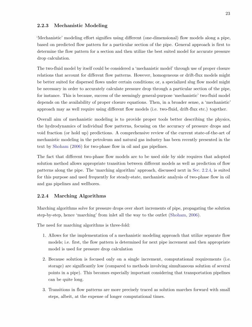
Figure 1.1: Branching T-junction
multi-system air-conditioners (Tae and Cho, 2006).
• Process plants where two-phase streams of chemicals, steam or air-water mixtures are delivered
to various locations in the plant via networks of pipes (Fouda and Rhodes, 1974).
• Conventional (fossil-fueled) power plants where steam is the ‘prime mover’.
• Nuclear reactor coolant loops of various design; i.e. pressurized (PWR), light (LWR) or boiling
(BWR) water reactors (Lahey, 1986) and associated small break discharge scenarios (Smoglie
et al., 1987). Two-phase flow is encountered within reactor coolant systems when water boils
due to large pressure drops; typically caused by accidental bursts of pipes in the primary
coolant loop, known as the loss of coolant accident (LOCA, Todreas and Kazimi, 1990).
• Circulation of geothermal fluids for heating purposes or transportation to geothermal power
plants via pipeline networks (Shoham, 2006).
• Steam injection networks for enhanced oil recovery (EOR) applications (Berger et al., 1997;
Jones and Williams, 1993).
• Condensate (water or liquid hydrocarbon) formation in natural gas gathering and transporta-
tion pipelines (Oranje, 1973).
• Functional phase separators and slug catchers for off-shore platforms and sea floor wellheads
(Margaris, 2007; Azzopardi and Rea, 2000).
It is important to note that through out this text, term ‘phase separation’ is distinctively used
to signify individual distribution of each incoming phase to the outgoing arms of a tee (Fig. 1.1),
while the term ‘phase distribution’ denotes the tendency of gas phase (void fraction) to occupy
certain parts of the pipe cross-section (e.g. due to gravity) –pronounced only in multidimensional
analysis because such details are lost with averaging in one-dimensional analysis (Lahey, 1990; cf.
Chapters 2 and 3). Finally, the term ‘phase split’ stands for the formation of the secondary phase
as a result of phase behavior response to changing pressure and temperature conditions.
In many industrial applications involving two-phase flow, formation of a lighter secondary phase (i.e.
gas) is expected, following a pressure drop in the flow stream that is initially all liquid. For instance,
3
gas phase evolves following pressure drops in oil pipelines. Hence, typically high liquid loading
conditions; i.e. predominantly liquid phase flow, is observed. On the other hand, condensation
of water in steam injection or distribution systems and formation of hydrocarbon liquids (the
condensate) in natural gas lines are low liquid loading conditions (predominantly gas phase flow)
where formation of an heavier secondary phase is observed (the liquid hydrocarbon).
In natural gas pipelines, according to gas composition, and particularly if heavier components are
abundant in the stream (i.e. wet gas), the phase envelope of the hydrocarbon mixture can partially
or entirely enclose the pipe operational region. If operational region is completely within the phase
envelope then two-phase flow would begin right at the very inlet of the system. If operational region
is partially enclosed by the phase envelope then two-phase flow is encountered in the sections of
pipe system where flowing pressure falls inside the phase envelope (Fig. 1.2).
Figure 1.2: Typical phase envelope for natural gases
Therefore, even though single phase conditions are prescribed at the inlet, and thus transportation
commences in entirely gaseous phase, (undersaturated) natural gases tend to drop hydrocarbon
liquids once pressure goes below hydrocarbon dew point conditions in the pipe. Thus, multi-phase
flow can prevail in natural gas transmission lines as well as gathering systems due to retrograde
condensation.
Simultaneous flow of natural gas and condensate is not efficient because presence of a secondary
phase (the condensate) decreases the deliverability of primary phase (gas), due to increased flow
(hydraulic) losses associated with decreased flow area available for the primary phase. Besides;
density, volume and calorific value of both phases vary along the pipeline as flow conditions change
because hydrocarbon phases in contact will continuously alter composition as a result of mass
transfer between the phases. Therefore, mass transfer and fluid re-distribution (i.e. phasic flow path
preference) in the pipeline network have significant influence on fluid and flow properties as well as
overall system performance.
There are two parts to the analysis of two-phase flow problem associated with condensate formation
in natural gas pipelines:
• Prediction and modeling of two-phase flow in straight sections of the network.
4
• Calculation of flow (hydraulic) losses and phase separation at T-junctions.
Within the context of pipe systems, one-dimensional inviscid conservation equations, namely the
Euler equations provide sufficient information for two-phase flow analysis, particularly for straight
pipe sections. Although a full set of multidimensional Navier-Stokes equations can always be
employed to get more detailed information on the flow (i.e. velocity profile, turbulence), such level
of detail is almost never required and would be computationally too demanding for the purposes of
studying large and complex pipeline networks.
In oil and gas industry, hydraulic losses through pipes are typically computed using ‘marching
algorithms’ that propagate the solution from pipe inlet to outlet. Governing one-dimensional Euler
equations are typically simplified and arranged in the form of either a pressure gradient ODE
(Shoham, 2006 – also see Sec. 2.1) or non-conservative set of ODEs (Ayala and Adewumi, 2003)
solved simultaneously at each marching step. However, marching algorithms are not suitable for
modeling closed (looped) networks for which flow related information downstream of the conduit, as
well as flow information from other pipes, should better be incorporated by means of simultaneous
solutions (cf. Sec. 2.2.4 and introduction of Chapter 3). Furthermore, particularly non-conservative
ODE based methods may suffer severe conservation problems with increased marching step size
(Ayala and Alp, 2008).
On the other hand, hydraulic losses at junctions are typically considered negligible in the grand
scheme of large and complicated oil and gas networks where junction volumes are insignificant
next to very long pipelines. Therefore, junctions are simply treated as pressure nodes of indefinite
volume, over which only mass conservation is satisfied and same ‘nodal’ pressure is prescribed as
the inlet or outlet pressure for all the connecting pipes of the junction.
In essence, a pipe network is treated like an electrical circuit where boundary conditions and pipe
‘resistance’ to flow (geometry and surface properties of the pipe: diameter, length, elevation change
and roughness) practically have the sole control on the flow split at junctions and, ultimately, on
the solution (cf. Sec. A.1). For example, at a diverging T-junction, flow split is merely dominated
by specified outlet pressures and flow resistance of the diverging arms while effects of split angle
and tee geometry are ignored. Hence, for example, if both outgoing arms have the same resistance
then flow is assumed to split equally provided that outlet pressures are equivalent too, regardless
of junction geometry and angle of split. This is apparent because, if exit pressures and outgoing
pipe resistances are equal and since the junction node (the ‘knot’) pressure (thus inlet pressures) of
the pipes is same, then same pressure drop over identical pipes can only be attained if flow rates
through the pipes are same too.
In fact, flow split at a T-junction is driven by competing (1) inertial forces (momentum) –in the
axial (inlet) direction, and (2) centripetal forces –in the branch direction, acting on the fluid stream.
The centripetal force is governed by junction geometry and pressure drop that draws the fluid to
the branch. Therefore, a slight difference in flow rates are in order even for the case of identical
outgoing arms and equal outlet pressures, that is unless split is parallel (i.e. no split angle). Again,
this difference in flow rates is practically insignificant for the purposes of single-phase network
5
analysis and typically tee-to-outlet pressure drops1 outweigh other factors, ultimately dominating
single-phase flow split at the tee.
For the case of two-phase flow, however, phases tend to split unevenly with changing proportions
at different flow conditions; inducing significant difficulty for the prediction of hydraulic losses.
Because of (1) the difference in inertia (density and viscosity), (2) associated difference in phasic
wall frictions and due to (3) contributing factors such as interfacial drag; phases are accelerated
differently under same pressure gradient. These differences also govern the inherent ability of a
phase to accomplish a change in flow direction. Thus, phase mass fractions going into branch can
differ significantly as disproportionate phase separation is driven by relative ease of phases to change
direction (Ballyk and Shoukri, 1990; Hwang et al., 1989; Shoham et al., 1987).
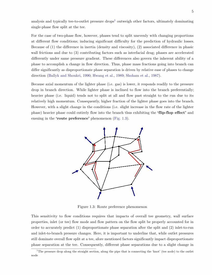
Because axial momentum of the lighter phase (i.e. gas) is lower, it responds readily to the pressure
drop in branch direction. While lighter phase is inclined to flow into the branch preferentially;
heavier phase (i.e. liquid) tends not to split at all and flow past straight to the run due to its
relatively high momentum. Consequently, higher fraction of the lighter phase goes into the branch.
However, with a slight change in the conditions (i.e. slight increase in the flow rate of the lighter
phase) heavier phase could entirely flow into the branch thus exhibiting the ‘flip-flop effect’ and
ensuing in the ‘route preference’ phenomenon (Fig. 1.3).
Figure 1.3: Route preference phenomenon
This sensitivity to flow conditions requires that impacts of overall tee geometry, wall surface
properties, inlet (or tee) flow mode and flow pattern on the flow split be properly accounted for in
order to accurately predict (1) disproportionate phase separation after the split and (2) inlet-to-run
and inlet-to-branch pressure changes. Here, it is important to underline that, while outlet pressures
still dominate overall flow split at a tee, afore mentioned factors significantly impact disproportionate
phase separation at the tee. Consequently, different phase separations due to a slight change in
1The pressure drop along the straight section, along the pipe that is connecting the ‘knot’ (tee node) to the outletnode
6
(any one of these) contributing factors can cause different inlet-to-run and inlet-to-branch pressure
drops at the tee, however outlet pressures remain the same.
The flip-flop effect attributed to the route preference of condensate in natural gas pipeline systems
is first reported by Oranje (1973) who studied uneven phase separation problem in natural gas lines.
Oranje (1973) concluded that the change in the direction of lighter phase (gas) entering the branch
induced a pressure drop inside the branch thus creating a suction force driving the secondary phase
(liquid) into the branch.
Later, Hong (1978) observed that as inlet gas flow rate increases (for a fixed liquid viscosity and
flow rate), the centripetal force acting on a unit mass of the liquid increases (perhaps associated
with a higher pressure drop). Consequently more liquid is drawn into the branch. While, for a
fixed gas flow rate, an increase in liquid rate raises the inertial force of the liquid without much
change in the centripetal force. Thus, less liquid tends to turn into branch. Also, an increase in the
liquid viscosity slows down the liquid, lowering axial momentum (inertial force) of the liquid phase;
thus, generally ensues in an increased branch liquid intake. Furthermore, Azzopardi and Whalley
(1982) reported that gas entering the branch drags the liquid film with it in the case of annular flow.
Hence, pressure drop and interfacial drag constitute the centripetal force acting on the fluid stream.
In other words, when branch gas intake is small, centripetal force acting on the liquid phase is also
small compared to the inertial force (the momentum in the inlet direction) of the liquid stream.
Therefore, liquid mostly flows straight through the T-junction directly into the run. When mass
fraction of the branch gas intake exceeds a threshold value (critical gas intake), liquid tends to enter
the branch preferentially.
It is well established with reference to the Bernoulli equation that, when single phase (also two-phase)
split takes place at a T-junction, flow continuing straight in the axial direction to the run experiences
a pressure rise (pressure spike) due to flow area expansion. On the other hand, a pressure drop
is typically experienced by the flow turning to the branch because the magnitude of associated
‘irreversible’ losses are usually greater than the Bernoulli type pressure rise due to flow expansion in
the branch.
Presence of recirculation zones (secondary flows) both in the run and branch, as well as the two-
dimensional nature of flow right after the split (at the T-junction), by default, demand that full
set of Navier-Stokes equations should be employed for multidimensional (i.e. 2D or 3D) analysis
and rigorous definition (and solution) of flow through T-junctions (Fig. 1.4). In fact, following the
incredible progress of computational power and modeling capabilities with Navier-Stokes equations,
two-fluid based multidimensional CFD is likely to become the de facto state-of-the-art for the
modeling of flow through T-junctions. Besides in-house two-dimensional Ellison et al., 1997;
Hatziavramidis et al., 1997 and three-dimensional Adechy and Issa, 2004; Issa and Oliveira, 1994,
flow split and phase separation problem has been studied with general purpose commercial CFD
software as well (Al-Wazzan, 2000; Lahey, 1990; Kalkach-Navarro et al., 1990). Typically, satisfactory
agreement with experimental observations is reported, at least in terms of capturing ‘broad features’
of the split. However, it has also been pointed out that certain details were not captured accurately
7
due to fact that particular phenomena is not represented inherently by the governing equation set
(Adechy and Issa, 2004).
Figure 1.4: Sample 3D computational grids for T-junctions (from Adechy and Issa, 2004; Lahey,1990)
Nevertheless, despite the enormous computational power of the day, modeling all the junctions of a
large, complex pipe network using 3D CFD is a computationally demanding task, and probably
not going to be a feasible approach in the near future for the purpose of modeling large networks.
Moreover, such degree of detail is seldom, if not at all, necessary for the purpose of modeling
network flow. Therefore, proper representation of two-phase flow split mechanism at junctions using
one-dimensional analysis is required.
An important aspect of modeling hydrocarbon condensate route preference in natural gas networks is
the inherent challenge of accounting for the compositional change of the stream. Overall composition
of delivered fluids could differ significantly from original composition after consecutive uneven phase
separations along the way to the delivery station.
Martinez and Adewumi (1997) developed a steady-state open network model by incorporating a
marching algorithm based two-phase flow model with Bernoulli equation based Double Stream
Model (DSM) of Hart et al. (1991) for T-junctions. Changes in stream composition after flow
split at junctions are accounted for using a so called ‘separator approach’ (cf. Sec. 4.13). DSM is
essentially a phase separation sub-model (see Secs. 3.2.1 and 3.2.3) for T-junctions and computes
outgoing phasic flow rates based on inlet conditions of the tee. In that regard, although a separate
model is employed at the tee, ‘forward’ workflow aspect of DSM is similar to marching algorithms
and works effectively in the analysis of open networks. In their study, Martinez and Adewumi (1997)
specified inlet pressures and all inlet/outlet gas flow rates as boundary conditions. Moreover, gas
phase split at each junction is either provided by the user or computed from already specified flow
rate data. The overall network solution has two parts; first, marching algorithm propagates the
solution from pipe inlet to a tee. Then, DSM determines the liquid flow rates to be prescribed as
inlet conditions for outgoing arms of the junction (in addition to specified gas rates). Afterwards,
again the marching algorithm advances the solution along the outgoing arms until a new tee or
a delivery station is reached. Consequently, approach is limited to the analysis of open networks.
Furthermore, in its original form, DSM is not completely adequate in addressing the route preference
phenomenon since flow split, in fact, depends on downstream conditions (pressures) as well.
8
Ottens et al. (2001) developed a finite-difference based transient T-junction model by combining
transient equations that relate pipe liquid level to phasic superficial velocities (derived from phasic
mass and momentum equations) with an advanced version of DSM.
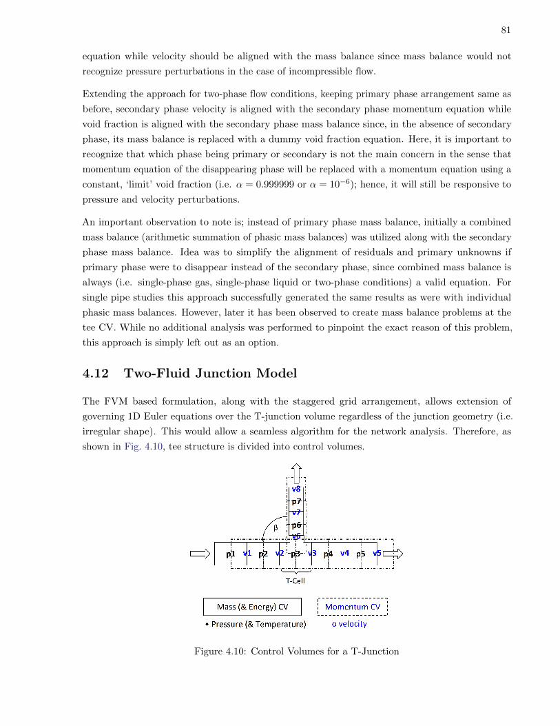
In a recent study, Singh (2009) developed a finite-volume based one-dimensional two-fluid model
(see Chapter 4) for steady-state analysis of isothermal air-water split at T-junctions. Benefiting from
the FVM staggered grid, Euler equations are easily extended over the T-junction control volume
(Spore et al., 2001). Nevertheless, study of Singh (2009) had two inherently contentious aspects: (1)
Over specification of boundary conditions – void fractions are specified at the outlets, in addition to
the pressures. This is attributed to a possible misconception regarding the calculation of two-phase
pressure gradient term in the two-fluid model momentum equations. Please see pertinent discussions
regarding the use of void fraction, or holdup for that matter, when writing phasic pressure gradient
terms for the derivation of phasic momentum equations both in PDE and algebraic forms (cf.
Sec. 4.3.2). (2) Direct substitution of Gardel2 mechanical energy loss coefficients (intended for use
with Bernoulli equations) as momentum correction factors in the phasic momentum equations (cf.
Secs. 3.2.3 and 4.12). Utilized loss coefficients inherently account for the branching angle effect
(which is not accounted for by the non-directional Bernoulli equations otherwise) while momentum
equations already accounted for the directional momentum change with an additional term involving
the branching angle.
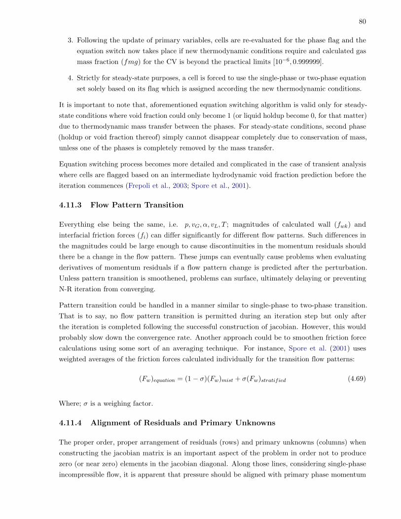
In this study, one-dimensional steady-state analysis of two-phase flow split at branching T-junctions
is formulated using the two-fluid model based integrated pipe approach. Governing Euler equations
are discretized over a staggered grid using the inherently conservative Finite Volume Method
(FVM, cf. Chapter 4). The staggered grid arrangement allows seamless extension of Euler equations
over the T-junction control volume and adjoining pipe flow equation set with the Double Stream
Model of Hart et al. (1991), essentially a phase separation sub-model, applied at the junction control
volume. In order to have a consistent model, phasic momentum equations of the tee CV are replaced
with gas phase Bernoulli equations at junction cell volume and required loss coefficients (K-factors)
are calculated using Gardel correlations (cf. Secs. 3.2.3). Focus is kept on the analysis of flow split at
horizontal, regular, 90o angle branching tee arrangements with single-phase, mist and stratified flow
patterns separately. Phases are assumed to be in thermodynamic equilibrium; implying mechanical,
thermal and chemical equilibrium between the phases. As a requirement of steady-state analysis
overall mixture composition remains constant along straight sections of the pipe system; i.e. along
each pipe and each arm of a T-junction. Interaction between the phases is represented by mass and
momentum transfer terms and interfacial friction terms. Due to thermal equilibrium assumption
an overall energy equation is utilized. Peng-Robinson EoS based thermodynamic model is used
for phase behavior predictions (Appendix C). Using a generalized Newton-Raphson technique,
numerical solution is obtained for all discrete points (control volumes) on all three arms of the
junction simultaneously, hence the name ‘integrated pipe’ approach. This approach proves to be
essential for closed-loop network analysis as it circumvents the need for marching through the flow
domain in one direction and readily accounts for changes in downstream conditions, particularly the
2Gardel, A. (1957). Les pertes de charge dans les ecoulements au travers de branchementes en te. BulletinTechnique de la Suisse Romande, 9,122 and 10, 143. (Ottens et al., 2001)
9
outlet pressures in this case.
In Chapter 2, solutions of single-phase steady-state flow in conduits and two-phase flow models are
introduced. In Chapter 3, flow split mechanism and uneven phase separation is discussed along
with a survey of available methods with emphasize on phenomenological and mechanistic junction
models. Appendix A presents conventional single-phase network analysis in oil and gas industry.
In Chapter 4, one-dimensional two-fluid model equations are derived based on FVM. Staggered
grid, boundary conditions, T-junction momentum equations and double stream model integration
is discussed along with the handling of phase appearance-disappearance. Appendix B has an
alternative derivation for a dividing streamline based ‘double channel’ T-junction model for FVM.
Chapter 5 includes results from numerical model comparison with single-phase steady-state analytical
solution, single-phase to two-phase transition handling in a single pipe and two-phase flow split
results for air-water and hydrocarbon two-phase flows through T-junctions.
10
Chapter 2
Flow In Conduits
Analysis of flow in conduits is fundamental to various engineering applications of different scales.
Evidently, quantitative description of flow and predicting response to perturbations (i.e. changes
in flow conditions) are essential for engineering designs. This requires determining the values of
governing flow parameters and fluid properties; such as flow rate or velocity, pressure, temperature
and fluid density. Study of flow in conduits is based on the principles of conservation of mass
(continuity), momentum, and energy. Several methods are available for the description of fluid flow
in pipes, with varying levels of detail, complexity and accuracy. Depending on the complexity of
the problem and level of detail desired for the analysis; an entire suite of conservation equations, or
a subset of them, is written along with appropriate simplifying assumptions in order to describe
the flow. It is then possible to quantify parameters governing the flow by solving the conservation
equations. Three-dimensional flow field is governed by Navier-Stokes equations; a comprehensive set
of coupled, nonlinear partial differential equations (PDEs) expressing conservation principles over
the flow domain; the continuum of conduit, and account for viscous and local volume (fluid particle)
forces. For the practical purposes of flow analysis in pipeline networks, where flow property changes
in the radial direction are not as important as property changes along the axial direction, one-
dimensional statements of mass, momentum, and energy conservation provide sufficient detail and
information on the flow. Typically, conservation statements can be generalized for one-dimensional
analysis through the following conservation differential form:
∂
∂t
[Conserved
property p.u.v.
]+
∂
∂x
[Flux of conserved
property p.u.v.
]=
External forcing function p.u.v.
(source/sink)(2.1)
Where; p.u.v. stands for ‘per unit volume’ and ‘flux of conserved property’ is defined as the amount
crossing the unit area, per unit time [(unit of conserved property) L−2 t−1].
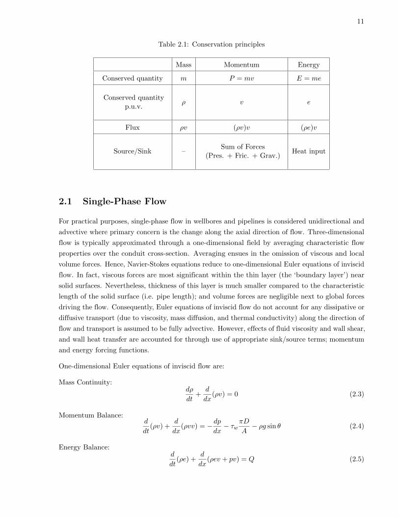
Table 2.1 illustrates the relationship among the three conservation principles; where, intrinsic
energy of fluid is sum of its internal, kinetic, and potential energy. It is the energy associated
with fluid at each point of the pipe and accounts for fluid’s internal energy stored at molecular
level (e∗) and additional energy associated due to its velocity (kinetic energy) and location in the
gravitational field (potential energy). Hence, intrinsic energy per unit mass of the working fluid is:
e = e∗ +v2
2+ g∆zel (2.2)
11
Table 2.1: Conservation principles
Mass Momentum Energy
Conserved quantity m P = mv E = me
Conserved quantityp.u.v.
ρ v e
Flux ρv (ρv)v (ρe)v
Source/Sink –Sum of Forces
(Pres. + Fric. + Grav.)Heat input
2.1 Single-Phase Flow
For practical purposes, single-phase flow in wellbores and pipelines is considered unidirectional and
advective where primary concern is the change along the axial direction of flow. Three-dimensional
flow is typically approximated through a one-dimensional field by averaging characteristic flow
properties over the conduit cross-section. Averaging ensues in the omission of viscous and local
volume forces. Hence, Navier-Stokes equations reduce to one-dimensional Euler equations of inviscid
flow. In fact, viscous forces are most significant within the thin layer (the ‘boundary layer’) near
solid surfaces. Nevertheless, thickness of this layer is much smaller compared to the characteristic
length of the solid surface (i.e. pipe length); and volume forces are negligible next to global forces
driving the flow. Consequently, Euler equations of inviscid flow do not account for any dissipative or
diffusive transport (due to viscosity, mass diffusion, and thermal conductivity) along the direction of
flow and transport is assumed to be fully advective. However, effects of fluid viscosity and wall shear,
and wall heat transfer are accounted for through use of appropriate sink/source terms; momentum
and energy forcing functions.
One-dimensional Euler equations of inviscid flow are:
Mass Continuity:dρ
dt+
d
dx(ρv) = 0 (2.3)
Momentum Balance:d
dt(ρv) +
d
dx(ρvv) = −dp
dx− τw
πD
A− ρg sin θ (2.4)
Energy Balance:d
dt(ρe) +
d
dx(ρev + pv) = Q (2.5)
12
Energy balance is usually written in terms of enthalpy flux for an open system:
d
dt(ρe) +
d
dx
(ρ
[h+
v2
2+ g∆zel
]v
)= Q (2.6)
Where;
h = e∗ +p
ρ(2.7)
Please note that no shaft work is considered for pipe flow. Also, no boundary work is present when
a control volume approach is adopted.
Euler equations could be solved analytically only in the limiting case where a perturbation in
the flow is assumed to occur instantaneously everywhere along the conduit (i.e. the rigid column
flow; Larock et al., 2000) or for steady-state conditions. For other flow conditions, Euler equations
must be solved simultaneously, which requires implementation of appropriate numerical schemes.
Numerical solutions provide approximate values of the flow parameters at discrete points in the
flow domain, which is generally sufficient for most practical purposes.
2.1.1 Single-Phase Steady-State Flow
It is customary to introduce simplifications in the conservation equations based on steady-state
assumptions and expected fluid phase behavior in the system. For steady-state conditions, the
governing equations simplify to:
Mass Continuity:d
dx(ρv) = 0 (2.8)
Momentum Balance:d
dx(ρv v) = −dp
dx− τw
πD
A− ρ g sin θ (2.9)
Energy Balance:d
dx
[ρ v
(e+
p
ρ
)]= cU
πD
A(T∞ − T ) (2.10)
Starting from steady-state momentum and mass balances, one obtains:
d
dx(ρv v) = ρ v
dv
dx+ v
0︷ ︸︸ ︷d
dx(ρ v) = −dp
dx− τw
πD
A− ρg sin θ (2.11)
From where following steady-state pressure gradient (pressure drop) equation is obtained:(dp
dx
)total
=
(dp
dx
)fric
+
(dp
dx
)elev
+
(dp
dx
)acc
(2.12)
13
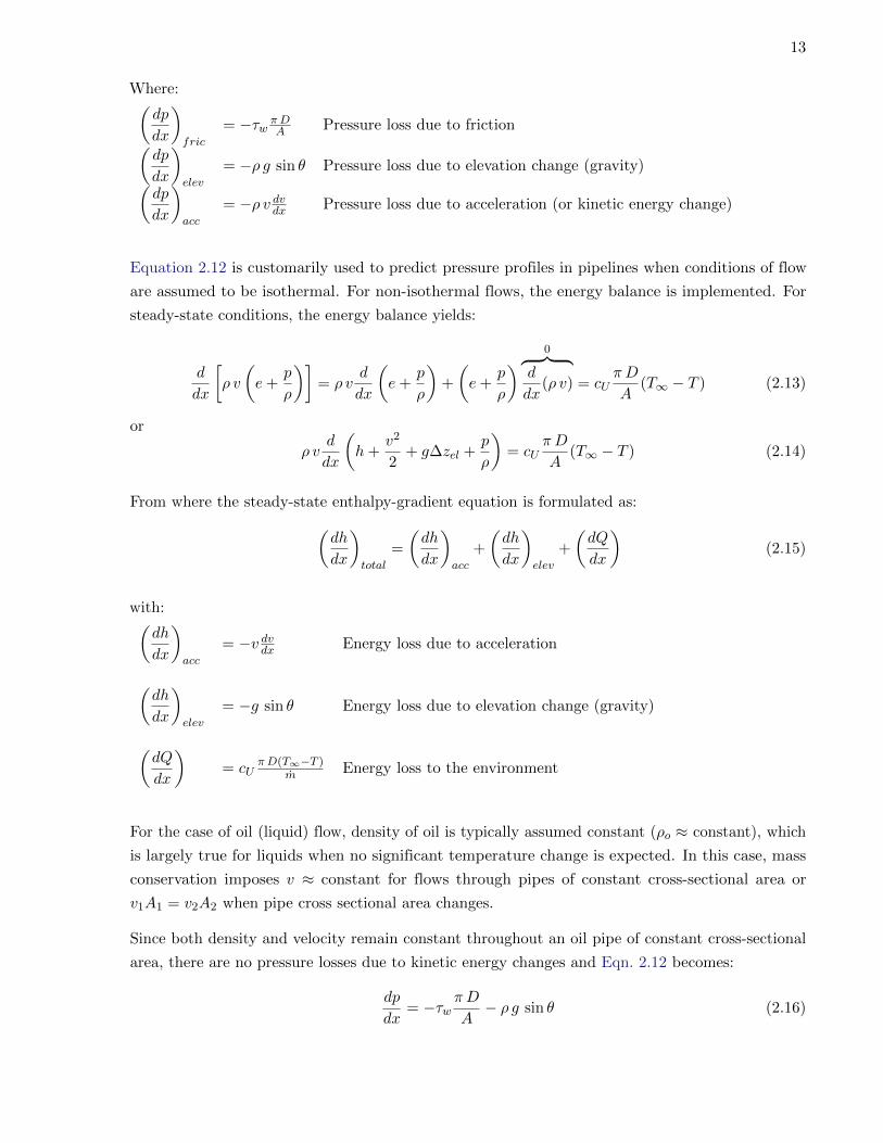
Where:(dp
dx
)fric
= −τw πDA Pressure loss due to friction(dp
dx
)elev
= −ρ g sin θ Pressure loss due to elevation change (gravity)(dp
dx
)acc
= −ρ v dvdx Pressure loss due to acceleration (or kinetic energy change)
Equation 2.12 is customarily used to predict pressure profiles in pipelines when conditions of flow
are assumed to be isothermal. For non-isothermal flows, the energy balance is implemented. For
steady-state conditions, the energy balance yields:
d
dx
[ρ v
(e+
p
ρ
)]= ρ v
d
dx
(e+
p
ρ
)+
(e+
p
ρ
) 0︷ ︸︸ ︷d
dx(ρ v) = cU
πD
A(T∞ − T ) (2.13)
or
ρ vd
dx
(h+
v2
2+ g∆zel +
p
ρ
)= cU
πD
A(T∞ − T ) (2.14)
From where the steady-state enthalpy-gradient equation is formulated as:(dh
dx
)total
=
(dh
dx
)acc
+
(dh
dx
)elev
+
(dQ
dx
)(2.15)
with:(dh
dx
)acc
= −v dvdx Energy loss due to acceleration
(dh
dx
)elev
= −g sin θ Energy loss due to elevation change (gravity)
(dQ
dx
)= cU
πD(T∞−T )m Energy loss to the environment
For the case of oil (liquid) flow, density of oil is typically assumed constant (ρo ≈ constant), which
is largely true for liquids when no significant temperature change is expected. In this case, mass
conservation imposes v ≈ constant for flows through pipes of constant cross-sectional area or
v1A1 = v2A2 when pipe cross sectional area changes.
Since both density and velocity remain constant throughout an oil pipe of constant cross-sectional
area, there are no pressure losses due to kinetic energy changes and Eqn. 2.12 becomes:
dp
dx= −τw
πD
A− ρ g sin θ (2.16)
14
which, when integrated between two points separated by a distance L, becomes:
(pout − pin) = −πf8
q2LρLD5
L− ρLg∆z (2.17)
Or, re-arranged as:
qL =
√8
π
√1
f
√pin − pout + ρLg∆z
ρLLD
52 (2.18)
Where:
f = 4τw2
ρv2Darcy-Weisbach friction factor and f = 4fFanning
Equations 2.17 and 2.18 are typical pressure-loss and flow rate equations used for liquid-system
calculations. When the definition of friction factor for laminar flow conditions (f = 64/Re) is
substituted, the Poiseuille’s equation for laminar liquid flow through a pipe of uniform (circular)
cross-section is obtained.
For the case of natural gas (compressible) flow, fluid density is a strong function of pressure and
temperature. However, it is still customary to neglect contribution of kinetic energy change in the
pressure gradient equation for gas flow because kinetic energy change contribution is typically very
small compared to the friction and elevation terms; hence, one ends up with the Eqn. 2.16 again.
When pressure-gradient equation for gas flow is integrated between two points separated by a
distance L, the density dependency with pressure is accounted for by means of the real gas law
equation. For isothermal flow conditions, this integration yields a stronger dependency of flow rate
on pressure; i.e. squared pressures (Kumar, 1987):
qG = C
(Tscpsc
)√1
f
√p2in − p2
out es
γGTavgZavgLeD
52 (2.19)
Where:
s =2MWair γG ∆z
1000TavgZavgR
g
gcPipe inclination dependent coefficient, s = 0 for horizontal pipe
[dimensionless]
Le = Les − 1
sThe ‘equivalent’ length definition based on s [m]
C =
√1000 gcπ2R
16MWairA unit system dependent constant [m2s−2K−1]
e The base of natural logarithm [≈ 2.718282]
γG Gas gravity (or gas specific gravity) [dimensionless]
15
On the basis of Eqn. 2.19, several gas flow equations have been proposed throughout the years.
Steady-state empirical gas flow equations such as Spitzglass, Weymouth, Panhandle-A, Panhandle-B,
and the IGT/AGA differ in the functional form simply because each equation utilizes a different
expression for the calculation of friction factor in Eqn. 2.19.
The analytical expressions derived above (Eqn. 2.18 and 2.19) allow calculation of pipe pressure
drops for isothermal, single-phase flow systems. However, flow of liquid and gases may not be
well represented by an isothermal model, especially when fluid inlet temperature greatly differs
from ambient temperature, which creates non-adiabatic conditions throughout the length of the
pipe. Even during adiabatic conditions, natural gas pipelines tend to cool with distance (the‘Joule-
Thomson cooling’ effect), while oil lines tend to heat – because of the very distinct Joule-Thomson
coefficient values of liquids and gases. Therefore, for non-isothermal, steady-state, single-phase flow,
the enthalpy-gradient equation is implemented:(dh
dx
)total
=
(dh
dx
)acc
+
(dh
dx
)elev
+
(dQ
dx
)(2.20)
which, integrated between two points in the pipeline separated a distance x, yields the following
explicit expression for the calculation of temperature change as a function of pressure drop:
T (x) = T∞ + (T0 − T∞)e−φ1x + (1− e−φ1x)
(η
φ1
dp
dx− φ2
φ1
)(2.21)
Where:
T0 Fluid temperature at the pipe inlet [K]
T∞ Surrounding (ambient) temperature [K]
φ1 =cUcp
πD
mHeat transfer factor [m−1]
φ2 =v
cp
dv
dx+g
cp
dzeldx
Potential and kinetic energy factor [Km−1]
Equation 2.21 gives the explicit dependency of temperature on (1) pressure drop (dp/dx), (2) heat
transfer from the environment (φ1), and (3) potential and kinetic changes (φ2). When last two
factors two are neglected, Eqn. 2.21 collapses to the following equation (Coulter, 1979):
T (x) = T∞ + (T0 − T∞)e−φ1x + (1− e−φ1x)η
φ1
dp
dx(2.22)
When one further assumes that thermodynamic changes on fluid pressure do not affect the tempera-
ture of the fluid (i.e. Joule-Thomson coefficient is close to zero); Eqn. 2.22 can be further simplified
to:
ln
(T (x)− T∞T0 − T∞
)= −φ1x (2.23)
Equation 2.23 neglects the changes in fluid enthalpy due to pressure, which can be a reasonable
assumption for liquids. For the derivation of Eqn. 2.23, fluid’s enthalpy changes are implicitly
16
evaluated through the simplified expression dh = cpdT instead of the more rigorous dh = cpdT −ηcpdp.
For simultaneous prediction of pressure and temperature changes along a pipeline, one may resort
to using an analytical flow equation for dp/dx calculations and the analytical energy equation for
dT/dx calculations, working concurrently. However, such approach decouples the combined effect
that pressure and temperature changes can have on fluid density. This might be acceptable for oil
or liquid flows but not for natural gas flows.
2.2 Two-Phase Flow
Two-phase flow occurs during production and transportation of oil and gas, where formation of
the condensed liquid (hydrocarbon or water) is determined by the overall mixture composition and
local P-T couple, according to thermodynamic phase behavior.
In order to adequately describe two-phase flow, new variables need to be defined in addition to the
fundamental single-phase flow parameters pressure, velocity and temperature:
Holdup is the liquid phase volume fraction within a volume element.
αL =VL
VL + VG=ALA
(2.24)
Void fraction, on the other hand, is the gas phase volume fraction in a given volume element.
αG =VG
VL + VG=AGA6= qGqL + qG
(2.25)
In that regard, these two parameters are the analogs of liquid and gas phase saturations in reservoir
engineering.
αL + αG = 1 (2.26)
Phasic superficial velocity is defined as the ratio of phasic volumetric flow rate to the whole
conduit cross-sectional area.
uk =qkA
(2.27)
Phasic velocity (intrinsic) is the ratio of phasic volumetric flow rate to the cross-sectional area
available for the phase in conduit.
vk =ukαk
(2.28)
Mixture velocity is the total volumetric flow rate of both phases per unit area.
vmix =qG + qLA
(2.29)
17
Slip velocity is the velocity of gas phase relative to liquid phase.
vslip = vG − vL (2.30)
Drift velocity, however, is the velocity of each phase relative to mixture velocity.
(vk)drift = vk − vmix (2.31)
Drift flux is the per unit area flow rate of each phase, relative to mixture velocity.
Jk = αk(vk − vmix) (2.32)
Phasic volume fraction is distinguished from holdup or void fraction as the ratio of phasic
superficial velocity to the mixture (sum of phasic) superficial velocities.
Λk =ukumix
=uk
uG + uL=
qGqL + qG
(2.33)
Please note that holdup (or void fraction) is equal to phasic volume fraction (αk = Λk) only for
no-slip condition (i.e. vG = vL).
Quality is the ratio of gas mass flow rate to the total mass flow rate.
x =mG
mG + mL=mG
m(2.34)
2.2.1 Flow Patterns
Gas-liquid two-phase flows are typically categorized according to the governing ‘flow pattern’;
distinct geometric arrangements of phasic volumes, the structure and continuity of the phasic
interface in the conduit. Various flow patterns (Fig. 2.1) fall under three major flow types (Shoham,
2006):
1. Dispersed flows: Bubbly (gas bubbles) or mist (liquid droplets) flow patterns, where particle
size secondary phase is ‘dispersed’ in the continuous phase.
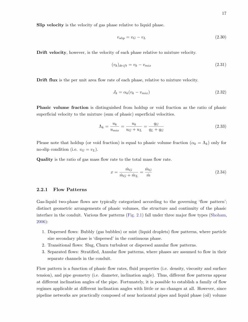
Ideally, a T-junction model should be consistent and complete in capability; predicting inlet-
to-run and inlet-to-branch pressure changes as well as uneven phase separation at a tee with
reasonable accuracy and consistency. Therefore, there are two components, called ‘sub-models’,
to a T-junction model, that determine overall success and prediction capabilities:
1. Pressure change sub-model
2. Phase separation sub-model
Sub-models are usually tested by substituting experimental data. For instance, experimental phase
distribution data is substituted in the governing equations of pressure change component to match
pressure change information that is typically obtained through extrapolation of observed pressure
profiles for developed flow along the run and branch, thus establishing the pressure change component.
Similarly, pressure change data (often extrapolated from developed flow profiles) is substituted
30
in the governing equations for phase separation component in order to match experimental phase
separation data. However, extrapolation of pressure profiles in order to obtain pressure change data
and separately substituting experimental data in sub-models has the potential danger of leading
to a weak coupling between two components of the model, rendering seemingly separate ‘pressure
change’ and ‘phase separation’ models. Consequently, individual success of sub-models does not
necessarily guarantee consistency for the overall model.
One-dimensional modeling efforts for the analysis of two-phase flow split at T-junctions fall under
three categories (Azzopardi, 1999; Peng and Shoukri, 1997; Lahey, 1986):
1. Empirical correlations; i.e. phase separation sub-model of Seeger et al. (1986).
2. Phenomenological and Mechanistic1 models; i.e. Penmatcha et al. (1996); Ballyk and Shoukri
(1990). Following the discussion of Lahey (1986), approaches such as fluid mechanics based
(hence ‘mechanistic’) models of Penmatcha et al. (1996); Saba and Lahey (1984); Fouda and
Rhodes (1974), are considered under this category.
3. Two-fluid models (control volume based); i.e. TRAC family of thermal-hydraulic codes
(Spore et al., 2001; Steinke, 1996). Although Peng and Shoukri (1997) classifies only two and
three-dimensional models as two-fluid models (i.e. Adechy and Issa, 2004; Ellison et al., 1997),
TRAC extends one-dimensional2 two-fluid model approach over the tee control volume.
Empirical correlations represent the two-phase flow split in a much simplified way that usually
leads to analytical solutions. For instance, Seeger et al. (1986) developed correlations for phase
separation at T-junctions with different branch inclinations. Unfortunately, empirical correlations
are usually valid only in the range of conditions from which they are derived. Besides, accuracy
of predictions typically depends on the amount and quality of experimental data utilized in the
derivation of correlations.
Phenomenological–mechanistic models, on the other hand, represent complicated physics of
flow separation using conservation principles (mass, momentum and/or mechanical energy) and force
balances (i.e. inertial vs. centripetal force balance on fluid particles based on streamline geometry)
that are simplified with assumptions according to physical understanding of the split mechanism. The
simplifications generally lead to models with analytical solutions. Particularly, phenomenological
methods are usually junction type (i.e. diverging, merging or impacting), geometry, and flow
pattern dependent. Also, closure relations or certain parameters such as energy loss coefficients or
momentum correction factors are expected to involve empirical correlations of such dependence.
However, applicability of phenomenological–mechanistic models can be usually extended to wider
range of flow conditions, extrapolated well outside the range on which the model is based.
An intriguing approach is the conformal mapping technique applied to two-phase flow split by
Hatziavramidis et al. (1997). Originally suited for two-phase flows that can be approximated as
potential flow (i.e. irrotational flow of incompressible and inviscid fluids), the model also employs
1Mechanistic T-junction models not to be confused with mechanistic two-phase flow modeling approach2Even for one-dimensional analysis, flow split at a branching tee requires at least two dimensions to be accounted
for; in the directions of (1) run and (2) branch, hence the term ‘one-half’ dimensional (1.5D) model.
31
the concept of the ‘free streamline’ (dividing streamline), defining the boundary of flow split at the
tee (Fig. 3.5).
One-dimensional Two-fluid models are based on the solution of one-dimensional mass and
momentum conservation equations for both phases, in both directions. In essence, two-fluid junction
model is the extension of two-fluid flow model over the junction control volume. As discussed earlier
in Sec. 2.2.2, two-fluid flow model is a rigorous approach for modeling two-phase flow in conduits,
giving rise to the simultaneous solution of coupled conservation equations (mass and momentum
balances) for phases. In fact, what separates two-fluid junction models from mechanistic junction
models is the use of phasic momentum equations in both run and branch directions (hence an
additional, 6th momentum equation) by the two-fluid models (cf. Sec. 4.12).
Success of two-fluid based junction models depends on the description of ‘irreversible’ flow loss
terms; in particular, availability of correlations for appropriate momentum correction k-factors.
Derivation of one-dimensional two-fluid model junction equations are discussed in more detail in
Sec. 4.12
A ‘complete phase separation’ is achieved at ‘critical branch flow split ratio’, when all
of the incoming gas phase is completely extracted through the branch. When complete phase
separation occurs, the T-junction indeed becomes a functional two-phase separator:
λcritical =m3
m1=x1
x3(3.3)
or
m3x3 = m1x1 (3.4)
3.2 Phenomenological and Mechanistic Junction Models
For one-dimensional analysis of steady-state, isothermal two-phase flow through a branching tee,
and assuming that junction geometry (arm inclination and diameters, branching angle, geometry of
joint corners etc.) and wall surface properties (pipe roughness) are known, there are 9 parameters
of primary interest that adequately define (and quantify) flow through the junction, hence the split:
• phasic mass flow rates through each arm (= 2× 3 = 6)
• inlet, run and branch pressures (= 3)
A 10th parameter of particular interest would have been a representative, nodal pressure for the tee.
However, modeling (at least) a two-dimensional pressure distribution with a single pressure node is
a significant challenge (cf. Sec. 4.12 and Appendix B).
For a well posed problem, that is for a unique solution to exist without over specifying the problem,
4 out of 9 parameters can be specified. Then, 5 linearly independent equations are required to
account for remaining 5 unknown parameters.
32
Conventionally, inlet phasic mass flow rates (2) and either run or branch phasic mass flow rates (2),
thus a total of 4 parameters are specified for the analytic solution. In Sec. 4.12 where two-fluid model
based flow split is discussed using a staggered grid arrangement for numerical solution, inlet phasic
mass flow rates and both run and branch outlet pressures are specified as boundary conditions.
Typically, four equations are employed by default when constructing phenomenological–mechanistic
models:
1. mixture mass balance for the tee
2. gas phase mass balance for the tee
3. inlet-to-run mixture momentum balance (or mechanical energy balance)
4. inlet-to-branch mixture mechanical energy balance (or momentum balance)
Mixture (or overall) momentum or mechanical energy balance equations, simplified into inlet-to-run
and inlet-to-branch pressure change equations, indeed constitute the pressure change component of
the model.
A 5th relation, required for completing the equation set, constitutes the phase separation component
of the model determining the degree of separation. In fact, the essential difference between several
T-junction models and what renders them phenomenological or mechanistic is the choice of this 5th
relation and associated constitutive (closure) relations for the calculation of certain parameters (i.e.
two-phase loss multiplier in pressure change equations of homogeneous equilibrium based models
and etc.).
By nature, phenomenological models are expected to be flow pattern dependent. On the other
hand, mechanistic junction models are thought to be flow pattern independent. However, employed
closure relations are frequently flow pattern dependent. Typically, flow pattern specific models
are expected to perform better than independent models. Lahey (1986) provides a list of most
significant branching T-junction studies of the time, categorizing the studies according to analyzed
tee geometry and developed model; i.e. pressure change and/or phase separation model.
3.2.1 Pressure Change Sub-Models
Inlet-to-run and inlet-to-branch pressure changes dominating the flow split and phase separation at
a tee can be calculated using:
1. mechanical energy balances in both directions
2. momentum balances in both directions
3. mechanical energy balance for branch and momentum balance for run direction.
It is well established that (i.e. by reference to Bernoulli equation) when single or two-phase flow
split takes place at a T-junction, flow continuing in the inlet direction through the run experiences
a pressure rise due to deceleration associated with flow area expansion, assuming that main pipe
diameter does not change. On the other hand, typically a pressure drop is experienced by the flow
turning into the branch.
33
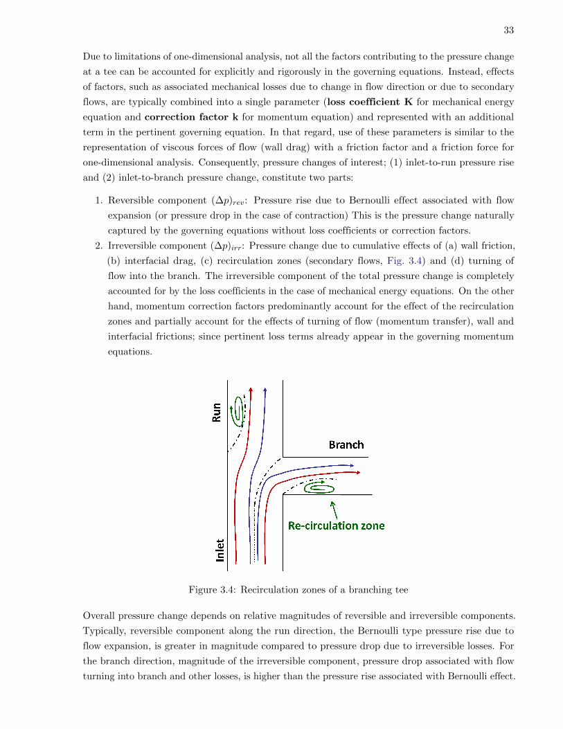
Due to limitations of one-dimensional analysis, not all the factors contributing to the pressure change
at a tee can be accounted for explicitly and rigorously in the governing equations. Instead, effects
of factors, such as associated mechanical losses due to change in flow direction or due to secondary
flows, are typically combined into a single parameter (loss coefficient K for mechanical energy
equation and correction factor k for momentum equation) and represented with an additional
term in the pertinent governing equation. In that regard, use of these parameters is similar to the
representation of viscous forces of flow (wall drag) with a friction factor and a friction force for
Where, Ck is the orifice discharge coefficient [dimensionless]
Saba and Lahey (1984) suggest a fluid mechanics based 5th equation to account for phase separation.
However, instead of a control volume based field equation (i.e. momentum or mechanical energy
equation) as in two-fluid models, inlet-to-branch gas phase momentum equation is integrated along
a ‘mean’ (approximate/average) streamline to yield an auxiliary relation for inlet-to-branch pressure
change from which phase separation is determined. The length Ls of the mean streamline is
calculated based on empirical correlations. Gas phase momentum equation is chosen over liquid
phase because gas phase was observed to determine the preferential separation as the ability of gas
to make the turn into branch is the dominant factor.
37
Phenomenological models are typically developed for annular flow pattern in the inlet and
geometrically define proportions of gas and liquid flows extracted from main line into the branch.
There are two fundamental concepts in model development:
1. zones of influence; sections of main line cross-sectional area from which liquid and gas are
diverted into the branch (Fig. 3.6).
2. dividing streamlines that separate incoming (inlet) flow into inlet-to-run and inlet-to-branch
streams for each phase (Fig. 3.5).
Inlet-to-branch streamlines of both phases follow curved paths in order to accomplish a turn into
the branch and typically, phasic streamlines are expected to cross if both phases are to make turn
in the branch direction.
Figure 3.5: Dividing streamlines for two-phase flow in a branching tee
Dividing stream line approach requires geometric analysis of inlet flow pattern to determine ‘zones
of influence’ that affect the outcome of force balance between gas and liquid phases over the
streamline(s) curving into the branch; i.e. competing inertial and centripetal forces. Distance of
streamlines from inlet pipe wall determine zones of influence.
Identifying zones of influence for phases is a semi-empirical step. ‘Zones’, geometric portions of
inlet gas and liquid flows, from which phases extracted to enter the branch are determined by
superimposing cross-sectional phase distribution of the inlet on dividing streamlines. A zone of
influence exists for each phase and dividing streamlines determine both the zone boundary and
phasic (Gas–liquid) interface in the main line. The amount of gas phase extracted to the branch
comes from the area bounded by gas phase dividing streamline and the liquid film boundary.
The concept of ‘zones of influence’ was extended to two-phase flow by Azzopardi and Whalley (1982)
aiming to describe liquid film and gas extraction from the main line for annular flow at a vertical
tee. Based on geometrical considerations only, the ‘zone of influence’ is defined by the angle σ
38
(a) Single-zone model (b) Two-zone model (c) Advanced two-zone model
Figure 3.6: Zones of influence for two-phase flow in a branching tee
covering the sector of material extraction, the liquid film arc of inlet cross-section (Fig. 3.6). The
model constitutes an alternative 5th equation derived from geometrical relations provided by ‘zone
of influence’ concept.
Azzopardi and Whalley (1982) model assumes liquid and gas are extracted from the same zone of
influence. This suggests coincidental dividing streamlines for liquid and gas phases. However, due
to the significant difference in axial momentum fluxes of two phases, the gas and liquid are expected
to have different dividing streamlines.
Recognizing short comings of the single zone of influence used by Azzopardi and Whalley (1982)
and purely geometric approach lead to its definition, Shoham et al. (1987) defined separate zones of
influence for phases, for the analysis of stratified and annular flows. Consequently, phasic zones of
influence are delineated by separate gas and liquid dividing streamlines. Position of liquid streamline
(i.e. distance from pipe wall) is determined by a simplified force balance for competing centripetal
and inertial forces acting on the liquid film, thus establishing the 5th equation for phase separation
component.
Hwang et al. (1988) combined Saba and Lahey (1984) model with zone of influence concept, again
defining a separate zone of influence per phase. Phase separation (gas flow into the branch) is
governed by force balance equations written per phase and derived from a ‘modified version’ of
Euler’s equation of motion (momentum equation for a particle traveling along a streamline). In this
case, an empirical correlation is utilized to determine phasic ‘mean’ streamlines as opposed to the
force balance employed by Shoham et al. (1987). While not lumped into a single equation, whole
phase separation sub-model itself substitutes for the ‘5th equation’ needed for closure.
Both Shoham et al. (1987) and Hwang et al. (1988) models assume that radial (horizontal) distance
of dividing streamlines from pipe wall, defined by (δL, δG) remain constant and independent of
vertical position on the plane of cross-section, in accordance with the original intent of vertical
39
annular flow analysis. However, the major difference between the models is how the positions of
streamlines is determined.
In an attempt to improve the performance of dividing streamlines approach of Hwang et al. (1988)
for annular flow in horizontal, equal-diameter T-junctions, Ballyk and Shoukri (1990) computes
the position of dividing streamlines at varied elevations of the inlet cross-section, introducing the
concept of ‘development length’.
Hart et al. (1991) with Double Stream Model (DSM), and then Ottens et al. (1994)3with Advanced
Double Stream Model (ADSM) further developed the concept of dividing streamlines for separated
flow patterns (i.e. stratified flow) using a purely fluid mechanics based approach. Both models
derive a governing equation for phase separation based on phasic Bernoulli (mechanical energy)
equations and associated loss coefficients. More detailed discussion on Double Stream Model follows
in Sec. 3.2.3.
Peng and Shoukri (1997) further developed and generalized the model of Ballyk and Shoukri (1990)
to account for the effect of gravity, hence branch inclination, on phase separation.
Penmatcha et al. (1996) combined the Hwang et al. (1988) and Shoham et al. (1987) models for
stratified wavy conditions. Separate momentum equations are written for phasic streamlines and
flow areas required for the equations are determined by inlet flow geometry. Marti and Shoham
(1997) extended this model for reduced T-junctions with different branch arm inclinations.
3.2.3 The Double Stream Model
Hart et al. (1991) developed Bernoulli equation based Double Stream Model (DSM) to predict flow
split at T-junctions based on the dividing (separating) streamline concept which assumes phases
flow along their individual channels or streamlines. DSM is essentially a phase separation sub-model
for separated flows. Although Bernoulli equation comes with the inherent simplifying assumption of
constant phasic density all throughout the T-junction volume, it is a reasonable assumption for an
adequately small tee volume.
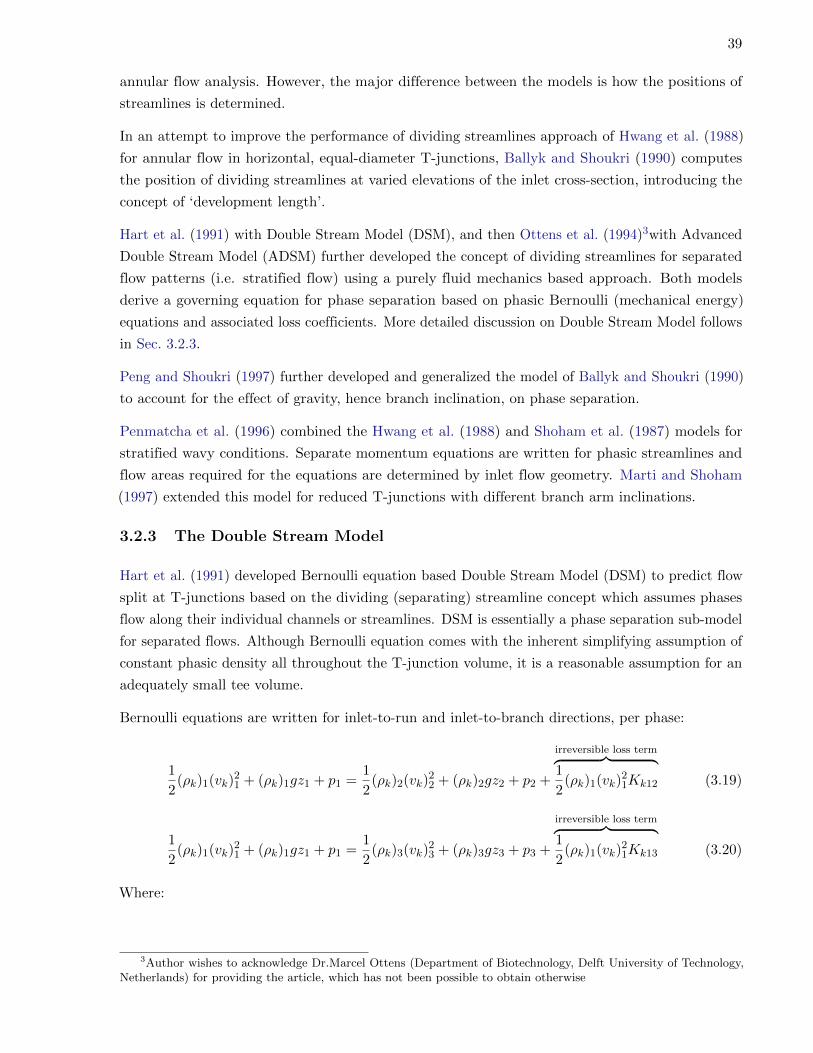
Bernoulli equations are written for inlet-to-run and inlet-to-branch directions, per phase:
1
2(ρk)1(vk)
21 + (ρk)1gz1 + p1 =
1
2(ρk)2(vk)
22 + (ρk)2gz2 + p2 +
irreversible loss term︷ ︸︸ ︷1
2(ρk)1(vk)
21Kk12 (3.19)
1
2(ρk)1(vk)
21 + (ρk)1gz1 + p1 =
1
2(ρk)3(vk)
23 + (ρk)3gz3 + p3 +
irreversible loss term︷ ︸︸ ︷1
2(ρk)1(vk)
21Kk13 (3.20)
Where:
3Author wishes to acknowledge Dr.Marcel Ottens (Department of Biotechnology, Delft University of Technology,Netherlands) for providing the article, which has not been possible to obtain otherwise
40
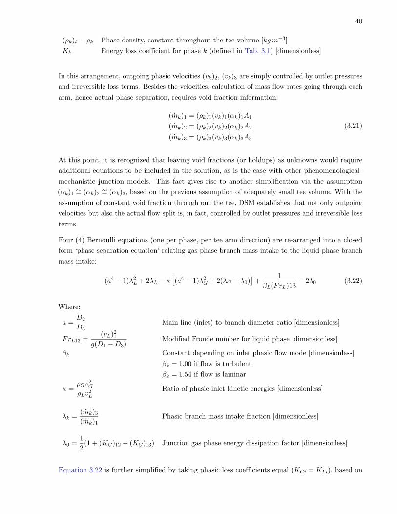
(ρk)i = ρk Phase density, constant throughout the tee volume [kgm−3]
Kk Energy loss coefficient for phase k (defined in Tab. 3.1) [dimensionless]
In this arrangement, outgoing phasic velocities (vk)2, (vk)3 are simply controlled by outlet pressures
and irreversible loss terms. Besides the velocities, calculation of mass flow rates going through each
arm, hence actual phase separation, requires void fraction information:
(mk)1 = (ρk)1(vk)1(αk)1A1
(mk)2 = (ρk)2(vk)2(αk)2A2
(mk)3 = (ρk)3(vk)3(αk)3A3
(3.21)
At this point, it is recognized that leaving void fractions (or holdups) as unknowns would require
additional equations to be included in the solution, as is the case with other phenomenological–
mechanistic junction models. This fact gives rise to another simplification via the assumption
(αk)1∼= (αk)2
∼= (αk)3, based on the previous assumption of adequately small tee volume. With the
assumption of constant void fraction through out the tee, DSM establishes that not only outgoing
velocities but also the actual flow split is, in fact, controlled by outlet pressures and irreversible loss
terms.
Four (4) Bernoulli equations (one per phase, per tee arm direction) are re-arranged into a closed
form ‘phase separation equation’ relating gas phase branch mass intake to the liquid phase branch
mass intake:
(a4 − 1)λ2L + 2λL − κ
[(a4 − 1)λ2
G + 2(λG − λ0)]
+1
βL(FrL)13− 2λ0 (3.22)
Where:
a =D2
D3Main line (inlet) to branch diameter ratio [dimensionless]
FrL13 =(vL)2
1
g(D1 −D3)Modified Froude number for liquid phase [dimensionless]
βk Constant depending on inlet phasic flow mode [dimensionless]
βk = 1.00 if flow is turbulent
βk = 1.54 if flow is laminar
κ =ρGv
2G
ρLv2L
Ratio of phasic inlet kinetic energies [dimensionless]
λk =(mk)3
(mk)1Phasic branch mass intake fraction [dimensionless]
λ0 =1
2(1 + (KG)12 − (KG)13) Junction gas phase energy dissipation factor [dimensionless]
Equation 3.22 is further simplified by taking phasic loss coefficients equal (KGi = KLi), based on
41
the assumption that phases are flowing along their separate streamlines (or channels). Nevertheless,
with this assumption DSM became limited to very small holdup values (αL ≤ 0.06) for accurate
phase separation predictions.
The most important point is, because it is based on mechanical energy equations, model had no
true way of recognizing the effect of split angle unless accounted for by other means; in this case by
the irreversible loss terms (and associated loss coefficients). Although Bernoulli equation is applied
on a streamline that curves into the branch, inherently the equation has no means of observing the
directional change in flow. This is to be expected since Bernoulli equation is indeed a non-vectorial
mechanical energy equation derived from a directional momentum balance with certain simplifying
assumptions Please see Munson et al. (2009) for the details of Bernoulli equation derivation from
momentum balance.
To make it more clear, without irreversible loss terms, Bernoulli equation can not account for a
directional change in flow (at least in its usual form and perception) and therefore DSM can not
account for the effect of split angle when irreversible losses are ignored. In a way, Steinke (1996)
also points out to this misconception lead by inadvertent approximation of split angle effects via
irreversible loss terms. However, Steinke (1996) discussion, or Spore et al. (2001) for that matter,
is quite interesting that Bernoulli equation is arranged in a form to resemble a non-conservative
momentum balance accounting for flow direction.
K-factors (loss coefficients) typically depend solely on surface properties (roughness) and geometry
of the conduit. The geometry element is expected to inherently introduce the effect of split angle.
Nevertheless, there is no certainty that a K-factor obtained by matching experimental data for
particular flow conditions, for a particular flow pattern and tee structure, would yield satisfactory
results for significantly different flow conditions and flow pattern if actual physics of the flow is not
properly acknowledged.
Ottens et al. (1994) relieved DSM from the small holdup constraint by deriving appropriate
correlations for liquid phase K-factors (KL) and establishing the Advanced Double Stream Model
(ADSM).
The advantage of DSM (or ADSM thereof), is, while it is certainly necessary to account for the
details of mechanisms controlling the split (i.e. flow pattern geometry), macroscopic balances should
be satisfied at all times and thus a satisfactory model employing simple energy or momentum
balances is preferable to flow pattern dependent methods. Nevertheless, when flow pattern geometry
and fluid distribution in the main line is not accounted for, DSM and similar mechanistic models
are likely to fail if branch diameter is smaller than main line diameter and/or side port orientation
is not horizontal (position of the opening for branch on the main line surface, not the inclination of
branch arm). Especially, if model has no way of recognizing liquid level or elevation of the highest
point the liquid film within the main line reaches it could still predict liquid phase going into the
branch while it is not physically possible. One-dimensional two-fluids model are also subject to
same problem unless a means to account for flow geometry is incorporated in the model.
42
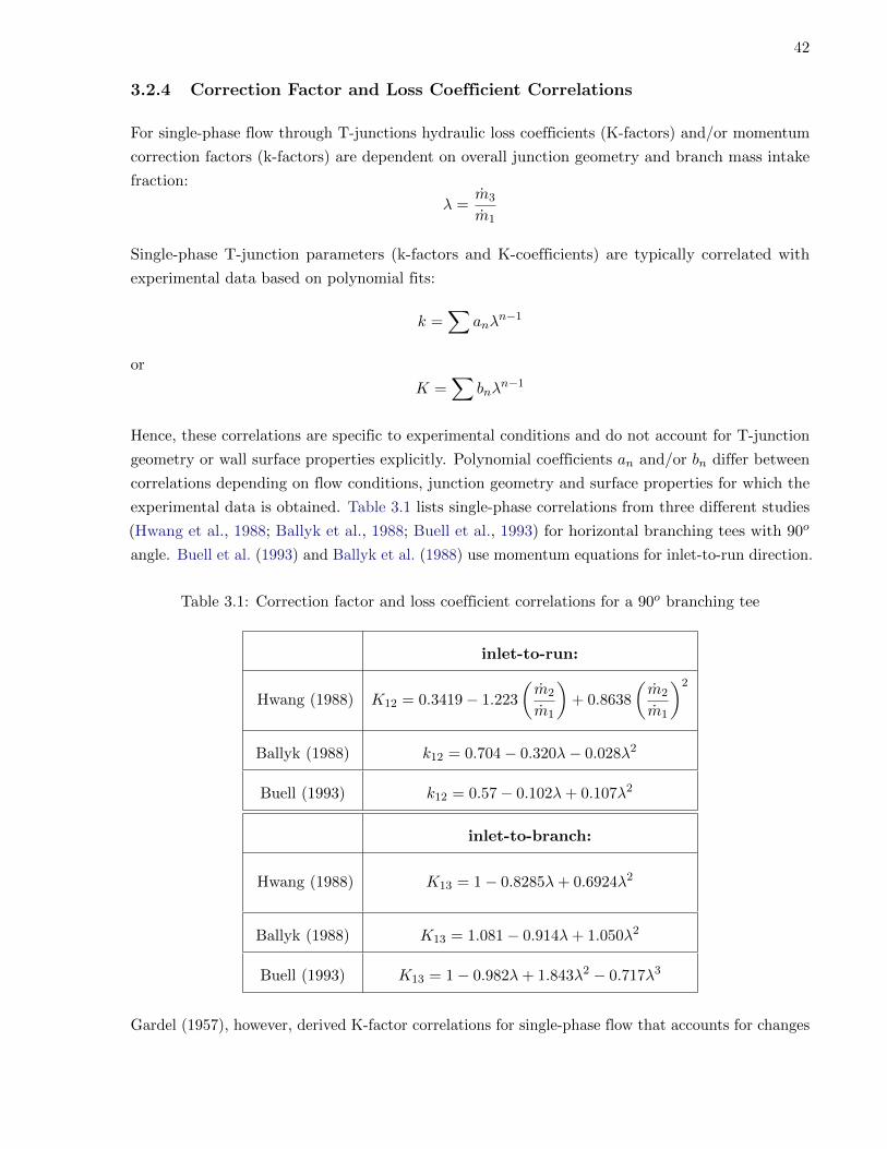
3.2.4 Correction Factor and Loss Coefficient Correlations
For single-phase flow through T-junctions hydraulic loss coefficients (K-factors) and/or momentum
correction factors (k-factors) are dependent on overall junction geometry and branch mass intake
fraction:
λ =m3
m1
Single-phase T-junction parameters (k-factors and K-coefficients) are typically correlated with
experimental data based on polynomial fits:
k =∑
anλn−1
or
K =∑
bnλn−1
Hence, these correlations are specific to experimental conditions and do not account for T-junction
geometry or wall surface properties explicitly. Polynomial coefficients an and/or bn differ between
correlations depending on flow conditions, junction geometry and surface properties for which the
experimental data is obtained. Table 3.1 lists single-phase correlations from three different studies
(Hwang et al., 1988; Ballyk et al., 1988; Buell et al., 1993) for horizontal branching tees with 90o
angle. Buell et al. (1993) and Ballyk et al. (1988) use momentum equations for inlet-to-run direction.
Table 3.1: Correction factor and loss coefficient correlations for a 90o branching tee
inlet-to-run:
Hwang (1988) K12 = 0.3419− 1.223
(m2
m1
)+ 0.8638
(m2
m1
)2
Ballyk (1988) k12 = 0.704− 0.320λ− 0.028λ2
Buell (1993) k12 = 0.57− 0.102λ+ 0.107λ2
inlet-to-branch:
Hwang (1988) K13 = 1− 0.8285λ+ 0.6924λ2
Ballyk (1988) K13 = 1.081− 0.914λ+ 1.050λ2
Buell (1993) K13 = 1− 0.982λ+ 1.843λ2 − 0.717λ3
Gardel (1957), however, derived K-factor correlations for single-phase flow that accounts for changes
43
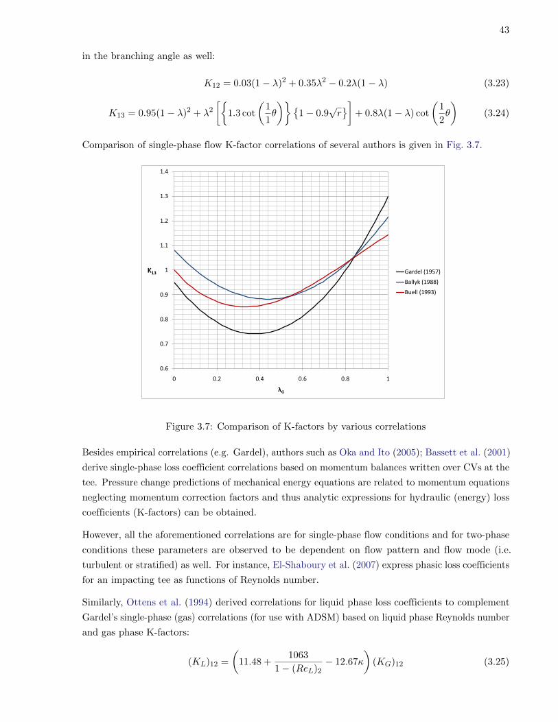
in the branching angle as well:
K12 = 0.03(1− λ)2 + 0.35λ2 − 0.2λ(1− λ) (3.23)
K13 = 0.95(1− λ)2 + λ2
[1.3 cot
(1
1θ
)1− 0.9
√r]
+ 0.8λ(1− λ) cot
(1
2θ
)(3.24)
Comparison of single-phase flow K-factor correlations of several authors is given in Fig. 3.7.
0.6
0.7
0.8
0.9
1
1.1
1.2
1.3
1.4
0 0.2 0.4 0.6 0.8 1
K13
λG
Gardel (1957)
Ballyk (1988)
Buell (1993)
Figure 3.7: Comparison of K-factors by various correlations
Besides empirical correlations (e.g. Gardel), authors such as Oka and Ito (2005); Bassett et al. (2001)
derive single-phase loss coefficient correlations based on momentum balances written over CVs at the
tee. Pressure change predictions of mechanical energy equations are related to momentum equations
neglecting momentum correction factors and thus analytic expressions for hydraulic (energy) loss
coefficients (K-factors) can be obtained.
However, all the aforementioned correlations are for single-phase flow conditions and for two-phase
conditions these parameters are observed to be dependent on flow pattern and flow mode (i.e.
turbulent or stratified) as well. For instance, El-Shaboury et al. (2007) express phasic loss coefficients
for an impacting tee as functions of Reynolds number.
Similarly, Ottens et al. (1994) derived correlations for liquid phase loss coefficients to complement
Gardel’s single-phase (gas) correlations (for use with ADSM) based on liquid phase Reynolds number
and gas phase K-factors:
(KL)12 =
(11.48 +
1063
1− (ReL)2− 12.67κ
)(KG)12 (3.25)
44
(KL)13 =
(1.247− 69.26
1− (ReL)3− 0.198κ
)(KG)13 (3.26)
Where, κ is the gas phase to liquid phase ratio of inlet kinetic energies and ReL is the liquid phase
Reynolds number.
3.2.5 Film-stop Phenomenon
In annular flow, a substantial part of liquid is flowing as a thin liquid film spread along the conduit
wall. It is, therefore, expected that the liquid film in the main tube segment that is intercepted by
the branch cross-sectional area will be the first component to be extracted into the branch.
During annular flow, as the liquid film approaches the side port of a branching tee, a sudden increase
in the liquid amount going to branch is observed corresponding to a small increase in gas off-take
(Roberts et al., 1995). This ‘step’ increase in liquid amount is attributed to liquid film slowing down
as inlet-to-run pressure spike along the main line increases and ultimately coming to a complete
halt, hence the name ‘film-stop’, at some threshold pressure value, lending itself to easy withdraw
through the side port.
Roberts et al. (1995) extended Azzopardi and Whalley (1982) model to account for the film-stop
effect in annular and semi-annular flows. DSM of Hart et al. (1991) is also applicable to such flow
conditions but does not account for the film-stop effect thus fails to match experimental data beyond
a certain range.
Increasing the branch flow, which corresponds to decreasing the branch downstream pressure, causes
more gas to be extracted through the branch, raising the branch quality. Increasing the branch
flow is associated with a pressure rise through the junction run due to flow expansion. This adverse
pressure rise yields an additional force which tends to drive the flow through the branch. Because
the gas (lighter) phase in the inlet arm has lower axial momentum than the liquid (heavier) phase,
it tends to respond more readily to the decreasing pressure through the branch and the increasing
pressure through the run. Accordingly, increasing the branch flow tends to result in an increase in
the branch flow quality.
For annular flow condition at horizontal tees, inclination of the branch has a significant influence on
the separation of phases because of the non-uniform distribution (on the inlet cross-section) of the
liquid film, attributed to gravity.
3.2.6 Summary
Lahey (1986) concluded that none of the existing models was successfully applicable to a whole
range of flow conditions (different inlet flow patterns and flowing pressures) without first generating
experimental data for loss coefficients or correction factors and recommended a composite model as
an interim solution.
Because Saba and Lahey (1984) model predicted phase separation for high branch mass off-take
45
ratios (0.5 ≤ m3m1≤ 1.0) correctly, Lahey (1986) suggested using Azzopardi and Whalley (1982) model
for the range (0.0 ≤ m3m1≤ 0.05) and a the empirical correlation of Zetzmann4 for the remaining,
uncovered range (0.05 ≤ m3m1≤ 0.5).
Buell et al. (1993) compared experimental results with different phase separation and pressure
change sub-models:
1. Fouda and Rhodes (1974), Separated Flow Model (SFM)
2. Saba and Lahey (1984), Homogeneous Flow Model (HFM)
3. Reimann and Seeger (1986)
4. Hwang et al. (1988)
5. Ballyk et al. (1988)
Recognizing that performance of models varied over branch mass intake fraction, Buell et al. (1993)
also acknowledged the difficulty for a single pressure change model to satisfactorily predict pressure
changes for all flow conditions at a tee, and concluded that ultimately a suite of flow pattern specific
models may be required.
Walters et al. (1998)5 compared performances of 4 pressure change and 4 phase distribution
sub-models for different inlet/branch diameter ratios (reduced tees) (Tab. 3.2).
Table 3.2: Models compared by Walters et al. (1998)
Pressure change: Phase distribution:
Fouda and Rhodes (1974) Shoham et al. (1987)
Saba and Lahey (1984) Azzopardi (1988)
Reimann and Seeger (1986) Hwang et al. (1988)
Hwang et al. (1988) Hart et al. (1991)
Walters et al. (1998) concluded that SFM of Fouda and Rhodes (1974) gave the best overall pressure
drop predictions while DSM of Hart et al. (1991) gave good results for stratified, wavy and annular
flow regimes albeit limited to small holdup values.
4Zetzmann, K. (1982). Phasenseparation und Druckfall in zweiphasen Durchstromten vertikalen Rohrabzweigungen,Doctorate Thesis, University of Hannover, FRG. (Lahey, 1986)
5Azzopardi, B.J., (1988). An additional mechanism in the flow split of high quality gas–liquid flows at a T-junction.UKAEA Report AERE-R 13058. (Walters et al., 1998)
46
Chapter 4
Model Conceptualization
4.1 Conservative Property: FVM vs FDM
Numerical solution to Euler equations can be achieved through mathematical approximation of
governing PDEs using algebraic equations where differential operators are replaced with difference
operators. This leads to the formulation of algebraic Finite Difference Equations (FDEs), also
known as discrete or discretization equations since they require information from discrete points in
the flow domain. Hence, continuous information available in the exact solution of PDEs is replaced
with discrete, approximate information of the FDEs. Approximate values of flow parameters are
then computed for discrete points (nodes) in the domain, which is the basis of the Finite Difference
Method (FDM).
With some physical insight, it is realized that numerical solution could also be achieved by initially
dividing the physical domain of flow into imaginary, discrete (non-overlapping) computation sub-
domains, namely Control Volumes (CVs), that are fixed boundary, open systems over which the
continuum approach and the conservation principles prevail. The algebraic governing equations are
then obtained by applying conservation principles over these CVs. The fluid and flow properties at
the center of each CV typically represent the volumetric average of these values for that CV. This is
the basis of Finite Volume Method (FVM). In fact, writing algebraic equations for a CV can be
seen as a preliminary step in deriving the governing PDEs of flow and thus the algebraic equations
should collapse to the PDEs when a CV of infinitesimal size is considered.
Finite Volume Method equations are also described as integrated forms of the PDEs. However, and
because some type of finite difference (FD) approximation might be required for the definition of
flux values at each CV face, some authors describe the FV approach as an FD method applied to the
integrated form of the flow equations; i.e. Integral (or Integrated) Finite Difference Method (IFDM).
This more general approach to obtain the FVM discretized equations are especially necessary
when complex; irregular geometries are adopted as CVs. Then, governing PDEs are integrated in
a piece wise continuous manner over the CVs and the integral is then evaluated with necessary
approximations.
Governing algebraic equations of the FVM express the conservation principles over finite CVs while
Extensive property = mass flux × intensive property = (ρ~v)~v
by advection
For the case of the momentum balance equation, Reynolds transport theorem states:
d ~PCMdt
=
time rate increase
of momentum
in CV
+
net rate of flux of
momentum out
the CS
(4.12)
where d ~PCMdt = ~FCM , as defined by the second law of Newton applied to the CM. The application of
the Reynolds transport theorem assumes that the CM and CV coincide at the same initial time,
which allows one to write ~FCMs = ~FCV . The conservation statement defined by Eqn. 4.12 can thus
52
be written for a discrete period of time ∆t as:
~FCV ∆t =
increase of momentum
in CV
during ∆t
+
net flow of momentum
crossing the CS
during ∆t
(4.13)
Where:change of momentum
in a CV
during ∆t
= (ρA∆x~v)t+∆tx − (ρA∆x~v)tx
momentum flux
entering the CV surface at LHS
during ∆t
= (ρ~v~vA)t′
x−∆x2
∆t
momentum flux
leaving the CV surface at RHS
during ∆t
= (ρ~v~vA)t′
x+ ∆x2
∆t
Thus Eqn. 4.14 is obtained;
~FCV ∆t =[(ρ~vA)t+∆t
x ∆x− (ρ~vA)tx∆x]
+[(ρ~v~vA)t
′
x+ ∆x2
∆t− (ρ~v~vA)t′
x−∆x2
∆t]
(4.14)
Equation 4.14 states that the sum of all forces (surface and body forces) acting on the finite CV over
the finite period of time ∆t equals the accumulation of linear momentum in the CV plus the net
flux of momentum though the CV surface that takes place over during the time period ∆t. Forces
(surface and body forces) acting on the CV of fluid of interest are shown in Fig. 4.3. Body Forces
( ~FB) act on the entire system (i.e. gravitational forces) while Surface Forces ( ~Fs) are transmitted
through an area or surface. The net force acting on the CV is hence given by:
Figure 4.3: Force Balance in an Elementary Pipe CV
53
~FCV = ~FS + ~FB (4.15)
Surface forces can be classified as:
1. Tangential forces: Those tangential to flow surface of CV (i.e. friction or shear force).
2. Normal forces: Those perpendicular to the flow surface of CV (i.e. pressure). Pressure force
is isotropic (i.e. it has the same magnitude in all directions) and it is always considered to be
applied in compression (not tension).
From the free body diagram in Fig. 4.3, one can readily derive:
~FCV =
Net force
in the direction
of flow
= −[(pA)x+ ∆x
2− (pA)x−∆x
2
]− [τws]− [Mg sin θ] (4.16)
Where:
θ Angle of inclination [rad]
s CV surface in contact with pipe or total wetted area [m2]
τw Shear stress [Nm−2]
Shear stress (τw) in 1D flow is typically evaluated as a function of the dimensionless friction factor
coefficient. By definition, friction factor is a measure of the ratio of shear stress to inertial force per
unit area. Darcy-Weisbach friction factor is defined as:
f = 4τw
12ρv
2(4.17)
Substituting the force balance in Eqn. 4.16 into the conservation statement in Eqn. 4.14, one can
obtain:
[(ρ~vA)t+∆t
x ∆x− (ρ~vA)tx∆x]
+[(ρ~v~vA)t
′
x+ ∆x2
∆t− (ρ~v~vA)t′
x−∆x2
∆t]
= (pA)t′
x−∆x2
− (pA)t′
x+ ∆x2
+ [−τws− ρA∆xg sin θ]t′
x ∆t (4.18)
Equation 4.18 can now be re-written per unit volume and time as shown below:
(ρ~vA)t+∆tx − (ρ~vA)tx
∆t+
(ρ~v~vA)t′
x+ ∆x2
− (ρ~v~vA)t′
x−∆x2
∆x
= −(pA)t
′
x+ ∆x2
− (pA)t′
x−∆x2
∆x+ [−τwLw − ρgA sin θ]t
′
x (4.19)
Equation 4.19 represents the 1D linear momentum conservation equation for a finite volume element.
54
In this expression, Lw is wetted perimeter (Lw = πD). When one takes the limit as ∆t,∆x→ 0,
the PDE form of conservation of momentum is obtained:
∂(ρ~vA)
∂t+∂(ρ~v~vA)
∂x= −∂(pA)
∂x− τwLw − ρgA sin θ (4.20)
One can also derive the FVM expression in Eqn. 4.19 by direct integration of the PDE in Eqn. 4.20,
as shown in the previous section for the case of mass conservation.
4.2.3 Conservation of Energy
Figure 4.4: Energy Balance in an Elementary Pipe CV
For the case of energy conservation in a CV (Fig. 4.4), one defines:
Extensive property = Energy = E = Me = (ρA∆x)e
Intensive property = Energy per unit mass = e = e∗ + v2
2 + g∆zel
Flux of
extensive property = mass flux × intensive property = (ρ~v)e
by advection
Where:
∆zel System elevation with respect to a datum z0 Since x represents the distance
from center of CV to the entrance of pipe: ∆zel = x sin θ
θ Pipe inclination
For the case of energy conservation over the control volume in Fig. 4.4, the Reynolds transport
theorem states:
d ~ECMdt
=
time rate of change of
energy in CV
+
net rate of
energy leaving
through the CS
(4.21)
55
Where;∂Esys
∂t =(Q− W
)sys
, as required by the first law of thermodynamics and(Q− W
)sys
=(Q− W
)CV
because CM and CV are assumed to coincide at the initial time.
For a finite period of time ∆t Eqn. 4.21 becomes:
(Q− W
)CM
∆t =
change of energy
in CV
during ∆t
+
net flow of energy
out of CS
during ∆t
(4.22)
Where:change of energy
in CV
during ∆t
= (ρA∆xe)t+∆tx − (ρA∆xe)tx
energy flux
entering the CV surface at LHS
during ∆t
= (ρ~veA)t′
x−∆x2
∆t
energy flux
leaving the CV surface at RHS
during ∆t
= (ρ~ve)t′
x+ ∆x2
A∆t
change in energy
in CV due to heat and work
during ∆t
=(Q− W
)CV
∆t
Thus;(Q− W
)CV
∆t = +[(ρeA)t+∆t
x ∆x− (ρeA)tx∆x]
+[(ρ~veA)t
′
x+ ∆x2
∆t− (ρ~veA)t′
x−∆x2
∆t]
(4.23)
Heat transfer with the surroundings (Q) in pipe flow is typically calculated as a function of an
overall heat transfer coefficient (cU ). The overall heat transfer coefficient (cU ) relates the total heat
transfer (Q) to the surface area available for heat transfer (s) and temperature difference (∆T ), as
shown below:
Q = cUs∆T (4.24)
Where:
s = πD∆x
∆T = (T∞ − T )
Q is positive when heat enters the CV (T∞ > T ) and negative if heat is leaving the CV (T∞ < T ). cU
is a required design parameter in the calculation of energy balances of comprehensive pipeline models.
It characterizes the heat interaction between the flowing fluid and the environment (i.e. materials
surrounding the pipeline). In non-insulated pipes, pipe walls are considered infinitely conductive
56
because they do not pose any significant heat flow resistance due to the typically large conductivity
of pipe materials and usually small wall thicknesses. In such situations, cU basically equals the
effective convective coefficient between external side of the pipe and the environment. Values of cU
ultimately depend on the environmental conditions around the pipe and for example, whether the
pipe is buried or not. For a buried pipe, typical values of cU are 0.1 to 2 BTU/ft2 − hr−o F , while
it could vary between 2 and 20 BTU/ft2 − hr −o F when the pipeline is directly exposed to the
atmosphere.
For buried pipes, cU ends up being more or less equal to the conductivity of the ground or soil. This
statement assumes that soil temperature is prescribed at a distance L = 1ft from the pipe external
diameter, since cU = k/L for approximately constant heat flow areas. Thermal conductivity of
earth materials is found around k = 1.4BTU/ft2 − hr −o F , with values changing with respect
to soil type, soil density, moisture content, salt concentration, among others. While soil thermal
science literature provide several correlations for conductivity as a function of these properties,
reasonable values of cU can be determined from known values used for old lines placed in similar
soil conditions. Most authors, however, would assume the average value of 1 BTU/ft2 − hr −o Ffor buried pipes for preliminary calculations. When a pipeline is directly exposed to the atmosphere,
cU becomes practically equal to the convection heat transfer coefficient between the pipe external
surface and the air surrounding it. A pipe can be exposed to either natural (free) convection or
forced convection in windy environments. For reliable estimations of cU for pipes under external
forced convection, one can use correlations of ‘convective coefficient’ for flow across cylinders found
in standard heat transfer books. Typical values of heat transfer coefficients for forced gas convection
can be around 2 to 50 BTU/ft2 − hr −o F . When pipeline goes through a water body (i.e. river),
this value can be greater than 20 because heat transfer coefficients for forced convections in liquids
can be found within the range of 2 to 2000 BTU/ft2 − hr −o F .
In the absence of rotating shafts, work can be done on a CV by forces or agents that can influence
fluid expansion/compression or cause the deformation of the CV surface. The pressure force, for
instance, causes the fluid to enter and leave the control volume and does work, which is typically
called flow energy or flow work in the thermodynamic analysis of open systems. Flow work
is done by the inlet pressure to push the fluid into the control volume, and work is done by the
control volume to push the fluid out of the system. The presence of terms accounting for flow
work in an energy balance gives rise to enthalpy terms, when combined with internal energy values.
The friction force, on the other hand, can not do work because it is a stationary force unable to
cause deformation of the CV boundaries or any fluid expansion/compression. The friction force
is a stationary force applied at the boundary, and stationary forces do not do work. Wall shear
or frictional effects are often associated with heat generation inside the CV, but internal heat
generation due to friction is largely neglected in this type of formulations.
In a flow system, the rate at which work is done by a force is equal to the product of that force
times the velocity component in the direction of the force:
W = ~F · |~v| (4.25)
57
Where, velocities are evaluated at the fluid point where the force is being applied. Therefore, the
work done by pressure force can be described as:
WCV = −[(pA~v)t
′
x+ ∆x2
− (pA~v)t′
x−∆x2
](4.26)
The convention positive work (+W ) for forces in the direction of flow (work done by the fluid) and
negative work (−W ) for forces acting against the flow (work done on the fluid) is maintained. It is
important to point out that, other than pressure, none of the forces present in the free body diagram
of the CV (Fig. 4.3) can be considered to do work on the fluid. They do not cause deformation
of the CV surface or fluid expansion/compression. Such is the case for both friction and gravity
forces. The contribution of gravity (or the gravity force) to the energy balance is, however, fully
captured by the definition of total intrinsic energy (e), where the displacement of the fluid through
the gravitational field comes associated with changes in fluid’s potential energy.
By introducing the definitions of heat transfer and work into the energy conservation statement of
Eqn. 4.23, one obtains:
[(ρeA)t+∆t
x ∆x− (ρeA)tx∆x]
+[(ρ~veA)t
′
x+ ∆x2
∆t− (ρ~veA)t′
x−∆x2
∆t]
− [cULw∆x∆T∆t]x −[(pA~v)t
′
x+ ∆x2
− (pA~v)t′
x−∆x2
]∆t = 0 (4.27)
Or equivalently, dividing the equation Eqn. 4.27 by ∆x and ∆t;
[(ρeA)t+∆t
x − (ρeA)tx]
∆t+
[(ρ~veA)t
′
x+ ∆x2
− (ρ~veA)t′
x−∆x2
]∆x
+
[(pA~v)t
′
x+ ∆x2
− (pA~v)t′
x−∆x2
]∆x
− [cULw∆T ]x = 0 (4.28)
Or, in terms of enthalpy (h) flux:
[(ρeA)t+∆t
x − (ρeA)tx]
∆t+
[(ρ~vhA)t
′
x+ ∆x2
− (ρ~vhA)t′
x−∆x2
]∆x
− [cULw∆T ]x = 0 (4.29)
Equation 4.28 represents the 1D statement of conservation of energy for a finite control volume
implemented in this study. Again, this expression collapses to the PDE form as shown in Eqn. 4.30
after taking the limits ∆t,∆x→ 0:
∂(ρeA)
∂t+∂(ρ~veA)
∂x+∂(pA~v)
∂x− [cULw∆T ] = 0 (4.30)
58
Or;∂(ρeA)
∂t+∂(ρ~vhA)
∂x− [cULw∆T ] = 0 (4.31)
Where; Lw = πD
4.3 Two-Fluid Model Equations
In this study, a one-dimensional, single-pressure two-fluid model is developed with the assumption
of thermodynamic equilibrium; i.e. mechanical, thermal and chemical equilibrium. Mechanical
equilibrium suggests that phasic pressures are same at any point over the cross-section of the
conduit. Similarly, local thermal equilibrium means that phases are at the same temperature over
the cross-section; hence, it is sufficient to use a single energy equation ensuing in the 5 equation
single-pressure two-fluid model.
The two-fluid model treats each phase in a multiphase flow environment as a separate fluid with
its own set of governing equations. In the most detailed case each phase is considered to have its
own velocity, temperature and pressure. In this study, however, the time lag associated with the
attainment of thermal and mechanical equilibrium between the phases is considered insignificant
in comparison to the characteristic time it would take for pressure and temperature conditions to
change during flow along the axis of pipe. Therefore, pressure and temperature non-equilibrium is
neglected and pressure and temperature are assumed to be same for both phases.
It is important to note that some sort of an averaging process (e.g. volume) is almost always
involved in the derivation of governing two-fluid model PDEs (and FDEs thereof), regardless of
the flow dimensions involved; i.e. for 3D and 2D models with Navier-Stokes equations as well.
The need for an averaging process essentially stems from the fact that the two phases are indeed
interpenetrating and there are moving boundaries between the phases to account for; at macroscopic
as well as microscopic (local) scale. A ‘local instant’ formulation is possible without resorting to
an averaging and results in the ‘direct numerical simulation’ approach. However, besides being
computationally too demanding, for most practical applications only ‘average’ flow properties are
of interest. Governing equations in this text are derived using the ‘macroscopic balance’ approach
because it is easier to visualize, has a physical basis and thus simpler to comprehend. Nevertheless,
it can mask the averaging process if one is not careful. Hence, it should be remembered at all times
that flow properties (e.g. ρ, v, α) represented in the equations of this text are average properties
both at microscopic (local) and macroscopic (control volume) scale. Extensive detail on various
averaging processes can be found in the texts by Prosperetti and Tryggvason (2007); Kolev (2005);
Ishii and Hibiki (2003); Todreas and Kazimi (1990).
4.3.1 Conservation of Mass
One might write separate conservation statements for each of the flowing phases found in the CV in
Fig. 4.5. In the case of mass conservation for the liquid, one considers:
59
Figure 4.5: Control Volume for Stratified Two-Phase Flow
Extensive property = Liquid mass = ρLVL = ρL(αLA∆x)
Superficial liquid mass flux =Liquid mass flow
Total area=ρL ~vLAL
A= ρL ~vLαL
Intensive property = liquid mass per unit mass = 1 (one)
The statement of conservation of liquid mass, based on Reynolds Transport theorem is written as:
dMCM
dt= 0 =
increase of liquid mass
in CV
over period ∆t
+
net efflux of liquid
out of CS
during period∆t
(4.32)
Where:increase of liquid mass
in CV
over period ∆t
=[(ρLαLA)t+∆t
x ∆x− (ρLαLA)tx∆x]
net efflux of liquid
out of CS
during period ∆t
=
−(ρL ~vLαLA)t′
x+ ∆x2
∆t
mass leaving CS via advection
+(ρL ~vLαLA)t′
x−∆x2
∆t
mass entering CS via advection
+(ΓLA∆x)t′x∆t
mass crossing CS due to mass transfer
Here; t′ is any suitable time, either t′ = t or t′ = t+ ∆t, which renders the numerical scheme either
explicit or implicit. Therefore, the 1D Finite volume statement of mass conservation for the liquid
phase can be written as:
(ρLαLA)t+∆tx − (ρLαLA)tx
∆t+
(ρL ~vLαLA)t′
x+ ∆x2
− (ρL ~vLαLA)t′
x−∆x2
∆x= ΓLA = −ΓGA (4.33)
60
Equivalently for the gas phase we can write:
(ρGαGA)t+∆tx − (ρGαGA)tx
∆t+
(ρG ~vGαGA)t′
x+ ∆x2
− (ρG ~vGαGA)t′
x−∆x2
∆x= ΓGA = −ΓLA (4.34)
The PDE form of the continuity equation for the two-fluid model can be obtained as one takes the
limit ∆t,∆x→ 0 in these expressions. For a generic phase k we have:
∂
∂t(ρkαkA) +
∂
∂x(ρk ~vkαkA) = ΓkA (4.35)
Where; αG + αL = 1 and ΓG + ΓL = 0.
4.3.2 Conservation of Momentum
Figure 4.6: Control Volume for Stratified Two-Phase Flow
In the case of momentum conservation for the liquid phase, one identifies:
to Eqn. 4.73) and then could be solved along with mass balances for the tee CV; in order to account
for exit velocities of the tee cell. This is, indeed, the basis of Double Stream Model of Hart et al.
(1991) introduced in Sec. 3.2.3. However, observations regarding this transformation have shown that
the assumption KG = KL, which led to the derivation of final, closed form DSM equation (Eqn. 3.22),
renders simultaneous solution of phasic Bernoulli equations and mass balances inconsistent. Because
DSM is essentially a phase separation sub-model, its implementation for the tee CV; connecting
DSM pressures and velocities to the FV momentum grid and prediction of pressure drop across
the faces of tee has to be worked out. Consequently, DSM is incorporated in the FVM solution
by solving only gas phase Bernoulli equations (for both run and branch directions). Gas phase
Bernoulli equations link run and branch inlet pressures to the tee cell pressure which becomes the
outlet pressure specification for inlet arm. Liquid phase momentum equations are replaced with
dummy equations that set outgoing liquid velocities to the velocities determined by closed form
DSM equation (Eqn. 3.22) which is solved separately after completing each iteration in order to
determine phase separation. Solving the DSM equation separately, in fact, slows the convergence
rate (i.e. increases number of iterations); yet, has been observed to be stable. Ultimately, two-phase
flow separation problem is addressed by incorporating an already verified, mechanistic junction
model.
It is important to repeat once more that due to limitations of one-dimensional analysis, not all the
factors contributing to the pressure change at a tee can be accounted for explicitly and rigorously in
the governing equations. Instead, for instance, mechanical losses due to change in flow direction
or effect of secondary flows (recirculation zones, Fig. 3.4), are typically combined into a single
parameter (loss coefficient K for mechanical energy equation and correction factor k for
momentum equation) and represented with an additional irreversible loss term in the pertinent
governing equation. In that regard, use of these parameters is similar to the representation of viscous
forces of flow (i.e. wall drag) with a friction factor and associated friction force in one-dimensional
87
analysis.
4.13 Fluid Composition After Split
For the practical purpose of steady-state analysis, stream composition is assumed to be constant
along each pipe element and along each arm of a tee during an iteration. In other words, all
the CVs enclosed by a straight section of the network and the tee cells themselves have particular
compositions assigned at the beginning of an iteration and these compositions remain constant
during all calculations until the iteration is completed. Compositions are updated before new
iteration commences; according to phase split and/or flow merge at tee cells.
For a particular pipe, composition is assigned to all of it’s CVs based on it’s inlet stream, may it
be a boundary condition prescribed in the input file (if pipe is connected to a boundary node) or
outlet composition of an upstream network element (in this case another pipe or a tee) connected
to the inlet of this pipe.
For a T-junction; first, overall fluid composition arriving at the tee CV is calculated according to
incoming streams. Once the overall composition at the tee cell is determined, compositions for
outgoing arms are obtained based on the ‘separator approach’; i.e. using outgoing phasic velocities
(Martinez and Adewumi, 1997).
Following the completion of each iteration and after updating primary unknowns (and correcting
boundary conditions as necessary), pipe, tee arm and tee CV (tee cell) compositions are updated.
Then, secondary parameters; i.e. phase mass fraction (fmg), density, viscosity etc. (properties based
on composition) are computed according to newly assigned composition. The ‘update’ procedure
for the compositions is described next.
First, total composition arriving at the tee cell is computed by adding up number of moles of each
component flowing into the cell with each incoming stream. Total number of moles flowing-in
through each arm’s interface can be easily calculated by dividing total mass flow (combination of
both phases) at that face by the mixture molecular weight of the upstream cell (due to donor cell
scheme).
Total mass entering the tee cell is a summation of mass entering through each incoming arm:
min =
N (=3)∑j=1
mj (4.80)
Where, N is total number of incoming arms and for the particular case of branching tee, N = 1.
Total mass entering through arm j is given by:
mj = [mG + mL]j (4.81)
88
And, mass carried in by each phase is:
[mG = ρG vG αA]j
[mL = ρL vL (1− α)A]j(4.82)
Mass entering through each arm could also be expressed as a function of number of moles:
mj = nj
[∑ciMWi
]j[
mG = nG∑
xiMWi
]j[
mL = nL∑
yiMWi
]j
(4.83)
Mixture molecular weight for arm j:[MWmix =
∑ciMWi
]j
(4.84)
Gas phase molecular weight for arm j:[MWG =
∑xiMWi
]j
(4.85)
Liquid phase molecular weight for arm j:[MWL =
∑yiMWi
]j
(4.86)
Therefore, number of moles entering the tee cell through arm j can be written as:
nj =mj∑ciMWi[
nG =mG∑xiMWi
]j[
nL =mL∑yiMWi
]j
(4.87)
Or, substituting definition of mj from Eqns. 4.81 and 4.82:[n =
(ρg vg αg + ρg vg (1− αg))A∑ciMWi
]j[
nG =ρg vg αg A∑xiMWi
]j[
nL =ρl vl (1− αg)A∑
yiMWi
]j
(4.88)
89
Number of moles entering through arm j could also be given as:
nj = [nG + nL]j (4.89)
Total number of moles entering the tee cell:
nin =N∑j=1
nj (4.90)
Where, N is the number of arms with incoming flow to the tee, for the particular case of branching
tee, N = 1.
Number of moles of component i coming into tee cell through arm j:
[ni = n ci]j (4.91)
Total moles of component i entering tee cell:
(ni)in =
N∑j=1
[ni]j =
N∑j=1
[nci]j (4.92)
Now that total moles of all the components arriving at the tee cell are known, overall composition
at the tee cell is known and it is ‘flashed2’ at tee cell p− T conditions to determine outgoing phase
composition and fluid properties.
Overall compositions of outgoing arms are then determined according to the amount of each phase
that goes through an arm, hence depends on the phasic velocities and void fractions (please see
‘double channel’ development in Appendix B for further discussion on the theory of separate void
fractions for each outgoing arm) associated with each outgoing face of the tee cell since density and
composition of each phase is assumed to be constant through out the tee CV.
Mass of gas phase leaving the tee cell through arm j:
[mG = ρG vG αGA]j (4.93)
Mass of liquid phase leaving tee CV through arm j:
[mL = ρL vL (1− αG)A]j (4.94)
2Equation of state based determination of second phase formation and associated computation of chemicalcomponent distribution among gas and liquid phases is called ‘flash’ calculations.
90
Total mass leaving the tee cell through arm j:
[m = (ρG vG αG + ρL vL (1− αG))A]j (4.95)
Number of moles leaving the tee cell through arm j within gas phase:
[nG]j =[ρGvGαGA]j
[∑xiMWi]tee
(4.96)
Number of moles leaving tee cell through arm j within liquid phase:
[nL]j =[ρL vL (1− αG)A]j
[∑yiMWi]tee
(4.97)
Number of moles of component i leaving the tee cell through arm j within gas phase:
[(nG)i]j = [nG]j [xi]tee =[ρG vG αA]j
[∑xiMWi]tee
[xi]tee (4.98)
Number of moles of component i leaving the tee cell through arm j within liquid phase:
[(nL)i]j = [nL]j [yi]tee =[ρL vL (1− α)A]j
[∑yiMWi]tee
[yi]tee (4.99)
Total number of moles of component i leaving the tee cell through arm j:
[ni = (nG)i + (nL)i]j (4.100)
Total number of moles leaving the tee cell through arm j:
[n = nG + nL]j (4.101)
Now that number of moles of all the components going through arm j is known, composition for
arm j can be easily obtained as: [ci =
nin
]j
(4.102)
91
Chapter 5
Results and Discussion
5.1 Single-Phase Compressible Flow
Pressure profiles generated by the numerical model for an isothermal, single-phase compressible
study are compared with the analytical solution provided by Tian-Adewumi design equation:
dA2MW
f m2Z RT(p2
2 − p21)− d
fln
(p2
2
p21
)+ L = 0 (5.1)
Tian-Adewumi design equation differs from the steady-state gas flow equation (Eqn. 2.19) introduced
in Sec. 2.1.1 in the sense that:
1. Tian-Adewumi equation (Eqn. 5.1) expresses the flow in terms of mass flow rate while
steady-state gas flow equation (Eqn. 2.19) expresses the flow in terms of volumetric flow rate.
2. Kinetic energy terms ignored during the derivation of steady-state gas flow equation (Eqn. 2.19)
are included in the derivation of Tian-Adewumi equation (Eqn. 5.1).
Tian-Adewumi equation is derived from the very same Euler mass and momentum equations without
any simplifications (Tian and Adewumi, 1992). Thus, model and the analytical results should be in
very good agreement. Specifics of the study; pipe and fluid properties and boundary conditions
are given in Tab. 5.1. Pipe properties are taken from Tables 6.4 and 6.5 of Ayala (2001). However,
injected fluid is chosen as air with a constant gas compressibility (z-factor) of Z = 0.9 both for the
Tian-Adewumi equation and for the numerical model in order to have a fair comparison. Otherwise,
the design equation requires externally computed z-factors to be provided over each increment.
Comparison of pressure profiles given in Fig. 5.1 is in good agreement for the over 300 km long
pipeline. Numerical solution seems to deviate from the analytical solution towards the inlet of the
pipe where inlet pressure prediction by Tian-Adewumi equation is ∼= 15103 kPa and numerical
model predicts an inlet pressure of ∼= 15008 kPa with 20 CVs and ∼= 15054 kPa with 40 CVs. Error
in pressure prediction with 20 CVs is ∼ 0.628% at the outlet (where difference is the most significant)
and decreases to ∼ 0.321% when 40 CVs is employed by the model. The fact that error is at most
halved by doubling the number of cells suggests practical order of accuracy of the numerical model
is indeed lower than the theoretical value; as expected. Figure 5.2 shows the percentage error change
across the pipe length suggesting that numerical error increases with pipe length. An important
92
Table 5.1: Single-phase compressible flow study data
Pipe length 321.869 km
Pipe diameter 0.70485 m
Pipe roughness 0.24384× 10⁻³ m
Gas flow rate 170.550 kg/s
Gas MW (Air) 29 g/mole
Gas compressibility 0.9
Flow temperature 388.705 K
Ambient temperature 299.816 K
Heat transfer coefficient 5.6783 W/m2/K
Outlet pressure 9643.697 kPa
observation is that based on the shape of the curves (Figure 5.2) error does not grow beyond a
certain value however increasing towards the pipe inlet.
15,05415,103
15,008
9,000
10,000
11,000
12,000
13,000
14,000
15,000
16,000
0.0 50.0 100.0 150.0 200.0 250.0 300.0 350.0
Pre
ssu
re [
kPa]
x [km]
Tian-Adewumi
20 Cell
40 Cell
Figure 5.1: Single-phase compressible flow study pressure profiles
93
0.00
0.10
0.20
0.30
0.40
0.50
0.60
0.70
0.0 50.0 100.0 150.0 200.0 250.0 300.0 350.0
Pre
ssu
re E
rro
r [%
]
x [km]
20 Cell
40 Cell
Figure 5.2: Single-phase compressible flow study numerical error profile
5.2 Two-Phase Flow
For two-phase analysis, the gas condensate fluid described by Ayala and Adewumi (2003) is
implemented in this study. The hydrocarbon mixture is composed of three ‘lumped’ components
where molar composition, component properties, binary interaction coefficients for EOS calculations
and parachor parameters for interfacial tension calculations are given in Tabs. D.1, D.2, D.3 and
D.3 respectively, in Appendix D. The mixture is injected at the inlet of the pipeline described in
Current state-of-the-art modeling software available to oil and gas industry do not address uneven
phase separation (route preference) issue and typically do not provide a distinct T-junction component
for modeling purposes. This study includes a comprehensive review of branching T-junction and
phase separation models available in the open literature and classification of modeling efforts. In that
regard, a FVM based one-dimensional, two-fluid model has been developed for steady-state analysis
of low-liquid loading two-phase flow split at branching T-junctions with the purpose of uneven phase
separation and route preference analysis in gas condensate networks. The model uses steady-state,
one-dimensional Euler equations and outlet pressure specifications. Uneven phase separation at
the junction has been captured through incorporating a fluid mechanics based phase separation
sub-model at the junction; double stream model (DSM) of Hart et al. (1991), where Bernoulli type
mechanical energy equation (gas phase) ultimately replaced phasic momentum equations at the
junction CV and closed form DSM equation is solved separately in order to determine amount of
phase separation.
Developed model captures the expected pressure rise in the run direction following the flow split
at the junction and predicts different amounts of liquid phase separation with increasing liquid
flow rate and different outlet pressure specifications, in agreement with experimental data and
trends available in the literature. With increasing liquid flow rate, lesser amounts of the liquid
phase goes into the branch as a result of higher inertia and axial momentum; while, decreasing
branch outlet pressure (or increasing run outlet pressure for that matter) has been observed to
divert more of the liquid phase into the branch by creating a greater centripetal force on the liquid
phase. Depending on the phase separation, significantly different void fractions can ensue in the
branch or run directions compared to inlet void fraction (Fig. 5.28). Compositional changes in the
outgoing hydrocarbon mixtures following the split have been observed to be insignificant for the
particular case of low-liquid loading conditions (i.e. αL < 0.06, Tab. 5.5)
6.1 Conclusions
Conclusions based on the most prominent challenges of this study and respective observations
follows below:
• No apparent difficulties have been observed related to the assignment of gas phase properties as
liquid properties when liquid phase is absent (for hydrocarbon mixtures). Typically, following
117
a pressure (or temperature) perturbation, when constructing the jacobian matrix, severe
discontinuities are anticipated to surface when EOS module decides formation of the liquid
phase and computes actual liquid properties in order to replace bogus liquid phase properties
that were equivalent of gas phase. Despite the fact that system continues to use the same
equation set associated with the phase flag assigned to a CV at the beginning of an iteration,
significant changes in the phasic properties (i.e. density and viscosity) could cause problems.
• While single-phase to mist flow pattern (two-phase) transition had no problems, convergence
problems have been detected when a direct transition from single-phase to stratified flow
pattern is artificially induced. This is due to larger differences in gas phase and liquid phase
velocities in stratified flow and associated magnitudes of wall and interfacial friction forces.
stability and convergence problems when trying to switch from single-phase to stratified flow
pattern directly.
• The dummy momentum equation, along with the use of gas phase properties for the absent
liquid phase and averaging of neighboring densities to be substituted in the liquid momentum
equation, has been observed to cause an artificial jump in the liquid phase profile.
• Without the irreversible losses, utilizing phasic momentum equations at the T-junction CV has
been observed to predict a fixed phase separation (i.e. λL/λG = constant) for different flow
rates. However, with the inclusion of loss terms (Ottens et al., 1994) convergence problems
has been noted.
• Replacing phasic momentum equations with Bernoulli equations and taking phasic loss
coefficients to be equivalent (the inherent assumption of DSM) or computing liquid phase loss
coefficients based on Ottens et al. (1994) correlations (basis of advanced DSM) have been
found out to be inconsistent. Instead, closed form DSM equation is solved separately and
phasic momentum equations are replaced with gas phase Bernoulli equation.
• The DSM benefits from the fact that macroscopic mechanical energy balances should be
satisfied at all times. Nevertheless, when flow pattern geometry and phasic distribution in the
main line is not accounted for, DSM and similar mechanistic approaches (i.e. one-dimensional
momentum equations) are likely to fail if branch diameter is significantly smaller than main
line diameter and/or side port orientation1 is not horizontal. Especially, if model has no way
of recognizing the highest elevation the liquid film (or the liquid surface) within the main
line, it could still predict liquid phase going into the branch while it is not actually physically
possible; i.e. liquid level lower than the entrance of side port opening.
• The distances from tee center to CV faces have been observed to have an effect on convergence;
as these distances get smaller system required initial conditions closer to the actual solution;
else, either convergence rate has slowed or failed completely.
• Phases are not necessarily at thermodynamic equilibrium initially (i.e. upon entering the
CV); especially when a secondary stream merges with a primary stream at a combining
1Location of the branch entrance on the main line surface, not the inclination of branch arm
118
T-junction. There is a time factor involved for the establishment of chemical equilibrium
among the merging streams within a CV. Hence, chemical equilibrium may not be established
before phasic streams leave the current CV and move to the next one at new p-T conditions.
For sufficiently long CVs however; chemical equilibrium assumption is reasonable based on
volumetric averages utilized in FVM. Furthermore, over a fine grid where change in p − Tis insignificant between neighboring CVs; assumption of thermodynamic equilibrium is not
expected to cause any divergence from the actual physics unless sharp changes are observed in
p− T ; i.e. due to sudden enlargement at a T-junction. This is the only source of anticipated
sharp changes in p− T parameters in steady-state analysis, apart from merging of streams at
a T-junction. Regardless, a kinetic model for mass transfer, accounting for the time it takes
fluid streams to traverse the CV, should establish the correct amount of mass transfer without
the chemical equilibrium assumption.
• Heat loss to the surroundings is calculated based on a simplified model that inherently assumes
both phases to be in thermal equilibrium which could introduce errors in the prediction of
overall heat transfer to the environment when using finer grids following the argument in the
previous paragraph.
6.2 Recommendations
Based on aforementioned conclusions following recommendations are in order for future work:
• Although providing better initial guesses (initial conditions) has almost always alleviated the
convergence problems that occurred during the course of this study, the need for a globally
convergent Newton-Raphson algorithm; one that introduces obtained improvements in fractions
whenever iterations begin to diverge from the locality of actual solution, is apparent in order
to assure convergence when initial conditions are outside the the radius of convergence.
• For steady-state conditions, use of following equation in place of the missing phase momentum
equation should eliminate the jump observed in the absent phase velocity profile, when
single-to-two phase transition occurs:
0 = vG − vL (6.1)
• A ‘front tracking’ algorithm, similar in theory to the ‘level tracking’ algorithm discussed by
Aktas (2003), could be useful in predicting the actual location of phase appearance within a
long CV.
• Impact of (1) near T-junction griding and (2) distance of CV faces from the tee center; on the
pressure rise in the run direction and convergence issues is to be further inspected.
• Inclusion of advanced DSM to relieve the current model from the small holdup constraint
and accounting for the liquid level in the main line would improve the model applicability
significantly.
119
• It could be possible to obtain better correlations for phasic momentum correction factors (or
phasic energy loss coefficients) for two-phase flow at a T-junction through a separate 3D CFD
study.
• Proper modeling of two-phase flow through counter-combining and impacting T-junctions,
in addition to branching T-junctions, is a must for a full scale, closed-loop gas condensate
network analysis.
• Discussion in the last two paragraphs of Sec. 6.1 suggests that a grid sensitivity analysis is
essential for T-junctions along with the sensitivity analyses for changes in mixture composition,
void fraction, outlet pressures and a wider range of gas-liquid flow rates.
120
References
Adechy, D. and Issa, R. I. (2004). Modelling of Annular Flow Through Pipes And T-Junctions.
Computers and Fluids, 33(2):289–313. (Cited on pages viii, 6, 7, and 30.)
Aktas, B. (2003). Level Tracking in Thermal-Hydraulic Simulations of Nuclear Reactors. PhD
thesis, The Pennsylvania State University. (Cited on page 118.)
Al-Wazzan, A. (2000). The Split of Horizontal Two-Phase Flow at a T-Junction – CFD Study. In
PHOENICS User Conference. (Cited on page 6.)
Ayala, L. F. (2001). A Unified Two-fluid Model for Multiphase Flow in Natural Gas Pipelines.
Master’s thesis, The Pennsylvania State University. (Cited on pages 65, 91, 97, and 156.)
Ayala, L. F. and Adewumi, M. A. (2003). Low-liquid Loading Multiphase Flow in Natural Gas
Pipelines. Journal of Energy Resources Technology, 125(4):284–293. Transactions of the ASME.
(Cited on pages 4, 24, and 93.)
Ayala, L. F. and Alp, D. (2008). Evaluation of “Marching Algorithms” in the Analysis of Multiphase
Flow in Natural Gas Pipelines. Journal of Energy Resources Technology, 130(4):04303–10. (Cited
on pages 4, 24, and 94.)
Azzopardi, B. J. (1999). Phase Separation At T Junctions. Multiphase Science and Technology,
11(4):223–329. (Cited on page 30.)
Azzopardi, B. J. and Rea, S. (2000). Phase Separation Using a Simple T-junction. In SPE Annual
Technical Conference and Exhibition, Dallas, TX. Society of Petroleum Engineers. (Cited on
page 2.)
Azzopardi, B. J. and Whalley, P. B. (1982). The Effect of Flow Patterns on Two-phase Flow in a
T-Junction. International Journal of Multiphase Flow, 8(5):491–507. (Cited on pages 6, 37, 38,
44, and 45.)
Ballyk, J. D. and Shoukri, M. (1990). On the Development of a Model for Predicting Phase Separation
Phenomena in Dividing Two-phase Flow. Nuclear Engineering and Design, 123(1):67–75. (Cited
on pages 5, 27, 30, 36, 39, and 137.)
Ballyk, J. D., Shoukri, M., and Chan, A. M. C. (1988). Steam-Water Annular Flow in a Horizontal
Dividing T-Junnction. International Journal of Multiphase Flow, 14(3):265–285. (Cited on
pages 34, 36, 42, and 45.)
121
Bassett, M. D., Winterbone, D. E., and Pearson, R. J. (2001). Calculation of Steady Flow Pressure
Loss Coefficients for Pipe Junctions. In Proceedings of the Institution of Mechanical Engineers
(IMechE), volume 215, pages 861–881. (Cited on page 43.)
Beggs, D. H. and Brill, J. P. (1973). A Study of Two-Phase Flow in Inclined Pipes. SPE Journal of
Petroleum Technology, 25(5):607–617. (Cited on page 26.)
Bendiksen, K. H., Malnes, D., Moe, R., and Nuland, S. (1989). Dynamic Two-fluid Model OLGA:
Theory and Application. Society of Petroleum Engineers of AIME, pages 171–180. (Cited on
pages 22 and 69.)
Berger, E. L., Kolthoff, K. W., Schrodt, J. L. G., Long, S. L., and Pauley, J. C. (1997). The
SpliTigatorTM : A Device for the Mitigation of Phase Splitting. In International Thermal
Operations and Heavy Oil Symposium, Bakersfield, California. Society of Petroleum Engineers.
(Cited on page 2.)
Bird, R. B., Stewart, W. E., and Lightfoot, E. N. (2002). Transport Phenomena. Wiley, 2nd edition.
(Cited on page 36.)
Buell, J. R., Soliman, H. M., and Sims, G. E. (1993). Two-Phase Pressure Drop and Phase
Distribution of a Horizontal Tee Junction. ASME Publications Fluid Engineering Division (FED),
Gas-Liquid Flows, 165:25–37. (Cited on pages 34, 35, 42, and 45.)
Chen, N. H. (1979). An Explicit Equation for Friction Factor in Pipe. Industrial and Engineering
Chemistry, Fundamentals, 18(3):296–297. (Cited on page 66.)
Chisholm, D. (1967). A Theoretical Basis for the Lockhart-Martinelli Correlation for Two-Phase
Flow. International Journal of Heat and Mass Transfer, 10(12):1767–1778. (Cited on page 21.)
Coulter, D. M. (1979). New Equation Accurately Predicts Flowing Gas Temperatures. Pipe Line
Industry, 50(5):71–73. (Cited on page 15.)
Crowe, C. (2006). Multiphase Flow Handbook. CRC Press. (Cited on pages 20 and 21.)
Dennis, J. E. and Schnabel, R. B. (1996). Numerical Methods for Unconstrained Optimization and
Nonlinear Equations. Classics in Applied Mathematics. SIAM. (Cited on page 77.)
El-Shaboury, A., Soliman, H., and Sims, G. (2007). Two-Phase Flow in A Horizontal Equal-sided
Impacting Tee Junction. International Journal of Multiphase Flow, 33:411–431. (Cited on
page 43.)
Ellison, T. K., Hatziavramidis, D. T., Sun, B., and Gidaspow, D. (1997). Computational Fluid
Dynamics (CFD) Model for Phase Separation at Branching Tee Junctions. In SPE Western
Regional Meeting, Long Beach, California. Society of Petroleum Engineers. (Cited on pages 6
and 30.)
Fouda, A. E. and Rhodes, E. (1974). Two-Phase Annular Flow Stream Division in a Simple Tee.
Trans. Instn. Chem. Eng., 52:354–360. (Cited on pages 2, 30, 35, 36, and 45.)
122
Frepoli, C., Mahaffy, J. H., and Ohkawa, K. (2003). Notes on the Implementation of a Fully-Implicit
Numerical Scheme for a Two-Phase Three-Field Flow Model. Nuclear Engineering and Design,
225(2-3):191–217. (Cited on pages 22, 70, 73, 77, 78, 79, 80, and 99.)
Hart, J., Hamersma, P. J., and Fortuin, J. M. H. (1991). Phase Distribution During Gas–liquid
Flow Through Horizontal Dividing Junctions. Nuclear Engineering and Design, 126(3):293–312.
(Cited on pages iii, 7, 8, 27, 39, 44, 45, 86, 104, and 116.)
Harten, A. (1983). High Resolution Schemes for Hyperbolic Conservation Laws. Journal of
Computational Physics, 49(3):357–393. (Cited on page 74.)
Harten, A. M. I., Engquist, B., Osher, S., Chakravarthy, S., and California Univ, L. A. (1987). Uni-
formly High Order Accurate Essentially Non-Oscillatory Schemes. III. Journal of Computational
Physics, 71:231–303. (Cited on page 74.)
Hatziavramidis, D., Sun, B., and Gidaspow, D. (1997). Gas-liquid Flow Through Horizontal
Tees of Branching and Impacting Type. American Institute of Chemical Engineers Journal,
43(7):1675–1683. (Cited on pages 6 and 30.)
Hong, K. C. (1978). Two-Phase Flow Splitting at a Pipe Tee. Journal of Petroleum Technology,
February:290–296. (Cited on page 6.)
Hwang, S. T., Soliman, H. M., and Lahey, R. T. (1988). Phase Separation in Dividing Two-Phase
Flows. International Journal of Multiphase Flow, 14(4):439–458. (Cited on pages 38, 39, 42,
and 45.)
Hwang, S. T., Soliman, H. M., and Lahey, R. T. (1989). Phase Separation in Impacting Wyes and
Tees. International Journal of Multiphase Flow, 15(6):965–975. (Cited on page 5.)
Ishii, M. and Hibiki, T. (2003). Thermo-Fluid Dynamics of Two-phase Flow. Springer Sci-
ence+Business Media, New York, NY. (Cited on pages 20, 22, and 58.)
Issa, R. I. and Oliveira, P. J. (1994). Numerical Prediction of Phase Separation in Two-Phase Flow
through T-Junctions. Computers Fluids, 23(2):347–372. (Cited on page 6.)
Jelinek, M. (2005). Study of Higher Order Numerical Schemes Applied to Full Two-Phase Flow.
Master’s thesis, The Pennsylvania State University. (Cited on page 73.)
Jones, J. and Williams, R. L. (1993). A Two-Phase Flow-Splitting Device That Works. SPE
Production and Facilities, 8(3):197–202. (Cited on page 2.)
Kalkach-Navarro, S., Lee, S. J., R. T. Lahey, J., and Drew, D. A. (1990). The Prediction of
Phase Separation in a Branching Conduit Using a Three Dimensional Two-Fluid Model, chapter
Multiphase Transport Formulation, pages 3–24. Multiphase Transport and Particulate Phenomena:
Volume 1. (Cited on page 6.)
Kappos, L. and Economides, M. J. (2004). Definitive Method of Flow Analysis of Surface Pipeline
Networks. In SPE Annual Technical Conference and Exhibition, pages 83–98. (Cited on page 135.)
123
Ke, S. L. and Ti, H. C. (2000). Transient Analysis of Isothermal Gas Flow in Pipeline Network.
Chemical Engineering Journal, 76(2):169–177. (Cited on page 135.)
Kleinstreuer, C. (2003). Two-Phase Flow: Theory and Applications. Taylor & Francis. (Cited on
pages 19, 22, and 47.)
Kolev, N. I. (2005). Multiphase Flow Dynamics, volume 1 Fundamentals. Springer. (Cited on
pages 58 and 127.)
Kumar, S. (1987). Gas Production Engineering, volume 4 of Contributions in Petroleum Geology &
Engineering. Gulf Pub. Co., Houston. (Cited on page 14.)
Lahey, R. T. (1986). Current Understanding of Phase Separation Mechanisms in Branching Conduits.
Nuclear Engineering and Design, 95:145–161. (Cited on pages 2, 30, 32, 44, and 45.)
Lahey, R. T. (1990). The Analysis of Phase Separation and Phase Distribution Phenomena Using
Two-fluid Models. Nuclear Engineering and Design, 122:17–40. (Cited on pages viii, 2, 6, 7,
and 27.)
Larock, B. E., Jeppson, R. W., and Watters, G. Z. (2000). Hydraulics of Pipeline Systems. CRC
Press, Boca Raton, FL. (Cited on pages 12 and 135.)
Leonard, B. P. (1979). A Stable and Accurate Convective Modelling Procedure BasedoOn Quadratic
Upstream Interpolation. Computer Methods in Applied Mechanics and Engineering, 19(1):59–98.
(Cited on page 72.)
Lindsay, R. B. (1931). Wave-Motion and the Equation of Continuity. Proceedings of the National
Academy of Sciences of the United States of America, 17:420–426. (Cited on page 73.)
Margaris, D. P. (2007). T-Junction Separation Modelling in Gas-liquid Two-Phase Flow. Chemical
Engineering and Processing, 46(2):150–158. (Cited on page 2.)
Marti, S. and Shoham, O. (1997). A Unified Model for Stratified-Wavy Two-Phase Flow Splitting
at a Reduced T-Junction with an Inclined Branch Arm. International Journal of Multiphase
Flow, 23(4):725–748. (Cited on page 39.)
Martinez, F. F. A. and Adewumi, M. A. (1997). Two-Phase Gas-Condensate Flow in Pipeline
Open-Network Systems. SPE Production and Facilities, 12(4):218–224. (Cited on pages 7, 25,
and 87.)
Meier, R. W. and Gido, R. G. (1978). One-Dimensional Calculation of Flow Branching Using
the Method of Characteristics. Technical Report NUREG/CR-0064 LA-7306-MS, Los Alamos
National Laboratory, Los Alamos, NM. (Cited on page 28.)
Mucharam, L. and Adewumi, M. A. (1991). A Study of the Effect of Condensate Formation on
Performance Predictions in a Gas Pipeline Network. In SPE Production Operations Symposium,
Oklahoma City, Oklahoma. Society of Petroleum Engineers. (Cited on page 26.)
124
Mucharam, L., Adewumi, M. A., and Watson, R. W. (1990). Study of Gas Condensation in
Transmission Pipelines with a Hydrodynamic Model. SPE Production Engineering, 5(3):236–247.
(Cited on page 65.)
Munson, B. R., Young, D. F., Okiishi, T. H., and Huebsch, W. W. (2009). Fundamentals of Fluid
Mechanics. Wiley, 6th edition. (Cited on pages 36, 41, 47, and 85.)
Oka, K. and Ito, H. (2005). Energy Losses at Tees With Large Area Ratios. Transactions of the
ASME, 127:110–116. (Cited on page 43.)
Oranje, L. (1973). Condensate Behaviour in Gas Pipelines is Predictable. Oil and Gas Journal,
(71):39–44. (Cited on pages 2, 6, and 29.)
Ottens, M., Hoefsloot, H. C. J., and Hamersma, P. J. (2001). Transient Gas-liquid Flow in Horizontal
T-Junctions. Chemical Engineering Science, 56(1):43–55. (Cited on pages 7 and 8.)
Ottens, M., Swart, A. d., Hoefsloot, H. C., and Hamersma, P. J. (1994). Gas-Liquid Flow Splitting
in Regular, Reduced and Impacting T-Junctions. In Conference on Multiphase Flow Dynamics in
Industrial Plants, Ancona, Italy. (Cited on pages 39, 41, 43, and 117.)
Passut, C. A. and Danner, R. P. (1972). Correlation of Ideal Gas Enthalpy, Heat Capacity, and
Entropy. Industrial and Engineering Chemistry, Process Design and Development, 11(4):543–546.
(Cited on pages vii, 154, and 157.)
Patankar, S. V. (1980). Numerical Heat Transfer and Fluid Flow. Series in computational methods
in mechanics and thermal sciences. McGraw-Hill, Newyork. (Cited on pages 68 and 69.)
Pauchon, C. L., Fabre, J., Dhulesia, H., and Cirlot, G. B. (1994). TACITE: A Transient Tool for
Multiphase Pipeline and Well Simulation. In SPE Annual Technical Conference and Exhibition,
volume Pi, pages 311–326. (Cited on page 21.)
Peng, D.-Y. and Robinson, D. B. (1976). A New Two Constant Equation of State. Industrial and
Engineering Chemistry, Fundamentals, 15(1):59–64. (Cited on page 67.)
Peng, F. and Shoukri, M. (1997). Modelling of Phase Redistribution of Horizontal Annular Flow
Divided in T-Junctions. Canadian Journal of Chemical Engineering, 75(1):264–271. (Cited on
pages 30 and 39.)
Peng, F., Shoukri, M., and Chan, A. M. C. (1993). Annular Flow in T-Junctions with Horizontal