Numerical Simulation of CO2 Sequestration in Sequestration in Subsurface Formations Amir Riaz, ......

Numerical Simulation of CO2Sequestration in Subsurface

Formations

Amir Riaz, Hamdi Tchelepi, Louis Durlofsky and Khalid Aziz

Global Climate and Energy Project

Assessments of Future Directions, Renewables & Recently Awarded GCEP Research Projects

Introduction

Geological subsurface formations such as depleted oil reservoirsand deep saline aquifers are suitable for CO2 sequestration.

Various physical mechanisms govern the dynamics during short-term injection and long-term sequestration processes.

The short and long-term dynamics of the subsurface sequestration of CO2 are not well understood.

In order to operate efficiently and reliably, our understanding of the relevant processes and our ability to model these processes require significant improvement.

Petroleum engineers can effectively utilize extensive experiencein field scale simulation of CO2 injection into geologic formations.

Objectives

Provide computational tools for decision making and management for all stages of a CO2 sequestration project.

Build a numerical simulation framework for design and optimization of the process, which incorporates,

The essential physics of the process.

A modular and object-oriented simulation platform

A scalable and efficient numerical algorithm.

Optimization under uncertainty.

Overview

Basic fluid-dynamic mechanisms,Linear stability analysisHigh accuracy numerical simulations

Multiscale methodology,Upscaling techniquesAdaptive fine scale reconstruction

Numerical algorithm,Generalized compositionalAdaptive implicit Advanced wells

Uncertainty analysis,Adjoint methodGenetic algorithmStochastic moment equations

State of current research

NUFT, Lawrence Livermore Laboratory

TOUGH2, Lawrence Berkeley Laboratory

FLOWTRAN, Los Alamos Laboratory

STOMP, Pacific Northwest Laboratory

CHEERS, Chevron

ECLIPSE, Schlumberger

GEM-GHG, CMG

INTERSECT

Fundamental physics

MultiscaleFinite Volume

Adaptive Implicit Method

UpscalingMethodology

General PurposeReservoir Simulator

Opt

imiz

atio

n

Understanding the basic physical mechanismsHigh accuracy numerical methods in combination with perturbation techniques to study the fundamental physics, including

– Capillary dispersion– Capillary trapping– Diffusion and mechanical dispersion– Heterogeneity characteristics– Relative permeability (Hysteresis)– Viscous and density instabilities – Thermal effects – Geochemical effects– Adsorption/Dissolution– Precipitation– Mineralization

Numerical methods Hydrodynamic mechanisms

Vorticity-streamfunction formulation.

Galerkin-collocation spectral method with Fourier and Chebyshev expansion.

Spectral element method with Legendre polynomials.

Explicit 4th order integration in time.

Nonlinear terms solved in physical space with, compact finite differences,weighted compact ENO schemes.

Grid size based on full unstable spectrum.

All relevant length and time scales accurately resolved.

Stability analysis Hydrodynamic mechanisms

Single-phase miscible

Numerical simulations Hydrodynamic mechanisms

t=0.98

t=1.80

t=2.25

Single-phase miscible

Wavenumber ‘n’ vs. growth rate ‘σ’ curves

• Growth rate positive when λtr > 1 and negative for λtr > 1.• Growth rate negative when n is greater than a critical wavenumber.• Wavenumber with the highest growth rate is the most probable.


Two-phase immiscible


Onset of instability λTs>1



Influence of relative permeabilityTwo-phase immiscible

krw = 1-s2

krw = 1-skrw = (1-s)2


Influence of relative permeabilityTwo-phase immiscible

krw = (1-s)2, M=20 krw = 1-s2, M=20

krw = 1-s6, M=20 krw = 1-s2, M=100


Vorticity dynamicsTwo-phase immiscible

• Positive and negative vorticitymaximum values at the finger tip.• Flow induced by larger fingers impede the growth of smaller fingers


Nonlinear modeTwo-phase immiscible

• Nonlinear simulation display the dominant mode close to linear stability analysis for short times only.

• Dominant mode decays from the linear results at long times and displays a growth rate proportional to t-1 for all capillary numbers.


Influence of density difference

M=10

Horizontal boundary condition:

M=20ridge instability



Ridge instability mechanism

vorticity field (high values in red)

streamlines

saturation contours


Fundamental physics





Opt

imiz

atio

n

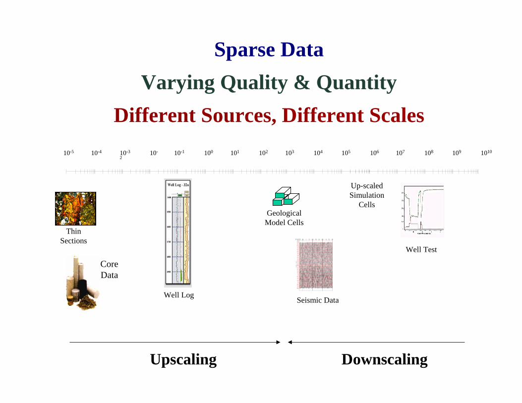
Sparse DataVarying Quality & Quantity

Different Sources, Different Scales

Upscaling Downscaling

10-5 10-4 10-3 10-2

10-1 100 101 102 103 104 105 106 107 108 109 1010

Thin Sections

Core Data

Well Log

Geological Model Cells

Up-scaled Simulation

Cells

Well Test

Seismic Data

Multiscale Approach

• Detailed, heterogeneous reservoir models• Unstructured grids• Robust & reasonable closure• Scalable parallel computation• Conservative on coarse scale• Conservative on fine scale (Reconstruction)• Finite-Volume Framework

MSFV Components:Dual Basis Functions

vDual n 1, v~ =Φv

• Unit pulse at the vertex• Reduced BC

Dual Coarse Cell

Solve:

3

1

4

20)( =∇⋅∇ pλ

21

3 4

MSFV Components:Coarse Grid Operator

ccc fpT =∇⋅∇ )(

Use information from the basis functions to compute the coarse scale transmissibility.

MSFV Components:Primal Basis & Reconstruction

j

j

cj

f pp 5

9

15 Φ=∑

=

Dfp =∇⋅∇ )(λDC

A B

1 2 3

4 5 6

7 8 99 1, j 5 =Φ j

10x22

10x22

20x44

20x44

60x220

60x220

GPRS Overview

• Multiple-purpose research simulator• Modular, object-oriented C++ code• Generalized compositional • AIM• Unstructured grids• Multi-stage Preconditioning for Linear Solver• Multi-level block data structures for preconditionersand Krylov solvers• Advanced well models• Multiple-point flux• Efficient coupling with energy equation

StdWell

MSWell

Grid

Fluid

Rock

Solve r

Fie ld

Re servoir

Smart Well

SimMaster

SurFac Well

Facilities

Adaptive Implicit Model

• Adaptive Implicit Method (AIM) • low flow rate region

• implicit pressure and • explicit saturation (IMPES)

– high flow rate region• fully implicit (FIM) model

FIM

IMPES

AIM: IMPES + FIM

AIM (Adaptive Implicit Method)SPSSPSSPSPSSPPSSP

Cell7

Cell6

Cell5

Cell4

Cell3

Cell2

Cell1

9 1 4

diagonal

off-diag

633

Fundamental physics





Opt

imiz

atio

n

Nature is Not Smooth

Reservoir Properties .• Complex Structures.• Multiple Facies.• Hierarchy of Scales.• Complex Correlation Structures.• High Variability

(even if statistically homogeneous).

Levels of Uncertainty

• Geologic Scenario

• Large-scale objects

• Sub-layer Correlation Patterns

• means, variances, correlation lengths.

• Small-Scale Heterogeneity

• Property Definition (Geostatistics).

Optimization under uncertainty

• Optimization of the injection process• Deploy cost effective smart wells.• Maintain desired flow rates within the formation.• Injection in the favorable parameter range.• Targeted injection.

• Achieve optimization with,• Genetic algorithms (GA) to optimize the well location and to determine the optimal type of well (i.e., monobore, dual-lateral, tri-lateral, etc).

• Adjoint technique to optimize the operation of wells already in place (i.e., to determine injector BHPs as a function of time to optimize cumulative oil or NPV).

Genetic Algorithms Optimization

• Stochastic optimization methods inspired by natural genetics and Darwinian selection

• Combine the parameters of “good individuals” within a given population to create new individuals, in an iterative way

• Evolution of the population from one iteration (generation) to another, until convergence is reached

• Combines “survival of the fittest” with stochastic information exchange (crossover, mutations)

Optimizer flowchart

new population

Check constraints

invalid

Generate random population

Input parameters / constraints

valid


Evaluate the fitness of valid individuals (Eclipse, proxies ...)

Determine a penalty value

Rank population

Select individuals, mate parents,

reproduceOutput result

Check convergence

(Burak Yeten, Vincent Artus)


Characteristic features

• “Good” parameter values difficult to generalize.

• High crossover probability beneficial.

• High mutation probability provides variety.

• Selection of the fittest individuals takes advantage of

good solutions

• Genetic algorithm allows escape from a local minimum.

• Optimization process dependent on:• Selection strategy • Crossover probability• Mutation probability

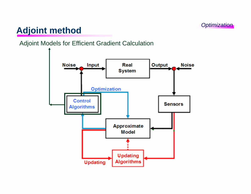
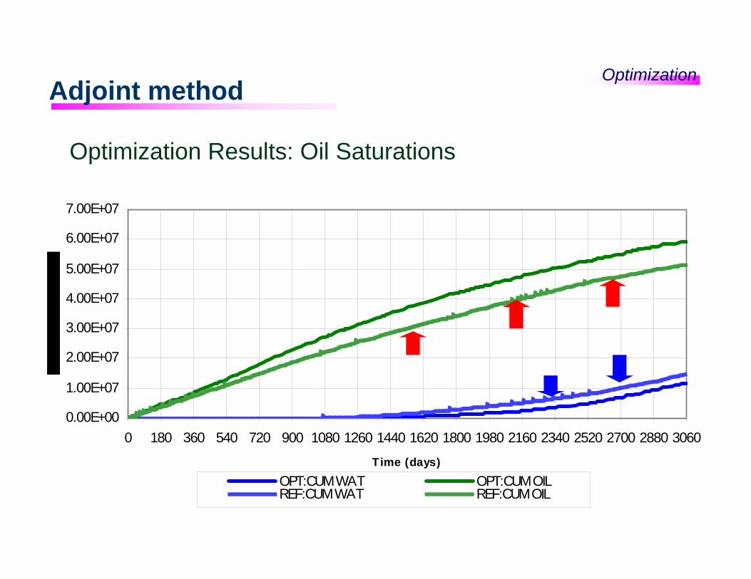
Adjoint methodOptimization

• Efficient calculation of gradients: use of optimal control theory.

• Efficient techniques for handling model uncertainty.Polynomial Chaos and Karhunen-Loeve expansions

• Incorporates prior knowledge about the dynamic system.

• Creates robust proxies to the dynamic system.

• Includes the dynamic system as a constraint.

• Exploits the recursive nature of the dynamic system to efficiently calculate gradients.

• Efficient model updating – Bayesian inversion, K-L expansions and adjoints


Optimization under Uncertainty

Uncertainty Reduction


Adjoint Models for Efficient Gradient Calculation

Adjoint method Optimization

Optimization Results: Oil Saturations

0.00E+00

1.00E+07

2.00E+07

3.00E+07

4.00E+07

5.00E+07

6.00E+07

7.00E+07

0 180 360 540 720 900 1080 1260 1440 1620 1800 1980 2160 2340 2520 2700 2880 3060

Time (days)OPT:CUM WAT OPT:CUM OILREF:CUM WAT REF:CUM OIL


Efficient Uncertainty Propagation with Polynomial Chaos


NPV Distribution from PCE and MC

4 4.5 5 5.5 6 6.5

x 107

0

5

10

15

20

25

30

35

40

45

50NPV from PCE

NPV4 4.5 5 5.5 6 6.5

x 107

0

5

10

15

20

25

30

35

40

45

50NPV from Montecarlo

NPV


Efficient Model Updating with Bayesian inversion and Karhunen-Loeve expansions


− Adjoint models provide an efficient means to calculate gradients.

− The K-L expansion, Bayesian inversion and adjoint models provide an efficient algorithm for model updating under geological constraints

− Polynomial chaos expansions provide an efficient means for uncertainty propagation, while allowing a “black box” approach

− Approximate parameter fields may be adequate for obtaining near optimal trajectories of the controls

− Since adjoint models are used both for optimization and model updating, many components of the code can be reused, resulting in added efficiency

• Essential physical mechanisms relating to fundamental hydrodynamic instability have been evaluated.• Understand their interaction with heterogeneity and as well as study the influence of geochemistry, adsorption, dissolution, precipitation and mineralization.

• Multiscale method for efficient calculations at the field scale.• Evolve GPRS for efficient calculation of injection and long term storage problems.

• For CO2 problems, we can use GAs to optimize well placement and type and adjoint procedures to optimize the CO2 injection operation. • Smart wells for oil field problems, have downhole valves (for injection control) and sensors (which can provide data to be used for history matching).

Future directions

Date post:	10-Mar-2018
Category:	Documents
Upload:	phunglien
View:	222 times
Download:	4 times

Numerical Simulation of CO2 Sequestration in Sequestration in Subsurface Formations Amir Riaz, ......

Documents