Page 1
Numerical Simulation of Dynamic Contact Angles and Contact Lines in Multiphase
Flows using Level Set Method
by
Premchand Pendota
A Thesis Presented in Partial Fulfillmentof the Requirements for the Degree
Master of Science
Approved July 2015 by theGraduate Supervisory Committee:
Marcus Herrmann, ChairKonrad Rykaczewski
Kangping Chen
ARIZONA STATE UNIVERSITY
August 2015
Page 2
ABSTRACT
Many physical phenomena and industrial applications involve multiphase fluid flows
and hence it is of high importance to be able to simulate various aspects of these flows
accurately. The Dynamic Contact Angles (DCA) and the contact lines at the wall
boundaries are a couple of such important aspects. In the past few decades, many
mathematical models were developed for predicting the contact angles of the inter-
face with the wall boundary under various flow conditions. These models are used
to incorporate the physics of DCA and contact line motion in numerical simulations
using various interface capturing/tracking techniques. In the current thesis, a simple
approach to incorporate the static and dynamic contact angle boundary conditions
using the level set method is developed and implemented in multiphase CFD codes,
LIT (Level set Interface Tracking) (Herrmann (2008)) and NGA (flow solver) (Des-
jardins et al. (2008)). Various DCA models and associated boundary conditions are
reviewed. In addition, numerical aspects such as the occurrence of a stress singular-
ity at the contact lines and grid convergence of macroscopic interface shape are dealt
with in the context of the level set approach.
i
Page 3
ACKNOWLEDGEMENTS
I would like to thank my adviser Dr. Marcus Herrmann for consistently sup-
porting me in understanding various technical concepts and inspiring me to be more
productive. I would also like to thank Dr. Konrad Rykaczewski for providing some
insights into experimental aspects of this work and a few experimental images (Figure
1.1) presented in this thesis. I also thank Dr. Kangping Chen for serving as a com-
mittee member and helping me learn various concepts used in this work through his
Continuum Mechanics course. I thank Carlos Ballesteros and Zechariah Jibben for
proofreading the draft and providing invaluable suggestions. I am fortunate to have
worked with very talented students at ASU Multiphase Research Lab who helped me
on numerous occasions.Finally, I would like to thank my parents for supporting my
education.
ii
Page 4
TABLE OF CONTENTS
Page
LIST OF FIGURES . . . . . . . . . . . . . . . . . . . . . . . . . . . . . . . . . . . . . . . . . . . . . . . . . . . . . . . . v
CHAPTER
1 Introduction. . . . . . . . . . . . . . . . . . . . . . . . . . . . . . . . . . . . . . . . . . . . . . . . . . . . . . . . . 1
1.1 Motivation . . . . . . . . . . . . . . . . . . . . . . . . . . . . . . . . . . . . . . . . . . . . . . . . . . . . . 1
1.2 Thesis outline . . . . . . . . . . . . . . . . . . . . . . . . . . . . . . . . . . . . . . . . . . . . . . . . . . 3
2 Governing physics . . . . . . . . . . . . . . . . . . . . . . . . . . . . . . . . . . . . . . . . . . . . . . . . . . . 4
2.1 Multiphase flow governing equations. . . . . . . . . . . . . . . . . . . . . . . . . . . . . . 4
2.2 Dynamic contact angles/lines . . . . . . . . . . . . . . . . . . . . . . . . . . . . . . . . . . . . 5
3 Numerical Methods . . . . . . . . . . . . . . . . . . . . . . . . . . . . . . . . . . . . . . . . . . . . . . . . . . 7
3.1 Level set method for interface capturing. . . . . . . . . . . . . . . . . . . . . . . . . . 7
3.2 Level Set Interface Tracking (LIT) code . . . . . . . . . . . . . . . . . . . . . . . . . . 10
3.3 Flow solver (NGA) . . . . . . . . . . . . . . . . . . . . . . . . . . . . . . . . . . . . . . . . . . . . . 10
3.4 Algorithm for solving a multiphase CFD problem . . . . . . . . . . . . . . . . . 11
4 Mathematical models for contact angles. . . . . . . . . . . . . . . . . . . . . . . . . . . . . . . 12
4.1 Static Contact Angle (SCA) model. . . . . . . . . . . . . . . . . . . . . . . . . . . . . . . 12
4.2 Hydrodynamic theory and dynamic contact angle models. . . . . . . . . . 12
4.2.1 HT and no–slip condition . . . . . . . . . . . . . . . . . . . . . . . . . . . . . . . . . 13
4.2.2 Voinov model . . . . . . . . . . . . . . . . . . . . . . . . . . . . . . . . . . . . . . . . . . . . 14
4.2.3 Cox model . . . . . . . . . . . . . . . . . . . . . . . . . . . . . . . . . . . . . . . . . . . . . . 15
4.2.4 Mesh dependent DCA model by Afkhami et al. (2009) . . . . . . 16
5 Proposed method for prescribing contact angle BC in level set method. . . 17
5.1 Existing methods for prescribing CA boundary condition. . . . . . . . . . . 17
5.2 Proposed method for prescribing Contact Angles. . . . . . . . . . . . . . . . . . 19
5.3 Extension to 3D problems. . . . . . . . . . . . . . . . . . . . . . . . . . . . . . . . . . . . . . . 22
iii
Page 5
CHAPTER Page
5.4 Results and observations . . . . . . . . . . . . . . . . . . . . . . . . . . . . . . . . . . . . . . . . 23
6 Grid convergence of interface profiles . . . . . . . . . . . . . . . . . . . . . . . . . . . . . . . . . . 29
6.1 Effects of reinitialization on CA implementation . . . . . . . . . . . . . . . . . . 29
6.2 Stress singularity at contact line . . . . . . . . . . . . . . . . . . . . . . . . . . . . . . . . . 32
6.3 Grid convergence using slip boundary condition . . . . . . . . . . . . . . . . . . . 35
6.4 Implementation of dynamic contact angle model . . . . . . . . . . . . . . . . . . 38
7 Conclusions . . . . . . . . . . . . . . . . . . . . . . . . . . . . . . . . . . . . . . . . . . . . . . . . . . . . . . . . . 39
7.1 Future work . . . . . . . . . . . . . . . . . . . . . . . . . . . . . . . . . . . . . . . . . . . . . . . . . . . . 39
REFERENCES . . . . . . . . . . . . . . . . . . . . . . . . . . . . . . . . . . . . . . . . . . . . . . . . . . . . . . . . . . . . 41
iv
Page 6
LIST OF FIGURES
Figure Page
1.1 Experimentally observed contact angles . . . . . . . . . . . . . . . . . . . . . . . . . . . . . . 2
2.1 Contact angle definition . . . . . . . . . . . . . . . . . . . . . . . . . . . . . . . . . . . . . . . . . . . . 5
2.2 Apparent contact angle . . . . . . . . . . . . . . . . . . . . . . . . . . . . . . . . . . . . . . . . . . . . . 6
4.1 Viscous bending predicted by hydrodynamic theory. . . . . . . . . . . . . . . . . . . 13
5.1 Straight line ghost interfaces to implement CA BC. . . . . . . . . . . . . . . . . . . . 18
5.2 Wall boundary cell. . . . . . . . . . . . . . . . . . . . . . . . . . . . . . . . . . . . . . . . . . . . . . . . 20
5.3 Curvature calculation in wall adjacent cell. . . . . . . . . . . . . . . . . . . . . . . . . . . 21
5.4 3D drop on a Wall. . . . . . . . . . . . . . . . . . . . . . . . . . . . . . . . . . . . . . . . . . . . . . . . . 22
5.5 Contact angle calculation in 3D. . . . . . . . . . . . . . . . . . . . . . . . . . . . . . . . . . . . . 23
5.6 Test case for prescribing SCA. . . . . . . . . . . . . . . . . . . . . . . . . . . . . . . . . . . . . . . 24
5.7 Planar interface test for prescribing static contact angle. . . . . . . . . . . . . . 26
5.8 Temporal evolution of the interface shape with θleft = 600, θright =
1200. . . . . . . . . . . . . . . . . . . . . . . . . . . . . . . . . . . . . . . . . . . . . . . . . . . . . . . . . . . . . . 27
5.9 Initial curvature values for straight line interfaces . . . . . . . . . . . . . . . . . . . . 28
6.1 Effect of reinitialization on steady state profile. . . . . . . . . . . . . . . . . . . . . . . 31
6.2 Moving contact line in a shear induced flow . . . . . . . . . . . . . . . . . . . . . . . . . . 33
6.3 Divergence of contact line height with no – slip condition. . . . . . . . . . . . . . 34
6.4 Grid convergence of contact line height with slip model . . . . . . . . . . . . . . . 37
v
Page 7
Chapter 1
INTRODUCTION
1.1 Motivation
Multiphase flows can be found in many natural processes and industrial applica-
tions. Some examples for flows found in nature include rain drops falling through
the atmosphere, gas bubbles in water, free surface flows and dust particles floating
in the air. Multiphase flows also have numerous industrial applications such as, flow
through porous media, atomizers, combustion, transport of dispersed solid particles
in fluids and liquid sprays are a few of many applications.
Different phases in multiphase flows are separated by an interface, which is a
physical and mathematical discontinuity on the continuum scale, as the physical
properties of the fluid system change suddenly across the interface. In most of these
applications, tracking the deformation or motion of the interface is of high interest;
and there are several approaches available to understand the same, which are discussed
in the succeeding chapters. When the interface touches the wall boundaries of the
flow domain, a contact angle is formed between the wall boundary and the interface.
The region common to the interface and the wall is called the Contact Line (CL)
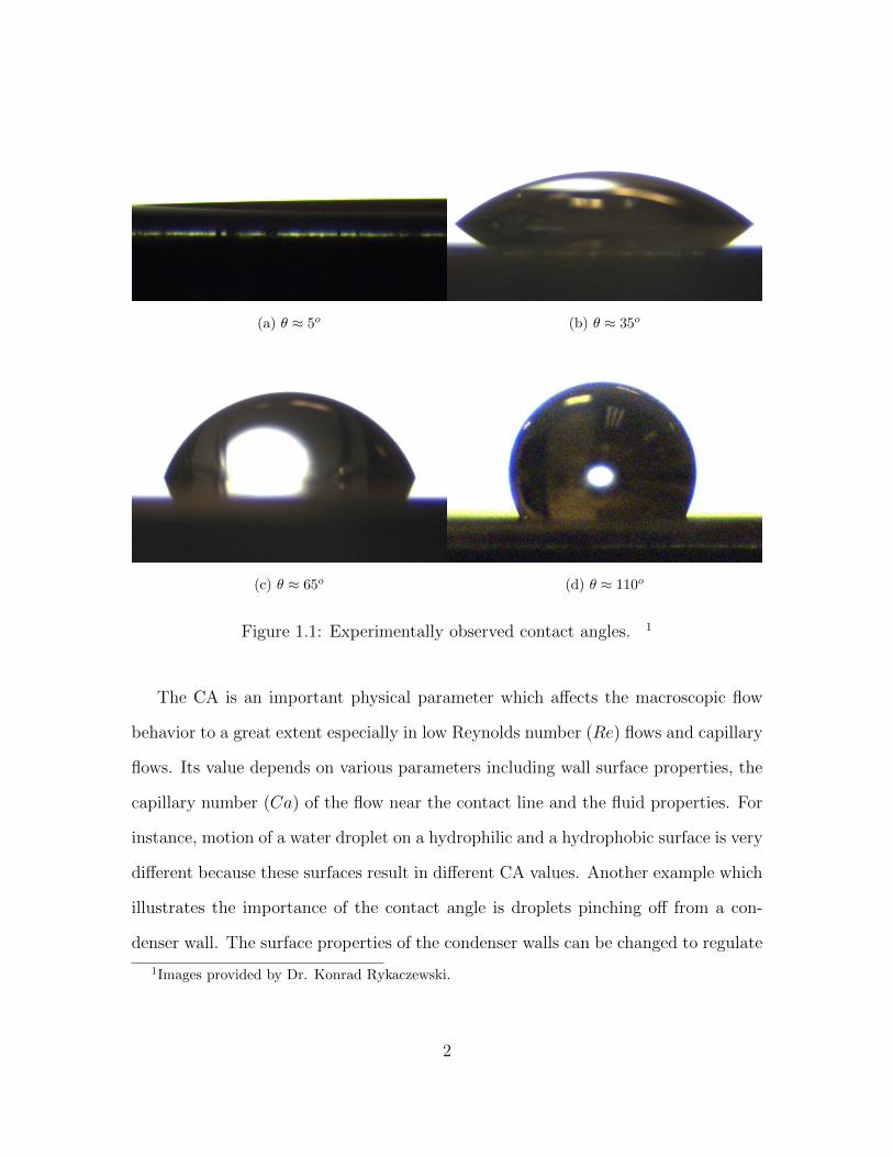
(contact point in a two – dimensional (2D) model). Fig. 1.1 shows different Contact
Angles (CA) observed experimentally for different surface and liquid properties.
1
Page 8
(a) θ ≈ 5o (b) θ ≈ 35o
(c) θ ≈ 65o (d) θ ≈ 110o
Figure 1.1: Experimentally observed contact angles. 1
The CA is an important physical parameter which affects the macroscopic flow
behavior to a great extent especially in low Reynolds number (Re) flows and capillary
flows. Its value depends on various parameters including wall surface properties, the
capillary number (Ca) of the flow near the contact line and the fluid properties. For
instance, motion of a water droplet on a hydrophilic and a hydrophobic surface is very
different because these surfaces result in different CA values. Another example which
illustrates the importance of the contact angle is droplets pinching off from a con-
denser wall. The surface properties of the condenser walls can be changed to regulate
1Images provided by Dr. Konrad Rykaczewski.
2
Page 9
the pinch–off process of the droplets (Walpot et al. (2007)) to improve the efficiency
of the condenser. Thus, Computational Fluid Dynamic (CFD) studies involving such
problems should incorporate the CA physics accurately to obtain physically valid
results. In further sections, it is shown that the CA value which is prescribed as a
Boundary Condition (BC) does impact the macroscopic interface shape to a great
extent, in the numerical simulation of multiphase flows.
1.2 Thesis outline
The objective of the current work is to incorporate the physics of the CA and
CL in multiphase CFD simulations using the Level Set Method (LSM). The resulting
methods are added to the LIT (Level set Interface Tracking) (Herrmann (2008)) and
NGA (flow solver) (Desjardins et al. (2008)) codes. First, a procedure to prescribe
a given CA as a level set method boundary condition is developed. Some test cases
which can be used to verify if the approach results in a correct contact angle treatment
are presented. Then, the existing DCA models are reviewed and the ones which are
most widely used are incorporated in LIT and NGA. In addition to prescribing the
CA, grid convergence of interface profiles is studied and some modifications with
physical basis are made to the BCs of the flow solver, in order to achieve the same.
3
Page 10
Chapter 2
GOVERNING PHYSICS
2.1 Multiphase flow governing equations.
In this section the governing equations of two – phase flows, which are solved using
the CFD codes are presented. The governing equations for an unsteady, incompress-
ible, immiscible two phase fluid systems in vectorial notations are as follows:
1. Conservation of mass
5 · u = 0 (2.1)
2. Conservation of momentum
∂u
∂t+ u · 5u = −5p
ρ+
1
ρ5 ·(µ(5u +5Tu)) + g +
1
ρTσ (2.2)
Where u is velocity vector, p is the pressure, ρ is the density, µ is the viscosity, g is
the gravity force and Tσ is the surface tension force.
As both fluids are considered to be incompressible, the continuity equation results
in a divergence–free condition on the velocity field. The key difference in two–phase
flow momentum equation compared to that of the single phase flow is the inclusion of
the surface tension force term Tσ. The surface tension force is a singular force acting
only at the interface. This is given by Eq. 2.3,
Tσ = σκδ(x− xf )n (2.3)
where xf is the location of interface, n is the normal vector and σ is the surface
tension coefficient. σ is modeled to be a constant value on the entire surface of the
4
Page 11
interface. In addition, a Kronecker delta function is introduced to make it physically
consistent (acting only at the interface). The numerical code details and algorithms
are presented in the following chapters.
2.2 Dynamic contact angles/lines
In this section, some relevant definitions and physics of the CAs are presented.
The CA may be defined as the angle made by the interface at the wall, as shown in
Fig. 2.1 for a 2D case. The CA is a multi–scale property and hence, there is a length
scale involved when defining the same. For example, for an interface shown in Fig.
2.2, the CA made by the interface in the microscopic length scale (lm) is different from
that observed at a macroscopic length scale (L). The microscopic angle in general
is denoted by θw and the macroscopic CA or the Apparent Contact Angle (ACA) is
denoted by θapp. Note that the CA observed experimentally is typically θapp.
Figure 2.1: Contact angle definition
5
Page 12
Figure 2.2: Apparent contact angle
If the interface is at rest relative to the wall boundary, θw is considered to be a
Static Contact Angle (SCA) represented by θs. This angle depends on the material
properties of the wall and the fluids in the system. Although θw is typically assumed
to be constant (= θs) for a given fluids and solid system, it was found that its
value depends on the velocity of the interface (thus, Ca) as well (Blake and Haynes
(1969)). This angle that the interface makes when it is in motion relative to the
wall, is defined as the Dynamic Contact Angle (DCA), denoted by θd. θd depends
on θs, Ca, macroscopic flow structure and also flow in the vicinity of the contact line
(Shikhmurzaev (2006), Blake et al. (1999)).
For any numerical simulation involving contact lines, the CA is to be prescribed
as a boundary condition at every time step. In case of macroscopic simulations, θapp
is prescribed instead of θw as a boundary condition, to obtain the correct macroscopic
interface profile. There are different models available to calculate θapp, of which the
widely used models are presented in the following chapters.
6
Page 13
Chapter 3
NUMERICAL METHODS
In this chapter, a brief overview of the numerical methods used in this study are
presented. For the purpose of solving the Navier – Stokes equations presented in the
Sec. 2.1, the CFD code NGA (Desjardins et al. (2008)) is used. For interface captur-
ing and evaluating interfacial properties including curvature, the Level set Interface
Tracking (LIT) code (Herrmann (2008)) is used.
3.1 Level set method for interface capturing.
There are two general approaches used to track the temporal evolution of the inter-
face in multiphase flows; namely, explicit and implicit methods. In explicit methods,
the interface is tracked explicitly, for instance, by tracking the marker points used to
represent the interface (Hyman (1984)). On the other hand, in implicit methods, the
interface is embedded in a scalar field and the entire scalar field is updated dynam-
ically to capture the interface motion. The Level Set Method (LSM) is one of the
implicit methods that can be used for this purpose.
The LSM for capturing evolving fronts was first introduced by Osher and Sethian
(1988). In this method, the interface is embedded in a higher dimensional scalar level
set field. At a given time, the interface shape and position are obtained implicitly
through a constant level set (iso–surface) of a function used to represent the interface.
Different functions can be used to represent an interface in LSM. For example, a
signed distance function (Chopp (1993)) and a hyperbolic tangent function (Olsson
and Kreiss (2005)) are widely used to represent the interface. In the current work, a
signed distance function is used to represent the interface. Using this function, at any
7
Page 14
given point, the LS value (φ) is given by the shortest signed distance to the interface.
This function also has the property given by Eq. 3.1. The sign of the φ value is used
to differentiate between fluid zones in which the point lies. Hence the zero iso–surface
of the LS field represents the interface.
| 5 φ| = 1 (3.1)
Once the LS field is initialized using a signed distance function, the interface is
transported implicitly by transporting the entire LS field. Since the transport of the
interface in immiscible fluids involves only advection, the LS transport equation is
given by Eq. 3.2 (scalar advection). Also, the interface is advected with the local
flow velocities and hence the same are used in the advection equation. The required
velocities are obtained from the flow solver at every time step. As can be observed,
the advection equation is a Hamilton – Jacobi equation of hyperbolic nature. Hence,
mathematically the information travels from the interface along the characteristics in
a normal direction.
∂φ
∂t+ u.5 φ = 0 (3.2)
Once the LS field is advected, the LS values at different points are not guaranteed
to remain a signed distance function. While the simulation can still be continued,
it is important to maintain a signed distance function property (Eq. 3.1) in order
to maintain a constant thickness of the interface and for an accurate evaluation of
curvature, as solving Eq. 3.2 could result in steep gradients in φ field (Sussman et al.
(1994)). If there are errors in the curvature calculation, it leads to spurious currents
near the interface (Herrmann (2008)). Hence the signed distance property is to be
restored by reinitializing the LS field.
Various approaches were developed to reinitialize the LS field. One of the widely
used methods and the one used in this work is Partial Differential Equation (PDE)
8
Page 15
based reinitialization, proposed by Sussman et al. (1994) given by Eq. 3.3. The key
advantages of PDE based reinitialization over other methods are ease of parallelization
and computational inexpensiveness. In this approach, at every time step, Eq. 3.3 is
solved until reaching steady state in pseudo–time τ . To avoid moving the zero LS, a
sign function can be used, which is given by Eq. 3.5. This is formulated such that
the zero iso–surface (φ0(x)) remains the same before and after reinitialization. Also,
a smoothed form of the sign function, as in Eq. 3.5 is used for numerical purpose
of smoothing the jump discontinuity in the ρ or µ values across the interface, which
results in an interface with finite thickness.
∂φ
∂τ= S(φ0)(1−
√φx
2 + φy2) (3.3)
φ0(x) = φ(x, 0) (3.4)
Sε(φ0) =φ0√
φ02 + ε2
(3.5)
Similar to the advection equation of LS field, Eq. 3.3 is a time evolution equation.
Since this method relies on solving a PDE to steady state, numerical errors due
to round–off, truncation or approximation are inevitable. This leads to change in
φ values at the zero iso–surface which effectively move the interface and result in
changes to the volumes of individual fluids. Hence to limit these errors, reinitialization
is performed only when appropriate trigger conditions are met by the φ field. One
way is to reinitialize only when the LS field diverges from being a distance function
(3.1) as developed by Gomez et al. (2005). This is given by Eq. 3.6,
max(| 5 φ|) > αmax or min(| 5 φ|) < αmin (3.6)
where αmin and αmax are real constants. In addition, the minimum and maximum
number of pseudo iterations to be performed in each time step can also be used as a
trigger.
9
Page 16
3.2 Level Set Interface Tracking (LIT) code
The Level Set Interface Tracking (LIT) code uses a cell centered equidistant Carte-
sian grid and Finite Difference Method (FDM) to solve LS equations including ad-
vection and reinitialization. In addition, it also calculates other required quantities
like curvature (κ). The code employs the Refined Level Set Grid (RLSG) method de-
veloped by Herrmann (2008). The key idea behind this approach is that an auxiliary
equidistant Cartesian grid with higher resolution compared to the flow solver grid can
be used to accurately define and track the interface motion. Thus interfaces which
are highly curved can be represented more accurately compared to a standard LS
approach, which helps in accurate calculation of curvature values. In order to achieve
a grid with a manageable size, a two–level narrow band approach (Adalsteinsson and
Sethian (1995) and Jiang and Peng (2000)) is used. In addition, for the LS advection
and reinitialization, fifth–order WENO Scheme of Jiang and Peng (2000) coupled
with TVD RK of third–order accuracy (Shu (1988)) are used for numerical stability.
3.3 Flow solver (NGA)
NGA is a finite–volume flow solver on a structured staggered mesh. It implements
a second order conservative scheme for the spatial quantities as in Morinishi et al.
(2004). For temporal quantities, second order integration is implemented as in Pierce
(2001). It also has the balanced force algorithm (Francois et al. (2006)) implemented
to reduce the spurious currents caused by curvature errors. Additional details about
the flow solver can be found in Desjardins et al. (2008).
NGA uses Continuum Surface Force (CSF) model to calculate surface tension
force in an explicit way and thus, imposes capillary time step limitation (Brackbill
et al. (1992)). This limitation is in addition to the standard Courant – Friedrichs –
10
Page 17
Lewy (CFL) condition for Navier – Stokes equations and is given by,
4t ≤ 4tcap =
√(ρ1 + ρ2)43
4πσ(3.7)
where 4t is the time step, 4tcap is the capillary time – step, 4 is the characteristic
grid size of the flow solver, ρ1 and ρ2 are the densities of the two fluids and σ is the
surface tension coefficient.
3.4 Algorithm for solving a multiphase CFD problem
The NGA and LIT codes are coupled in order to simulate the time evolution of the
interface. NGA requires the curvature (κ) from the LIT grid in order to evaluate the
surface tension force (Tσ). NGA also required the interface position to calculate the
physical parameters including density and viscosity at a given point to calculate the
flow variables. LIT obtains the velocities used for advection from NGA. The entire
simulation process can be summarized using the following algorithm:
Algorithm 1 Solving multiphase CFD problem
Initialize the flow solver (velocities and pressure).
Set the BCs in the Flow Solver.
Initialize the level set field
while (time ≤ end time) do
Advect the interface using velocities from flow solver.
Reinitialize the LS Field
Import interface position and curvature data into flow solver
Advance the Flow Solver simulation by one time step
end while
11
Page 18
Chapter 4
MATHEMATICAL MODELS FOR CONTACT ANGLES.
In this chapter, various mathematical models which are widely used in the literature
to predict the Contact Angle (CA) made by the interface at the wall are presented.
4.1 Static Contact Angle (SCA) model.
One of the simplest CA models is for evaluating the SCA (θs, defined in 2.2) was
developed by Young (1805) for a given solid – liquid – gas system. The model is given
by Eq. 4.1,
γsv − γsl = γlv cos θ (4.1)
where γsv, γsl, γlv are the interfacial surface free energies for solid – vapor, solid – liquid
and liquid – vapor pairs respectively. This equation is only valid for smooth surfaces
and liquid – gas type of systems alone. Cassie and Baxter (1944) have developed a
more accurate model considering the surface imperfections as well.
4.2 Hydrodynamic theory and dynamic contact angle models.
The multi–scale property of the CA is introduced in Sec 2.2, because of which,
if one conducts an experiment to observe the CA in a multiphase system, it can be
found that the observed apparent CA (θapp) is not the same as the θw at microscopic
level. Hence when performing numerical simulations, if a Direct Numerical Simulation
(DNS) is performed (resolving all the length scales involved), θw itself is sufficient to
obtain the right flow structure, without any further modeling of CA (Sui and Spelt
(2013)). A DNS is many times not practical mainly because it is computationally
12
Page 19
very expensive and hence, θapp needs to be modeled which is then used as a boundary
condition. If modeled accurately, θapp BC should result in a similar macroscopic
interfacial structure as that of using θw as a boundary condition in a DNS.
There are currently two approaches to develop a DCA model for θapp, Hydro-
dynamic Theory (HT) and the Molecular – Kinetic theory. A summary of both
approaches can be found in Blake (2006). In the current research work, models based
on HT are used. The key aspect of HT is that θapp is primarily different from the
θw because of viscous bending of the interface in the intermediate mesoscopic range
(Blake (2006)). Thus, HT predicts that there are three regions in which the interface
bending occurs, resulting in a length scale dependent CA (θ(r)), as shown in Fig.
4.1. Here r is the distance from the point where θ is measured to the contact line.
The length scales corresponding to the regions are microscopic (inner), mesoscopic
(intermediate) and macroscopic (outer).
Figure 4.1: Viscous bending predicted by hydrodynamic theory.
4.2.1 HT and no–slip condition
One issue with classic HT is the incompatibility of the dynamic contact line with
the standard no–slip BC used for solving the flow equations. As it is known, with
13
Page 20
the no–slip condition, the velocity of fluid or contact line on the wall is equal to that
of the wall. Thus the no–slip condition on the wall leads to a non–integrable stress
singularity at the contact line and thus the solution cannot be calculated near the
contact line (Cox (1986)). One approach is to use a slip BC for velocity in the contact
line region on the wall to relax the stress singularity and solve the problem.
A free–slip condition was proposed by Hocking (1977), for the contact line region
(distance slip length (λ) around the contact line) and standard no–slip condition in the
single phase region. This results in zero shear stress along the wall near the contact
line and hence; allows for a solution to be calculated. Numerically, this implies setting
the velocities in the ghost cells equal to that of the corresponding interior cells. Other
approaches include making the shear stress finite and non–zero by implementing a
slip BC developed by Navier (1823), as given by the Eq. 4.2,
ucl − uw = λ∂u
∂y(4.2)
where ucl is the velocity of the CL along the wall, uw is the velocity of wall boundary,
λ is the slip length and (∂u
∂y) is the shear stress component tangential to the wall.
When λ = 0, it results in a no – slip condition and when λ = ∞, it results in a free
slip condition.
These slip models are easy to implement but are not accurate enough to capture
the actual physics of contact line motion, as verified experimentally by Wilson et al.
(2006). There are other recent slip models as well (Shikhmurzaev (2006)) which try
to include the flow effects in the vicinity of the contact line.
4.2.2 Voinov model
The Voinov (1976) model is one of the earliest DCA models developed using HT,
applicable for a liquid–gas system. The model was derived considering only the inner
14
Page 21
and outer regions of Fig. 4.1 and in the limit Ca→ 0, shown in Eq. 4.3,
θapp3 − θw3 = 9Ca ln(
L
lm) (4.3)
where θapp <3π
4, L is the macroscopic length scale and lm is the microscopic length
scale. One of the main limitations of the model is that it is applicable to only systems
with a liquid – gas interface, where the gas is assumed to be inviscid.
4.2.3 Cox model
Cox (1986) proposed a much more general and complete model for DCA compared
to the existing models. His model is applicable to systems with two viscous fluids and
was obtained considering three regions (as in Fig. 4.1.) similar to that of Hocking
and Rivers (1982). The Navier slip law (Eq. 6.4.) was used to remove the stress
singularity. The key idea of this theory is that, when three regions of expansion are
considered, the solution in the intermediate region is independent of the inner and
outer region solutions, when calculated to the lowest order of Ca. In case of next
higher order of Ca, it was considered that the solution in intermediate region depends
on only one constant from either the inner or outer regions. Once the solution is found
for the intermediate region, it is then matched with the solutions in the inner and
outer regions using asymptotic theories, leading to a general three region solution,
given by Eq. 4.4, which is correct to O(Ca2),
g(θapp) = [g(θw) +Ca ln(ε−1)] +Ca[(f(θw))−1Qi∗ − (f(θapp))
−1Qo∗] +O(Ca2). (4.4)
where
g(θ) =
∫ θ
0
dθ
f(θ, λ)(4.5)
and
f(θ, q) =2 sin θ[q2(θ2 − sin2 θ) + 2q[θ(π − θ) + sin2 θ] + (π − θ)2 − sin2 θ]
q(θ2 − sin2 θ)[(π − θ) + sin θ cos θ] + [(π − θ)2 − sin2 θ](θ − sin θ cos θ)
(4.6)
15
Page 22
Here q is the ratio of viscosities between the two fluids, ε =λ
L, λ is the slip length, L
is the macroscopic length scale and Q∗i and Q∗
o are constants based on the geometry
of the interface in the inner and outer regions respectively. The Eq. 4.4 correct to
O(Ca0) is given by Eq. 4.7. This is currently the most widely used DCA model to
obtain the BC for CA, in macroscopic numerical simulations.
g(θapp) = g(θw) + Ca ln(ε−1). (4.7)
The key limitations of the Cox model are its validity in low Ca flows where surface
tension force dominates the viscous force and in low Re flows where the inertial forces
are negligible compared to the viscous forces. It is also assumed that the slip of the
interface occurs within the slip length (λ) around the contact line and ε is assumed
to be very small.
4.2.4 Mesh dependent DCA model by Afkhami et al. (2009)
In many numerical studies involving DCA and DCL, one of the key challenges is
to obtain grid converging interface profiles. Afkhami et al. (2009) developed a DCA
model which is specifically aimed at obtaining interface profiles which are consistent
at a macroscopic length scale, obtained using different grid resolutions. The modified
DCA model is given by Eq. 4.8,
g(θnum) = g(θapp) + Ca ln(4/2L
) (4.8)
where θnum is the CA boundary condition, 4 is the grid spacing and L is the macro-
scopic length scale. It is important to note that in this model, the θnum is used as
the boundary condition instead of θapp, based on the grid spacing 4. Although a
constant θapp was used in this study, θapp can be calculated using other DCA models
separately. Hence for a given θapp, this model can be used to obtain CA boundary
condition (θnum) which results in a grid converging macroscopic interface profile.
16
Page 23
Chapter 5
PROPOSED METHOD FOR PRESCRIBING CONTACT ANGLE BC IN LEVEL
SET METHOD.
In this chapter some of the approaches taken to apply the contact angle boundary
condition and a simple approach to prescribe a given Contact Angle (CA) as the
Boundary Condition (BC) in level set method (LSM) are presented.
5.1 Existing methods for prescribing CA boundary condition.
One of the earliest approaches in prescribing a CA boundary condition in a LSM
formulation was developed by Sussman and Uto (1998) to study the spreading of a
liquid drop. A static contact angle (θs) obtained from an experimental observation
was used as the CA boundary condition. This CA boundary condition was imple-
mented by a straight line (2D case) extension of the interface (ghost interface) from
the contact line, with the required CA at the wall as shown in Fig. 5.1. The ghost
interface is shown using a blue dashed line which makes the required CA θapp with
the wall. The LS ghost cell values (φg) are then set to signed distance to the ghost
interfaces, wherever a normal can be drawn from the ghost interface to that cell,
represented by blue shaded region. In the ghost cell zones where a normal from the
interface cannot be drawn, represented by gray zone, extrapolated values for φg are
used. This also involves identifying the contact points first by extrapolation of the
interface to the wall. The approach was presented for a 2D problem. Also, a free slip
condition was used at the contact line.
17
Page 24
Figure 5.1: Straight line ghost interfaces to implement CA BC.
Spelt (2005) developed an approach to account for CA hysteresis and also for
multiple contact lines. Although an approach similar to that of Sussman and Uto
(1998) is followed to calculate φg, by using a straight–line extension of the interface
(2D case), the key difference in this work is to prescribe the interface velocity rather
than the CA. The CA model used is reformulated to calculate velocity as the boundary
condition for the contact line. The required interface position and the CA value are
determined iteratively.
Arienti and Sussman (2014) recently implemented the CA physics in a sharp in-
terface approach with an embedded LS field by prescribing the normal at the contact
line. Also, no – slip BC was used which numerically results in a grid dependent slip
length for cell centered φ values. Recently Della Rocca and Blanquart (2014) devel-
oped a modified reinitialization equation to be applied specifically at the boundary
adjacent LS cells (φw) in cases with contact lines in order to prescribe the CA bound-
ary condition and to reduce the spurious currents resulting from curvature errors.
Thus, instead of setting the φg values directly, their modified reinitialization equation
reinitializes the LS field such that the CA BC is imposed at φw. In this study the
free–slip BC was used at the wall with CL.
18
Page 25
5.2 Proposed method for prescribing Contact Angles.
The effect of CA at the wall boundary is mainly important during the calculation
of curvature and in the visualization of the interface shape at the wall at any given
time step. The Neumann BC typically used for the ghost cell LS values (φg) always
results in a 90o contact angle which mostly results in an inaccurate curvature value
and representation of the interface geometry at the boundary. Hence, the idea is
to modify the φg values, such that the right contact angle is prescribed in φw cells.
This should result in correct visualization of interface when plotted and also correct
curvature values automatically.
Prescribing a CA in the φw cells is equivalent to prescribing a normal value at that
point, as for a given CA value, there is a unique normal. The normal at a boundary
cell φw can be calculated using (for a 2D problem),
~N =5φ| 5 φ|
=⇒ Nx =−φx√φx
2 + φy2;Ny =
−φy√φx
2 + φy2;
φx =(φ(i+ 1, j)− φ(i− 1, j))
hx;φy =
(φ(i, j + 1)− φg)hy
; (5.1)
where hx and hy are the grid spacings in x and y directions respectively. Eq. 5.1 is
obtained using standard central differencing to calculate the normal components.
It is important to note that prescribing the normal should be done without al-
tering the φ values inside the flow domain, so that the actual interface is not moved
inadvertently and lead to volume change of individual fluids. Thus, the required nor-
mal can be prescribed by modifying the φg value in Eq. 5.1. If θ is the angle being
prescribed for the interface shown in the Fig. 5.2, the target normal is given by Eq.
5.2.
Nxtar = − cos(π
2− θ) ; Nytar = sin(
π
2− θ) (5.2)
Thus, equating the ratios of target and current normal values and solving for φg,
19
Page 26
Figure 5.2: Wall boundary cell.
we obtain,
φg = φ(i, j + 1) + tan(π
2− θ) · φx · hy (5.3)
where hy is the grid spacing in y–direction. Note that the Eq. 5.3 is valid only for
a 2D case in which the interface is inclined as shown in Fig. 5.2. The expressions
for other θ values can be derived in a similar way by calculating the target normal
components and equating them to the standard normal formulas as in Eq. 5.1.
The curvature (κ) calculation in a LS formulation for a 3D problem is given by
the Eq. 5.4.
κ =φ,xx(φ
2,y + φ2
,z) + φ,yy(φ2,x + φ2
,z) + φ,zz(φ2,y + φ2
,z)
(φ2,x + φ2
y + φ2z)
3/2−2
φ,xyφ,xφ,y + φ,xzφ,xφ,z + φ,yzφ,yφ,z(φ2
,x + φ2,y + φ2
,z)
(5.4)
κ calculation in any cell using Eq. 5.4 involves a 27 point stencil of φ cells (9 in
a 2D problem), when standard central differencing is used. Note that κ calculated
using this formula at any point is the κ of the iso – surface which passes through
20
Page 27
Figure 5.3: Curvature calculation in wall adjacent cell.
the point itself and not that of the actual interface (zero iso–surface). Now consider
κ calculation in φw2 cell as shown in the Fig. 5.3, for a planar interface. In this
example, the CA of the iso–surface through φw2 is assumed to be the same as that
of the prescribed CA. Hence this should result in a κw2 = 0. For this to be true, the
iso–urface through φw1, φw2 and φw3 needs to have the same curvature. Hence the
same CA BC should be applied to calculate φg1 and φg3 in addition to φg2, in order
to avoid curvature errors.
The key difference between this method and the ones proposed earlier in LS ap-
proach is that the φ values are not strictly signed distance functions but are obtained
such that the required normal is imposed at the boundary cells. Hence it can be
considered as prescribing a normal rather than φ values directly.
Note that the angle being prescribed could be a SCA (same in every time step)
or a DCA (varies every time step), but the approach to setting the CA BC remains
the same. Only difference being, when prescribing a DCA, the value is calculated at
every time step of the simulation using any of the previously described models.
21
Page 28
5.3 Extension to 3D problems.
The definition of a contact angle for a 3D interface is not as straight forward as
in a 2D case. In a 3D domain, the contact angle can be defined as the angle between
the tangential surface of the interface and the wall. By this definition, only the z
component of the target normal is varied when CA BC is changed and the x and y
components remain the same, as shown in Fig. 5.5. The rest of the procedure remains
the same in obtaining the φg value (in z direction in this example).
Figure 5.4: 3D drop on a Wall.
22
Page 29
Figure 5.5: Contact angle calculation in 3D.
5.4 Results and observations
In order to test the proposed approach, a simple 2D test case is presented as shown
in Fig. 5.6. A planar interface which is initially horizontal is considered with initial
contact angles being 900 on both left and right walls. Now different CA boundary
conditions are prescribed on opposite walls such that the sum of both the angles is
1800 (in order to obtain a straight line steady state profile). The smallest or largest
angle that can be prescribed in this case depends on the size of the domain. The
true solution is a static straight line with its contact angle values equal to the ones
prescribed in the boundary conditions, as there is no other external or body forces
acting on the system.
23
Page 30
Figure 5.6: Test case for prescribing SCA.
The physical values used for the fluid system are the same as the ones considered
in Afkhami et al. (2009). Both the fluids are chosen to have same densities and
viscosities of 1.0 and 0.25 respectively. Surface tension constant σ is set to 7.5. Also,
the gravitational force is not considered in this problem. These values are chosen
such that the resulting flow has low Re and low Ca. There are two reasons why
these regimes are chosen: to avoid any inertial effects and also to maximize the effect
of surface tension force on the system. The results and comparison with the true
solution is shown in Fig. 5.7.
24
Page 31
(a) θleft = 120o, θright = 60o
(b) θleft = 135o, θright = 45o
25
Page 32
(c) θleft = 60o, θright = 120o
(d) θleft = 45o, θright = 135o
Figure 5.7: Planar interface test for prescribing static contact angle.
26
Page 33
The red line in each plot represents the theoretical steady state solution and the
black line represents the solution obtained using the current method for prescribing
the CA. From the above results it can observed that the steady state profile is visually
very well aligned with the theoretical solution. In this case, at every time step a
constant SCA value is prescribed. The temporal evolution of the interface shape for
the case with θleft = 600 and θright = 1200 is shown in the Fig. 5.8.
Figure 5.8: Temporal evolution of the interface shape with θleft = 600, θright = 1200.
It is important to note that when a contact angle value very different from the
current or local CA value is prescribed, a very high curvature and thus surface tension
force is applied at the contact line suddenly. This could lead to break–up of the
interface at the wall.
A simple test case which can be used to test the SCA BC prescription numerically
is to initialize the LS field with BCs on φ such that the interface has a CA value
equal to the prescribed SCA value. This should result in zero curvature and thus no
contact line motion, if no other forces including gravity are acting. Fig. 5.9 shows
such configurations in the current approach and the corresponding curvature values
initially obtained.
27
Page 34
(a) θleft = 120o, θright = 60o
(b) θleft = 45o, θright = 135o
Figure 5.9: Initial curvature values for straight line interfaces
28
Page 35
Chapter 6
GRID CONVERGENCE OF INTERFACE PROFILES
In the previous chapters, the procedure to implement a given contact angle value
at any time step during the simulation is presented and the approach is tested by
prescribing a fixed SCA value. In real applications, this value becomes a boundary
condition which is obtained from a Dynamic Contact Angle (DCA) model. Some
of the models are discussed in the Ch. 4. In addition to the implemention of a
DCA model, there are a few issues with moving Contact Lines (CL) which are to be
addressed. The first one being the effects of reinitialization of the level set (LS) field
on CA implementation and the second being handling the stress singularity at the
moving CL. These issues are addressed in this chapter and then implementation of a
DCA model is discussed.
6.1 Effects of reinitialization on CA implementation
As it is known, the LS method is not volume conserving by nature, partly because
of reinitialization of the LS field. By solving the reinitialization equation (Eq. 3.3),
the φ values inside the domain are modified such that the distance function property
(Eq. 6.1) is restored. Although the reinitialization equation is formulated to not
move the zero iso–surface, in practice it does move the interface and thus results in
volume change of individual fluids. This is more pronounced in the regions with high
gradients in the φ values, which are inevitable when incorporating the CA BC. Thus
reinitialization is triggered more often when the contact angle value at a given time
step is very different from the prescribed CA BC, as also noted by Della Rocca and
Blanquart (2014), resulting in volume change of individual fluid zones.
29
Page 36
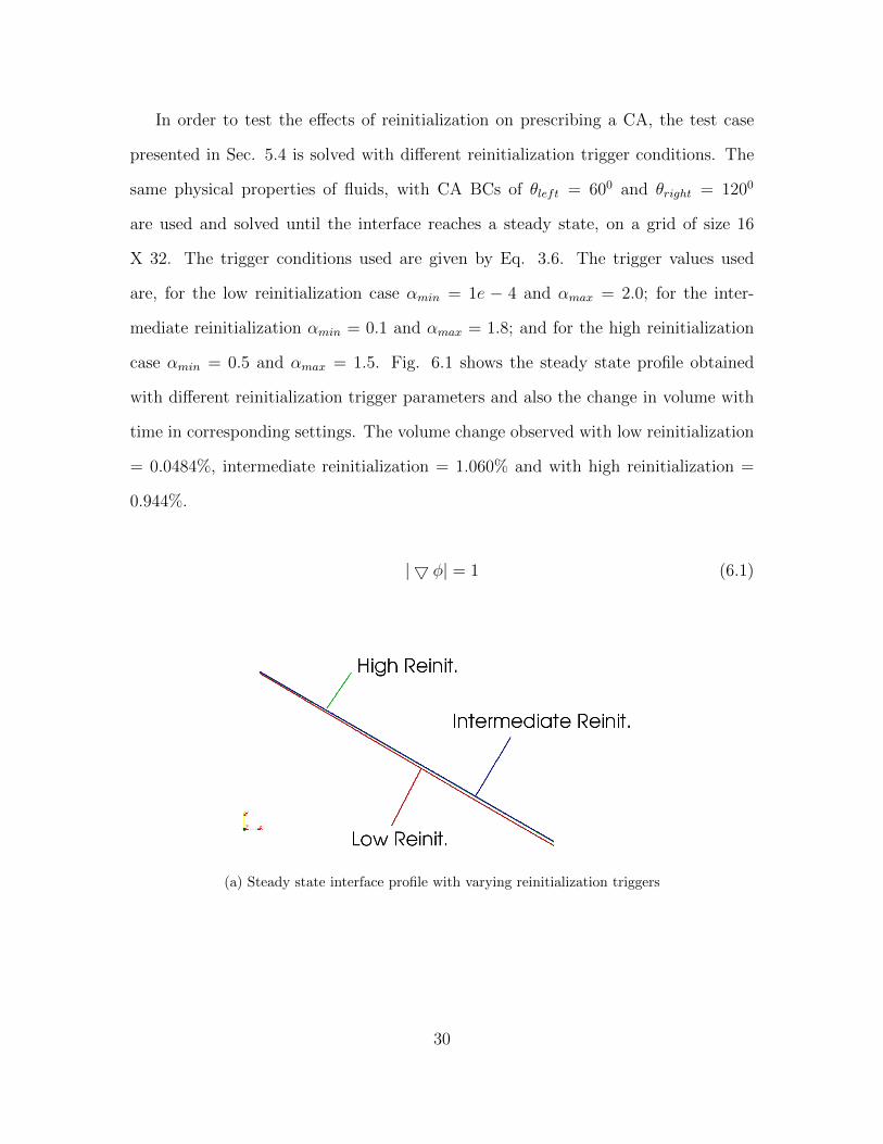
In order to test the effects of reinitialization on prescribing a CA, the test case
presented in Sec. 5.4 is solved with different reinitialization trigger conditions. The
same physical properties of fluids, with CA BCs of θleft = 600 and θright = 1200
are used and solved until the interface reaches a steady state, on a grid of size 16
X 32. The trigger conditions used are given by Eq. 3.6. The trigger values used
are, for the low reinitialization case αmin = 1e − 4 and αmax = 2.0; for the inter-
mediate reinitialization αmin = 0.1 and αmax = 1.8; and for the high reinitialization
case αmin = 0.5 and αmax = 1.5. Fig. 6.1 shows the steady state profile obtained
with different reinitialization trigger parameters and also the change in volume with
time in corresponding settings. The volume change observed with low reinitialization
= 0.0484%, intermediate reinitialization = 1.060% and with high reinitialization =
0.944%.
| 5 φ| = 1 (6.1)
(a) Steady state interface profile with varying reinitialization triggers
30
Page 37
(b) Volume change in time with varying reinitialization
triggers.
Figure 6.1: Effect of reinitialization on steady state profile.
It should be noted that neither the current approach to set the normals nor the
standard Neumann BC necessarily result in φg values which satisfy Eq. 6.1. But
Neumann BC (zero - gradient) results in smoother φ values than setting the normals.
Hence, the proposed approach might trigger the reinitialization procedure more often
than the Neumann BC resulting in volume loss. This can be reduced by making
a small change to the algorithm of advection and reinitialization of φ field; by first
calculating φg using the Eq. 6.1 or using Neumann and then setting the CA boundary
conditions.
31
Page 38
Algorithm 2 Reducing volume change due to reinitialization
Advect the φ values.
Set the φg values using Eq.6.1 or Neumann BC.
Reinitialize the Level Set Field
Set φg values using CA BC.
By making this change, unnecessary reinitialization triggered by the CA BC can
be avoided and a reduction in volume errors can be obtained. This approach is
similar to the modification of te reinitialization equation proposed by Della Rocca
and Blanquart (2014). The difference being, instead of modifying the reinitialization
equation, the φg values are adjusted directly to reduce the reinitialization effect at
the boundary adjacent cells. In the current study, reinitialization is performed every
time step without exceeding 5 pseudo reinitialization time steps in addition to setting
the trigger conditions of αmin = 1e− 4 and αmax = 2.0 as in Eq. 3.6.
6.2 Stress singularity at contact line
One of the key requirements in the implementation of a DCA model is the grid
convergence of interface profile. Although there are many prior studies involving
implementation of DCA in LS and Volume of Fluid (VoF) approaches, only recently
efforts have been made (first by Afkhami et al. (2009)) to address the issue of grid
convergence of the interface profile. It was observed that when a standard no–slip
condition is used, it leads to the divergence of the wall shear stress component and
the interface profile at steady state; at increasing levels of grid refinement (Afkhami
et al. (2009),Sui and Spelt (2013),Shikhmurzaev (2006)).
To test the convergence of the interface profile at steady state with LIT and NGA,
a test case similar to that of the one used in Afkhami et al. (2009), as in Fig. 6.2
32
Page 39
is used. The 2D domain consists of walls on all boundaries. The left wall is moving
in the +y direction with a velocity uw = 1.0 inducing shear into the system. The
interface initially has a CA of 900 and different CA values can be prescribed as a BC,
as discussed in Ch. 5. Since this test case is aimed at testing grid convergence of
interface profile at steady state, only SCA values are prescribed. Also, gravity is not
considered as it reduces the overall height to which the interface rises.
Figure 6.2: Test case: Moving contact line in a shear induced flow.
On the right wall, a free–slip condition with a Neumann BC for φ is applied.
First, the standard Neumann BC on φ which implies a 90o contact angle at the wall
is tested for grid convergence of contact line height (Fig. (6.3)). The overall mass
change in each set up was found to be less than 1%.
33
Page 40
Figure 6.3: Divergence of contact line height with no – slip condition.
From Fig. 6.3 it can be observed that the contact line does not converge with
the standard no–slip BC. The divergence of contact line height is mainly because the
shear stress component along the wall does not converge with grid refinement due
to the no–slip condition. This is the standard BC at walls while solving Navier –
Stokes equations in single phase problems. Numerically, in a staggered grid setup,
this condition is implemented using the ghost cell velocity components as there is no
tangential velocity component calculated on the wall in the standard staggered grid
approach. Thus, by extrapolation, the ghost cell velocity vg is given by Eq. 6.2,
Uw =vi + vg
2=⇒ vg = −vi + 2Uwall (6.2)
where Uwall is the velocity of the wall, vg is the ghost cell velocity and vi is the interior
wall adjacent cell velocity. The corresponding shear stress component tangential to
the wall can be calculated as in Eq. 6.3,
τw ≈∂v
∂x=⇒ τwall ≈
vi − vg4
(6.3)
where τw is the wall shear stress component and 4 is the grid spacing. At steady
state, vi goes to zero. Which implies, with grid refinement, τw increases continuously
without converging to a finite value. Note that the contact line moves because of
34
Page 41
the implicit slip (42
) offered by the staggered velocities and cell centered φ velocities
which are advected. This corresponds to a slip –length of42
, which is obviously grid
dependent. Hence it can be expected that the contact line height does not converge
with standard no–slip condition.
6.3 Grid convergence using slip boundary condition
One approach to handle this stress singularity and remove the implicit slip length
dependence is to use a slip BC with a slip length λ as in Eq. 6.4, as proposed by
Navier (1823). This BC can be implemented using Eq. 6.5 (Afkhami et al. (2009)).
u− uw− = λ(∂u
∂x) (6.4)
ug =2uw 4−(4− 2λ)vi
4+ 2λ(6.5)
Using this value for ug, as opposed to the one derived in Eq. 6.2, reduces the
shear stress singularity and must result in a grid converging interface profile. This
can be verified by evaluating τw as in Sec. 6.2. Thus using the ug value from the slip
condition, the new τw value at steady state can be estimated as in Eq. 6.6. From this
relation it can be observed that as grid refinement increases (4→ 0), the wall shear
stress τw converges to a constant value depending on the value of λ.
(τw)steady ≈−2uw4+ 2λ
(6.6)
It was observed that the slip happens at a length scale of 10–1000 nm (Cox
(1986), Spelt (2005), Sui et al. (2014)). Numerically, this implies that the Navier
slip condition is to be applied around the contact line within the slip length. This
requires the grid size to be chosen such that the slip length is fully resolved, which
is computationally expensive. It was observed by Dupont and Legendre (2010) that
even when slip –length (λ) was chosen to be significantly larger than the nanometer
35
Page 42
scale, as long as the grid size is chosen such that λ is fully resolved, their results were
found to be close to the experimental results. Using this approach to prescribe a
macroscopic slip length, it was observed that the results with different grid resolution
are very close to each other. First, just the slip model ( λ ≈ 4432) is implemented
without applying any contact angle. Next a 60o constant contact angle is applied
with slip values of 0.1(λ ≈ 4432) and 0.06 (λ ≈ 2432).
(a) θs = 90o , λ = 0.1 (Grid Sizes: 16 X 32, 32 X 64, 64 X 128, 128 X 256)
36
Page 43
(b) θs = 60o , λ = 0.1
(c) θs = 60o , λ = 0.06
Figure 6.4: Grid convergence of contact line height with slip model
37
Page 44
6.4 Implementation of dynamic contact angle model
Some of the widely used Dynamic Contact Angle models available in the literature
were introduced in Ch. 4. Most of these models are only valid in the low Re and
low Ca flows. Very limited research has been done to develop a DCA model valid for
inertial (high Re) flows. Hence only the existing, widely used DCA model developed
by Cox (1986) using Hydrodynamic theory is implemented in the codes (LIT and
NGA). Note that the important equations related to the implemented DCA model
from Ch. 4 are restated. The equations solved in this model are,
g(θapp) = g(θw) + Ca ln(ε−1). (6.7)
where θw is the microscopic contact angle value which is input parameter and ε =
λ
L<< 1. g(θ) is given by
g(θ) =
∫ θ
0
dθ
f(θ, λ)(6.8)
f(θ, q) =2 sin θ[q2(θ2 − sin2 θ) + 2q[θ(π − θ) + sin2 θ] + (π − θ)2 − sin2 θ]
q(θ2 − sin2 θ)[(π − θ) + sin θ cos θ] + [(π − θ)2 − sin2 θ](θ − sin θ cos θ)
(6.9)
In the above equations, q is the ratio of viscosities. As mentioned earlier, Eq. 6.7 is a
lower order equation. Higher order terms can be derived based on other parameters
including geometry of the flow (Sui and Spelt (2013)). Eq. 6.7 is solved using any
standard non–linear solving method. Eq. 6.8 is solved using standard numerical
integration techniques.
38
Page 45
Chapter 7
CONCLUSIONS
First, a simple method to prescribe a given Contact Angle (CA) was implemented
which can be easily extended to 3D. This approach guarantees that the correct CA
boundary conditions are applied by prescribing the normals and thus generates correct
curvature values which are very important in reducing the spurious currents. This
approach is tested using simple test cases which are not computationally expensive
and the results were found to be in agreement with the theoretical solutions.
One of the key problems identified with the CA implementation is the grid conver-
gence of the interface profile in shear induced flows. The reasons for the divergence
of interface profile were explored. It was concluded that the divergence of wall shear
stress component at steady state with grid refinement is the reason for the divergence
of the contact line height. Navier slip boundary condition was implemented to remove
the stress singularity. Using a simple test case in 2D, it was found that in order to
obtain grid converging interface profiles, the slip–length must be fully resolved.
Other numerical issues including the effects of reinitialization on CA BC were
presented. Finally various dynamic contact angle models available in the literature
were discussed and the widely used models of Cox (1986) and Voinov (1976) were
implemented in LIT and NGA.
7.1 Future work
In this work, the slip model used was based on the experimental observations of
Dupont and Legendre (2010). The physical validity of the Navier slip model for differ-
ent test cases needs to be tested. There are currently slip models which are developed
39
Page 46
based on more realistic assumptions Shikhmurzaev (2006), which can be used. The
reinitialization routine can be modified similar to the work of Della Rocca and Blan-
quart (2014), to assist setting the CAs, resulting in better volume conservation of
individual fluids and thus improving the accuracy.
40
Page 47
REFERENCES
Adalsteinsson, D. and J. A. Sethian, “A fast level set method for propagating inter-faces”, Journal of computational physics 118, 2, 269–277 (1995).
Afkhami, S., S. Zaleski and M. Bussmann, “A mesh-dependent model for applyingdynamic contact angles to vof simulations”, Journal of Computational Physics 228,15, 5370–5389 (2009).
Arienti, M. and M. Sussman, “An embedded level set method for sharp-interfacemultiphase simulations of diesel injectors”, International Journal of MultiphaseFlow 59, 1–14 (2014).
Blake, T., M. Bracke and Y. Shikhmurzaev, “Experimental evidence of nonlocal hy-drodynamic influence on the dynamic contact angle”, Physics of Fluids (1994-present) 11, 8, 1995–2007 (1999).
Blake, T. and J. Haynes, “Kinetics of liquidliquid displacement”, Journal of colloidand interface science 30, 3, 421–423 (1969).
Blake, T. D., “The physics of moving wetting lines”, Journal of Colloid and InterfaceScience 299, 1, 1–13 (2006).
Brackbill, J., D. B. Kothe and C. Zemach, “A continuum method for modeling surfacetension”, Journal of computational physics 100, 2, 335–354 (1992).
Cassie, A. and S. Baxter, “Wettability of porous surfaces”, Transactions of the Fara-day Society 40, 546–551 (1944).
Chopp, D. L., “Computing minimal surfaces via level set curvature flow”, Journal ofComputational Physics 106, 1, 77–91 (1993).
Cox, R., “The dynamics of the spreading of liquids on a solid surface. part 1. viscousflow”, Journal of Fluid Mechanics 168, 169–194 (1986).
Della Rocca, G. and G. Blanquart, “Level set reinitialization at a contact line”,Journal of Computational Physics 265, 34–49 (2014).
Desjardins, O., G. Blanquart, G. Balarac and H. Pitsch, “High order conservativefinite difference scheme for variable density low mach number turbulent flows”,Journal of Computational Physics 227, 15, 7125–7159 (2008).
Dupont, J.-B. and D. Legendre, “Numerical simulation of static and sliding dropwith contact angle hysteresis”, Journal of Computational Physics 229, 7, 2453–2478 (2010).
Francois, M. M., S. J. Cummins, E. D. Dendy, D. B. Kothe, J. M. Sicilian and M. W.Williams, “A balanced-force algorithm for continuous and sharp interfacial surfacetension models within a volume tracking framework”, Journal of ComputationalPhysics 213, 1, 141–173 (2006).
41
Page 48
Gomez, P., J. Hernandez and J. Lopez, “On the reinitialization procedure in a narrow-band locally refined level set method for interfacial flows”, International Journalfor Numerical Methods in Engineering 63, 10, 1478–1512 (2005).
Herrmann, M., “A balanced force refined level set grid method for two-phase flows onunstructured flow solver grids”, Journal of Computational Physics 227, 4, 2674–2706 (2008).
Hocking, L., “A moving fluid interface. part 2. the removal of the force singularity bya slip flow”, J. Fluid Mech 79, 2, 209–229 (1977).
Hocking, L. and A. Rivers, “The spreading of a drop by capillary action”, Journal ofFluid Mechanics 121, 425–442 (1982).
Huh, C. and S. Mason, “The steady movement of a liquid meniscus in a capillarytube”, Journal of fluid mechanics 81, 03, 401–419 (1977).
Hyman, J. M., “Numerical methods for tracking interfaces”, Physica D: NonlinearPhenomena 12, 1, 396–407 (1984).
Jiang, G.-S. and D. Peng, “Weighted eno schemes for hamilton–jacobi equations”,SIAM Journal on Scientific computing 21, 6, 2126–2143 (2000).
Morinishi, Y., O. V. Vasilyev and T. Ogi, “Fully conservative finite difference schemein cylindrical coordinates for incompressible flow simulations”, Journal of Compu-tational Physics 197, 2, 686–710 (2004).
Navier, C., “Memoire sur les lois du mouvement des fluides”, Memoires de lAcademieRoyale des Sciences de lInstitut de France 6, 389–440 (1823).
Olsson, E. and G. Kreiss, “A conservative level set method for two phase flow”,Journal of computational physics 210, 1, 225–246 (2005).
Osher, S. and J. A. Sethian, “Fronts propagating with curvature-dependent speed: al-gorithms based on hamilton-jacobi formulations”, Journal of computational physics79, 1, 12–49 (1988).
Pierce, C. D., Progress-variable approach for large-eddy simulation of turbulent com-bustion, Ph.D. thesis, Citeseer (2001).
Shikhmurzaev, Y. D., “Singularities at the moving contact line. mathematical, physi-cal and computational aspects”, Physica D: Nonlinear Phenomena 217, 2, 121–133(2006).
Shu, C.-W., “Total-variation-diminishing time discretizations”, SIAM Journal on Sci-entific and Statistical Computing 9, 6, 1073–1084 (1988).
Spelt, P. D., “A level-set approach for simulations of flows with multiple movingcontact lines with hysteresis”, Journal of Computational Physics 207, 2, 389–404(2005).
42
Page 49
Sui, Y., H. Ding and P. D. Spelt, “Numerical simulations of flows with moving contactlines”, Annual Review of Fluid Mechanics 46, 97–119 (2014).
Sui, Y. and P. D. Spelt, “An efficient computational model for macroscale simulationsof moving contact lines”, Journal of Computational Physics 242, 37–52 (2013).
Sussman, M., P. Smereka and S. Osher, “A level set approach for computing solutionsto incompressible two-phase flow”, Journal of Computational physics 114, 1, 146–159 (1994).
Sussman, M. and S. Uto, “A computational study of the spreading of oil underneatha sheet of ice”, CAM Report 114, 146–159 (1998).
Voinov, O., “Hydrodynamics of wetting”, Fluid Dynamics 11, 5, 714–721 (1976).
Walpot, R., F. Ganzevles and C. Van der Geld, “Effects of contact angle on condensatetopology, drainage and efficiency of a condenser with minichannels”, Experimentalthermal and fluid science 31, 8, 1033–1042 (2007).
Wilson, M. C., J. L. Summers, Y. D. Shikhmurzaev, A. Clarke and T. D. Blake,“Nonlocal hydrodynamic influence on the dynamic contact angle: Slip models ver-sus experiment”, Physical Review E 73, 4, 041606 (2006).
Young, T., “An essay on the cohesion of fluids”, Philosophical Transactions of theRoyal Society of London pp. 65–87 (1805).
43