Numerical Simulation of Fluid Flow and Geomechanics

Liuqi Wang 1, Humid Roshan 2 & Rick Causebrook 1, 1Geoscience Australia

2University of New South Wales

CAGS Summer School II, November 2010

Outline

�Introduction

�Geomechanical properties of Rock

�Stress and strain

�Coupled simulation of fluid flow and geomechanics

�Case study

�Convective and dispersive flow

�Relative permeability hysteresis

�Gas solubility in aqueous phase

�Aqueous chemical equilibrium reactions

�Mineral dissolution and precipitation kinetics

�Vaporization of H2O

�Predictions of brine density and viscosity

�Leakage through cap rock and thermal capability

IntroductionFull-Physics Compositional Simulation

CMG Training, 2008

Coupled Simulation of Fluid Flow and Geochemical Re actionMaterial Balance Equation for CO 2

�Coupled simulation of fluid flow and geochemical reactions through the generation of compositional equation-of-state (EOS), which integrates the important geochemical simulations.

�Main impact from CO 2 injection:�Higher formation pressure due to CO2 injection �CO2 buoyancy force

�Risk:�Destabilization of fault�Leakage through cap rocks or wellbore�Wellbore instability

�Reservoir Characterization�Orientation of minimum and maximum horizontal stress�Magnitude of minimum and maximum horizontal stress, pore pressure�Structural modelling:�Folding and unfolding, deformation, faulting, structural mapping

Introduction

Geomechanical Property of Rock

�Tension and extension in a rod which is under axial tension and which is unrestricted laterally

�Young’s modulus:

L

Eεσ=

�Young’s modulus:�Ratio of lateral contraction to longitudinal extension

Lεεν d−=

�Bulk modulus:

)21(3

strain volumetric

pressure chydrostati

ν−=

=

EK

K

Uniaxial Tension load

Orientation of Max and Min Horizontal Stresses

�Borehole Breakouts�Drilling Induced Tensile Fractures�Earthquake Focal Mechanisms

Breakout

Fault

+=

)cos(

)tan(tan1

DEV

RBaHAZIAZP

Pore Pressure, Effective stress and Total Stress

Iσσ pα+= '(In 3D)

number sBiot-

pressure porep

stress effective

stress total

'

'

α=−−σ

σ

Minimum Horizontal Stress

�Post shut-in pressure analysis on mini-hydraulic fracturing data�Extended leak-off test (XLOT)

(Weiren Lin, et al., 2008)

(White, et al., 2002)

(Chen, 2009)

Vertical Stress

�Overburden stress or vertical stress, σv, at depth of Ds, with the average bulk density (RHOB, g/cc) and acceleration due to gravity, g:

∫ ×=sD

sv gdDRHOB0

σ

�Trend line of RHOB:

A and B are the regression constants

sDBAeRHOB ⋅=

Rock Frictional Strength

�Rock principal stress vs internal friction:

[ ]

friction oft coefficien

pressure pore-

stress principal minimum

stress principal maximum

1)(

3

1

22

3

1

−

−−

++==−−

µ

µµµ

p

p

p

P

σ

σ

fPσ

Pσ

ph

pv

p

p

Pσ

Pσf

Pσ

Pσ

−−

==−−

)(3

1 µ

�Normal Fault: hHv σσσ ≥≥

�Strike-slip Fault: hvH σσσ ≥≥

ph

pH

p

p

Pσ

Pσf

Pσ

Pσ

−−

==−−

)(3

1 µ

�Reverse Fault: vhH σσσ ≥≥

pv

pH

p

p

Pσ

Pσf

Pσ

Pσ

−−

==−−

)(3

1 µ

ppvH PfPσσ +⋅−= )()( µ

or

ppv

h Pf

Pσσ +

−=

)(µ

Internal Friction for Three Different Faulting Regi mes

�Normal Fault: hHv σσσ ≥≥

�Strike-slip Fault: hvH σσσ ≥≥

�Reverse Fault: vhH σσσ ≥≥

�To further constrain the horizontal stress:

�Wellbore breakout angle (FMI, BHTV, etc.) �Rock compressive strength

Example of Pore Pressure and Stress

(Chen, 2009)

Compressive and Shear Wave Slowness(Well Log Data)

2DTS

RHOB45.13474G ×=

�Shear modulus:

�Bulk modulus:

3

G4

DT

1RHOB45.13474Kbulk

2−

××=

�Poisson’s Ratio:

GKbulk

GKbulk

26

23

+×−×=ν

�Young’s modulus:

GKbulk3

KbulkG9E

+×××=

�Bulk compressibility:

×−××=

22 3

411000

DTSDTRHOBCb

)VSH1(e1200VSHDT

8.30435.1UCS DT0313.0

75.2

−⋅⋅+⋅

⋅= ⋅⋅−

�Unconfined compressive strength:

φφ−⋅=

cos

sin1

2

UCSS0

�Cohesive strength:

�Tensile strength:

120

UCST = Al-Qahtani et al, 2001

shale offraction volume-VSH

(µµs/ft slowness wavenalcompressio -DT

(µµs/ft slowness Shear wave -DTS

(g/cc) logdensity bulk RHOB=�Internal frictional angle:

)VSH1(VSH sandsoneshale −⋅φ+⋅φ=φ

�Static geomechanical property :

�Linear regressioned from dynamic property

�Traction Force per Unit (T)=

Unit normal vector (n) × stress tensor (σ)

==

333231

232221

121211

σσσσσσσσσ

σ ijσ

Stress Tensor

( )'33

'22

'11

'

3

1

3

1 σσσσ ++== iim σ

�Mean effective stress:

Mean & Principal Effective Stress

�Principal effective stress:

'3

'2

'1

'3

'2

'1

'

: thatAssume

00

00

00

σσσ

σσ

σσ

>>

=ij

σ’ : Effective stress

ε : Strain

E : Young’s modulus

E

1

σ’

ε

Loading

Unloadingσ’ : Effective stress

ε : Strain

E : Young’s modulus

E

1

σ’

ε

Loading

Unloading

Linear Elastic Model

Constitutive Laws

�Linear elasticity: Loading and unloading have the same stress path

Displacement & Deformation

�Changing both the shape and the location:

ionconfigurat deformed-Bt

nt vectordisplaceme-u

Strain

==

333231

232221

121211

εεεεεεεεε

ε ijε

1

111

1

111

11

0

''

011

11

limlim

x

u

x

xxxux

AB

ABBAxx

∂∂=

∆

∆−

∆

∂∂+∆

=−=→∆→∆

ε

ε

�Normal Strain:

�Shear Strain:

∠−=

→∆→∆

'''

00

12 2lim

2

1

BADxx

πγ

∆

∆

∂∂

−∆

∆

∂∂

−−=→∆→∆

2

22

1

1

11

2

00 22

lim2

1 x

xxu

x

xxu

xx

ππ

1

2

2

112 x

u

x

u

∂∂+

∂∂=γ

∂∂+

∂∂===

1

2

2

1122112 2

1

2

1

x

u

x

uγεε

Volumetric Strain

volumeinitial

in volume changeStrain Volumetric =

332211 εεεεε ++== iiv

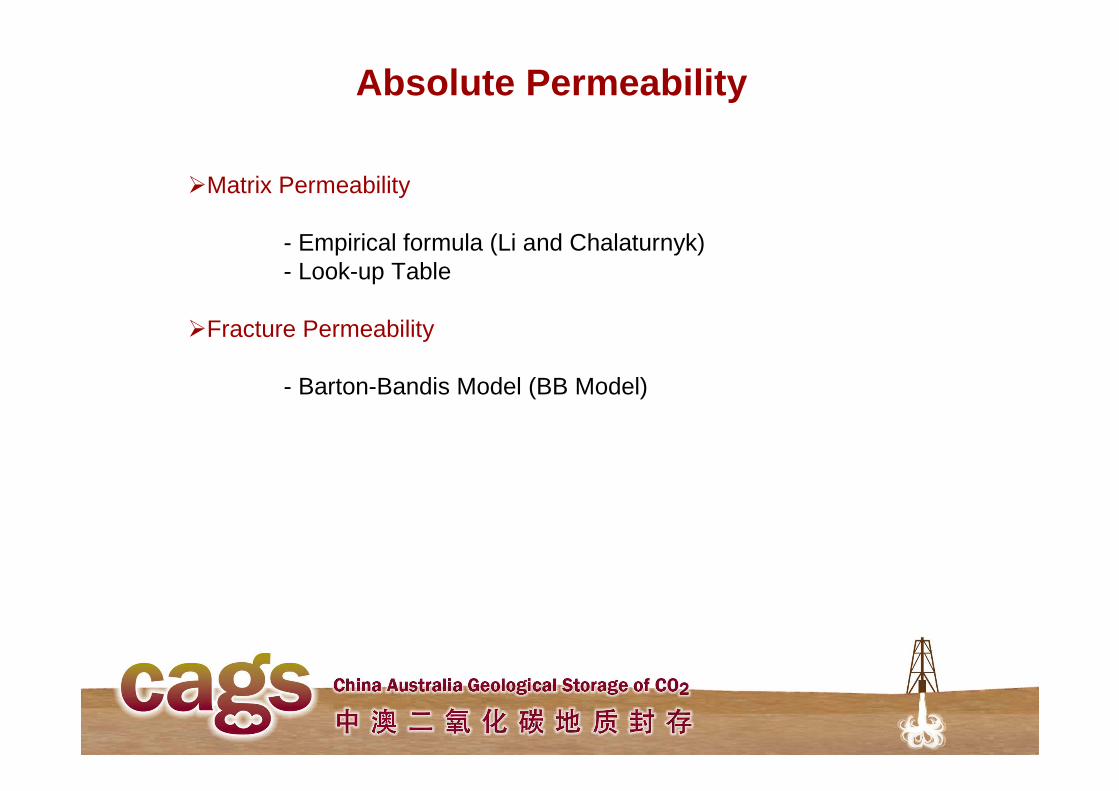
Absolute Permeability

�Matrix Permeability

- Empirical formula (Li and Chalaturnyk)- Look-up Table

�Fracture Permeability

- Barton-Bandis Model (BB Model)

� A secondary fracture system is defined in the grid via dual-permeability

� As pressure increase in the regular grid the stresses are altered, causing the normal stresses on the fractures to increase.

� Eventually the Stress breaks past the Failure Envelope of the rock, causing a fracture to appear (open) and allow fluids to pass through.

Barton -Bandis Model

(CMG, 2009)

Loose Coupling Algorithm

(Susan E. Minkoff et al., 2003)

Geomechanical Simulation Coupled with Compositional S imulator

�Finite element approach:

Two Way Coupling Simulation

n = 0

Reservoir Simulator p, T

Geomechanics Module u, σσσσ, εεεε

n = n+1

n : no of time steps p: pore pressure T: temperature u: displacement σ: stress ε : strain

One Way Coupling Simulation

(CMG, 2009)

Case StudyLeakage Risk of Caprock

�Two-way coupled simulation:

�Grid Dimension: 2m×10m (horizontal)�Grid Number: 500×1×27�Porosity: 0.18�Kv/Kh=1�Sgrm = 0.3�Injection Well: (3, 1, 1) �Perforation Interval: (3, 1, 25) to (3,1, 27)�Injection Rate: 1×104 m3/day (STG surface gas rate)�Injection Period: 2000-1-1 to 2003-1-1�Simulation Period: 2000-1-1 to 2200-1-1

Permeability Model

Results-200yrs Later

Results-200yrs Later

Results-200yrs Later

Results-200yrs Later

Results-200yrs Later

Total Cum Inj, mol = 4.65464E+08CO2 Storage Amounts in Reservoir Moles kg

Gaseous Phase = 0.00000E+00 0.00000E+00Supercritical Phase = 4.09517E+08 1.80228E+07Trapped due to Hysteresis = 1.54067E+08 6.78048E+06Dissolved in Water = 6.79868E+07 2.99210E+06

(CMG, 2009)

Summary

�Coupled numerical simulation of fluid flow and geomechanics is based on the detailed reservoir characterisation of structure, petrophysical property and geomechanical property, ect.

�Coupled simulation can improve our understandings of both movement of CO2 plume and change of geomechanical pattern.

�Besides the effective storage capacity assessment, the coupled simulation can provide the risk information of leakage.