Numerical Simulation of Phytoplankton Productivity in ... · Numerical Simulation of Phytoplankton...

Estuarine, Coastal and Shelf Science (1984) 19,563-589

A

.

Numerical Simulation of Phytoplankton Productivity in Partially Mixed Estuaries

David H. Peterson' and John F. Festa* a U.S. Geological Survey, 345 Middlefield Road, Menlo Park, California 94025 and bNational Oceanic and Atmospheric Administration, Atlantic Oceanographic and Meteorological Laboratories, Physical Oceanography Division, 4301 Rickenbacker Causeway, Miami, Florida 33149, U .S .A .

Received 5 July 1983 and in revised form 30 January 1984

Keywords: plankton distribution; production; light attenuation; estuarine circulation

A two-dimensional steady-state model of light-driven phytoplankton productivity and biomass in partially mixed estuaries has been developed. Effects of variations in river flow, suspended sediment concentration, phytoplankton sinking, self-shading and growth rates on distributions of phytoplankton biomass and productivity are investigated.

Numerical simulation experiments show that biomass and productivity are particularly sensitive to variations in suspended sediment concentrations typical of natural river sources and to variations in loss rates assumed to be realistic but poorly known for real systems. Changes in the loss rate term within the range of empirical error (such as from dark bottle incubation experiments) cause phytoplankton biomass to change by a factor of two. In estuaries with adequate light penetration in the water column, it could be an advantage for phytoplankton to sink. Species that sink increase their concentration and form a phytoplankton maximum in a way similar to the formation of the estuarine turbidity maximum. When attenuation is severe, however, sinking species have more difficulty in maintaining their population.

Introduction

Estuaries represent complex environments in which river and oceanic inputs interact to affect biological and human activities. They serve as a source of freshwater for numerous cities and industries while at the same time are a sink for sewage and other waste material. These waters are typically nutrient rich and are, therefore, ideal environments for high biological productivity. For instance, virtually all of the coastal fisheries species in the Gulf of Mexico have been found to be estuarine-dependent (Texas Department of Water Resources, 1983). During the past few decades, estuarine research has been directed towards understanding the complicated physical and biological processes that act within these waters.

The importance of phytoplankton-based systems to estuarine ecology has long been recognized by biologists and oceanographers (cf., review in Kremer & Nixon, 1978) and perhaps more recently by geochemists. While several factors, biological and physical, may be important to the development and maintenance of phytoplankton communities, physical processes, until recently, have received little attention. It is now acknowledged

563 0272-7714/84/110563+27 $02.00/0 01984 Academic Press Inc. (London) Limited

564 D . H . Peterson &J. F. Festa

that distributional effects due to variations in physical processes must be clarified before variations in a community can be attributed solely to physiological differences.

Recent studies (Perterson et al., 1978; Festa & Hansen, 1978;Rattray & Officer, 1981) have demonstrated the importance of physical processes in explaining some observed geochemical and biochemical phenomena in partially-mixed estuaries. Simple steady- state models show that the formation of a suspended sediment turbidity maximum and observed non-conservative distributions of dissolved silica are coupled to estuarine circulation dynamics. A similar analysis of the importance of physical processes in controlling the production or supply of phytoplankton (organic material), a basic energy source for geochemical phenomena in partially mixed estuaries, has not been reported.

The primary objective of this paper is to examine some effects of estuarine circulation and other environmental factors on phytoplankton development and distributions in partially-mixed estuaries. A simplified two-dimensional, steady-state model of light- driven phytoplankton productivity and biomass in the main channel of a river-estuarine system is developed. Steady-state circulation and suspended sediment models (Festa & Hansen, 1976; 1978) are extended to include photosynthetic carbon assimilation by phytoplankton. Effects of variations in river flow, suspended sediment concentration, phytoplankton sinking, self-shading and growth rates on steady-state distributions of phytoplankton biomass and productivity are investigated.

Numerical oceanic models of phytoplankton development, which have been applied to Puget Sound (Winter et al., 1975), Narragansett Bay (Kremer & Nixon, 1978) and elsewhere, serve as an excellent frame of reference for this study. Phytoplankton contributions from shoals to adjacent main channels are believed to be important (Cloern & Cheng, 1981), but are not considered herein. Effects of nutrient availability and temperature are also neglected.

Careful field studies are essential to better define phytoplankton structure and development in relation to estuarine circulation and river flow (Tyler & Seliger, 1978). In situ experiments in northern San Francisco Bay (Peterson et al., 1985a, b; Cole & Herndon, 1979), of 12- and 24-h average phytoplankton productivity in relation to depth variations in light intensity provide information on phytoplankton productivity and are, therefore, used as a guide in selecting various model parameters.

Factors affecting phytoplankton development

Circulation and light are the factors herein considered to be of fundamental importance for understanding the complex ecological systems in most estuaries. Water circulation influences phytoplankton development by affecting rates of supply, removal, and dilution of phytoplankton; whereas light drives the photosynthetic activity essential for that development. Others factors such as phytoplankton sinking, self-shading and net growth rates are also included. Effects of nutrient availability and water temperature, often considered to be important in coastal environments, are neglected for reasons described below.

?

b

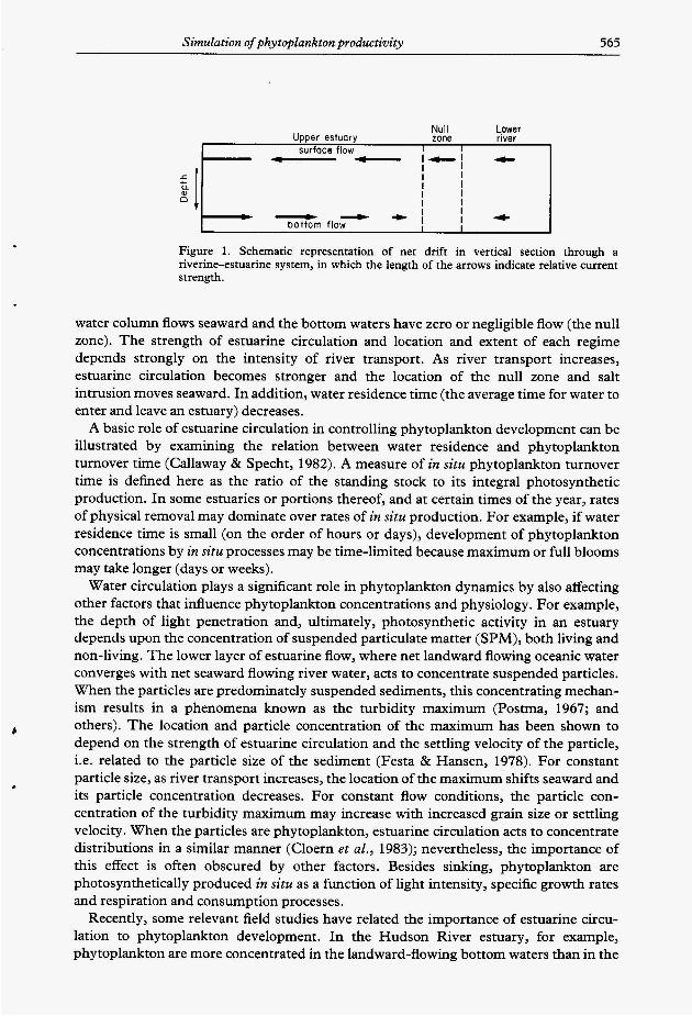
Water circulation The mean or tidally-averaged circulation in partially mixed estuaries is characterized by three distinct flow regimes (Figure 1): an upstream regime where the flow is seaward at all depths, a downstream regime where the flow is seaward in the upper water column and landward in the lower water column, and a transitional regime where the upper

Simulation of phytoplankton productivity 565

I

,

surface flow 1 I - 1 - 1 4- I I

x II I

I I I

! I I

Figure 1. Schematic representation of net drift in vertical section through a riverine-estuarine system, in which the length of the arrows indicate relative current strength.

water column flows seaward and the bottom waters have zero or negligible flow (the null zone). The strength of estuarine circulation and location and extent of each regime depends strongly on the intensity of river transport. As river transport increases, estuarine circulation becomes stronger and the location of the null zone and salt intrusion moves seaward. In addition, water residence time (the average time for water to enter and leave an estuary) decreases.

A basic role of estuarine circulation in controlling phytoplankton development can be illustrated by examining the relation between water residence and phytoplankton turnover time (Callaway & Specht, 1982). A measure of in situ phytoplankton turnover time is defined here as the ratio of the standing stock to its integral photosynthetic production. In some estuaries or portions thereof, and at certain times of the year, rates of physical removal may dominate over rates of in situ production. For example, if water residence time is small (on the order of hours or days), development of phytoplankton concentrations by in situ processes may be time-limited because maximum or full blooms may take longer (days or weeks).

Water circulation plays a significant role in phytoplankton dynamics by also affecting other factors that influence phytoplankton concentrations and physiology. For example, the depth of light penetration and, ultimately, photosynthetic activity in an estuary depends upon the concentration of suspended particulate matter (SPM), both living and non-living. The lower layer of estuarine flow, where net landward flowing oceanic water converges with net seaward flowing river water, acts to concentrate suspended particles. When the particles are predominately suspended sediments, this concentrating mechanism results in a phenomena known as the turbidity maximum (Postma, 1967; and others). The location and particle concentration of the maximum has been shown to depend on the strength of estuarine circulation and the settling velocity of the particle, i.e. related to the particle size of the sediment (Festa & Hansen, 1978). For constant particle size, as river transport increases, the location of the maximum shifts seaward and its particle concentration decreases. For constant flow conditions, the particle concentration of the turbidity maximum may increase with increased grain size or settling velocity. When the particles are phytoplankton, estuarine circulation acts to concentrate distributions in a similar manner (Cloern et al., 1983); nevertheless, the importance of this effect is often obscured by other factors. Besides sinking, phytoplankton are photosynthetically produced in situ as a function of light intensity, specific growth rates and respiration and consumption processes.

Recently, some relevant field studies have related the importance of estuarine circulation to phytoplankton development. In the Hudson River estuary, for example, phytoplankton are more concentrated in the landward-flowing bottom waters than in the

566 D. H . Peterson G. J. F. Festa

seaward-flowing surface waters (Malone, 1977; Malone et al., 1980). Water residence time for certain river flow conditions is short, on the order of six days, and is insufficient for complete in situ phytoplankton utilization of the enormous New York City waste- derived nutrient source. As a result, a major portion of these nutrients are carried beyond the mouth of the Hudson to coastal shelf waters. An unknown fraction of these waste- derived nutrients doubtless returns to the estuary, perhaps in the form of phytoplankton. The relation between physical processes and phytoplankton distributions have also been clearly shown for the Chesapeake Bay (Tyler & Seliger, 1978), and its tributary Potomac River estuary (Tyler et al., 1982). Even in San Francisco Bay, a geometrically complex estuary with more intense vertical mixing than Chesapeake Bay, a variety of phytoplankton-related studies have also identified, or inferred, the importance of seasonal and spatial variations in estuarine water circulation to phytoplankton development (Cloern et al., 1983).

Light The growth and development of phytoplankton ultimately depends upon the distribution of the light field in estuarine waters (cf. Hitchcock & Smayda, 1977). The amount of light transmitted in wavelengths of photosynthetically active radiation, PAR, approximately 400-700 nm, is affected by atmospheric attenuation, water surface reflection and water-column attenuation. Factors determining and influencing temporal and spatial variations in light arriving at the water surface are, in general, well documented (Smith & Morgan, 1981; and other authors). A portion of the solar and sky radiation incident upon a water surface is reflected depending on such factors as sun angle, degree of overcast and roughness of the water surface (Cox & Munk, 1956). The penetration and distribution of underwater radiant energy which is not reflected is primarily determined by absorption and to a lesser extent by scattering phenomena (Jerlov, 1976, 1977). The effects of light reduction at or above the water surface is beyond the scope of this simple steady-state model study. The major emphasis will be on the effects of light attenuation in the water column (Hojerslev, 1978); the supply of radiant energy at the water surface available for photosynthetic activity is, therefore, assumed constant. Light attenuation by the water itself is considered negligible [e.g., 0.04 m- ' for A= 400 to 600 nm and 0.14 m- ' for 300 to 700 nm (Smith & Baker, 198l)l.

In estuaries, the decrease in light intensity with increasing water depth is predominately due to absorption of light by suspended particulate matter. As concentra-

increase at the expense of the photic depth. Thus, the effect of water-column light intensity on phytoplankton is complicated by the large spatial variations in concentrations of suspended sediment. As previously discussed, circulation dynamics plays an important role in determining these distributions and in turn, the horizontal and vertical distribution of light. Phytoplankton distributions also directly affect the amount of light present in the water column. Like sediment, they too absorb light and limit their own development by a negative feedback process referred to as self-shading.

A decrease in water transparency due to the presence of suspended material is commonly observed in estuaries. Examples of severe light attenuation due to extremely high river-borne concentrations of suspended material have been reported near the mouth of the Seine (Romana, 1979) and Amazon (Edmond et al., 1982) rivers. There, the major phytoplankton blooms are prohibited from appearing until after concentrations of suspended material are reduced by sinking and dilution with seawater.

tions of suspended particles, including phytoplankton, increase, the aphotic depth will 4

%


Nutrient availability Plant nutrients, which fertilize plant growth, are supplied from both natural and anthropogenic sources. These nutrients may be introduced to the system over a large area, such as through the atmosphere, or may enter at a fixed point, such as through a waste outfall. The availability of nutrients provides a control on the upper limit of phytoplankton biomass and possibly plays a role in altering community species.

Estuaries are rich in nutrients relative to levels observed in the ocean (Redfield et al., 1963) and eutrophic lakes (Schindler, 1977; Schelske, 1979). Concentrations of nitrogen and phosphorous, for example, required for nutrient limitations are relatively low when compared to those commonly reported values for urbanized estuaries including the Hudson (Simpson et al., 1977), Delaware (Sharp et al., 1982), and Potomac River estuaries (Callender & Hammond, 1982) and San Francisco Bay (Conomos et al., 1979). For this and other reasons (cf. Goldman et al., 1979), nutrient concentrations are at or near saturation levels in many estuaries. Nutrient availability is, therefore, considered to be of secondary importance.

Water temperature Water temperature varies in response to seasonal climate and to the temperature of the estuarine source waters. The most significant effect of temperature on phytoplankton development is thought to occur at water temperatures generally below 10" C where phytoplankton growth could decrease and certain species could be eliminated (Fogg, 1965). Because water temperatures are generally above than 10" C in most mid-latitude estuaries during most of the year, neglecting temperature effects seems reasonable except during the mid winter season (cf. Malone, 1982; Tyler & Seliger, 1981). Winter conditions are, therefore, not considered in this study.

Model development

Development of a light-driven phytoplankton model involves determination of the circulation field, determination of the suspended sediment field, and incorporation of both these fields and other factors into a model of particulate organic carbon. The circulation and suspended sediment fields are obtained by using the steady-state models of Festa and Hansen (1976; 1978). Modifications have been made to allow for effects of variable width.

Circulation The problem considered is that of a steady-state, two-dimensional laterally homo- geneous estuary. The coordinate system is Cartesian in x and z, where x increases toward the river and z is positive upwards. A linear equation of state, p =po( 1 +PS), is assumed, and the Boussinesq approximation employed.

The horizontal and vertical momentum balances, continuity of flow, and conservation of salinity are:

U,+(uIJ),+(uWz= -Pol~P,+(A,bu,),+(A,bu,),, (la)

568 D. H . Peterson & J . F. Festa

where U=ub, W=wb, p=p’-j; pgdz, u and w are the horizontal and vertical components of velocity, respectively, b is the channel width, p’ is the hydrostatically reduced pressure, S is the salinity field, po is the density of freshwater, /? is the coefficient of ‘salt contraction’, A,, A, and K,, K, are the horizontal and vertical exchange coefficients of momentum and salt, respectively, and g is the gravitational acceleration.

Although tidal fluctuations have been averaged out, the tidal currents are considered to be the primary source for turbulent mixing. For simplicity, the exchange coefficients, a measure of the tidal current strength, and the depth of the estuary, H, are chosen to be constant. The channel width, b, is chosen to be a smoothly varying function of x , such that,

b=b,+(b,-b,) (1 -tanh ( C X ) } , (le)

where b, and b, represent the widths at the river and ocean boundary, respectively. Equations (la), (1 b), and (lc) are used to write a vorticity equation in terms of a stream

function, w where U = - y2 and W= ty,. The vorticity equation and salt equation, (Id), are iterated numerically to a steady-state, subject to the following boundary conditions. At the river boundary, zero salinity and a parabolic velocity profile having a transport T, = U,b,H, where U, is the vertically-averaged river flow, are specified. At the seaward boundary, bottom salinity is specified and horizontal diffusive fluxes of salt and vorticity are assumed constant, but unspecified. A zero vertical flux of salt is required at a no-slip bottom and free-slip surface boundary.

Suspended sediment The suspended sediment model is consistent with the circulation model; the same exchange coefficients are used for sediments as for salinity, and advection is by currents derived from the circulation model. Consideration is limited to conditions in which sediment concentrations have a negligible effect on water density.

The equation governing the distribution of suspended sediment is:

where C* is the concentration of suspended sediment, w* is the settling velocity of the sediments and all other parameters are as previously described. The settling velocity is considered to be constant; therefore, specifying w* is approximately equivalent to specifying the particle diameter of the sediment to be modelled.

The sediment equation is solved subject to the following boundary conditions. At the river end, the bottom sediment concentration is specified and an exponential vertical profile is maintained. At the seaward boundary, the horizontal diffusive flux of sediment is unspecified but required to be horizontally non-divergent, and a bottom sediment source is maintained. Zero total vertical flux of sediment is required at both the bottom and surface boundaries; that is, zero net deposition or erosion of bottom sediments and sediment conservation at the surface is assumed.

L

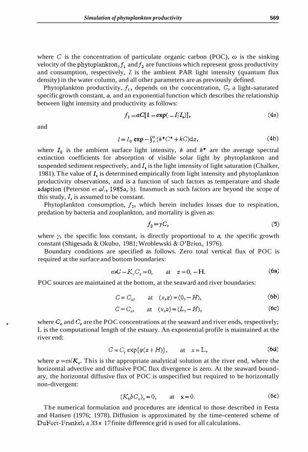
Particulate organic carbon The equation used for modelling phytoplankton or, equivalently, particulate organic carbon is:

(b~)~+(~~),+(W~),+(~b~),=(~,b~,),+(~,b~,),+bdf,[~,~,C*]-f~[~]}, (3)


where C is the concentration of particulate organic carbon (POC), o is the sinking velocity of the phytoplankton,f, and fz are functions which represent gross productivity and consumption, respectively, Z is the ambient PAR light intensity (quantum flux density) in the water column, and all other parameters are as previously defined.

Phytoplankton productivity, f,, depends on the concentration, C, a light-saturated specific growth constant, a, and an exponential function which describes the relationship between light intensity and productivity as follows:

(44 fl = aCP - exp( - U4)ly and

I=Z, exp-j; (K*C*+kC)dz, (4b)

where I, is the ambient surface light intensity, K and K* are the average spectral extinction coefficients for absorption of visible solar light by phytoplankton and suspended sediment respectively, and 1, is the light intensity of light saturation (Chalker, 1981). The value of I, is determined empirically from light intensity and phytoplankton productivity observations, and is a function of such factors as temperature and shade adaption (Peterson et al., 1985a, b). Inasmuch as such factors are beyond the scope of this study, Zs is assumed to be constant.

Phytoplankton consumption, fz, which herein includes losses due to respiration, predation by bacteria and zooplankton, and mortality is given as:

f 2 = G (5)

where y, the specific loss constant, is directly proportional to a, the specific growth constant (Shigesada & Okubo, 1981; Wroblewski & O’Brien, 1976).

Boundary conditions are specified as follows. Zero total vertical flux of POC is required at the surface and bottom boundaries:

WC - KvCz = 0, at z = 0, - H. (64

POC sources are maintained at the bottom, at the seaward and river boundaries:

C=C,, at (x,z)=(O,-H), (6b)

C=C,, at (x,z)=(L,-H), (6c)

where C, and C, are the POC concentrations at the seaward and river ends, respectively; c

L is the computational length of the estuary. An exponential profile is maintained at the river end:

C=C,exp{p(z+H)}, at x=L , ( 6 4

where p = o/KV. This is the appropriate analytical solution at the river end, where the horizontal advective and diffusive POC flux divergence is zero. At the seaward boundary, the horizontal diffusive flux of POC is unspecified but required to be horizontally non-divergent:

(K,bC,),=O, at x=O. (6e)

The numerical formulation and procedures are identical to those described in Festa and Hansen (1976; 1978). Diffusion is approximated by the time-centered scheme of DuFort-Frankel; a 33 x 17 finite difference grid is used for all calculations.

570 D. H. Peterson Q J. F . Festa

Model calculations

This model has been developed to help understand the basic processes which influence the distribution of phytoplankton in partially mixed estuaries. Qualitatively, the results presented here will behave similarly for a range of estuarine dynamics; quantitatively, they will depend critically on the choice of parameters.

Circulation and suspended sediment distribution Circulation fields are obtained for depth-averaged river flows ranging from 0.8 to 4 cm s- ', depth, H, of 10 m and length, L, of 120 km. A horizontal salinity difference, AS, of 27%0 is maintained between the seaward and river boundaries. A complete listing of the model parameters for both circulation and suspended sediments is presented in Table 1. The mixing coefficients are considered typical of estuaries with moderate to high tidal mixing, such as San Francisco Bay. Suspended sediment fields are calculated for sediment having a settling velocity, w*, of -6 x cm s-' and a river source, C,*, having a range of 0 to 50 mg I-'; the ocean source, C,* is considered to be 115 of the river source.

Distributions of salinity, velocity, and suspended sediments (Figure 2) show the typical pattern of seaward flow of the surface waters and landward flow of the deeper waters, salt intrusion, and presence of a turbidity maximum. As the river flow increases, there is an increase in both stratification and strength of the estuarine circulation, salt intrusion is weakened, and the turbidity maximum moves seaward and decreases in magnitude.

Particulate organic carbon distributions

Steady state POC distributions are obtained for a river source, C,, of 25 pg at 1-' and an ocean source, Coy of 5 pg at I-'. The organic carbon to chlorophyll ratio is considered to be 40 to 1. Typical values of the parameters used for the model runs are as follows. The specific growth constant, a, is 0.5 d - ' and the specific loss constant, y, is 5% of a. The average spectral extinction coefficient for sediment, k*, is 0.1 m-' (mg 1-')-I and for POC, k, is 0.006m-' (pg at I-')-'. The value I,/I,, a measure of the surface light intensity, is 12 and the phytoplankton sinking velocity, w, is -4 m d-'. The range over which these parameters are varied is listed in Table 1; these values are consistent with observations in partially mixed estuaries (see appendix).

4

TABLE 1 . Model parameters

Circulation and suspended sediment model

U,=(0.8, 1 ,2 ,4)cms-' p=7.57 (%)-I H= 10 m g = 9 8 0 c m ~ - ~ L= 120 km ns, = 27% b0=5km ~ , = 6 c m ~ s - ' b , = l k m K,=2 x lo6 cm2 s-' (=ax 10-5km-' A,= 10cmz s-'

Particulate organic carbon model

Cr=25pgat1-' ~ = ( 5 % , 10%) a k*=o.l m - l (mgl-')-I Co=5pgat1-' carbon/chlorophyll ratio = 4011 w = - ( 0 , 2 , 4 , 6 , 8 ) m d - ' a=(0.5, 1.0) d-' k=(0.6,5.4,6.0, 6.6) x m-' (pg at I - ' ) - ' Z,,/Z,= 1.2,6,9, 12

Simulation of phytoplankton productivity 57 1

,

River flow I crn s-' R i v e r flow 4 cm s-' Salinity ( S )

Stream function ( $ 1

Horizontal velocity ( 0 )

Vertical velocity (4

Suspended sediments (C*)

0 30 60 90 120 0 30 60 90 I20

Distance (km)

Figure 2. Salinity, stream function, horizontal velocity and vertical velocity fields for the case of U, = 1 and 4 cm s- l , H= 10 m and L = 120 km. Salinity is scaled by ASh=27K, stream function by 100 m3 s- l and w by cm s-'. Velocity fields are contoured in cm s- '.

Injluence of light Light intensity in the riverine/estuarine environment depends on light availability at the water surface, I , , and on light extinction due to particles (phytoplankton C, and suspended sediment, C*) in the water. To better understand the influence of light on phytoplankton distribution, numerical simulations are made for two distinct estuarine environments, one which is free of suspended sediments and the other for which varying degrees of suspended sediments are present in the water column.

572 D. H . Peterson &J. F. Festa

River flow I cm s-I River flow 4 crn s- '

Distance (krn)

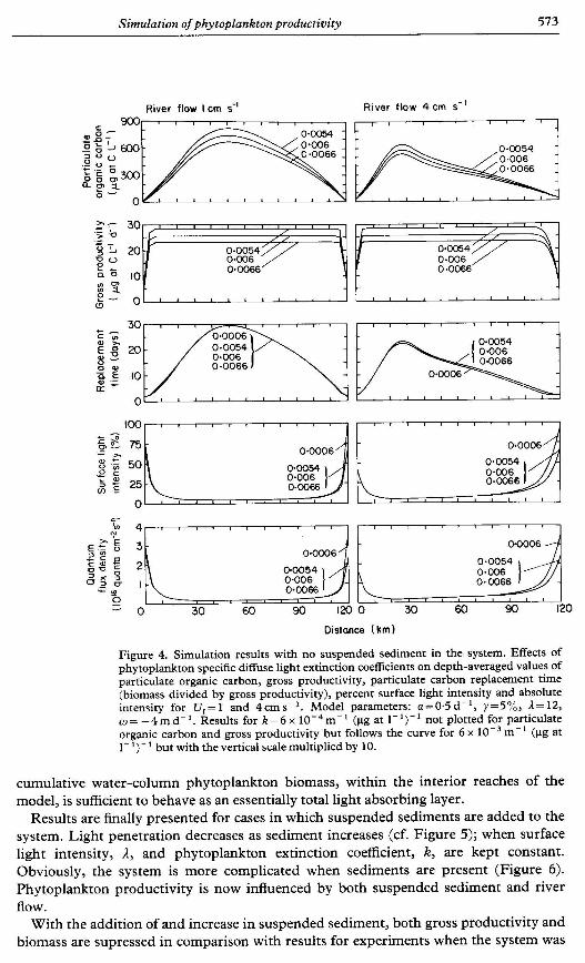
Figure 3. Simulation results with no suspended sediment in the system. Effects of surface light intensity 1 (where 1 = Io/ZJ on depth-averaged values of particulate organic carbon (phytoplankton biomass), gross productivity, percent surface light intensity and absolute intensity for U, = 1 and 4 cm s- '. Model parameters: a = 0.5 d- ', y = 5 % , k = 6 x m-' (pgat l- ')-' ,m= -4md- ' .

Results are initially presented for a model in which only the surface light intensity, I,, is varied. The suspended particle concentration is set equal to zero and k and I , are constant. Variations in surface light intensity are therefore modelled by the dimensionless parameter A=Zo/Zs; il is varied between 1.2 and 12.0. The results, as expected, indicate that cumulative biomass and gross productivity per unit area decrease with decreasing il (Figure 3) and the quantum flux density (i.e., the average water-column light intensity) also decreases. The value of the average water-column light intensity relative to surface light intensity increases (Figure 3) .

Results are next presented for simulations where only the degree of self-shading (i.e., the phytoplankton extinction coefficient, k ) is varied. Once again, there is no suspended sediment in the water, and the surface light intensity is kept constant at a high light condition, A = 12. As might be anticipated, when K decreases both cumulative biomass and gross productivity per unit area increase (Figure 4). The average water-column biomass replacement time and light intensity is not affected (Figure 4).

One of the more important results of these simple calculations is that when there is no suspended sediment in the system, the gross phytoplankton productivity per unit area is constant and independent of river flow (Figures 3 and 4). This happens because the


Rwer flow I cm s'l River flow 4cm s-'

Distance (km)

Figure 4. Simulation results with no suspended sediment in the system. Effects of phytoplankton specific diffuse light extinction coefficients on depth-averaged values of particulate organic carbon, gross productivity, particulate carbon replacement time (biomass divided by gross productivity), percent surface light intensity and absolute intensity for U,= 1 and 4cms-'. Model parameters: a=O.5 d-', y=5%, 1= 12, w = -4 m d-'. Results for k = 6 x m- ' (pg at 1- ')-' not plotted for particulate organic carbon and gross productivity but follows the curve for 6 x m- ' ()rg at 1- ')- ' but with the vertical scale multiplied by 10.

cumulative water-column phytoplankton biomass, within the interior reaches of the model, is sufficient to behave as an essentially total light absorbing layer.

Results are finally presented for cases in which suspended sediments are added to the system. Light penetration decreases as sediment increases (cf. Figure 5); when surface light intensity, I, and phytoplankton extinction coefficient, k, are kept constant. Obviously, the system is more complicated when sediments are present (Figure 6) . Phytoplankton productivity is now influenced by both suspended sediment and river flow.

With the addition of and increase in suspended sediment, both gross productivity and biomass are supressed in comparison with results for experiments when the system was

574 D. H . Peterson 9-7, F. Festa

River f low I cm s-'

01 i I 1 I I ' ' ' I '

iQ 0 - lLi, iJ 11 h

0 30 60 90 120

River f low 4 cm s-'

7

Distance ( k m )

Figure 5. Simulation results with no phytoplankton in the system. Effects of suspended sediment concentrations on depth-averaged values of percent surface light intensity and absolute intensity for U,= 1 and 4cms-' . Model parameters: High C,* =50 mg I-', Low C,*=25 mg I-' , A= 12, o= -4 m d-'.

devoid of suspended sediment. This is similar to but not the same as the response with increasing specific diffuse light extinction coefficients for phytoplankton (Figure 4). When suspended sediment is present, phytoplankton productivity is sensitive to increasing river flow because phytoplankton are competing with suspended sediment for light. The competition is less favorable for phytoplankton at higher river flows because in this model suspended sediment concentrations in the estuary are largely controlled by the river suspended sediment concentration (Figure 5) whereas phytoplankton biomass is largely controlled by growth (i.e., Figures 3 and 4). An increasing fraction of phytoplankton are swept away at higher flows but river-borne suspended sediment concentrations are relatively constant. The result is a decreasing proportion of phytoplankton to


River f low I cm s-' River f low 4 c m s-'

7

. _ - W

0 30 60 90 1200 30 60 90 120

Distance (krn)

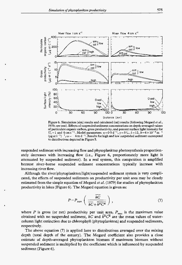
Figure 6. Simulation (sim) results and calculated (cal) results (following Megard et al., 1979; see text). Effects of suspended sediment concentrations on depth-averaged values of particulate organic carbon, gross productivity, and percent surface light intensity for V,=1 and4cms-'. Modelparameters: a=0,5d-' ,y=5%, I = 1 2 , k = 6 ~ 1 O - ~ m - ' (pg at 1- ')- ', w = -4 m d- '. Results for high and low suspended sediment correspond to distributions depicted in Figure 5.

suspended sediment with increasing flow and phytoplankton photosynthesis proportionately decreases with increasing flow (i.e., Figure 6, proportionately more light is attenuated by suspended sediment). In a real system, this competition is amplified because river-borne suspended sediment concentrations typically increase with increasing river flow.

Although the river/phytoplankton/light/suspended sediment system is very complicated, the effects of suspended sediments on productivity per unit area may be closely estimated from the simple equation of Megard et al. (1979) for studies of phytoplankton productivity in lakes (Figure 6). The Megard equation is given as:

kC

kC+ k*C*

where P is gross (or net) productivity per unit - area, P,,, is the maximum value obtained with no suspended sediment, kC and k*C* are the mean values of water- column light extinction due to chlorophyll (phytoplankton) and suspended sediments, respectively.

The above equation (7) is applied here to distributions averaged over the mixing depth (total depth of the estuary). The Megard coefficient also provides a close estimate of depth-averaged phytoplankton biomass if maximum biomass without suspended sediment is multiplied by the coefficient which is influenced by suspended sediment (Figure 6).

576 D. H . Peterson & J. F. Festa

River flow I crn s-'

Figure 7. Simulation results for effects of maximum specific growth rate on depth- averaged values of particulate organic carbon and gross product using for U,= 1 and 4cm s-I . Model parameters: High Cr*=50mg 1-', Low C,* =25 mg 1-', y =5%, , l=12,k=6x 10 -3m- ' (pgatl-')- ' ,w= - 4 m d - ' .

Influence of growth Specific growth rate, a, is the phytoplankton productivity per unit biomass. In con- sidering combinations of variable maximum growth rate, suspended sediment and river flow, the distributions, as expected, have many variations. Without suspended sediment, depth averaged gross productivity is twice as high for a maximum growth rate of 1 d- ' as 0.5 d-l . With the addition of suspended sediment, or when phytoplankton are competing with suspended particulate matter for light, the depth averaged gross productivity is generally more than two times higher for a maximum growth rate of 1 d- ' compared with 0.5 d-'. Thus, when a increases, there is a corresponding or greater increase in the water-column average growth rates, but C is relatively unchanged (Figure 7). This occurs because the equations as written describe collective losses, y, as a constant fraction of a and not biomass (i.e., analogous to an income tax rather than a property tax) (Angus &Wilson, 1976).

Influence of consumptive rates Phytoplankton biomass is very sensitive to changes in consumptive rates (Figure 8). This is especially important because the values of collective losses in natural systems are poorly known (Kalff & Knoechel, 1978; Shigesada & Okubo, 1981). For example, phytoplankton 'respiration' rates are estimated at less than 5% of maximum productivity (Malone & Neale, 1981), but with a 'f 100% error (Malone & Neale, 1981; Platt & Jassby, 1976). In view of our present state of knowledge, we conclude that a very simple model of consumptive rates is adequate if not preferable.

Influence of sinking At low river flow (e.g., U, = 1 cm s- ') phytoplankton concentrations are enhanced by the estuarine mechanism in systems with high phytoplankton sinking rates and with a relatively high light intensity (e.g., with a low concentration of suspended sediments,


R ~ v e r flow I cm s-' River flow 4 c m s- '

Distance ( k m )

Figure 8. Simulation results for effects of specific loss rate on depth-averaged values of particulate organic carbon, gross productivity, percent surface light intensity and net productivity for U,= 1 and 4 cm sC'. Model parameters: a=0.5 d - ', 1= 12, k = 6 x 1 0 3 m - ' (pgat I-')- ' ,w= -4md- ' .

Figure 9, upper panel). However, when available light is decreased (e.g., the concentration of suspended sediments is increased) this mechanism may become disadvantageous and non-sinking forms may attain higher concentrations than sinking forms (Figure 9). At high river flow non-sinking forms attain higher concentrations than sinking forms with or without suspended sediment (Figure 9, lower panel).

Overview T o gain a greater understanding of estuarine systems a variety of techniques including field, laboratory and modelling efforts are necessary (cf. Nixon et al., 1979). In this section we attempt to relate some of the numerical results to observations. The implications from the results of the numerical simulations are prefaced with a reminder that while many of the simplifying assumptions in numerical simulation models may seem rather severe, the assumptions in obtaining some of the field observations (e.g., incubation experiments) can be no less severe.

Light is sharply attenuated in the riverine/estuarine environment by high concentrations of suspended particulate matter including inorganic particles and living phytoplankton. Perhaps the clearest finding with regard to field observations is that

578 D. H . Peterson &J. F. Festa

Suspended sediment: river flow I cm s-' High

OpBl .

15

5

-5 0 30 60 90 1200 30 60 90 1200 30 60 90 120

Distance (km)

Low

Suspended sediment: river f low 4 cm s - '

Intermediate

7 0 8

-/

High

L

- 0 30 60 90 120

Distance ( k m

Figure 9. Simulation results for effects of sinking on depth-averaged values of particulate organic carbon, gross productivity and net productivity for U, = 1 (upper panel) and 4 cm s- ' (lower panel). Model parameters: a=0.5 d- ', y= 5%, I = 12, k = 6 x (pg at l-')-' . High (C*=50mg1-'), Intermediate (C,*=33,3mgl-'), Low a

( c*=25 mg I-').

phytoplankton productivity and biomass are strongly suppressed by increasing concentrations of suspended sediments in the approximate range of 10 to 100 mg 1-' (see also Wofsy, 1983). Effects of suspended sediment on phytoplankton biomass and productivity even below concentrations of 10 mg 1- ' have been identified for relatively clear coastal ocean water (Smith, 1982). This seems especially relevant because the concentration of suspended sediments in rivers is typically within this range or higher (Milliman & Meade, 1983, and references cited). Results from the numerical simulations


TABLE 2. Estuarine examples of suspended sediment concentrations and phytoplankton productivity (PP) in the region of the turbidity maximum (TM) and outer estuary (OE)

Estuary OE TM OE TM References

Delaware <20 40-70 640 230 Sharp et al. (1982), Biggs et al. (1983), Sharp & Pennock, personal communication (1982)

San Francisco Bay < 20 > 50 360 270 Cole (1982), Peterson et al. (1985a, b) Seine <20 100-600 -1000‘ < 50a Romana (1979) Tamar 1 2 0 >200 ?b ?b Morris et al. (1982) Bristol Channel < 20 > 75 450 20 Joint & Pomroy (1981) Gironde <20 >loo0 > 100’ < 50” Romana (1982)

“Estimated for upper meter. bPhotosynthetic removal of plant nutrients appears not to be important relative to mixing river water and seawater in this estuary (Morris et al., 1981).

usually agree with the distribution of phytoplankton productivity and biomass observed in estuaries with high concentrations of suspended sediments (Table 2). Because the formulation of Megard et al. (1979) describes the general effects of suspended sediments on phytoplankton productivity in the numerical simulation model, their equation may provide a useful frame of reference for analysis of real systems.

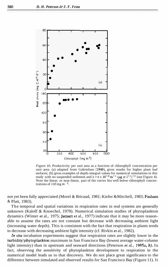
The suspended sediment particles discussed above reduce the availability of surface light for phytoplankton growth. Living phytoplankton also attenuate light primarily by absorption, in effect a self-shading mechanism. Field studies in Chesapeake Bay clearly indicate this mechanism is an important feature of estuarine phytoplankton development (Seliger et al., 1975, figure 10, p. 199; see also Wofsy, 1983). The importance of self- shading is also obvious in numerical models of phytoplankton growth because unrealisti- cally high values result when such effects are neglected (Shigesada & Okubo, 1981, and others cited therein). Although the details of the mechanism are complex (Fushansky, 1981), it serves our purposes here to ‘isolate’ self-shading effects by simulations without sediments.

Cumulative phytoplankton biomass per unit area is constant when the one- dimensional steady-state equation of self-shading with variable phytoplankton settling velocity is solved analytically (Shigesada & Okubo, 1981, figure 4, p. 322). The estuarine model produced somewhat similar results. The difference is that longitudinal as well as vertical processes influence cumulative phytoplankton biomass while cumulative productivity per unit area remains constant. Interestingly, this result has been demonstrated empirically for higher plants (Gabrielsen, 1948; also discussed in Bjorkman, 1981), where productivity approaches a constant value as the concentration of leaf chlorophyll (instead of phytoplankton chlorophyll) per unit leaf area increases (Figure 10, adapted from Gabrielsen, 1948; also note Figure 4, the simulated response with different values of k ) . As k increases in the estuarine model, both cumulative biomass (Talling, 1981; Takahashi & Parsons, 1972; Parsons et al., 1977, table 2, p. 104), and, within the assumptions in the model, productivity decreases because it takes less biomass to ‘soak up’ the same amount of light. In real systems the potential effects of variations in k has

580 D. H. Peterson & J . F. Festa

Figure 10. Productivity per unit area as a function of chlorophyll concentration per unit area: (a) adapted from Gabrielsen (1946), gives results for higher plant leaf surfaces; (b) gives examples of depth-integral values for numerical simulations in this study with no suspended sediment and k =6 x m-' (pg at I-')-' (see Figure 4). Note the linear, or near-linear, part of the curves lies well below chlorophyll concentrations of 100 mg m-*.

$ 140 Z - U

120- a

I 0 0

8 0

6 0 -

4 0

20,

not yet been fully appreciated (Morel & Bricaud, 1981; Kiefer &Mitchell, 1983; Fasham & Platt, 1983).

The temporal and spatial variations in respiration rates in real systems are generally unknown (Kaloff & Knoechel, 1978). Numerical simulation studies of phytoplankton dynamics (Winter et al., 1975; Jamart et al., 1977) indicate that it may be more reasonable to assume the rates are not constant but decrease with decreasing ambient light (increasing water depth). This is consistent with the fact that respiration in plants tends to decrease with decreasing ambient light intensity (cf. Rivkin et al., 1982).

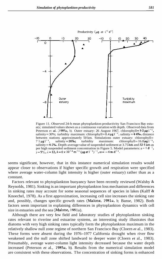
In situ incubation experiments suggest that respiration rates are slightly lower in the turbidity/phytoplankton maximum in San Francisco Bay (lowest average water-column light intensity) than in upstream and seaward directions (Peterson et al., 1985a, b) . In fact, observing the sensitivity of phytoplankton development to respiration in the numerical model leads us to that discovery. We do not place great significance to the difference between simulated and observed results for San Francisco Bay (Figure 11). It

I I I I ..... -

- -

- -

-

-* - ( b )

I I I I . 0 2 0 0 4 0 0 6 0 0 8 0 0 1000

Chlorophyll (mg m-')


Productivity (pg at l-' d-'1

Figure 11. Observed 24-h mean phytoplankton productivity San Francisco Bay estuary; simulated values shown as a continuous variation with depth. Observed data from Peterson et a2. (1985a, b). Outer estuary: 26 August 1967, chlorophyll =3.2 pg 1-', salinity = 30%; turbidity maximum: chlorophyll = 8.4 pg 1- ', salinity = 4.4%0, distance between stations approximately 50 km. Simulations outer estuary: chlorophyll = 7 1 g 1 salinity =26%; turbidity maximum: chlorophyll = 16.8 pg I-', salinity = 4.2%. Depth-average value of suspended sediment at 3.75 km and 52.5 km as per high suspended sediment concentration in Figure 5. Model parameters: a = 1 d-', y=5%,1=12,k=6x 10-3m-1 (pgatl-')-',w= -4md- ' .

seems significant, however, that in this instance numerical simulation results would appear closer to observations if higher specific growth and respiration were specified where average water-column light intensity is higher (outer estuary) rather than as a constant.

Factors relevant to phytoplankton buoyancy have been recently reviewed (Walsby & Reynolds, 1981). Sinking is an important phytoplankton loss mechanism and differences in sinking rates may account for some seasonal sequences of species in lakes (Kalff & Knoechel, 1978). As a first approximation, increasing cell size increases the sinking rate and, possibly, changes specific growth rates (Malone, 1981a, b; Banse, 1982). Both factors seem important in explaining differences in phytoplankton dynamics with cell size in estuaries and the sea (Malone, 198 1 a).

Although there are very few field and laboratory studies of phytoplankton sinking rates relevant to riverine and estuarine systems, an interesting study illustrates that diatoms with very high sinking rates typically form the phytoplankton maximum in the relatively shallow null zone regime of northern San Francisco Bay (Cloern e t al., 1983). These forms were absent during the 1976-1977 California drought when river flow weakened and the null zone shifted landward to deeper water (Cloern e t al., 1983). Presumably, average water-column light intensity decreased because the water depth increased (Peterson e t al., 1985a, b). Results from the numerical simulation model are consistent with these observations. The concentration of sinking forms is enhanced

582 D. H. Peterson &J. F. Festa

relative to non-sinking forms by the estuarine circulation when light is apparently adequate but the situation is reversed when available light decreases (Figure 9).

Field studies demonstrate that bloom development is prevented or destroyed in rivers, estuaries and coastal shelf waters when rates of dilution exceed net growth rates (Lack, 1971; Malone, 1977; Lasker, 1975; Pingree et al., 1976). Thus, the typical response of phytoplankton biomass to increasing river flow is to reduce their concentration by increasing the dilution rate (Di Tor0 et al., 1971; Lack, 1971). Bloom development is supressed in several rivers in England when river flows exceed 10 to 30 cm s- (Lack et al., 1978). In some instances, during such high river flows estuarine phytoplankton (chlorophyll) concentrations may even appear to be nearly linear when plotted against salinity (Peterson, 1979). A similar response is seen in numerical simulation experiments.

It is not surprising that effects of increasing suspended sediment concentrations and phytoplankton loss rates in partially mixed estuaries are especially important. What is less obvious is the importance of self-shading in waters, such as the Potomac River, that are relatively free of suspended sediments. During summer, the Potomac River estuary is characterized by high phytoplankton biomass and relatively low suspended sediment concentrations. During September 1978 phytoplankton chlorophyll was 200 pg 1-' (Peterson, 1980) which is similar to the model results with no suspended sediment (Figure 4). The implication of this result is that phytoplankton self-shading, i.e. the specific diffuse light-extinction coefficient K, is an important parameter in controlling high phytoplankton biomass and productivity in estuaries. This result should not be confused with results for deep and clear-water oceanic systems. In such systems the total concentration of chlorophyll per unit area is low (i.e. less than 100mgchlm-2) and numerical models show that self-shading is not important (Jamart et al., 1979; Woods & Onken, 1982). Low-biomass, low-suspended sediment systems are different, for example, because clear water absorbs more light than chlorophyll when chlorophyll concentrations are less than 2 pg 1-' (Yentsch, 1981).

In light-limited partially mixed estuaries phytoplankton move and mix into and out of photic waters. Numerical simulation experiments indicate there can be a very fine balance between positive (nutrient sink) and negative (nutrient source) water-column photosynthesis and respiration (cf. Figure 8). Thus, with high suspended sediment concentrations (and, or, increased water depths) quantum flux densities for photosynthesis may become lower than the phytoplankton adaptive capacity can adjust to (i.e., lower than compensation light intensities). During the growing season, plant nutrient concentrations in some estuaries may be depressed well below conservative mixing concentrations by increasing net phytoplankton growth and standing stock, whereas in others or portions thereof, plant nutrients may not be depressed and may even increase. We envision the next step in numerical simulation experiments is to study plant nutrient distributions and related parameters (i.e., pC0,) under variable conditions of photosynthesis and respiration.

Acknowledgements

The progress of this research has benefited from helpful discussions and reviews by K. S. Baker, T. J. Conomos, D. V. Hansen, and M. A. Tyler. We also thank T. J. Lack, J. Pennock, J. H. Sharp, and L. A. Romana for providing information on their estuarine research, and 0. Bjorkman for insight into plant photosynthesis.


.

References

Angus, J. F. & Wilson, J. H. 1976 Photosynthesis of barley and wheat leaves in relation to canopy models.

Bannister, T. T. 1974 Production equations in terms of chlorophyll concentration, quantum yield, and

Banse, K. 1977 Determining the carbon to chlorophyll ratio of natural phytoplankton. Marine Biology 41,

Banse, K. 1982 Cell volumes, maximal growth rates of unicellular algae and ciliates and the role of ciliates in the marine pelagial. Limnology and Oceanography 27,1059-1071.

Biggs, R. B., Sharp, J. H., Church, T. M. & Tramontano, J. M. 1983 Optical properties, suspended sediments and chemistry associated with the turbidity maxima of the Delaware estuary. Canadian Journal of Fisheries and Aquatic Sciences 39,172-179.

Bjorkman, 0. 1981 Responses to different quantum flux densities. In Physiological Plant Ecology, I (Lange, O., Nobel, P., Osmond, C. & Ziegler, H., eds.). Encyclopedia of Plant Physiology, New Series, Vol. 12A. Springer, Berlin, Heidelberg, New York. pp. 57-107.

Callaway, R. J. & Specht, D. T. 1982 Dissolved silicon in the Yaquina estuary, Oregon. Estuarine, Coastal and Shelf Science 15,561-567.

Callender, E. & Hammond, D. E. 1982 Nutrient exchange across the sediment-water interface in the Potomac River estuary. Estuarine, Coastal and Shelf Science 15,395-413.

Chalker, B. E. 1981 Simulating light-saturation curves for photosynthesis and calcification by reef-building corals. Marine Biology 63, 135-141.

Champ, M. A., Gould, G. A,, 111, & Bozzo, W. E. 1980 Characterization of light extinction and attenuation in Chesapeake Bay, August 1977. In Estuarine Perspectives (Kennedy, V. S., ed.). Academic Press, New York. pp. 263-277.

Christensen, J. P. & Packard, T. T. 1976 Oxygen utilization and plankton metabolism in a Washington Fjord. Estuarine and Coastal Marine Science 4,339-347.

Cloern, J. E. 1982 Does the benthos control phytoplankton biomass in south San Francisco Bay? Marine Ecology-Progress Series 9, 191-202.

Cloern, J. E., Arthur, J. F., Ball, M. D., Cole, B. E., Wong, R. L. &Alpine, A. E. 1983 River discharge con- trols phytoplankton dynamics in the northern San Francisco Bay estuary. Estuarine, Coastal and Shelf Science 16,415-429.

Cloern, J. E. & Cheng, R. T. 1981 Simulation model of Skeletonema costatum population dynamics in northern San Francisco Bay, California. Estuarine, Coastal and Shelf Science 12,83-100.

Cole, B. E. 1982 Size-fractionation of phytoplankton production in northern San Francisco Bay: 1980. EOS, Transactions American Geophysical Union 63,947.

Cole, B. E. & Herndon, R. E. 1979 Hydrographic properties and primary productivity of San Francisco Bay waters, March 197CJuly 1977. U.S. Geological Survey Open File Report 79-983. 120 pp.

Colijn, F. 1982 Light absorption in the waters of the Ems-Dollard estuary and its consequences for the growth of phytoplankton and microphytobenthos. NetherlandsJournal of Sea Research 15,196-216.

Conomos, T. J., Smith, R. E., Peterson, D. H., Hager, S. W. & Schemel, L. E. 1979 Processes affecting seasonal distributions of water properties in the San Francisco Bay estuarine system. In Sun Francisco Bay: The Urbanized Estuary (Conomos, T. J., ed.). Pacific Division, AAAS, San Francisco, CA. pp.

Cox, C. & Munk, W. 1956 Slopes of the sea surface deduced from photographs of sun and glitter. Bulletin,

Di Toro, D. 1978 Optics of turbid estuarine waters: approximations and applications. Water Research 12,

Di Toro, D., O’Connor, D. J. & Thomann, R. V. 1971 A dynamic model of the phytoplankton population in the SacramenteSan Joaquin delta. In Non-Equilibrium Systems in Natural Waters. Advances in Chemistry Series No. 106, American Chemical Society. pp. 131-180.

Droop, M. R., Mickelson, M. J., Scott, J. M. &Turner, M. F. 1982 Light and nutrient status of algal cells. Journal of the Marine Biological Association, U.K. 62,403-434.

Edmond, J. M., Boyle, E. A,, Grant, B. & Stallard, R. F. 1981 The chemical mass balance in the Amazon plume, I: the nutrients. Deep-sea Research 28A, 1339-1374.

Fasham, M. J. & Platt, T . 1983 Photosynthesis response of phytoplankton to light: a physiological model. Proceedings of the Royal Society of London, Series B 219,355-370.

Festa, J. F. & Hansen, D. V. 1976 A two-dimensional numerical model of estuarine circulation: the effects of altering depth and river discharge. Estuarine and Coastal Marine Science 4,309-323.

Festa, J. F. & Hansen, D. V. 1978 Turbidity maxima in partially mixed estuaries: a two-dimensional numerical model. Estuarine and Coastal Marine Science 7,347-359.

Fogg, G . E. 1965 Algal Cultures and Phytoplankton Ecology. University of Wisconsin Press, Madison. 126 PP .

Photosynthetica 10,367-377.

upper limit to production. Limnology and Oceanography 19, 1-12.

695-699.

1 15-1 42.

Scripps Institute of Oceanography 6,401-488.

1059-1068.

584 D. H . Peterson G. J . F. Festa

Fushansky, 1981. Optical properties of plants. In Plants and the Daylight Spectrum (Smith, H., ed.). Academic Press, London. pp. 21-40.

Gabrielsen, E. K. 1948 Effects of different chlorophyll concentrations on photosynthesis in foliage leaves. Physiologia Plantarum 1,5-37.

Goldman, J. C., McCarthy, J. J. & Peary, D. G. 1979 Growth rate influence on the chemical composition of phytoplankton in oceanic waters. Nature 279,210-215.

Harding, L. W., Meeson, B. W., Prezelin, B. B. & Sweeney, B. M. 1981 Die1 periodicity of photosynthesis in marine phytoplankton. Marine Biology 61,95-105.

Harris, G. P. 1981 The measurement of photosynthesis in natural populations of phytoplankton. In The Physiological Ecology of Phytoplankton: Studies in Ecology Vol. 7, (Morris, I., ed.). Blackwell Scientific Publications, Oxford. pp. 129-190.

Hitchcock, G. L. & Smayda, T . J. 1977 The importance of light in the initiation of the 1972-1973 winter- spring diatom bloom in Narragansett Bay. Limnology and Oceanography 22, 126-131.

Hojerslev, N. K. 1978 Daylight measurements appropriate for photosynthetic studies in natural seawaters. 3. Con. Int. Explor. Mer. 38,131-146.

Jamart, B. M., Winter, D. F. & Banse, K. 1979 Sensitivity analysis of a mathematical model of phytoplankton growth and nutrient distribution in the Pacific Ocean off the northwestern U.S. coast. Journal of Plankton Research 1,267-289.

Jamart, B. M., Winter, D. F., Banse, K., Anderson, G. C. & Lam, R. K. 1977 A theoretical study of phytoplankton growth and nutrient distribution in the Pacific Ocean off the northwestern U.S. coast. Deep-sea Research 24,753-773.

Jerlov, N. G. 1976 Marine Optics. Elsevier Oceanography Series, 14, Elsevier, Amsterdam. 231 pp. Jerlov, N. G. 1977 Classification of sea water in terms of quanta irradiance.Journal du Conseil, International

por l’exploration de la Mer 31,281-287. Joint, I . R. & Pomroy, A. J. 1981 Primary production in a turbid estuary. Estuarine, Coastal and Shelf

Science 13,303-316. Kalff, J. & Knoechel, R. 1978 Phytoplankton and their dynamics in oligotrophic and eutrophic lakes.

Annual Reviews in Ecological Systems 9,475495. Kiefer, D. A. & Mitchell, B. G. 1983 A simple steady-state description of phytoplankton growth based upon

absorption cross section and quantum efficiency. Limnology and Oceanography 28,770-776. Klemer, A. R., Fenillade, J. & Fenillade, M. 1982 Cyanobacterial blooms: carbon and nitrogen limitation

have opposite effects on the buoyancy of oscillatorra. Science 215, 1629-1631. Kremer, J. N. & Nixon, S. W. 1978 A coastal marine ecosystem: simulation and analysis. Ecological Studies,

Vol. 24. Springer-Verlag, Heidelberg. 217 pp. Lack, T. J. 1971 Quantitative studies on the phytoplankton of the rivers Thames and Kennet at Reading.

Freshwater Biology 1,213-224. Lack, T. J., Youngman, R. E. & Collingwood, R. W. 1978 Observations on a spring diatom bloom in the

River Thames. Verhandlungen,. Internationale Vereinigung fur Theoretische und Angewandte Imnologie

Lasker, R. 1975 Field criteria for survival of anchovy larvae: the relation between inshore chlorophyll maximum layers and successful first feeding. Fishery Bulletin 73,453-462.

Latimer, P. 1982 Light scattering and absorption as methods of studying cell population parameters. Annual Reviews in Biophysics and Bioengineering 11,129-150.

Laws, E. A. & Bannister, T. T. 1980 Nutrient and light-limited growth of Thalassiosirafluviatilis in continuous culture, with implications for phytoplankton growth in the ocean. Limnology and Oceanography 25,457473.

Li, W. K. W., Subba Rao, D. V., Harrison, W. G., Smith, J. C., Cullen, J. J., Irwin, B. & Platt, T. 1983 Autotrophic picoplankton in the tropical ocean. Science 219,292-295.

Malone, T . C. 1977 Environmental regulation of phytoplankton productivity in the lower Hudson estuary. Estuarine and Coastal Marine Science 5, 157-171.

Malone, T. C. 1981a Algal size. In The Physiological Ecology of Phytoplankton: Studies in Ecology, Vol. 7 (Morris, I., ed.). Blackwell Scientific Publications, Oxford. pp. 433-463.

Malone, T. C. 1981b Size-fractionated primary productivity of marine phytoplankton. In Primary Productivity in the Sea (Falkowski, P. G., ed.). Plenum Press, New York. pp. 301-319.

Malone, T. C. 1982 Phytoplankton photosynthesis and carbon-specific growth: light-saturated rates in a nutrient-rich environment. Limnology and Oceanography 27,226-235.

Malone, T. C., Neale, P. J. & Boardman, D. 1980 Influence of estuarine circulation on the distribution and biomass of phytoplankton size fractions. In Estuarine Perspectives (Kennedy, V. S., ed.). Academic Press, New York. pp. 249-262.

Malone, T. C . & Neale, P. J. 1981 Parameters of light-dependent photosynthesis for phytoplankton size fractions in temperate estuarine and coastal environments. Marine Biology 61,289-297.

Megard, R. O., Combs, W. S., Smith, P. D. &Knoll, A. S. 1979 Attenuation of light and daily integral rates of photosynthesis attained by planktonic algae. Limnology and Oceanography 24,1038-1050.

20,1435-1439.


Milliman, J. D. & Meade, R. H. 1983 World-wide delivery of river sediment to the oceans. Journal of Geology 91, 1-21.

Morel, A. 1978 Available, usable, and stored radiant energy in relation to marine photosynthesis. Deep-sea Research 25,673-688.

Morel, A. & Bricaud, B. 1981 Theoretical results concerning light absorption in a discrete medium, and application to specific absorption of phytoplankton. Deep-sea Research 28A, 1375-1393.

Morris, A. W., Bale, A. J. & Howland, R. J. 1981 Nutrient distributions in an estuary: evidence of chemical precipitation of dissolved silicate and phosphate. Estuarine, Coastal and Shelf Science 12,205-2 16.

Morris, A. W., Loring, D. H., Bale, A. J., Howland, R. J., Montoura, R. F. C. & Woodward, E. M. S. 1982 Particle dynamics, particulate carbon and the oxygen minimum in an estuary. Oceanologica Acta 5, 349-353.

Nixon, S. W., Oviatt, C. A,, Kremer, J. N. & Perez, K. 1979 The use of numerical models and laboratory microcosms in estuarine ecosystem analysis-simulations of a water phytoplankton bloom. In Mursh-

pp. 165-188. Parsons, T. R., Takahashi, M. & Hargrave, B. 1977 Biological Oceanographic Processes, second edition.

Pergamon Press, New York. 332 pp. Perry, M. J., Talbot, M. C. & Alberte, R. S. 1981 Photoadaption in marine phytoplankton: response of the

photosynthetic unit. Marine Biology 62,91-101. Peterson, D. H. 1979 Sources and sinks of biologically reactive oxygen, carbon, nitrogen and silica in

northern San Francisco Bay. In San Francisco Bay: The Urbanized Estuary (Conomos, T. J., ed.). Pacific Division, AAAS. pp. 175-193.

Peterson, D. H. 1980 Seasonal water chemistry in the tidal Potomac River. In Coastal Zone 1980: The Second Symposium on Coastal and Ocean Management, (Edge, W. L., ed., N.Y.). American Society of Civil Engineers, Vol. 11. pp. 1917-1927.

Peterson, D. H., Festa, J. F. & Conomos, T . J. 1978 Numerical simulation of dissolved silica in the San Francisco Bay. Estuarine and Coastal Marine Science 7,99-116.

Peterson, D. H., Perry, M. J., Bencala, K. E. & Talbot, M. C. 1985a Phytoplankton productivity in relation to light intensity: a simple equation. Estuarine, Coastal and Shelf Science (to appear).

Peterson, D. H., Schemel, L. E., Alpine, A. E., Cole, B. E., Hager, S. W., Harmon, D. D., Hutchinson, A., Smith, R. E. & Wienke, S. E. 19856 Phytoplankton photosynthesis, nitrogen assimilation and light intensity in a partially mixed estuary. Estuarine, Coastal and Shelf Science (to appear).

Pingree, R. D., Holligan, P. M., Mardell, G. T . & Head, R. N. 1976 The influence of physical stability on spring, summer and autumn phytoplankton blooms in the Celtic Sea. Journal of Marine Biological Association, U.K. 56,845-873.

Platt, T., Gallegos, C. L. & Harrison, W. G. 1980 Photoinhibition of photosynthesis in natural assemblages of marine phytoplankton. Journal of Marine Research 34,687-700.

Platt, T. & Jassby, A. D. 1976 The relationship between photosynthesis and light for natural assemblages of coastal marine phytoplankton. Journal of Phycology 12,421-430.

Postma, H. 1967 Sediment transport and sedimentation in the estuarine environment. In Estuaries (Lauff, G. H., ed.). American Association for the Advancement of Science. pp. 158-179.

Rattray, M., Jr & Officer, C. B. 1981 Discussion of trace metals in the waters of a partially-mixed estuary. Estuarine, Coastal and Shelf Science 12,251-266.

Redalje, D. G. & Laws, E. A. 1981 A new method for estimating phytoplankton growth rates and carbon biomass. Marine Biology 62,73-79.

Redfield, A. C., Ketchum, B. H. & Richards, F. A. 1963 The influence of organisms on the composition of seawater. In The Sea Vol. I1 (Hill, M. N., ed.). Interscience. pp. 26-77.

Rivkin, R. B., Voytek, M. A. & Seliger, H. H. 1982 Phytoplankton division rates in light-limited environments: two adaptations. Science 215, 1123-1 125.

Romana, L. A. 1979 Role du bouchon vaseux dans un ecosysteme estuarien es Journees de la Thermo-

Romana, L. A. 1982 Estuaire de la Gironde, Vol. I : Hydrobiologie. Departement Environement Littoral et

Schelske, C. L. 1979 Role of phosphorus in Great Lakes eutrophication: is there a controversy? Journal of

Schindler, D. W. 1977 Evolution of phosphorous limitation in lakes. Science 195,260-262. Seliger, H. H., Loffus, M. E. & Subba Rao, D. V. 1975 Dinoflagellate accumulations in Chesapeake Bay. In

Proceedings, First International Conference on Toxic Dinoflagellate Blooms (Lo Cicero, V. R., ed.). Massachusetts Science Technical Foundation, Wakefield, MA. pp. 181-205.

Senger, H. & Fleischhacker, P. H. 1978 Adaptation of the photosynthetic apparatus of Scenedesmus obliquus to strong and weak light conditions. Physiology Planta 43,35-42.

Sharp, J. H., Culberson, C. H. & Church, T. M. 1982 The chemistry of the Delaware estuary: general considerations. Limnology and Oceanography 27,1015-1028.

Estuarine Systems Simulation (Dame, R. F., ed.). University of South Carolina Press, Columbia, SC.

I

ecologie, Institut Scientifique et Technique Des Pechez Maritimes. pp. 121-140.

Gestion du Milieu Marin, Centre Oceanologique de Bretagne, 85 pp.

the Fisheries Research Board of Canada 36,286-288.

586 D. H . Peterson & J. F. Festa

Shigesada, N. & Okubo, A. 1981 Analysis of the self-shading effect on algal vertical distribution in natural waters. Journal of Mathematical Biology 12,311-326.

Simpson, H. J., Williams, S. C., Olsen, C. R. & Hammond, D. E. 1977 Nutrient and particulate matter budgets in urban estuaries. In Estuaries, Geophysics, and the Environment. National Academy of Science, Washington, D.C. pp. 94-103.

Sinclair, M., Subba Rao, D. V. & Couture, R. 1981 Phytoplankton temporal distributions in estuaries. Oceanologica Acta 4,239-246.

Smayda, T. J. 1970 The suspension and sinking of phytoplankton in the sea. Oceanography and Marine Biology Annual Review 8,353-414.

Smith, H. & Morgan, D. C. 1981 The spectral characteristics of the visible radiation incident upon the surface of the earth. In Plants and the Daylight Spectrum (Smith, H., ed.). Academic Press, London. pp. 1-20.

Smith, R. C. & Baker, K. S. 1978 The bio-optical state of ocean waters and remote sensing. Limnology and Oceanography 23,247-259.

Smith, R. C. & Baker, K. S. 1981 Optical properties of the clearest natural waters (200-800nm). Applied Optics 20, 177-184.

Smith, W. O., Jr. 1982 The relative importance of chlorophyll, dissolved and particulate material and seawater to the vertical extinction of light. Estuarine, Coastal and Shelf Science 15,459-465.

Takahashi, M. & Parsons, T . R. 1972 The maximization of the standing stock and primary productivity of marine phytoplankton under natural conditions. India Journal of Marine Science 1,61-62.

Talling, J. F. 1957a Photosynthetic characteristics of some fresh water plankton diatoms in relation to underwater radiation. New Phytology 56,29-50.

Talling, J. F. 19576 The phytoplankton population as a compound photosynthetic system. New Phyrology 56,133-149.

Talling, J. F. 1981 Utilization of solar radiation by phytoplankton. In The Physiological Ecology of Phytoplankton (Morris, I., ed.). University of California Press, Berkeley, CA. 619-631.

Texas Department of Water Resources, 1983 Laguna Madre estuary: a study of the influence of freshwater flows. Texas Department of Water Resources, Austin, Texas.

Tyler, M. A., Coats, D. W. & Anderson, D. M. 1982 Encystment in a dynamic environment: deposition of dinoflagellate cysts by a frontal convergence. Marine Ecology-Progress Series. 7, 163-178.

Tyler, M. A. & Seliger, H. H. 1978 Annual subsurface transport of a red tide dinoflagellate to its bloom area: water circulation patterns and organism distributions in the Chesapeake Bay. Limnology and Oceanography 23,227-246.

Tyler, M. A. & Seliger, H. H. 1981 Selection for a red tide organism: physiological responses to the physical environment. Limnology and Oceanography 26,310-324.

Turner, R. E. & Allen, R. L. 1982 Plankton respiration rates in the bottom waters of the Mississippi River Delta Bight. Contributions in Marine Science 25, 173-179.

Verity, P. G. 1982 Effects of temperature, irradiance and daylength on the marine diatom Leptocylindrus Danicus Cleve 111. Dark respiration. Journal of Experimental Marine Biology and Ecology 60, 197-207.

Walsby, A. F. & Reynolds, C. S. 1981 Sinking and floating. In The Physiological Ecology of Phytoplankton: Studies in Ecology, Vol. 7 (Morris, I., ed.). Blackwell Scientific Publications, Oxford. pp. 371-412.

Welschmeyer, N. A. & Lorenzen, C. J. 1981 Chlorophyll-specific photosynthesis and quantum efficiency at subsaturating light intensities. Journal of Phycology 17,283-293.

Winter, D. F., Banse, K. &Anderson, G. C. 1975 The dynamics of phytoplankton blooms in Puget Sound, a fjord in the northwestern United States. Marine Biology 29, 139-176.

Woods, J. D. & Onken, R. 1982 Diurnal variation and primary production in the ocean-preliminary results of a Lagrangian ensemble model. Journal of Plankton Research 4,735-756.

Wofsy, S. C. 1983 A simple model to predict extinction coefficients and phytoplankton biomass in eutrophic waters. Lamnology and Oceanography 28, 1144-1 155.

Wroblewski, J. S. & O’Brien, J. J. 1976 A spatial model of phytoplankton patchiness. Marine Biology 35,

Yentsch, C. S. 1981 Light attenuation and phytoplankton photosynthesis. In The Physiological Ecology of Phytoplankton: Studies in Ecology, Vol. 7 (Morris, I., ed.). Blackwell Scientific Publications, Oxford.

i

4

161-175. 5

pp. 95-127.

Appendix

Parameter values commonly used in phytoplankton studies Sinking velocity Although sinking velocity depends on a variety of factors, one of the more important is cell size (Walsby 81 Reynolds, 1981). For example, large-celled diatoms and dinoflagellates sink from the upper photic water-depths at higher rates than forms with small cells (Malone, 198 l a ) . Unfortunately and understandably,


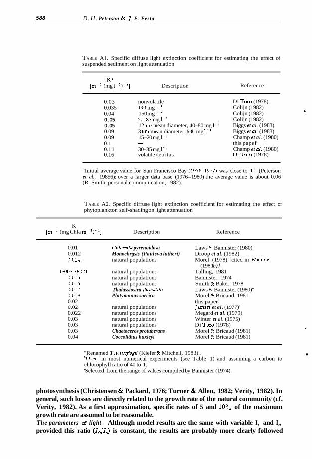
phytoplankton sinking velocities are not a commonly observed parameter in phytoplankton field ecology (Kalff & Knoechel, 1978). Nevertheless, a high value appears to be about 9 m d-' as illustrated by the large (150 pm diameter) diatom Coscinodiscus wailesii (Smyada, 1970; cited in Walsby & Reynolds, 1981). At the other end of the range certain forms of blue-green algae exhibit positive buoyancy (cf. Klemer et al. , 1982). In essence, estuarine phytoplankton sinking rates are poorly known but probably vary from slight positive buoyancy up to and perhaps exceeding 10 m d-'. Extinction coeficients Light attenuation by suspended sediment is largely determined by the concentration and to some extent the size of suspended sediment (Di Toro, 1978; Biggs et al., 1983). The few available estimates indicate a specific diffuse extinction

reasonable (Table Al). The specific extinction coefficient for phytoplankton chlorophyll (and accessory

pigments; cf. Morel & Bricaud, 1981) varies partly because of complex differences in pigment packaging (self-shading or sieve effect; cf. Latimer, 1982; Fukshansky, 198 1). Specific absorption varies with species, its size, the concentration of accessory pigments and other factors (cf. Morel & Bricand, 1981; Welschmeyer & Lorenzen, 1981; Kiefer & Mitchell, 1983). A value of 0.02 or close to 0.02 m-' (mg chla m-3)- ' is commonly used as an average value for natural populations (Table A2). Carbon to chlorophyll ratio Determination of the carbon to chlorophyll ratio in natural phytoplankton communities is a nasty analytical problem partly because living phytoplankton biomass is contaminated with a large and variable matrix of detritus (Banse, 1977; Redalje & Laws, 1981). A further difficulty is that this ratio is not a simple physiological parameter; for instance, shade adaptation may decrease the carbon to chlorophyll ratio with decreasing growth-light intensities (Senger & Fleischhacker, 1978; Perry et al., 1981; Kiefer & Mitchell, 1983; and others). The carbon to chlorophyll ratio is assumed to be 40 to 1, although in this study other values may have served equally well (Table A3). Phytoplankton growth and respiration Maximum growth rates (optimal light, temperature and nutrients) of phytoplankton tend to decrease with increasing unicellular algae size. Maximum rates normalized to cell size show diatoms generally grow faster, approximately 2.5 to 1 d- ', than most dinoflagellates, about 1 to less than 0.5 d-' and other algae fall between these values or below dinoflagellate values (Banse, 1982). Rates of 1 to 0.5 (Table 1) are well within this range. Intuitively, we expect that average

rates when averaged over a relatively long time. Therefore, moderate values seem more consistent with the experimental design of this study than 'high' values because the model parameters are considered characteristic of values averaged over one month and longer. This possible distinction is worth noting but is not as critical as other observational and model uncertainties.

By delinition, when the carbon to chlorophyll ratio and maximum specific growth rate are selected, maximum productivity on a chlorophyll basis is also determined. At a carbon to chlorophyll ratio of 40 to 1 and a specific growth rate of 1 d-', maximum productivity is 1.7 mg C (mg Chl)-l h-'. As per above, such values are assumed to represent rates averaged over relatively long time scales and are lower than the typical maximum rates as observed in die1 experiments (cf. Harding et al., 1981).

Phytoplankton loss rates are very poorly known. Examples of natural phytoplankton respiration losses range from less than 5 to greater than 30% of carbon assimilated by

.

(I coefficient in the range of about 0.05 to 0.1 m-' (mg suspended sediment l-')-' is

A values of maximum growth rates are closer to moderate observed rates rather than high

588 D. H. Peterson & 7. F . Festa

TABLE Al. Specific diffuse light extinction coefficient for estimating the effect of suspended sediment on light attenuation

K* [m-' (mg I-')-'] Description Reference

0.03 0.035 0.04 0.05 0.05 0.09 0.09 0.1 0.1 1 0.16

nonvolatile 190 mg I-' 150 mg 1-' 30-87 mg 1-' 12 pm mean diameter, 40-80 mg 1-' 3 pm mean diameter, 5-8 mg 1- ' 15-20 mg 1-'

30-35 mg 1-' volatile detritus

-

Di Tor0 (1978) Colijn (1982) Colijn (1982) Colijn (1982) Biggs et al. (1983) Biggs et al. (1983) Champ et al. (1980) this papef Champ et al. (1980) Di Tor0 (1978)

5

"Initial average value for San Francisco Bay (1976-1977) was close to 0.1 (Peterson et al., 19856); over a larger data base (1976-1980) the average value is about 0.06 (R. Smith, personal communication, 1982).

TABLE A2. Specific diffuse light extinction coefficient for estimating the effect of phytoplankton self-shading on light attenuation

K [m-' (mg Chla m-3)-'] Description Reference

0.01 Chlorella pyrenoidosa Laws & Bannister (1980) 0.012 Monochrgsis (Paulova lutheri) Droop et al. (1982) 0.014 natural populations Morel (1978) [cited in Malone

(198 1 b)] 0.008-0.021 natural populations Talling, 1981

0.016 natural populations Bannister, 1974 0.016 natural populations Smith & Baker, 1978 0,017 Thalassiosira jluviatilis Laws & Bannister (1980)" 0.018 Platymonas suecica Morel & Bricaud, 1981 0.02 - this paperb

0.02 natural populations Jamart et al. (1977)' 0.022 natural populations Megard et al. (1979) 0.03 natural populations Winter et al. (1975) 0.03 natural populations Di Tor0 (1978) 0.03 Chaetoceros protuberans Morel & Bricaud (1981) 0.04 Coccolithus huxleyi Morel & Bricaud (1981)

r(

"Renamed T. weissjlogii (Kiefer & Mitchell, 1983). , *Used in most numerical experiments (see Table 1) and assuming a carbon to chlorophyll ratio of 40 to 1. 'Selected from the range of values compiled by Bannister (1974).

.

photosynthesis (Christensen & Packard, 1976; Turner & Allen, 1982; Verity, 1982). In general, such losses are directly related to the growth rate of the natural community (cf. Verity, 1982). As a first approximation, specific rates of 5 and 10% of the maximum growth rate are assumed to be reasonable. The parameters of light Although model results are the same with variable I, and I,, provided this ratio (Z,/ZJ is constant, the results are probably more clearly followed


TABLE A3. Examples of the ratio of phytoplankton carbon to chlorophyll (by weight)

Reference C/Chl Description

15 12-36 18-41 20-60

40 40 40 49 50

25-80

natural populations natural populations Thalassiosira fluviatilis natural populations natural populations natural populations natural populations natural populations natural populations natural populations

Winter et al. (1975) Jamart et al. (1979) Laws & Bannister (1980) Jamart et al. (1977) this paper Cloern et al. (1983) Li et al. (1983) Cloern (1982) Di Tor0 et al. (1971) Parsons et al. (1977)

when referenced to absolute values of light intensity. This is established as follows. For purposes of steady-state simulations, a nearly maximum value of summer sunlight averaged over 24 h is estimated to be approximately 3.6 x 10l6 quanta cmT2 s- l (600 pE rn-’s-’) PAR and I, for phytoplankton is commonly about 10% full sunlight (Peterson et al., 1985a, b) . In this first study the selection of I , is somewhat arbitrary and a value of 0.3 x 10l6 quanta cm-2 s- l (50 pEm-’s-’> is assumed. This value is at the low range of a large number of values which fall in the relatively narrow range of 50 to 1 2 0 ~ E m - ~ sC1 (Talling, 1957a, by and cited in Harris, 1981, p. 136). Again, this is consistent with the parameters selected above in the sense that I , may or may not decrease, but typically does not increase with decreasing maximum productivity (cf. Platt et al., 1980; Peterson et al., 1985a, b). In this study I, is assumed to be a constant. For example, when Z,/Z, equals 6, then I , is 1.8 x 10l6 quanta cm-’s-l PAR.

Date post:	28-May-2018
Category:	Documents
Upload:	lecong
View:	217 times
Download:	0 times

Numerical Simulation of Phytoplankton Productivity in ... · Numerical Simulation of Phytoplankton...

Documents