Numerical solutions of BSDEs: A-posteriori estimates and ... · Numerical solutions of BSDEs:...

Numerical solutions of BSDEs:A-posteriori estimates and

enhanced least-squares Monte Carlo

Dissertation zur Erlangung des Grades der

Doktorin der Naturwissenschaften derNaturwissenschaftlich-Technischen Fakultaten der

Universitat des Saarlandes (Dr. rer. nat.)

eingereicht

am 31. Mai 2012

in Saarbrucken

von

Jessica Steiner

lalala

Tag des Kolloquiums: 11. September 2012

Mitglieder des Prufungsausschusses:

Vorsitzender: Prof. Dr. Anselm Lambert

Protokollfuhrer: Dr. Moritz Weber

1. Berichterstatter: Prof. Dr. Christian Bender

2. Berichterstatter: Prof. Dr. Bruno Bouchard

Dekan: Prof. Dr. Mark Groves

To my parents

lalala

Eidesstattliche Versicherung

Hiermit versichere ich an Eides statt, dass ich die vorliegende Arbeit selbststandigund ohne Benutzung anderer als der angegebenen Hilfsmittel angefertigt habe. Dieaus anderen Quellen oder indirekt ubernommenen Daten und Konzepte sind unterAngabe der Quelle gekennzeichnet. Die Arbeit wurde bisher weder im In- noch imAusland in gleicher oder ahnlicher Form in einem Verfahren zur Erlangung einesakademischen Grades vorgelegt.

Saarbrucken, 31. Mai 2012

(Dipl.-Math. Jessica Steiner) lalalala

Abstract

Backward stochastic differential equations (BSDEs) are a powerful tool in financialmathematics. Important examples are option pricing or portfolio selection problems.In non-linear cases BSDEs are usually not solvable in closed form and approximationbecomes then inevitable. Several proposals for solving BSDEs numerically have beenpublished in recent years, including an analysis of the related approximation error.

The first part of this theses is devoted to the problem that a direct a-posteriorievaluation of the L2-error between the true solution and some numerical solutionis usually impossible. Therefore, we present an a-posteriori criterion on the ap-proximation error, which is computable in terms of the numerical solution only andallows us to judge the numerical solution.

Secondly, we pick up the idea of Gobet, Lemor and Warin (Ann. Appl. Probab., 15,2172 – 2202 (2005)) to generate numerical solutions by least-squares Monte Carlo. Wesuggest to use function bases that form a system of martingales. A complete analysisof the approximation error shows, that in contrast to original least-squares MonteCarlo, the convergence behaviour can be significantly enhanced by the martingaleproperty of the bases.

v

Deutsche Zusammenfassung

Ruckwartsgerichtete stochastische Differentialgleichungen (BSDEs) sind ein viel-seitiges Instrument in der Finanzmathematik. Optionsbepreisung oder Portfolio-Auswahlprobleme sind wichtige Beispiele dafur. In nichtlinearen Fallen sind BSDEsin der Regel jedoch nicht geschlossen losbar, weshalb in den vergangenen Jahrenzahlreiche numerische Ansatze zusammen mit einer theoretischen Analyse ihresApproximationsfehlers vorgestellt worden sind.

Der erste Teil dieser Arbeit beschaftigt sich mit dem Problem, dass eine direkte a-posteriori Berechnung des L2-Fehlers zwischen der unbekannten echten und der nu-merischen Losung oftmals unmoglich ist. Deshalb prasentieren wir ein a-posterioriKriterium, das nur von der numerischen Losung abhangt und eine Beurteilungdieser erlaubt.

Der zweite Teil baut auf der Idee von Gobet, Lemor und Warin (Ann. Appl.Probab., 15, 2172 – 2202 (2005)) auf, numerische Losungen mit Hilfe eines Kleinste-Quadrate-Monte-Carlo-Verfahrens zu erzeugen. Wir schlagen Funktionenbasen vor,die ein System von Martingalen bilden. Eine vollstandige Analyse des Approxima-tionsfehlers zeigt, dass das Konvergenzverhalten durch die Martingaleigenschafterheblich verbessert wird im Vergleich zum ursprunglichen Verfahren.

vii

Contents

Abstract v

Deutsche Zusammenfassung vii

1 Introduction 11.1 Background on BSDEs and their numerical solution . . . . . . . . . . . 11.2 Problem description . . . . . . . . . . . . . . . . . . . . . . . . . . . . . 3

2 Preliminaries 92.1 Some important results on BSDEs . . . . . . . . . . . . . . . . . . . . . . 92.2 The least-squares Monte Carlo algorithm for BSDEs . . . . . . . . . . . 10

2.2.1 Discrete-time approximators . . . . . . . . . . . . . . . . . . . . 102.2.2 Least-squares Monte Carlo estimation of conditional expecta-

tions . . . . . . . . . . . . . . . . . . . . . . . . . . . . . . . . . . 122.2.3 Projection error within least-squares Monte Carlo estimation . . 132.2.4 Simulation error within least-squares Monte Carlo estimation . 182.2.5 Qualitative analysis of the error sources and their configuration 20

3 Error criteria for BSDEs 233.1 Global a-posteriori error criterion . . . . . . . . . . . . . . . . . . . . . . 23

3.1.1 Global a-posteriori estimates for discrete-time BSDEs . . . . . . 243.1.2 Examples for the application on numerical approaches . . . . . 293.1.3 Global a-posteriori criterion for continuous BSDEs . . . . . . . . 313.1.4 The a-posteriori error criterion for typical examples of BSDEs . 41

3.2 Local error criterion for approximate solutions obtained by projections 443.3 Non-linear control variates for BSDEs . . . . . . . . . . . . . . . . . . . 493.4 Numerical examples . . . . . . . . . . . . . . . . . . . . . . . . . . . . . 50

3.4.1 A non-linear decoupled FBSDE with known closed-form solution 503.4.2 A non-linear option pricing problem . . . . . . . . . . . . . . . . 58

4 Enhancing the least-squares MC approach by martingale basis functions 614.1 Construction of the simplified algorithm and examples for martingale

bases . . . . . . . . . . . . . . . . . . . . . . . . . . . . . . . . . . . . . . 614.2 Error sources and their contribution to the approximation error . . . . 66

4.2.1 Projection error . . . . . . . . . . . . . . . . . . . . . . . . . . . . 664.2.2 Truncation error . . . . . . . . . . . . . . . . . . . . . . . . . . . . 694.2.3 Simulation error . . . . . . . . . . . . . . . . . . . . . . . . . . . 75

4.3 The overall approximation error and its comparison with original LSMC 89

ix

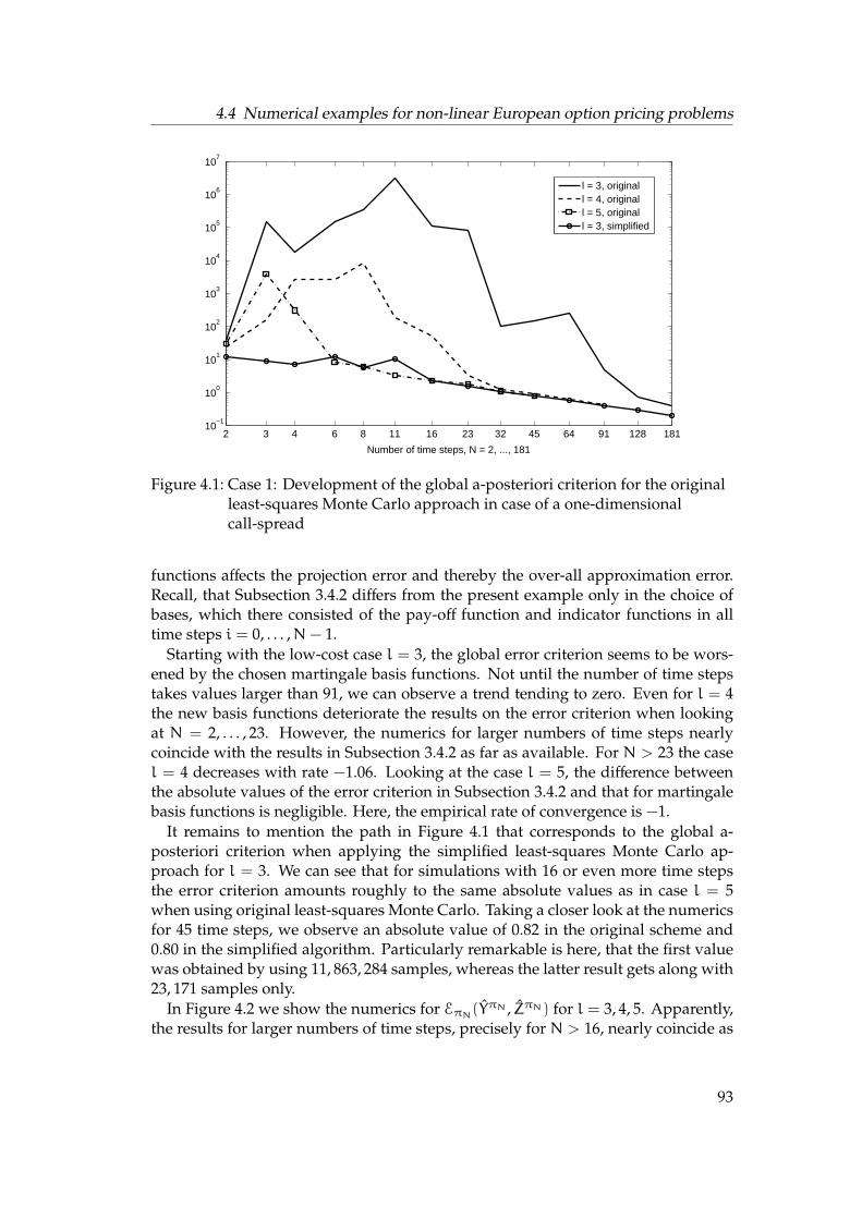
4.4 Numerical examples for non-linear European option pricing problems 914.4.1 Call-spread option . . . . . . . . . . . . . . . . . . . . . . . . . . 914.4.2 Pricing of a straddle - Simulation with estimated martingales . 96

A Some results on nonparametric regression and VC dimension 101

Acknowledgements 103

Bibliography 103

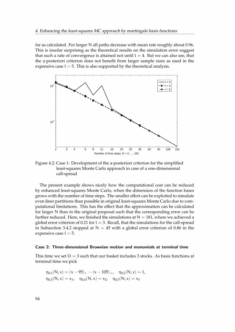
List of figures 109

List of tables 109

1 Introduction

1.1 Background on BSDEs and their numerical solution

The theory of backward stochastic differential equations (BSDEs) is a rather youngresearch field and its subjects first popped up in the context of stochastic control. Itwas Bismut (1973) who carried Pontryagin’s maximum principle over to stochasticcontrol problems and showed that the pair of adjoint processes solves a linear BSDE.

The actual foundation for BSDE theory was laid later on by Pardoux and Peng(1990), who examined non-linear BSDEs and proved the well-posedness of suchequations in case of a Lipschitz continuous driver. In the following, numerouspublications were devoted to an extension of this result.

One branch was engaged with the relaxation of the Lipschitz condition on thedriver. For instance, see Lepeltier and San Martın (1997), who examined BSDEs withcontinuous driver of linear growth, or Kobylanski (2000) on BSDEs with drivers ofquadratic growth. An overview is given in El Karoui and Mazliak (1997). Anotherimportant aspect was the analysis of the connection between solutions of BSDEsand viscosity solutions for quasilinear parabolic partial differential equations byPardoux and Peng (1992). Based on this, the notion of forward backward stochasticdifferential equations (FBSDEs) was developed and a generalization of the Feynman-Kac formula was obtained. A detailed introduction on this topic is also available inMa and Yong (1999). Particularly, FBSDEs became a useful tool in the field of financialmathematics. Amongst these are pricing and hedging of European options in caseswith constraints or utility optimization problems. An extension to American optionsby BSDEs with reflection was shown in El Karoui et al. (1997a). A comprehensivesurvey on the application of BSDEs in finance is given by El Karoui et al. (1997).

Whereas the research on BSDEs was indeed fruitful from its kick-off in the earlynineties on, the pioneering work on the numerics of BSDEs initially advanced muchslower. Bally (1997) was the first who proposed a time discretization scheme as anumerical approach towards the solution of BSDEs. Then it remained to solve aseries of linear BSDEs within each time step. The main drawback of this approachis that the time steps have to be chosen randomly in order to avoid any strongerregularity assumptions on the coefficients of the BSDE that go beyond the Lipschitzcontinuity of the driver.

Chevance (1997) presented a fully implementable numerical attempt to solve adecoupled FBSDE with a deterministic time discretization. However, this was con-nected with quite strong regularity conditions on the coefficient of both the forwardand the backward SDE. It was Zhang (2001) who offered a way out of this dilemma byformulating conditions such that the control part of the solution of a BSDE behavessomewhat ’nice’. These conditions include Lipschitz conditions on the coefficients

1

1 Introduction

of the forward SDE and the possibly path-dependent terminal condition of the BSDEand are merely an addition to the Lipschitz continuity of the driver. In particular,he introduced the notion of L2-regularity for stochastic processes and showed thatthese mild extra conditions are sufficient for the L2-regularity of the control part andthus also for the convergence of a deterministic time discretization with order 1/2 inthe number of time steps.

Slightly different, but somewhat more natural ways of time discretization fordecoupled FBSDEs were examined in Bouchard and Touzi (2004) and Lemor et al.(2006), however they both benefit from the L2-regularity results obtained by Zhang(2001). In contrast to the algorithm suggested in Lemor et al. (2006), the approachby Bouchard and Touzi (2004) is characterized by its implicit formulation. Thereare several proposals to turn this idea into a tractable algorithm by using some sortof Picard iteration. This can be done within each time step, see Gobet et al. (2005),or globally by an iteration that restarts at terminal time after having completedthe iteration step along the entire partition, see Bender and Denk (2007). Bothmethods have to deal with the problem of nested conditional expectations, on theone hand along the partition of the time interval and on the other one along thePicard iterations. Bender and Denk (2007) showed that the global Picard iterationis more favorable concerning the error propagation that arises when estimatingconditional expectations. The work of Gobet and Labart (2010) is also in the spiritof global Picard iteration connected with a control variate technique. Another wayof variance reduction within a global Picard scheme was presented in Bender andMoseler (2010), who applied the so-called importance sampling technique that makesuse of measure change to receive more samples in ’interesting’ regions.

Extensions to this research can be found in Gobet and Makhlouf (2010) and Geisset al. (2011), who supposed the terminal condition to be irregular. Even then the errordue to time discretization tends to zero, although the convergence rate is in this caseslower for equidistant partitions of the time interval. However, a clever choice ofpartition can improve this rate significantly, in certain cases up to 1/2 in the numberof time steps. Worth mentioning is the work of Imkeller et al. (2010) and also Richou(2011) on numerical approximation of BSDEs with drivers of quadratic growth in thecontrol part. In the first case, the non-Lipschitz continuity was tackled by imposinga truncation on the driver and approximating the true BSDE by a series of truncatedones. In the latter one time-dependent bounds for the control part within the timediscretization scheme were incorporated.

Regarding coupled FBSDEs, Bender and Zhang (2008) proposed a combination oftime discretization and Markovian iteration to tackle the coupling. They formulatedalso sufficient conditions for a time discretization error that decreases with rate 1/2 inthe number of time steps. The case of FBSDEs with jumps was covered by Bouchardand Elie (2008).

Whatever type of time discretization is chosen, at the end of the day one is con-fronted with the problem of estimating conditional expectations. This stems fromthe backward property of BSDEs and the necessity to adapt the approximation to theavailable information at each time step. In recent years several proposals have beenestablished to cope with this problem. Bouchard and Touzi (2004) applied Malliavin

2

1.2 Problem description

Monte Carlo for the estimation of conditional expectations. By means of Malliavinintegration by parts, these can be expressed by a ratio of expectations, that can beestimated via Monte Carlo simulation. See also Bouchard et al. (2004).

An alternative was considered in Bally and Pages (2003), who chose the quantiza-tion tree method for the estimation of conditional expectations. Roughly speaking,the idea is to project the time-discretized underlying diffusion process on discretestate spaces and to estimate the transition probabilities between the single time stepsby simulation. The conditional expectations are then easily computable weightedsums. Delarue and Menozzi (2006) transferred this idea to the numerical solution ofcoupled FBSDEs.

Only recently, Crisan and Manolarakis (2010) exploited the cubature method forthe estimation of conditional expectations for the generation of numerical solutionsof BSDEs.

Last but not least, Gobet et al. (2005) tackled the estimation of conditional expecta-tions by least-squares Monte Carlo. This approach can be understood as a two-stepprocedure that starts with a projection on a function basis and next solves the re-sulting minimization problem by Monte Carlo simulation. We will explain this idealater on in more detail.


Let (Ω,F,P) be a probability space, whereF = (Ft, t > 0) is the augmented filtrationgenerated by a D-dimensional Brownian motion W = (W1, . . . ,WD)∗. Here the stardenotes matrix transposition. We fix further a terminal time T > 0. Then our firstbranch of studies starts with a backward stochastic differential equation (BSDE) ofthe form

Yt = ξ−

∫Tt

f(u, Yu,Zu)du−

∫Tt

ZudWu, (1.1)

where the data is assumed to satisfy

Assumption 1. (i) The terminal condition ξ is a real valued, square-integrable, FT -measurable random variable.

(ii) The driver is a measurable function f : Ω × [0, T ] × R × RD → R, such that(f(t, 0, 0), 0 6 t 6 T) is a continuous, F-adapted process with

∫T0 E|f(t, 0, 0)|2dt < ∞.

Moreover, f is Lipschitz in its spatial variables with constant κ uniformly in (t,ω). Note,that the stochastic variable is suppressed in the above equation.

The solution of (1.1) consists of a pair of adapted stochastic processes (Y,Z), whereYt is real valued and Zt = (Z1,t, . . . ,ZD,t) is RD-valued. However, in most caseswe cannot state a closed-form solution for (1.1) and a workaround by numericalapproaches becomes highly interesting in order to obtain at least an approximationof (Y,Z).

Let us assume, we conducted some arbitrary numerical scheme, that is based ona discretization π = t0, . . . , tN of the interval [0, T ], namely 0 = t0 < t1 < . . . <

3

1 Introduction

tN = T , and its result is the pair (Yπti , Zπti)ti∈π. Then, a quite natural wish is to get

information about the approximation error. Precisely, we want to check

sup06t6T

E|Yt − Yπti|2 +

∫T0E|Zt − Z

πti|2dt

and judge thereby, if the chosen numerical approach was successful. Here, the pair(Yπt , Zπt )06t6T denotes the RCLL-extension of (Yπti , Z

πti)ti∈π by constant interpola-

tion. But, as the true solution is usually unknown to us, it is not possible to computethe approximation error directly or even estimate it, e. g. by Monte Carlo simulation.

Nevertheless, we want to shed some light on the question, whether the pair(Yπti , Z

πti)ti∈π is a good approximation. For this purpose we introduce a so-called

’global’ a-posteriori error criterion. Suppose that (Yπti , Zπti)ti∈π is adapted to a filtra-

tion G = (Gt, 0 6 t 6 T) such that Ft ⊆ Gt for t ∈ [0, T ]. That means, G is enlargedin comparison to F and W is still a Brownian motion with respect to G. But Gtican also contain additional information, for instance induced by copies of Wti thatwere required for the approximation of (Yπti , Z

πti)ti∈π. Least-squares Monte Carlo

simulation for BSDEs is an example for the incorporation of such copies. Then theglobal a-posteriori criterion checks by

Eπ(Yπ, Zπ) := E[|ξπ − YπtN |

2| Gt0 ] + max16j6N

E[|Yπtj − Yπt0

−

j−1∑i=0

fπ(ti, Yπti , Zπti)(ti+1 − ti) −

j−1∑i=0

Zπti(Wti+1 −Wti)|2| Gt0 ], (1.2)

if the approximate solution is ’close to solving’ (1.1). Here, (ξπ, fπ) denotes anapproximation of (ξ, f) living on the time grid π. Contrary to the approximationerror, it is possible to simulate (1.2), as it involves only approximate, hence knownsolutions and approximate data. In a first step, we will develop upper and lowerestimates on the approximation error in terms of this criterion. These estimatesrequire only standard Lipschitz conditions on the driver f.

After that, we apply the global error criterion on a forward backward stochasticdifferential equation (FBSDE) denoted by

St = s0 +

∫t0b(u,Su)du+

∫t0σ(u,Su)dWu

Yt = φ(S) −

∫Tt

F(u,Su, Yu,Zu)du−

∫Tt

ZudWu.(1.3)

This system is supposed to fulfill

Assumption 2. We call s0 ∈ RD the initial condition of S. The functions b : [0, T ]×RD →RD , σ : [0, T ]×RD → RD×D and F : [0, T ]×RD ×R×RD → R are deterministic andthere is a constant κ such that

|b(t, s) − b(t ′, s ′)|+ |σ(t, s) − σ(t ′, s ′)|+ |F(t, s,y, z) − F(t ′, s ′,y ′, z ′)|

6 κ(√t− t ′ + |s− s ′|+ |y− y ′|+ |z− z ′|)

4


for all (t, s,y, z), (t ′, s ′,y ′, z ′) ∈ [0, T ]×RD×R×RD. The terminal condition ξ = φ(S)

is a functional on the space of RD-valued RCLL functions on [0, T ], that satisfies the L∞-Lipschitz condition

|φ(s) − φ(s ′)| 6 κ sup06t6T

|s(t) − s ′(t)|

for all RCLL functions s, s ′. In addition to that

sup06t6T

(|b(t, 0)|+ |σ(t, 0)|+ |F(t, 0, 0, 0)|) + |φ(0)| 6 κ,

where 0 denotes the constant function taking value 0 on [0, T ].

Clearly, we look at a BSDE with data ξ = φ(S) and f(t,y, z) = F(t,S,y, z), whereF is stochastic through S only. The above system is called decoupled as the forwardSDE is independent of the pair (Y,Z). Given Assumption 2 it is easy to check, thatthe conditions of Assumptions 1 are satisfied as well.

Concerning this type of FBSDEs, we will take a closer look on a numerical methodthat combines a backwards time discretization scheme with the least-squares MonteCarlo approach for the estimation of conditional expectations to generate approxi-mations of the processes Y and Z. This method was already employed by Gobet etal. (2005) and Lemor et al. (2006) in this setting and aims at replacing the conditionalexpectations by a projection on a subspace of L2(Fti) for each time step ti.

We will review the approximation error of this scheme and explain its error sources,in particular the time discretization error, the projection error and the simulationerror. Moreover, we will recall how the parameters of the latter one can be fixedsuch that the overall approximation error converges with the same rate as the timediscretization error.

Additionally, we present for this setting a ’local’ a-posteriori error criterion, that isdenoted by

Elocπ,j (Yπ, Zπ) :=

N−1∑i=j

E|Yπti+1− Yπti − F(ti, S

πti

, Yπti , Zπti)(ti+1 − ti)

− Zπti(Wti+1 −Wti)|2,

for j = 0, . . . ,N − 1. It is meant to give further information about the projectionerror, which is expressed in terms of the L2-error between a time-discretized solution(Yπti , Z

πti)ti∈π and its best projection on the selected function basis. Precisely, it turns

out that a small local error criterion is a necessary condition for a small projectionerror. Furthermore, it allows us to detect those time steps for which the projectionfunctions were picked inappropriately.

The second branch of our studies is devoted to a modification of the least-squaresMonte Carlo approach. Induced by the time discretization we are confronted with

5

1 Introduction

the estimation of

E[Yπti+1− F(ti, Sπti , Y

πti

, Zπti)(ti+1 − ti)| Fti ]

1(ti+1 − ti)

E[(Wti+1 −Wti)Yπti+1

| Fti ],

by a linear combination of basis functions. The estimation of the first conditionalexpectation leads to the definition of Yπti , whereas the estimation of the latter one isrequired for Zπti . Motivated by a kind of variance reduction for FBSDEs, we assumethat the function bases form a system of martingales. Let (Xπti)ti∈π be a F-adaptedMarkov process and η(i+ 1,Xπti+1

) a basis function at time ti+1 such that

(i) its conditional expectation related to Fti is computable in closed-form,

(ii) the conditional expectation of this function multiplicated with the dth compo-nent of the Brownian incrementWti+1 −Wti can be evaluated related to Fti forall d = 1, . . . ,D.

This suggestion is inspired by Glasserman and Yu (2004) in the field of pricingAmerican options. Assumption (i) is related to the approximation of Y and ensuresthat (η(i,Xπti)ti∈π forms a martingale with respect to F, that is available in closedform. In this setting, the estimation of conditional expectations becomes obsoletefor all linear terms, as they can be computed in closed form under the assumptionof martingale basis functions. E. g., let Yπ at time ti+1 be a linear combination ofso-called martingale basis functions, then we can figure out its conditional expecta-tion by the martingale property. This simplifies the approximation of Yπti , as onlyE[F(ti, Sπti , Y

πti

, Zπti)| Fti ] remains to be estimated.Moreover, by (ii) the evaluation ofE[(Wd,ti+1−Wd,ti)Y

πti+1

| Fti ],d = 1, . . . ,D, whichstems from the time discretization of Zd, becomes possible in closed form. Thatmeans, we do not require any additional estimation of conditional expectations forthe approximate solution of Zd. This is particularly interesting in high-dimensionalproblems, when D > 1. Clearly, in the martingale basis approach the amount ofconditional expectations to be estimated is the same, no matter if the BrownianmotionW is one-dimensional or multi-dimensional.

We give several examples for ’martingale type’ basis functions and conduct after-wards a detailed analysis of the approximation error and its error sources. It turnsout that the projection error and the simulation error can be reduced significantly incontrast to the original least-squares Monte Carlo approach.

The rest of this thesis is organized as follows. In Chapter 2 we review some impor-tant results on BSDEs that are essential for this paper. Additionally, we explain theleast-squares Monte Carlo approach and its approximation error in detail. Chapter3 is devoted to the a-posteriori error criteria. Apart from the global criterion, wepresent the local one for approximate solutions that where obtained by replacingconditional expectations by projections. This chapter ends with the introduction ofnon-linear control variates for (F)BSDEs inspired by variance reduction methods.Therefore, we will diminish the original BSDE by some BSDE, that is solvable in

6


closed-form and is likely to ’explain’ the main part of the original one. Approx-imation has then to be applied to the remainder BSDE. The chapter also includesnumerical examples. In Chapter 4 we introduce the enhanced least-squares MonteCarlo scheme and examine the approximation error in its very detail. Again, thechapter is finished by numerical examples.

7

2 Preliminaries

2.1 Some important results on BSDEs

Before turning to the numerical solution of BSDEs and their validation, it is essentialto know if the problem in (1.1) is well-defined. To this end, we cite a result of Pardouxand Peng (1990).

Theorem 1. We suppose that the data (ξ, f) satisfy Assumption 1. Then there is a uniquepair of predictable processes (Y,Z) with

E

∫T0|Yt|

2dt <∞, E

∫T0|Zt|

2dt <∞,

that solves the differential equation (1.1).

During our thesis we require some standard regularity estimates on the processesS and Y several times. These results can also be found in Zhang (2004), who moregenerally considers the Lp-norm for p > 2 instead of the case p = 2 only.

Lemma 2. Let Assumption 1 be fulfilled and (Y,Z) be an adapted solution of (1.1). Thenthere is a constant C depending on T , κ and the data (ξ, f) only such that

E|Yt − Ys|2 6 C|t− s|+ C

∫ts

E|Zu|2du.

Lemma 3. Let Assumption 2 be fulfilled and S be a solution of the forward SDE in (1.3).Then there is a constant C depending on T , κ, s0 and the data (b,σ) such that

E|St − Ss|2 6 C|t− s|.

It was Zhang (2001), who made an important contribution concerning the regu-larity of the process Z. Beyond inventing the notion of L2-regularity by

N−1∑i=0

∫ti+1

ti

E∣∣∣Zt −

1∆iE[ ∫ti+1

ti

Zsds∣∣∣Fti

]∣∣∣2dt,

he showed that rather mild conditions are sufficient to obtain a regularity rate oforder 1/2 in the number of time steps of a deterministic partition of the time interval[0, T ]. This result is essential for the convergence of a discrete-time approximation of(Y,Z), as will be reviewed in the next subsection.

9

2 Preliminaries

Theorem 4. We suppose that Assumption 2 is satisfied. Let π = t0, . . . , tN be a partitionof [0, T ] with 0 = t0 < . . . < ti < . . . < tN = T . Then there is a constant C > 0 dependingon T , κ and s0 only such that

N−1∑i=0

∫ti+1

ti

E∣∣∣Zt −

1∆iE[ ∫ti+1

ti

Zsds∣∣∣Fti

]∣∣∣2dt 6 C max

06i6N−1|ti+1 − ti|,

where C is independent of π.

2.2 The least-squares Monte Carlo algorithm for BSDEs

The least-squares Monte Carlo algorithm for BSDEs was initially proposed by Gobetet al. (2005) for the numerical solution of FBSDEs as formulated in (1.3) and is basedon a discrete-time approximation of (Y,Z). Then least-squares Monte Carlo comesinto play in order to tackle the estimation of conditional expectations, that ariseduring the time discretization. We explain both steps in detail in the followingsubsections.

2.2.1 Discrete-time approximators

There are several proposals for the time discretization of (Y,Z), for instance seeBouchard and Touzi (2004) or Zhang (2004). Here, we will explain step by stepthe scheme that was proposed by Lemor et al. (2006). Considering the time gridπ = t0, . . . , tN of [0, T ] with 0 = t0 < . . . < ti < . . . < tN = T , we define |π| =max06i6N−1 |ti+1 − ti| and suppose that a discrete-time approximation Sπti , ti ∈ πof the forward SDE S is at hand that fullfills

Assumption 3. The process (Sπti)ti∈π is an adapted Markov process. Moreover, there is aconstant C > 0 such that

max06i6N

E|Sti − Sπti|2 6 C|π|.

In numerous financial settings the forward SDE consists of a geometric Brownianmotion, that can be sampled perfectly on the time grid π. For many other cases theEuler scheme, e. g., provides a suitable approximation satisfying Assumption 3.

For the time discretization of (Y,Z) we define ∆i := ti+1 − ti, ∆Wd,i = Wd,ti+1 −Wd,ti and ∆Wi = (∆W1,i, . . . ,∆WD,i)

∗. Due to the definition of the BSDE we have

Yti = Yti+1 −

∫ti+1

ti

F(u,Su, Yu,Zu)du−

∫ti+1

ti

ZudWu.

Inspired by this equality, we replace the integrals by their discrete counterparts andreceive the relation

Yti ≈ Yti+1 − ∆iF(ti,Sti , Yti ,Zti) − Zti∆Wi. (2.1)

10


Next, we multiply (2.1) with the Brownian increment ∆Wd,i and take after that theconditional expectation. Thus, we can derive from

0 ≈ E[Yti+1∆Wd,i| Fti ] − Zd,ti∆i

an approximation Zπti , provided that Yπti+1is given:

Zπti =1∆iE[(∆Wi)

∗Yπti+1| Fti ].

For the time discretization of the Y-part, we take the conditional expectation in (2.1)and obtain

Yti ≈ E[Yti+1 − ∆iF(ti,Sti , Yti ,Zti)| Fti ]≈ E[Yti+1 − ∆iF(ti,Sti , Yti+1 ,Zti)| Fti ].

In the last step we switched from Yti to Yti+1 , which turns the relation into an explicitone. Hence, we define for Sπti , Y

πti+1

and Zπti known,

Yπti = E[Yπti+1

− ∆iF(ti, Sπti , Yπti+1

, Zπti)| Fti ].

Now, we want to combine these considerations to a full description of the timediscretization scheme, that starts backwards in time with an approximation ξπ of theterminal condition. We achieve a time-discretized approximation (Yπ,Zπ) of (Y,Z)by conducting for all i = N− 1, . . . , 0

YπtN = ξπ,


∗Yπti+1| Fti ],

Yπti = E[Yπti+1


, Zπti)| Fti ].

(2.2)

Using constant interpolation we get processes (Yπt ,Zπt ), t ∈ [0, T ]. Zhang (2004) andBouchard and Touzi (2004) introduced quite similar schemes. Roughly speaking,they differ from (2.2) due to the variables that are plugged in the driver. Particularly,the latter authors evaluate the driver F at (ti, Sπti , Y

πti

, Zπti), which leads to an implicitdefinition of Yπti . All approaches have in common that under Assumptions 2 and3 the time discretization error in the L2-sense is of order 1/2 in the number of timesteps plus an error concerning the approximate terminal condition, i. e.

sup06t6T

E|Yt − Yπt |

2 +

∫T0E|Zt − Z

πt |

2dt 6 C|π|+ CE|ξ− ξπ|2,

see Lemor et al. (2006) for a proof with respect to the above setting.Although (2.2) is formulated explicitly in time, it incorporates the computation of

(nested) conditional expectations, that in many cases cannot be figured out in closedform. Thus, estimation of conditional expectations is an important problem, when

11

2 Preliminaries

it comes to solving BSDEs numerically. In the next subsection we will review theleast-squares Monte Carlo method as an estimation tool for this purpose.

Before going into the details, we endow the time-discretized solution with a kindof Markovian structure. To this end, we establish a multivariate Markov process(Xπti)ti∈π such that its first component matches the discretized SDE (Sπti)ti∈π. In sucha framework we can formulate the approximate terminal condition byξπ = φπ(XπtN),even if the true terminal condition is path dependent, e.g. φ(S) = max06t6T St orφ(S) = 1/T

∫T0 Stdt. Several examples for an appropriate construction of (Xπti)ti∈π

can be found in Gobet et al. (2005). In view of the Markovianity of (Xπti ,Fti)ti∈π wecan then rephrase algorithm (2.2). For i = N− 1, . . . , 0 we have

YπtN = φπ(XπtN),


∗Yπti+1|Xπti ],

Yπti = E[Yπti+1


, Zπti)|Xπti].

(2.3)

Hence, there are functions yπi (x) and zπi (x) such that

Yπti = yπi (Xπti), Zπti = zπi (X

πti), i = 0, . . . ,N.

That means, the estimation of conditional expectation aims at finding deterministicfunctions as approximations for yπi and zπi . In the following we describe how thiscan be done by least-squares Monte Carlo.

2.2.2 Least-squares Monte Carlo estimation of conditional expectations

The least-squares Monte Carlo approach to the estimation of conditional expectationswas suggested in the context of pricing American options, see Longstaff and Schwartz(2001). Let U and X be some random variables. Then the computation of E[U| X] isequivalent to finding a function v(x) such that

v(X) = arg minvE|v(X) −U|2, (2.4)

where v is taken from the set of measurable functions with the propertyE|v(X)|2 <∞.We simplify the infinite-dimensional minimization problem to a finite-dimensionalone by defining a function basis η(x) with

η(x) = η1(x), . . . ,ηK(x) , K ∈N.

Thus, substituting (2.4) by the K-dimensional minimization problem

α = arg minα∈RK

E|η(X)α−U|2 (2.5)

reduces the original problem of finding a minimizing function to the problem offinding minimizing coefficients α. This yields an orthogonal projection of U on thesubspace of L2(σ(X)) spanned by η(X). Still, we have a problem that is in general

12


not solvable in closed form. Therefore, we replace the expectation operator in (2.5)by the sample mean and compute

αL = arg minα∈RK

1L

L∑λ=1

|η( Xλ )α− Uλ |2, (2.6)

where ( Xλ , Uλ ), λ = 1, . . . ,L are independent copies of (X,U). After setting

AL :=1√L

(η1( Xλ ) · · · ηK( Xλ )

)λ=1,...,L ,

we get a solution for (2.6) by

αL =1√L

((AL)∗AL

)−1(AL)∗

U1...UL

. (2.7)

In case (AL)∗AL is not invertible, we employ the pseudo inverse AL,+ of AL andcompute instead of (2.7) the following coefficients,

αL =1√LAL,+

U1...UL

.

In sum, we receive by η(X)αL the least-squares Monte Carlo estimator for E[U| X].The related approximation error is determined by two components, namely theprojection error, that reflects the adequacy of the chosen basis functions, and thesimulation error caused by the step from (2.5) to (2.6).

2.2.3 Projection error within least-squares Monte Carlo estimation

This subsection is devoted to the analysis of the projection error that occurs whenapplying the first step, see (2.5), of least-squares Monte Carlo estimation on (2.3).Since we are located in the setting of Lemor et al. (2006), the below stated result isof course part of their error analysis. However, Lemor et al. (2006) examine onlythe overall approximation error between a truncated version of the time-discretizedsolution and the simulated solution and the impact of the projection error is onlymentioned in passing. In order to distinguish different error sources, we provideLemma 5. To this end, we define for all i = 0, . . . ,N− 1 function bases

η0(i, x) := η0,1(i, x), . . . ,η0,K0,i(i, x)

for the estimation of yπi (x) and

ηd(i, x) := ηd,1(i, x), . . . ,ηd,Kd,i(i, x), d = 1, . . . ,D

13

2 Preliminaries

for the estimation of the dth component of zπi (x). Here, Kd,i stands for the dimensionof the function basis for d = 0, . . . ,D at time ti. In particular, we can select in eachtime step and for each of theD+1 estimation tasks a different basis. However, manynumerical examples for least-squares Monte Carlo are based on an identical basisfor the estimation of all conditional expectations within the same time step. Later onwe will show, how the estimation can benefit from different bases.

For the sake of clarity we denote by Pd,i,d = 0, . . . ,D, i = 0, . . .N− 1 the operatorsuch that for some FT -measurable random variable U

Pd,i(U) := ηd(i, Xπti)αd,i

with

αd,i = arg minα∈RKd,i

E|ηd(i, Xπti)α−U|2.

In other words Pd,i carries out an orthogonal projection on the subspace spannedby ηd(i, x), d = 0, . . . ,D. Replacing the conditional expectations in (2.3) by theprojection operator yields then the following algorithm:

Yπ,K0,NtN

= φπ(XπtN),

Zπ,Kd,id,ti

=1∆i

Pd,i(∆Wd,iY

π,K0,i+1ti+1

), d = 1, . . . ,D,

Yπ,K0,iti

= P0,i(Yπ,K0,i+1ti+1

− ∆iF(ti, Sπti , Yπ,K0,i+1ti+1

, Zπ,Kiti

)),

(2.8)

where Zπ,Kiti

= (Zπ,Kd,id,ti

)d=1,...,D. Again, for all i = 0, . . . ,N− 1 there are deterministic

functions yπ,K0,ii (x) and zπ,Kd,i

d,i (x) such that

Yπ,K0,i+1ti+1

= yπ,K0,ii (Xπti), Z

π,Kd,id,ti

= zπ,Kd,id,i (Xπti), d = 1, . . . ,D. (2.9)

In view of the definition of Pd,i,d = 0, . . . ,D, these functions can be written as linearcombinations of ηd(i, x), respectively.

Lemma 5. Let F be Lipschitz continuous in its spatial variables (y, z) with constant κ. Then

maxj6i6N

E|Yπti − Yπ,K0,iti

|2 +

N−1∑i=j

∆iE|Zπti− Zπ,Ki

ti|2

< C

N−1∑i=j

E|P0,i(Yπti) − Yπti |

2 + C

N−1∑i=j

D∑d=1

∆iE|Pd,i(Zπd,ti) − Z

πd,ti |

2,

for j = 0, . . . ,N− 1 with C > 0 being a constant depending on κ, T and D.

Gobet et al. (2005) provide an analysis of the projection error in a setting thatcombines least-squares Monte Carlo with Picard iterations in each time step.

14


Proof. We set ∆Fi = F(ti, Sπti , Yπ,K0,i+1ti+1

, Zπ,Kiti

) − F(ti, Sπti , Yπti+1

, Zπti) and exploit theLipschitz condition on F and Young’s inequality for some Γ to be defined later on.Hence,

E|∆Fi|2 6 κ2(1 + ΓD)E

[|Yπti+1

− Yπ,K0,i+1ti+1

|2 +1ΓD

|Zπti − Zπ,Kiti

|2]. (2.10)

Then we define

Yπti

= E[Yπ,K0,i+1ti+1

− ∆iF(ti, Sπti , Yπ,K0,i+1ti+1

, Zπ,Kiti

)|Xπti ].

and apply again Young’s inequality. Due to (2.10), we obtain for Γ = 1

E|Yπti − Yπti|2 6 (1 + (1 +D)κ2∆i)E|E[Y

πti+1

− Yπ,K0,i+1ti+1

|Xπti ]|2

+(∆i +

1(1 +D)κ2

)∆iκ

2(1 +D)E|Yπti+1− Y

π,K0,i+1ti+1

|2

+(∆i +

1(1 +D)κ2

)∆iκ

2 1 +D

DE|Zπti − Z

π,Kiti

|2.

(2.11)

Using the orthogonality of the projection Pd,i we receive

E|Zπd,ti − Zπ,Kd,id,ti

|2 = E|Zπd,ti − Pd,i(Zπd,ti

)|2 + E|Pd,i

(Zπd,ti

)− Z

π,Kd,id,ti

|2

= (I) + (II).(2.12)

As for (II), the definition of Zπd,ti and Zπ,Kd,id,ti

in (2.3) and (2.8) yields

(II) = E|Pd,i(∆−1i E[∆Wd,i(Y

πti+1

− Yπ,K0,i+1ti+1

)|Xπti ])|2

6 E|∆−1i E[∆Wd,i

Yπti+1

− Yπ,K0,i+1ti+1

− E[Yπti+1− Y

π,K0,i+1ti+1

|Xπti ]|Xπti ]|

2

6 ∆−1i E|Y

πti+1

− Yπ,K0,i+1ti+1

− E[Yπti+1− Y

π,K0,i+1ti+1

|Xπti ]|2

6 ∆−1i

(E|Yπti+1

− Yπ,K0,i+1ti+1

|2 − E|E[Yπti+1− Y

π,K0,i+1ti+1

|Xπti ]|2),

(2.13)

where the second step followed by the contraction property of the projection Pd,iand the third step by Holder’s inequality. Now we define a sequence (qi)i∈N withq0 = 1 and qi+1 = qi(1 + (1 + D)κ2∆i)(1 + ∆i). Turning back to (2.11), we firstexploit the estimates on the Z-part and multiply then with qi. Thus, for i < N− 1,

qiE|Yπti− Y

πti|2 6 qi(1 + (1 +D)κ2∆i)(1 + ∆i)E|Y

πti+1

− Yπ,K0,i+1ti+1

|2

+ qi(1 + (1 +D)κ2∆i)∆iD

D∑d=1

E|Pd,i(Zπd,ti) − Z

π,Kd,id,ti

|2

6 qi+1E|Yπti+1

− Yπti+1

|2 + qi+1E|P0,i+1(Yπti+1

) − Yπti+1|2

+ qi+1∆iD

D∑d=1


π,Kd,id,ti

|2,

15

2 Preliminaries

where we incorporated the relation

P0,i(Yπti − Y

πti

)= Y

π,K0,iti

− P0,i(Yπti) (2.14)

as well as the orthogonality and the contraction property of the projection P0,i. Incase i = N− 1 we have

qN−1E|YπtN−1

− YπtN−1

|2 6 qN∆N−1

D

D∑d=1

E|Pd,N−1(Zπd,tN−1

) − Zπ,Kd,N−1d,tN−1

|2,

since YπtN = Yπ,K0,NtN

. Taking the sum from i to N− 1 leads to

qiE|Yπti− Y

πti|2

6N−1∑j=i+1

qjE|P0,j(Yπtj) − Yπtj |

2 +

N−1∑j=i

qj+1∆j

D

D∑d=1

E|Pd,j(Zπd,tj) − Z

π,Kd,jd,tj

|2.

As ∆i < |π| < CT/N for some C > 0, we can conclude

qN <

(1 +

(1 +D)κ2CT

N

)N(1 +

CT

N

)N−−−−→N→∞ eCT(1+(1+D)κ2).

Hence,

maxj6i6N−1

E|Yπti − Yπti|2 6 eCT(1+(1+D)κ2)

N−1∑i=j+1


2

+ eCT(1+(1+D)κ2)N−1∑i=j

∆i

D∑d=1


π,Kd,id,ti

|2. (2.15)

In view of (2.14) and by exploiting the orthogonality of the projections, we receiveimmediately

maxj6i6N−1


|2

6 2 maxj6i6N−1

E|Yπti − P0,i(Yπti)|2 + 2 max

j6i6N−1E|P0,i(Y

πti− Y

πti)|2

6 C(N−1∑i=j


2 +

N−1∑i=j

D∑d=1


π,Kd,id,ti

|2)

.

Coming back to the estimates in (2.12) and (2.13), we apply the definition of Yπti and

16


the orthogonality of the projections. Clearly, we have for i = 0, . . . ,N− 2

∆iE|Zπd,ti − Z

π,Kd,id,ti

|2

6 E|Yπti+1− Y

πti+1

|2 + E|P0,i+1(Yπti+1

) − Yπti+1|2 − E|Yπti − Y

πti+ ∆i∆Fi|

2

+ E|Pd,i(Zπd,ti) − Z

π,Kd,id,ti

|2

6 E|Yπti+1− Y

πti+1

|2 − E|Yπti − Yπti|2 + 2∆iE|(Yπti − Y

πti)∆Fi|

2

+ E|P0,i+1(Yπti+1

) − Yπti+1|2 + ∆iE|Pd,i(Z

πd,ti) − Z

π,Kd,id,ti

|2

6 E|Yπti+1− Y

πti+1

|2 − E|Yπti − Yπti|2 + γ∆iE|Y

πti− Y

πti|2 +

∆iγE|∆Fi|

2

+ E|P0,i+1(Yπti+1

) − Yπti+1|2 + ∆iE|Pd,i(Z

πd,ti) − Z

π,Kd,id,ti

|2,

for some γ > 0. Now we apply (2.10) with Γ = 2 and consider also relation (2.14).Thus,

∆iE|Zπd,ti − Z

π,Kd,id,ti

|2 6 E|Yπti+1− Y

πti+1

|2 − E|Yπti − Yπti|2 + γ∆iE|Y

πti− Y

πti|2

+κ2(1 + 2D)∆i

γE[|P0,i+1(Y

πti+1

− Yπti+1

)|2 +1

2D|Zπti − Z

π,Kiti

|2]

+(

1 +κ2(1 + 2D)∆i

2Dγ

)E|P0,i+1(Y

πti+1

) − Yπti+1|2

+ ∆iE|Pd,i(Zπd,ti) − Z

π,Kd,id,ti

|2.(2.16)

Concerning E|P0,i+1(Yπti+1

− Yπti+1

)|2, we will make use of the contraction property ofthe projections. Then, we set γ = κ2(1 + 2D) and define a second sequence (qi)i∈Nwith q0 = 1 and qi+1 = qi(1 + ∆i). Multiplying (2.16) with qi and summing upfrom d = 1, . . . ,D and i = 0, . . . ,N− 1 yields

N−1∑i=j

qi∆iE|Zπti− Zπ,Ki

ti|2

6 Dκ2(1 + 2D)eCT maxj6i6N

qiE|Yπti− Y

πti|2 +

12

N−1∑i=0

qi∆iE|Zπti− Zπ,Ki

ti|2

+ C

N−1∑i=j

(E|P0,i(Y

πti) − Yπti |

2 +

D∑d=1


π,Kd,id,ti

|2)

.

In view of (2.15) and the definition of qi , it holds true thatN−1∑i=j


ti|2

6 C(N−1∑i=j


2 +

N−1∑i=j

D∑d=1


π,Kd,id,ti

|2)

.

17

2 Preliminaries

2.2.4 Simulation error within least-squares Monte Carlo estimation

In this subsection we will review the proposal of Lemor et al. (2006) how to use thesimulation step of least-squares Monte Carlo, see 2.6, to get a fully implementable al-gorithm for the approximation of BSDEs. The result of Lemor et al. (2006) consideringthe simulation error will be dicussed as well. Looking back in the last subsection, wereceived approximate solutions for Yπti and Zπti by replacing conditional expectationsby projections on subspaces of L2(Fti). Clearly, we obtained functions

yπ,K0,ii (x) = η0(i, x)α

π,K0,i0,i , z

π,Kd,id,i (x) = ηd(i, x)α

π,Kd,id,i , d = 1, . . . ,D,

where απ,K0,i0,i and απ,Kd,i

d,i , d = 1, . . . ,D are solutions of minimization problems of the

form (2.5). The application of least-squares Monte Carlo implies to substitute απ,Kd,id,i ,

d = 0, . . . ,D by coefficients that solve minimization problems of type (2.6). To thisend, we introduce L independent copies of (∆Wi, Xπti+1

)i=0,...,N−1. We denote thesesamples by (∆ Wλ i, X

πλ ti+1

)i=0,...,N−1, λ = 1, . . . ,L and by XL the set that contains these

samples. The least-squares Monte Carlo approximations yπ,K0,i,Li (x) and zπ,Kd,i,L

d,i (x), d = 1, . . . ,D are evaluated by carrying out for i = N− 1, . . . , 0:

yπ,K0,N,LN (x) = φπ(x),

απ,Kd,i,Ld,i = arg min

α∈RKd,i

1L

L∑λ=1

∣∣∣ηd(i, Xπλ ti)α−

∆ Wλ d,i

∆iyπ,K0,i+1,Li+1 ( Xπλ ti+1

)∣∣∣2,

d = 1, . . . ,D,

zπ,Kd,i,Ld,i (x) = ηd(i, x)α

π,Kd,i,Ld,i , d = 1, . . . ,D,

απ,K0,i,L0,i = arg min

α∈RK0,i

1L

L∑λ=1

∣∣∣η0(i, Xπλ ti)α− y

π,K0,i+1,Li+1 ( Xπλ ti+1

)

+ ∆iF(ti, Sπλ ti

,yπ,K0,i+1,Li+1 ( Xπλ ti+1

), zπ,Ki,Li ( Xπλ ti

))∣∣∣

2,

yπ,K0,i,Li (x) = η0(i, x)α

π,K0,i,L0,i ,

(2.17)

where zπ,Ki,Li (x) = (z

π,Kd,i,Ld,i (x))d=1,...,D. Setting

Yπ,K0,i,Lti

= yπ,K0,i,Li (Xπti), Z

π,Kd,i,Ld,ti

= zπ,Kd,i,Ld,i (Xπti), d = 1, . . . ,D

gives then the least-squares Monte Carlo estimators for (Yπti , Zπti)ti∈π. The analysis

of the L2-error induced by the simulation step of least-squares Monte Carlo can befound in Lemor et al. (2006), Theorem 2 and Remark 2. It is rather involved, sincethe approximation error has to be traced back to the error related to the law of

18


(∆ Wλ i, Xπ

λ ti+1)i=1,...,N−1, λ = 1, . . . ,L, namely

max06i6N

E

[1L

L∑λ=1

|yπi ( Xπ

λ ti) − y

π,K0,i,Li ( Xπλ ti

)|2

]

+

D∑d=1

N−1∑i=0

∆iE

[1L

L∑λ=1

|zπd,i( Xπ

λ ti) − z

π,Kd,i,Ld,i ( Xπλ ti

)|2

].

Recall, that yπ,K0,i,Li (x) and zπ,Kd,i,L

d,i (x) are estimated via the samples of future timesteps. Hence, one has to deal with a quite complicated dependency structure betweenthe approximators in the different time steps.

What is more, the examination of this error requires the implementation of atruncation structure in the pure backward scheme (2.3) (which is based on the as-sumption of computable conditional expectations) and in the least-squares MonteCarlo algorithm (2.17). The aim is to receive a Lipschitz continuous, bounded esti-mation of yπi (x) and zπd,i(x) on the one hand and a bounded estimation of yπ,K0,i,L

i (x)

and zπ,Kd,i,Ld,i (x) on the other one. The Lipschitz continuity requires certain additional

assumptions on the approximate terminal condition φπ(x) and the Markov process(Xπti)ti∈π. As the truncation is generally omitted in practice, we refrain from statingdetailed information on the truncation error and refer the reader to Lemor et al.(2006).

Neglecting the truncation error, the squared approximation error is bounded asfollows, see Lemor et al. (2006). Given an equidistant partition of [0, T ] with ∆i =h := T/N, i = 0, . . . ,N− 1 and β ∈ (0, 1] we have

max06i6N

E|Yπti − Yπ,K0,i,Lti

|2 +

D∑d=1

N−1∑i=0

∆iE|Zπd,ti − Z

π,Kd,i,Ld,ti

|2

6 Chβ + C

(log(L)L

N−1∑i=0

D∑d=0

Ki,d

+

N−1∑i=0

K0,i

hexp

CK0,i+1 log

C√K0,i

hβ+2

2

−Lhβ+2

72CK0,i

+

N−1∑i=0

D∑d=1

Kd,i exp

CK0,i+1 log

C√Kd,i

hβ+1

2

−Lhβ+1

72CKd,i

+

N−1∑i=0

1h

expCK0,i log

C

hβ+2

2

−Lhβ+2

72C

)

+ C

(N−1∑i=0


2 +

N−1∑i=0

D∑d=1


πd,ti |

2)

+ truncation error,

(2.18)

19

2 Preliminaries

where C is a constant depending on the Lipschitz constant κ, T , s0, the dimensionsD and D as well as the truncation parameters. Particularly, the first and the secondsummand mark the additional error terms that arise from the simulation step inleast-squares Monte Carlo.

2.2.5 Qualitative analysis of the error sources and their configuration

When neglecting the implementation of truncations, the approximation error of least-squares Monte Carlo is driven by three main error sources, the time discretizationerror, the projection error and the simulation error. In the following we give a shortqualitative recapitulation of the previous subsections. Moreover, we describe whatit takes to bound all error sources by C|π|β/2 in L2-sense for β ∈ (0, 1].

• The squared time discretization error is bounded by

C(|π|+ E|ξ− ξπ|2).

Hence, it is enough to suppose that the L2-error regarding the terminal condi-tion decreases with order β/2 in the number of time steps. For instance thiscase is fulfilled if the terminal condition can be expressed via some Lipschitz-continuous function φ such that ξ = φ(ST ) and ξπ = φ(SπtN) and the L2-errorbetween Sti and its approximation Sπti decreases with rate |π|β/2.

• The squared projection error is determined by the chosen function bases andis bounded by terms of the squared L2-distance between the time-discretizedsolution (Yπti ,

√hZπti) and its best projections on the function bases. Precisely,

the squared error is bounded by a constant times

N−1∑i=0


2 +

N−1∑i=0

D∑d=1


πd,ti |

2. (2.19)

Note that (Yπti , Zπti)ti∈π is based on an evaluation of nested conditional ex-

pectations. Thus, the errors due to the estimation of conditional expectationspropagate and the approximation error of Yπ,K0,i,L

tiand Zπ,Kd,i,L

d,ti, d = 1, . . . ,D

is influenced by all previous projection errors. Consequently, (2.19) containsthe sum over all L2-distances between (Yπti ,

√∆iZ

πti) and its best projection for

i = 0, . . . ,N− 1.Both the time-discretized solution and its projection, are unknown. Hence,these error terms cannot be quantified in general. An exception to this areindicator functions related to hypercubes, that form a partition of the statespace of Xπti . For this case Gobet et al. (2005) have shown that each of thesummands of (2.19) is bounded by Cδ2 for all i = 0, . . .N − 1, d = 0, . . . ,D,where δ denotes the edge length of the hypercubes. Setting δ = (T/N)(β+1)/2

yields the desired convergence rate. Then, the dimension of the function basesKd,i grows proportional toND(β+1)/2 for all d = 0, . . . ,D and i = 0, . . . ,N− 1.

20


• The squared simulation error causes the additional terms

C|π|β + C

(log(L)L

N−1∑i=0

D∑d=0

Ki,d

+

N−1∑i=0

K0,i

hexp

CK0,i+1 log

C√K0,i

hβ+2

2

−Lhβ+2

72CK0,i

+

N−1∑i=0

D∑d=1

Kd,i exp

CK0,i+1 log

C√Kd,i

hβ+1

2

−Lhβ+1

72CKd,i

+

N−1∑i=0

1h

expCK0,i log

C

hβ+2

2

−Lhβ+2

72C

)(2.20)

in the upper bound on the squared approximation error, see (2.18). Givenan appropriate choice of Kd,i, d = 0, . . . ,D, i = 0, . . . ,N − 1 and L it can bedesigned to grow with order β in the number of time steps N. To this end wefix the dimension of the function bases Kd,i by CNρ for some ρ > 0 and thesample size L by CNβ+2+2ρ for some constant C > 0. Here, the logarithmicterms were neglected.

21

3 Error criteria for BSDEs

3.1 Global a-posteriori error criterion

As the true approximation error cannot be evaluated, the success of a numericsolution of a BSDE is often judged by the approximation of Y0, see for instanceBender and Denk (2007). Precisely, an approximation (Yπti , Z

πti)ti∈π is supposed to

be successful, if for a finer getting time grid π the approximate initial value Yπt0

stabilizes, i. e. converges to some value for |π| → 0. There are two major problemsconnected with this procedure. First, in most cases the true Y0 is not available inclosed form. Hence, as Yπt0

is a point estimator, it might converge to a biased initialvalue.

Second, this method provides no statement on the quality of the approximationof the entire paths Y and Z. However, this information is highly interesting, e. g.in financial settings, where the hedging portfolio can be expressed in terms of Z.Inspired by the identity

Yti+1 − Yti −

∫ti+1

ti

f(ti, Yt,Zt)dt−∫ti+1

ti

ZtdWt = 0

we argue that a successful approximation (Yπti , Zπti)ti∈π should satisfy

Yπti+1− Yπti − ∆if

π(ti, Yπti , Zπti) − Zπti∆Wi ≈ 0. (3.1)

From these considerations we derive the global a-posteriori error criterion by sum-ming up the left-hand side of (3.1) from i = 0 up to i = j− 1. Applying the L2-normand then taking the maximum over j = 1, . . . ,N yields the definition of the globalerror criterion, see (1.2):


2| Gt0 ]

+ max16j6N

E[|Yπtj − Yπt0−

j−1∑i=0

∆ifπ(ti, Yπti , Z

πti) −

j−1∑i=0

Zπti∆Wi|2| Gt0 ],

whereG = (Gt, 0 6 t 6 T) is an enlarged filtration such that Ft ⊆ Gt for t ∈ [0, T ] and(Yπti , Z

πti)ti∈π isG-adapted. This criterion can be interpreted as a necessary condition

for the convergence of the approximation error, because it gives information, if thenumeric solution is ’close to solving’ the BSDE, when considering it as a forwardSDE. Therefore, it is interesting in its own right.

However, we require information, if the approximation is close to the true solution,precisely if the approximation error is tending to zero. The main result of this section

23


contains estimates on the L2-error between the true solution and (Yπti , Zπti)ti∈π in

terms of this global criterion and the L2-error between true and approximate data.Given certain assumptions on the approximate driver and the approximate terminalcondition, these estimates can be extended to an equivalence result between theglobal a-posteriori criterion on the one hand and the squared approximation erroron the other one, up to terms of order 1 in the number of time steps (the usual timediscretization error). Hence, the criterion can also be seen as a sufficient condition forthe convergence behavior of the approximation error. Moreover, as the a-posterioricriterion only depends on the available approximate solution, we can estimate itconsistently by Monte Carlo simulation.

Previous to this we will formulate in a first step the global a-posteriori errorcriterion for a discrete-time BSDE that is equipped with data (ξπ, fπ). Mainly basedon the Lipschitz continuity of fπ, we can derive an equivalence relation between theerror criterion and the approximation error for the discrete-time setting. This resultcomes along with examples for its application. Next, we consider the solution of thetime-discretized BSDE as a time discretization of the original continuous BSDE. Theestimates on the approximation error of the continuous BSDE are then easily shownby means of the time discretization error and the equivalence result regarding theglobal a-posteriori error criterion for time-discretized BSDEs.

Finally, we review typical examples of BSDEs and explain how the estimates onthe approximation error look like in these special cases.

3.1.1 Global a-posteriori estimates for discrete-time BSDEs

Before deriving a-posteriori estimates for BSDEs as introduced in (1.1), we first focuson discrete-time BSDEs, that live on the time grid π. In our setting we admit anenlarged filtration G = (Gt, t > 0) such that for some random vector Ξ, that is in-dependent of F, Gti = Fti ∨ σ(Ξ) for all ti ∈ π. Recall, that Fti is the σ-algebragenerated by (Wt)06t6ti . Thus,W is also a Brownian motion with respect toG. Thesubject of consideration is then

Yπ,?tN

= ξπ,

Yπ,?ti

= Yπ,?ti+1

− ∆ifπ(ti, Y

π,?ti

,∆−1i E[(∆Wi)

∗Mπ,?ti+1

| Gti ]) − (Mπ,?ti+1

−Mπ,?ti

),(3.2)

for i = N − 1, . . . , 0. The solution of (3.2) is formed by a pair of square-integrable,G-adapted processes (Yπ,?

ti,Mπ,?

ti)ti∈π such that the process (Mπ,?

ti)ti∈π is a (Gti)ti∈π-

martingale starting in 0. Analogously to our continuous-time setting, determinedby Assumption 1, we suppose that the data (ξπ, fπ) fulfill

Assumption 4. (i) The terminal condition ξπ is a real valued, square-integrable, GtN-measurable random variable.

(ii) The driver is a function fπ : Ω × π × R × RD → R such that fπ(ti,y, z) is Gti-measurable for every (ti,y, z) ∈ π×R×RD and fπ(ti, 0, 0) is square-integrable for everyti ∈ π. Furthermore, fπ is Lipschitz continuous in (y, z) with constant κ uniformly in(ti,ω) and independent of π.

24


It follows for i = 0, . . . ,N− 1 that

Mπ,?ti+1

−Mπ,?ti

= Yπ,?ti+1

− E[Yπ,?ti+1

| Gti ]. (3.3)

Given |π| small enough, the existence of a solution follows by a contraction mappingargument. Considering the relation

Zπ,?ti

=1∆iE[(∆Wi)

∗Mπ,?ti+1

| Gti ] (3.4)

we receive a reformulation of the discrete BSDE studied in Bouchard and Touzi(2004), i.e. for i = N− 1, . . . , 0 we have

Yπ,?tN

= ξπ,

Zπ,?ti

=1∆iE[(∆Wi)

∗Yπ,?ti+1

| Gti ],

Yπ,?ti

= E[Yπ,?ti+1

| Gti ] − ∆ifπ(ti, Y

π,?ti

, Zπ,?ti

).

Now, let (Yπti , Mπti)ti∈π be an arbitrary, square-integrable approximation of the pair

(Yπ,?ti

,Mπ,?ti

)ti∈π, that is (Gti)ti∈π-adapted. At this point the way of approximationdoes not have to be specified any further. Our aim is to judge the L2-error between(Yπ,?ti

,Mπ,?ti

)ti∈π and (Yπti , Mπti)ti∈π by means of the approximate solution and the

data (ξπ, fπ) only.As already mentioned above, we want to use for this purpose a criterion that

analyzes, if the approximate solution is close to solving (3.2). Hence, we examine

Eπ(Yπ, Mπ) := E[|ξπ − YπtN |

2| Gt0 ] + max16j6N

E[|Yπtj − Yπt0

−

j−1∑i=0

∆ifπ(ti, Yπti ,∆

−1i E[(∆Wi)

∗Mπti+1

| Gti ]) − Mπti+1

|2| Gt0 ]. (3.5)

The next theorem will show that this criterion is equivalent to the squared L2-errorbetween true solution and approximation.

Theorem 6. Let Assumption 4 be fulfilled and (Yπti , Mπti)ti∈π be a pair of square-integrable,

(Gti)ti∈π-adapted processes such that Mπ is a G-martingale starting in 0. Then there areconstants C, c > 0 such that for |π| small enough

1cEπ(Y

π, Mπ) 6 max06i6N

E[|Yπ,?ti

− Yπti |2| Gt0 ] + E[|M

π,?tN

− MπtN

|2| Gt0 ]

6 CEπ(Yπ, Mπ).

More precisely, the inequalities hold with the choice

c = 6(1 + κ2T(T +D)) + 1, C =(3 + 8(3 + 4(2T +D)κ2T))

)eΓT + 2,

where Γ = 4κ2(2T +D)(2 + 4(2T +D)κ2T) and |π| < Γ−1.

25


Proof. The condition on the mesh size |π| ensures that a unique solution (Yπ,?,Mπ,?)to the discrete BSDE (3.2) exists, see e.g. Theorem 5 and Remark 6 in Bender andDenk (2007). First we show the lower bound

Eπ(Yπ, Mπ) 6 c

(max

06i6NE[|Yπ,?

ti− Yπti |

2| Gt0 ] + E[|Mπ,?tN

− MπtN

|2| Gt0 ]

). (3.6)

In order to simplify the notation we set

Zπti = ∆−1i E[(∆Wi)

∗Mπti+1

| Gti ].

Hence,

Eπ(Yπ, Mπ) = E[|ξπ − YπtN |

2| Gt0 ]

+ max16i6N

E[|Yπti − Yπt0−

i−1∑j=0

∆jfπ(tj, Yπtj , Z

πtj) − Mπ

ti|2| Gt0 ]

=: A+ max16i6N

Bi.

Thanks to the definition in (3.2) and (3.4),

Yπ,?ti

− Yπ,?t0

−

i−1∑j=0

∆jfπ(tj, Y

π,?tj

, Zπ,?tj

) −Mπ,?ti

= 0.

Next, we insert this relation inBi. By applying Young’s inequality and the martingaleproperty of Mπ,? − Mπ, we have for every γ > 0,

Bi = E[|Yπti− Yπ,?

ti− Yπt0

+ Yπ,?t0

−

i−1∑j=0

∆j(fπ(tj, Yπtj , Z

πtj) − fπ(tj, Y

π,?tj

, Zπ,?tj

))− Mπ

ti+Mπ,?

ti|2| Gt0 ]

6 (1 + γ)[5

44 max

06i6NE[|Yπ,?

ti− Yπti |

2| Gt0 ] + 5E[|Mπ,?tN

− MπtN

|2| Gt0 ]]

+ (1 + γ−1)T

N−1∑j=0

∆jE[|fπ(tj, Yπtj , Z

πtj) − fπ(tj, Y

π,?tj

, Zπ,?tj

)|2| Gt0 ].

Then we make use of the Lipschitz condition on fπ. Thus,

Bi 6 5(1 + γ)[

max06i6N

E[|Yπ,?ti

− Yπti |2| Gt0 ] + E[|M

π,?tN

− MπtN

|2| Gt0 ]]

+ (1 + γ−1)T(T +D)κ2

×[

max06i6N−1

E[|Yπ,?ti

− Yπti |2| Gt0 ] +

N−1∑j=0

∆j

DE[|Zπ,?

tj− Zπtj |

2| Gt0 ]].

26


Due to the definition of Zπ,? and Zπ and the martingale property of Mπ,? − Mπ,

N−1∑j=0

∆jE[|Zπ,?tj

− Zπtj |2| Gt0 ]

=

N−1∑j=0

1∆jE[|E[(∆Wj)

∗(Mπ,?tj+1

− Mπtj+1

−Mπ,?tj

+ Mπtj)| Gtj ]|

2| Gt0 ]

6 DN−1∑j=0

(E[|Mπ,?

tj+1− Mπ

tj+1|2| Gt0 ] − E[|M

π,?tj

− Mπtj|2| Gt0 ]

)

= DE[|Mπ,?tN

− MπtN

|2| Gt0 ].

(3.7)

By plugging (3.7) in Bi, we obtain

Eπ(Yπ, Mπ) 6

(5(1 + γ) + T(T +D)κ2(1 + γ−1) + 1

)

×(

max06i6N

E[|Yπ,?ti

− Yπti |2| Gt0 ] + E[|M

π,?tN

− MπtN

|2| Gt0 ]

).

Settingγ = T(T+D)κ2, we receive the lower bound (3.6) with c = 6(1+κ2T(T+D))+1.For the proof of the upper bound we first introduce the process Yπ by defining fori = 0, . . . ,N− 1

Yπt0

= Yπt0, Y

πti+1

= Yπti+ ∆if

π(ti, Yπti , Zπti) + Mπ

ti+1− Mπ

ti,

where again Zπti = ∆−1i E[(∆Wi)

∗Mπti+1

| Gti ]. The pair (Yπ, Mπ) can also be consid-

ered as solution of the discrete BSDE with terminal condition ξπ = YπtN

and driverfπ(ti,y, z) = fπ(ti, Yπti , z). We will derive the upper bound by examining the error

between (Yπ, Mπ) and (Yπ,?,Mπ,?). To this end we use a slight modification of the

weighted a-priori estimates of Lemma 7 in Bender and Denk (2007). Let Γ ,γ > 0be constants to be defined later on and qi =

∏i−1j=0(1 + Γ∆j) the mentioned weights.

Due to (3.3) we have

Mπ,?ti+1

−Mπ,?ti

= Yπ,?ti+1

− E[Yπ,?ti+1

| Gti ], Mπti+1

− Mπti

= Yπti+1

− E[Yπti+1

| Gti ].

Hence,

N−1∑i=0

qiE[|(Mπ,?ti+1

−Mπ,?ti

) − (Mπti+1

− Mπti)|2| Gt0 ]

=

N−1∑i=0

qiE[|Yπ,?ti+1

− Yπti+1

− E[Yπ,?ti+1

− Yπti+1

| Gti ]|2| Gt0 ].

27


By adapting the argumentation in Step 1 of the proof of Lemma 7 in Bender andDenk (2007) to our setting, we get,

N−1∑i=0

qiE[|(Mπ,?ti+1

−Mπ,?ti

) − (Mπti+1

− Mπti)|2| Gt0 ]

6 qNE[|Yπ,?tN

− YπtN

|2| Gt0 ] + γ

N−1∑i=0

qi∆iE[|Yπ,?ti

− Yπti|2| Gt0 ]

+(2T +D)κ2

γ

N−1∑i=0

qi∆iE[ 1

2T|Yπ,?ti

− Yπti |2 +

1D|Zπ,?ti

− Zπti |2∣∣∣Gt0

].

The line of argument of Step 2 of the same proof leads to

max06i6N

qiE[|Yπ,?ti

− Yπti|2| Gt0 ] 6 qNE[|Y

π,?tN

− YπtN

|2| Gt0 ]

+ κ2(2T +D)(|π|+ Γ−1)

N−1∑i=0

qi∆iE[ 1

2T|Yπ,?ti

− Yπti |2 +

1D|Zπ,?ti

− Zπti |2∣∣∣Gt0

].

Next, we combine the last two inequalities. For convenience, we abbreviate

E(Yπ,? − Yπ,Mπ,? − Mπ) := 2 max

06i6NqiE[|Y

π,?ti

− Yπti|2| Gt0 ]

+

N−1∑i=1

qiE[|(Mπ,?ti+1

−Mπ,?ti

) − (Mπti+1

− Mπti)|2| Gt0 ].

Thus,

E(Yπ,? − Yπ,Mπ,? − Mπ) 6 (3 + γT)qNE[|Y

π,?tN

− YπtN

|2| Gt0 ]

+ C

[max

06i6NqiE[|Y

π,?ti

− Yπti|2| Gt0 ] +

1D

N−1∑i=0

qi∆iE[|Zπ,?ti

− Zπti |2| Gt0 ]

]

+ C max06i6N

qiE[|Yπti− Yπti |

2| Gt0 ]

with

C =

[(2 + γT)κ2(2T +D)(|π|+ Γ−1) +

(D+ 2T)κ2

γ

].

Considering a weighted formulation of the estimate in (3.7), we have for γ = 4(2T +D)κ2 and Γ = 4κ2(2T +D)(2 + γT)

E(Yπ,? − Yπ,Mπ,? − Mπ) 6 (3 + γT)qNE[|Y

π,?tN

− YπtN

|2| Gt0 ]

+

(Γ |π|+ 1

4+

14

)[E(Yπ,?− Y

π,Mπ,?− Mπ) + max06i6N

qiE[|Yπti− Y

πti|2| Gt0 ]

].

28


Then, we receive for |π| 6 Γ−1

E(Yπ,? − Yπ,Mπ,? − Mπ)

6 4(3 + γT)qNE[|Yπ,?tN

− YπtN

|2| Gt0 ] + 3 max06i6N

qiE[|Yπti− Y

πti|2| Gt0 ].

Now, it remains to make use of Young’s inequality twice. Bearing in mind thedefinition of qi, we have

max06i6N

E[|Yπ,?ti

− Yπti |2| Gt0 ] + E[|M

π,?tN

− MπtN

|2| Gt0 ]

6 E(Yπ,? − Yπ,Mπ,? − Mπ) + 2 max

06i6NqiE[|Y

πti− Y

πti|2| Gt0 ]

= 4(3 + γT)eΓTE[|Yπ,?tN

− YπtN

|2| Gt0 ] + (3eΓT + 2) max06i6N

E[|Yπti − Yπti|2| Gt0 ]

6 8(3 + γT)eΓTE[|ξπ − Yπti |2| Gt0 ]

+((3 + 8(3 + γT)) eΓT + 2

)max

06i6NE[|Yπti − Y

πti|2| Gt0 ]

6( (

3 + 8(3 + 4(2T +D)κ2T))eΓT + 2

)Eπ(Y

π, Mπ),

because, by the construction of Yπ,

Yπti − Yπti

= Yπti − Yπt0−

i−1∑j=0

∆jfπ(tj, Yπtj ,∆

−1j E[(∆Wj)

∗Mπtj+1

| Gtj ]) − Mπti

.

3.1.2 Examples for the application on numerical approaches

In order to illustrate the global a-posteriori criterion in more detail, we will quiteroughly describe the generic background of some numerical approaches and how theerror criterion works in these settings. Here, we focus on time-discretized MarkovianBSDEs. That means, we suppose that there is a (Fti)ti∈π-adapted Markov process(Xπti)ti∈π such that Yπ,?

tiand Zπ,?

ti, i = 0, . . . ,N − 1 can be expressed by discrete

functions (yπ,?i (x), zπ,?

i (x)), i = 0, . . . ,N− 1 that will be applied on Xπti , i. e.

Yπ,?ti

= yπ,?i (Xπti), Zπ,?

ti= zπ,?

i (Xπti)

for i = 0, . . . ,N − 1. For the sake of simplicity we also assume here, that ξπ can bewritten as deterministic function φπ(XπtN). Then we are in a comparable situationas in Subsection 2.2.1. Now, one aims at estimating the deterministic functions(yπ,?i (x), zπ,?

i (x)), i = 0, . . . ,N− 1. Let these estimators be of the form

yπi (x,Ξ), zπi (x,Ξ), i = 0, . . . ,N− 1,

where Ξ is some random vector independent of F, which is the natural filtrationgenerated by the Brownian motion W. Then we define the enlarged σ-algebra G bysetting Gt = Ft ∨ σ(Ξ). Note thatW remains a Brownian motion with respect to G.

29


Example 7. This quite generally formulated setting contains also least-squares MonteCarlo estimation for BSDEs as explained in Section 2.2, where yπi (x,Ξ) and zπd,i(x,Ξ),d = 1, . . . ,D are constructed by linear combinations of functions ηd(i, x), d =0, . . . ,D. Looking back in Subsection 2.2.4 shows, that the computation of the corre-sponding coefficients involves independent copies of (Xπti)ti∈π. These can be gath-ered within the random vectorΞ. Now, we define the (Gti)ti∈π-adapted approximatesolution of (3.2) by

Yπti = yπi (X

πti

,Ξ), Mπti+1

− Mπti

= zπi (Xπti

,Ξ)∆Wi,

where the last definition is obviously a martingale with respect to (Gti)ti∈π but notto (Fti)ti∈π. As Zπti = ∆−1

i E[(∆Wi)∗Mπ

ti+1| Gti ], the global a-posteriori criterion can

as well be formulated as follows:


2| Gt0 ]

+ max16i6N


i−1∑j=0


πtj) −

i−1∑j=0

Zπtj∆Wj|2| Gt0 ].

In order to derive information about the approximation error from this a-posterioricriterion, we estimate it by Monte Carlo simulation. To this end, we suppose that arealization ofΞ is given and that it is possible to draw independent copies of (Xπti)ti∈πand of the Brownian increments (∆Wi)i=0,...,N−1. Precisely, let XL be such a set ofsamples, i. e.

XL = ( Xπλ ti+1,∆ Wλ i)i=0,...,N−1| λ = 1, . . . ,L.

Thanks to the definition of yπi (x,Ξ), zπi (x,Ξ) and φπ(x) we can produce samples

( Yπλ ti, Zπλ ti

, fπ(ti, Yπλ ti, Zπλ ti

),∆ Wλ i, ξπ

λ )i=0,...,N, λ = 1, . . . ,L,

that are independent conditional to Ξ. Hence, we can estimate Eπ(Yπ, Zπ) by

Eπ(Yπ, Zπ) :=

1L

L∑λ=1

| ξπλ − Yπλ tN|2

+ max16i6N

1L

L∑λ=1

| Yπλ ti− Yπλ t0

−

i−1∑j=0

∆ifπ(tj, Yπλ tj

, Zπλ tj) −

i−1∑j=0

Zπλ ti∆ Wλ i|

2.

Considering the result of Theorem 6 we get thereby estimations on the lower andupper bound of the approximation error between (Yπ,?

ti,Mπ,?

ti)ti∈π and (Yπti , M

πti)ti∈π.

Example 8. In Chapter 4 we will examine a simplification of least-squares MonteCarlo. There, we assume that

zπi (x,Ξ) :=1∆iE[(∆Wi)

∗yπi+1(Xπti+1

,Ξ)|Ξ, Xπti = x]

30


and

E[yπi+1(Xπti+1

,Ξ)|Ξ, Xπti = x]

are computable in closed form. This allows us to define

Mπt0

= 0, Mπti+1

− Mπti

= yπi+1(Xπti+1

,Ξ) − E[yπi+1(Xπti+1

,Ξ)|Ξ, Xπti = x]

for i = 0, . . . ,N−1. Note, that in Example 7 it was impossible to define the martingaledifferences Mπ

ti+1− Mπ

tiin such a way, since we require these martingale differences

in closed form. Like before,

Zπti = zπi (X

πti

,Ξ) = ∆−1i E[(∆Wi)

∗Mπti+1

| Gti ].

Here, the global a-posteriori criterion equals

Eπ(Yπ, Mπ) := E[|ξπ − YπtN |

2| Gt0 ]

+ max16i6N


i−1∑j=0


πtj) − Mπ

ti|2| Gt0 ].

Similarly to Example 7, we use independent copies of (Xπti)ti∈π and the definition ofyπti(x,Ξ) and zπti(x,Ξ) to get samples

( Yπλ ti, Zπλ ti

, Mπλ ti, fπ(ti, Yπλ ti

, Zπλ ti), ξπλ )i=0,...,N, λ = 1, . . . ,L.

Then, the estimator Eπ(Yπ, Mπ) is analogously defined as in Example 7.

3.1.3 Global a-posteriori criterion for continuous BSDEs

Now we return to the original setting, where we dealt with continuous BSDEs, asformulated in (1.1):

Yt = ξ−

∫Tt

f(u, Yu,Zu)du−

∫Tt

ZudWu.

Again we received by some arbitrary numerical algorithm an approximate solution(Yπti , Z

πti)ti∈π, that is defined on the discretized time interval π. We assume that it is

square-integrable and adapted to (Gti)ti∈π. Like before, G is the σ-algebra definedby Gti = Fti ∨ σ(Ξ), where Ξ is some random vector independent of FT . This timewe want to judge the approximation error between (Y,Z) and (Yπti , Z

πti)ti∈π by


2| Gt0 ]

+ max16i6N


i−1∑j=0


πtj) −

i−1∑j=0

Zπtj∆Wj|2| Gt0 ].

31


In contrast to (3.5), we replace Mπti

by the sum over Zπti∆Wi, which are martingaledifferences with respect to Gti as well. However, Eπ(Yπ, Zπ) still measures, whether(Yπti , Z

πti)ti∈π is close to solving the time-discretized BSDE, even though we are

situated in a continuous case. The reason is that it might be impossible to drawsamples of ξ and f(t, Yπti , Z

πti). As we want to ensure thatEπ(Yπ, Zπ) can be estimated

via Monte Carlo simulation, we have replaced (ξ, f) by their approximations (ξπ, fπ).

Assumption 5. (i) The approximate terminal condition ξπ is a real valued, square-integra-ble, and FtN-measurable random variable.

(ii) The approximate driver is a function fπ : Ω×π×R×RD → R such that fπ(ti,y, z)is Fti-measurable for every (ti,y, z) ∈ π×R×RD and fπ(ti, 0, 0) is square-integrable forevery ti ∈ π. Furthermore, fπ is Lipschitz continuous in (y, z) with constant κ uniformlyin (ti,ω) and independent of π.

The next theorem provides estimates on the L2-error between the true solutionof the BSDE and its approximation. These estimates consist of terms of the ap-proximate solution (Yπ, Zπ), the approximate data (ξπ, fπ) and the L2-error betweenapproximate and original data.

Theorem 9. We assume that Assumption 1 and 5 are satisfied. Let Gt0 be independent ofF. We also define the abbreviation ∆fπi (t) = f(t, Yt,Zt) − fπ(ti, Yt,Zt). Then there areconstants C, c > 0 depending on κ, T , D and the data (ξ, f) such that for every pair of(Gti)ti∈π-adapted, square-integrable processes (Yπti , Z

πti)ti∈π and |π| small enough

max06i6N

E[|Yti − Yπti|2| Gt0 ] +

N−1∑i=0

∫ti+1

ti

E[|Yt − Y

πti|2 + |Zt − Z

πti|2| Gt0

]dt

6 C(Eπ(Y

π, Zπ) + |π|+ E|ξ− ξπ|2 +

N−1∑i=0

∫ti+1

ti

E|∆fπi (t)|2dt)

.

and

Eπ(Yπ, Zπ) 6 c

(max

06i6NE[|Yti − Y

πti|2| Gt0 ] +

N−1∑i=0

∫ti+1

ti

E[|Yt − Yπti|2| Gt0 ]dt

+

N−1∑i=0

∫ti+1

ti

E[|Zt − Zπti|2| Gt0 ]dt+ E|ξ− ξ

π|2 +

N−1∑i=0

∫ti+1

ti

E|∆fπi (t)|2dt)

.

If, additionally, f and fπ do not depend on y, then

max06i6N


N−1∑i=0

∫ti+1

ti

E[|Zt − Zπti|2| Gt0 ]dt

6 C(Eπ(Y

π, Zπ) + E|ξ− ξπ|2 +N−1∑i=0

∫ti+1

ti

E|∆fπi (t)|2dt)

32


and

Eπ(Yπ, Zπ) 6 c

(max

06i6NE[|Yti − Y

πti|2| Gt0 ] +

N−1∑i=0

∫ti+1

ti


+ E|ξ− ξπ|2 +

N−1∑i=0

∫ti+1

ti

E|∆fπi (t)|2dt)

.

The above inequalities can quickly be shown by means of Theorem 6 and theL2-distance between the true solution (Y,Z) of the continuous BSDE and the pair(Yπ,?ti

, Zπ,?ti

)ti∈π, that we derived from the solution of the discrete-time BSDE, see(3.2). The following Lemma provides an upper bound for this L2-distance. Recallingthe definition of Zπ,?

tiin (3.4), we obtain

Lemma 10. Let Assumption 1 and 5 be satisfied. Furthermore, we suppose that fπ isLipschitz continuous in the way that

|fπ(ti,y, z) − fπ(ti,y ′, z ′)| 6 κy|y− y ′|+ κ|z− z ′|, κy 6 κ

for all (y, z), (y ′, z ′) ∈ R×RD uniformly in (ti,ω) and independent of π. Then there is aconstant C > 0 depending on κ, T and the data (ξ, f) such that for |π| small enough

max06i6N

E|Yti − Yπ,?ti

|2 +

N−1∑i=0

∫ti+1

ti

E|Zt − Zπ,?ti

|2dt

6 CE|YtN − ξπ|2 + κ2

y|π|+

N−1∑i=0

E|Zπ,?ti∆Wi − (Yπ,?

ti+1− E[Yπ,?

ti+1| Fti ])|

2

+

N−1∑i=0

∫ti+1

ti

E|f(t, Yt,Zt) − fπ(ti, Yt,Zt)|2dt

.

(3.8)

Note, that the proof of the next lemma follows the argumentation in Bouchard andTouzi (2004), Theorem 3.1.

Proof. The pairs (Y,Z) and (Yπ,?t , Zπ,?

t ) are solving for t ∈ [ti, ti+1) the followingdifferential equations

Yt = Yti+1 −

∫ti+1

t

f(s, Ys,Zs)ds−∫ti+1

t

ZsdWs,

Yπ,?t = Yπ,?

ti+1− fπ(ti, Y

π,?ti

, Zπ,?ti

)(t− ti) −

∫ti+1

t

Zπ,?s dWs,

where Zπ,?t can be obtained by the martingale representation theorem, i. e.∫ti+1

ti

Zπ,?t dWt = Yπ,?

ti+1− E[Yπ,?

ti+1| Fti ]. (3.9)

33


At time ti we have Yπ,?ti

= Yπ,?ti

by definition. By Ito’s Lemma follows then

E|Yt − Yπ,?t |2 +

∫ti+1

t

E|Zs − Zπ,?s |2ds

6 E|Yti+1− Yπ,?ti+1

|2 + 2∫ti+1

t

E[(Ys − Yπ,?s )

(f(s, Ys,Zs) − fπ(ti, Y

π,?ti

, Zπ,?ti

))]ds

= (I) + (II).

Concerning summand (II), we receive due to Young’s inequality for some γ > 0

(II) 6 γ∫ti+1

t

E|Ys − Yπ,?s |2ds+

2γ

∫ti+1

ti

E|fπ(ti, Ys,Zs) − fπ(ti, Yπ,?ti

, Zπ,?ti

)|2ds

+2γ

∫ti+1

ti

E|f(s, Ys,Zs) − fπ(ti, Ys,Zs)|2ds.

Next the Lipschitz condition on fπ yields together with Young’s inequality

(II) 6 γ∫ti+1

t


4γ

∫ti+1

ti

(κ2yE|Ys − Y

π,?ti

|2 + κ2E|Zs − Zπ,?ti

|2)ds

+ C

∫ti+1

ti

E|f(s, Ys,Zs) − fπ(ti, Ys,Zs)|2ds.

In view of the setting explained in (1.1) and the Lipschitz condition on f, we canmake use of Lemma 2. Hence,

E|Ys − Yπ,?ti

|2 6 2E|Ys − Yti |2 + 2E|Yti − Y

π,?ti

|2

6 C|π|+ C∫ti+1

ti

E|Zt|2dt+ 2E|Yti − Y

π,?ti

|2.

Coming back to summand (II), we have as κy < κ,

(II) 6 γ∫ti+1

t


8κ2

γ

(∆iE|Yti − Y

π,?ti

|2 +14

∫ti+1

ti

E|Zs − Zπ,?ti

|2ds

)

+ Cκ2y|π|

(∆i +

∫ti+1

ti

E|Zt|2dt

)

+ C

∫ti+1

ti

E|f(s, Ys,Zs) − fπ(ti, Ys,Zs)|2ds

=: γ

∫ti+1

t


8κ2

γAi + Bi.

Summarizing (I) and (II), we get

E|Yt − Yπ,?t |2 6 E|Yt − Y

π,?t |2 +

∫ti+1

t

E|Zs − Zπ,?s |2ds

6 E|Yti+1 − Yπ,?ti+1

|2 + γ

∫ti+1

t


8κ2

γAi + Bi

(3.10)

34


and by Gronwall’s lemma follows

E|Yt − Yπ,?t |2 6 eγ∆i(E|Yti+1 − Y

π,?ti+1

|2 + 8κ2Ai/γ+ Bi).

Inserting this result into the second inequality of (3.10) yields

E|Yti − Yπ,?ti

|2 +

∫ti+1

ti

E|Zt − Zπ,?t |2dt

6 (1 + γ∆ieγ∆i)(E|Yti+1 − Y

π,?ti+1

|2 +8κ2

γAi + Bi)

6 (1 + Cγ∆i)(E|Yti+1 − Yπ,?ti+1

|2 +8κ2

γAi + Bi)

for |π| small enough. Then, choosing γ = 64κ2 and |π| 6 1/(Cγ) leads to

E|Yti − Yπ,?ti

|2 +

∫ti+1

ti

E|Zt − Zπ,?t |2dt 6 (1 + Cγ∆i)

(E|Yti+1 − Y

π,?ti+1

|2 + Bi

)

+14∆iE|Yti − Y

π,?ti

|2 +116

∫ti+1

ti

E|Zt − Zπ,?ti

|2dt.

Hence, we have for |π| small enough

E|Yti − Yπ,?ti

|2 +

∫ti+1

ti


6 (1 + C∆i)E|Yti+1 − Y

π,?ti+1

|2 + Bi

+

14

∫ti+1

ti

E|Zt − Zπ,?ti

|2dt.(3.11)

Next, we make use of∫ti+1

ti

E|Zt − Zπ,?ti

|2dt 6 2∫ti+1

ti

(E|Zt − Z

π,?t |2 + E|Zπ,?

t − Zπ,?ti

|2)dt (3.12)

and it turns out that

E|Yti − Yπ,?ti

|2 +12

∫ti+1

ti


6 (1 + C∆i)E|Yti+1 − Y

π,?ti+1

|2 + Bi

+

12

∫ti+1

ti

E|Zπ,?t − Zπ,?

ti|2dt.

Thanks to the discrete Gronwall lemma we get an upper bound for the Y-part, i. e.

E|Yti − Yπ,?ti

|2

6 eCTE|YtN − ξπ|2 + C

N−1∑j=i

Bi + C

N−1∑j=i

∫ti+1

ti

E|Zπ,?t − Zπ,?

ti|2dt

.(3.13)

35


By summing (3.11) up from i = 0 to N− 1 we obtain

N−1∑i=0

∫ti+1

ti


6 C max06i6N

E|Yti − Yπ,?ti

|2 + C

N−1∑i=0

Bi +14

N−1∑i=0

∫ti+1

ti

E|Zt − Zπ,?ti

|2dt

and applying this result on (3.12) yields

N−1∑i=0

∫ti+1

ti

E|Zt − Zπ,?ti

|2dt

6 C max06i6N

E|Yti − Yπ,?ti

|2 + C

N−1∑i=0

Bi + C

N−1∑i=0

∫ti+1

ti

E|Zπ,?t − Zπ,?

ti|2dt.

(3.14)

Merging the results in (3.13) and (3.14) gives

max06i6N

E|Yti − Yπ,?ti

|2 +

N−1∑i=0

∫ti+1

ti

E|Zt − Zπ,?ti

|2dt

6 CE|YtN − ξπ|2 + C

N−1∑i=0

Bi + C

N−1∑i=0

∫ti+1

ti

E|Zπ,?t − Zπ,?

ti|2dt.

(3.15)

Regarding the second summand, we have by definition

N−1∑i=0

Bi 6 Cκ2yT |π|+ Cκ

2y|π|

∫T0E|Zt|

2dt

+ C

N−1∑i=0

∫ti+1

ti

E|f(t, Yt,Zt) − fπ(ti, Yt,Zt)|2dt

6 C|π|+ CN−1∑i=0

∫ti+1

ti

E|f(t, Yt,Zt) − fπ(ti, Yt,Zt)|2dt,

as∫T

0 E|Zt|2dt < ∞. As far as the third summand of the right-hand side of (3.15)is

concerned, we use Ito’s isometry and the definition of∫ti+1ti

Zπ,?t dWt in (3.9) to

complete the proof.

Remark 11. The third term of the right-hand side of (3.8) has a meaningful interpre-tation concerning the L2-regularity of the true control process (Zt)06t6T . The notionof L2-regularity was introduced in Zhang (2001) and is defined by

N−1∑i=0

∫ti+1

ti

E∣∣∣Zt −

1∆iE[ ∫ti+1

ti

Zsds∣∣∣Fti

]∣∣∣2dt, (3.16)

36


see also Subsection 2.1. In order to show the relation between (3.16) and

N−1∑i=0


ti+1− E[Yπ,?

ti+1| Fti ])|

2 (3.17)

we make some insertions and apply Young’s inequality.

N−1∑i=0

∫ti+1

ti

E∣∣∣Zt −

1∆iE[ ∫ti+1

ti

Zsds∣∣∣Fti

]∣∣∣2dt

6 2N−1∑i=0

∫ti+1

ti

(E|Zt − Z

π,?ti

|2dt+ E∣∣∣Zπ,?ti

−1∆iE[ ∫ti+1

ti

Zsds∣∣∣Fti

]∣∣∣2)dt

6 4N−1∑i=0

∫ti+1

ti

E|Zt − Zπ,?ti

|2dt,

where the last step followed by Jensen’s inequality. Assuming E|ξ− ξπ|2 6 C|π| andsupti6t6ti+1

E|f(t,y, z) − fπ(ti,y, z)|2 6 C|π| for all ti ∈ π, we obtain by Lemma 10

N−1∑i=0

∫ti+1

ti

E∣∣∣Zt −

1∆iE[ ∫ti+1

ti

Zsds∣∣∣Fti

]∣∣∣2dt

6 C|π|+ CN−1∑i=0


ti+1− E[Yπ,?

ti+1| Fti ])|

2.

On the other hand we have by the definition of Zπ,?t in the previous proof, Ito’ s

isometry and Young’ s inequality

N−1∑i=0


ti+1− E[Yπ,?

ti+1| Fti ])|

2

6 2N−1∑i=0

∫ti+1

ti

E|Zπ,?ti

− Zt|2dt+ 2

N−1∑i=0

∫ti+1

ti

E|Zt − Zπ,?t |2dt.

Now we apply Young’s inequality on the first summand of the above right-hand sideand use then the relation ∆iZ

π,?ti

= E[∫ti+1ti

Zπ,?t dt| Fti ], see Lemma 3.1 in Bouchard

and Touzi (2004). Due to Jensen’s inequality we receive


ti+1− E[Yπ,?

ti+1| Fti ])|

2

6 4∫ti+1

ti

E∣∣∣Zπ,?ti

−1∆iE[ ∫ti+1

ti

Zsds∣∣∣Fti

]∣∣∣2dt

+ 4∫ti+1

ti

E∣∣∣ 1∆iE[ ∫ti+1

ti

Zsds∣∣∣Fti

]− Zt

∣∣∣2dt+ 2

N−1∑i=0

∫ti+1

ti


6 4∫ti+1

ti

E∣∣∣Zt −

1∆iE[ ∫ti+1

ti

Zsds∣∣∣Fti

]∣∣∣2dt+ 6

∫ti+1

ti

E|Zs − Zπ,?s |2ds.

37


After replacing (3.12) through∫ti+1

ti

E|Zt − Zπ,?ti

|2dt

6 2∫ti+1

ti

E∣∣∣Zt −

1∆iE[ ∫ti+1

ti

Zsds∣∣∣Fti

]∣∣∣2dt

+ 2∫ti+1

ti

E∣∣∣ 1∆iE[ ∫ti+1

ti

Zsds∣∣∣Fti

]− Zπ,?

ti

∣∣∣2dt

6 2∫ti+1

ti

E∣∣∣Zt −

1∆iE[ ∫ti+1

ti

Zsds∣∣∣Fti

]∣∣∣2dt+ 2

∫ti+1

ti

E|Zs − Zπ,?s |2ds,

we repeat the remaining steps of Lemma 10. Together with the assumptions E|ξ −ξπ|2 6 C|π| and |f(t,y, z) − fπ(ti,y, z)|2 6 C|π| we obtain

N−1∑i=0


ti+1− E[Yπ,?

ti+1| Fti ])|

2

6 C|π|+ CN−1∑i=0

∫ti+1

ti

E∣∣∣Zt −

1∆iE[ ∫ti+1

ti

Zsds∣∣∣Fti

]∣∣∣2dt.

for some constantC > 0. Summing up, we can say that (3.16) and (3.17) are equivalentup to a term of order |π|. That means, (3.17) reflects a property of the original BSDE,precisely the L2-regularity of Z.

In case we are located in the setting of (1.3) and Assumption 2 is fulfilled, thesquared L2-regularity of Z is of order |π| and (3.16) converges with the same rate.However, for the results of Theorem 9 the much weaker Assumptions 1 and 5 aresufficient. Indeed, we estimate (3.17) by the global a-posteriori criterion basically byusing the Lipschitz condition on f and fπ.

Proof of Theorem 9. Recall the notation

∆fπi (t) = f(t, Yt,Zt) − fπ(ti, Yt,Zt).

We start with the first and third inequality. Therefore, we define the (Gti)ti∈π-martingale (Mπ

ti)ti∈π by setting Mπ

t0= 0 and Mπ

ti+1− Mπ

ti:= Zπti∆Wi for i =

0, . . . ,N − 1. Due to Young’s inequality and the independence between Gt0 and F,we have

max06i6N


N−1∑i=0

∫ti+1

ti


6 2(

max06i6N

E[|Yti − Yπ,?ti

|2] +

N−1∑i=0

∫ti+1

ti

E[|Zt − Zπ,?ti

|2]dt)

+ 2(

max06i6N

E[|Yπ,?ti

− Yπti |2| Gt0 ] +

N−1∑i=0

∆iE[|Zπ,?ti

− Zπti |2| Gt0 ]

)

= (I) + (II).

38


Regarding the first summand, we employ the result of Lemma 10. Hence, (I) isbounded by

E|YtN − ξπ|2 + κ2y|π|+

N−1∑i=0


ti+1− E[Yπ,?

ti+1| Fti ])|

2

+

N−1∑i=0

∫ti+1

ti

E|∆fπi (t)|2dt.

Bear in mind that there is a process Zπ,?t such that (3.9) holds. Again we incorporate

the independence between Gt0 and F and receive

N−1∑i=0


ti+1− E[Yπ,?

ti+1| Fti ])|

2

=

N−1∑i=0

E[|Zπ,?ti∆Wi −

∫ti+1

ti

Zπ,?s dWs|

2| Gt0 ]

6 2N−1∑i=0

E[|Zπ,?ti∆Wi − Z

πti∆Wi|

2 + |Zπti∆Wi −

∫ti+1

ti

Zπ,?s dWs|

2| Gt0 ]

= 2N−1∑i=0

∆iE[|Zπ,?ti

− Zπti |2| Gt0 ]+ 2E

[∣∣∣N−1∑i=0

(Zπti∆Wi−

∫ti+1

ti

Zπ,?s dWs

)∣∣∣2∣∣∣Gt0

].

Similarly to Theorem 6 we define

Yπt0= Yπt0

, Yπti+1= Yπti + ∆if

π(ti, Yπti , Zπti) + Zπti∆Wi

and recall the identity arising from (2.2):∫ti+1

ti

Zπ,?s dWs = Yπ,?

ti+1− Yπ,?

ti+ ∆if

π(ti, Yπ,?ti

, Zπ,?ti

).

Then, we obtain

E[∣∣∣N−1∑i=0

(Zπti∆Wi −

∫ti+1

ti

Zπ,?s dWs

)∣∣∣2∣∣∣Gt0

]

= E[|YπtN − Yπt0−

N−1∑i=0

∆if(ti, Yπti , Zπti)

−(ξπ − Yπ,?

t0−

N−1∑i=0

∆if(ti, Yπ,?ti

, Zπ,?ti

))|2| Gt0 ]

6 CE[|YπtN − YπtN |2| Gt0 ]

+ C(

max06i6N

E|Yπ,?ti

− Yπti |2| Gt0 ] +

N−1∑i=0

∆iE[|Zπ,?ti

− Zπti |2| Gt0 ]

).

(3.18)

39


The first summand of the right-hand side of (3.18) is bounded by the error criterionby definition of YπtN . The remaining two summands are bounded by a constant times(II). Turning to this summand, we apply the estimate (3.7) and get

(II) 6 C(

max06i6N

E[|Yπ,?ti

− Yπti |2| Gt0 ] +DE[|M

π,?tN

− MπtN

|2| Gt0 ])

.

Then we find ourselves in the setting of Theorem 6 and thus can deduce that (II) 6CEπ(Y

π, Mπ), i. e. Summand (II) is bounded by terms of the global a-posterioricriterion for discrete-time BSDEs. Due to the definition of Mπ

ti, we immediately

obtain (II) 6 CEπ(Yπ, Zπ). In sum,

max06i6N


N−1∑i=0

∫ti+1

ti


6 C(Eπ(Y

π, Zπ) + E|ξ− ξπ|2 + κ2y|π|+

N−1∑i=0

∫ti+1

ti

E|∆fπi (t)|2dt)

.

(3.19)

As far as the third inequality is concerned, the proof is complete, since κy = 0 in casefπ does not depend on y. For the first inequality, it remains to give an estimate for

N−1∑i=0

∫ti+1

ti

E[|Yt − Yπti|2| Gt0 ],

which is bounded by

2 max06i6N

E[|Yti − Yπti|2| Gt0 ] + 2

N−1∑i=0

∫ti+1

ti

E|Yt − Yti |2.

Concerning the first summand, there is an estimate given by (3.19). On the secondsummand we can apply Lemma 2. Hence,

N−1∑i=0

∫ti+1

ti

E|Yt − Yti |2 6

N−1∑i=0

∆i(|π|+

∫tti

E|Zs|2ds) 6 C|π|,

as∫T

0 E|Zt|2dt <∞. This completes the proof on the first inequality. The second part

of the proof considers the second and forth inequality. Therefore, we make use ofthe identity

Yti − Y0 =

∫ti0f(t, Yt,Zt)dt+

∫ti0ZtdWt. (3.20)

Inserting (3.20) gives

Eπ(Yπ, Zπ) = E[|ξπ − YπtN |

2| Gt0 ] + max06i6N

E[∣∣∣(Yπti − Yti

)+(Y0 − Y

πt0

)

+

i−1∑j=0

∫tj+1

tj

(f(t, Yt,Zt) − fπ(tj, Yπtj , Z

πtj))dt+

i−1∑j=0

∫tj+1

tj

(Zt− Zπtj)dWt

∣∣∣2∣∣∣Gt0

].

40


Then we obtain by the Ito isometry, Young’s inequality and Jensen’s inequality

Eπ(Yπ, Zπ) 6 c

(E|ξ− ξπ|2 + max

06i6NE[|Yπti − Yti |

2| Gt0 ]

+

N−1∑i=0

∫ti+1

ti

E[|Zt − Zπti|2| Gt0 ]dt+

N−1∑j=0

∫tj+1

tj

E|∆fπi (t)|2dt

+

N−1∑j=0

∫tj+1

tj

E[|fπ(tj, Yt,Zt) − fπ(tj, Yπtj , Zπtj)|2| Gt0 ]dt

).

(3.21)

Due to the Lipschitz condition of fπ and Young’s inequality, we obtainN−1∑i=0

∫ti+1

ti

E[|fπ(ti, Yt,Zt) − fπ(ti, Yπti , Zπti)|2| Gt0 ]dt

6 2N−1∑i=0

∫ti+1

ti

(κ2yE[|Yt − Y

πti|2| Gt0 ] + κ

2E[|Zt − Zπti|2| Gt0 ]

)dt.

Combining this inequality with (3.21) yields the second inequality. In case fπ doesnot depend on y, we have κy = 0. Thus, the fourth inequality is shown as well.

3.1.4 The a-posteriori error criterion for typical examples of BSDEs

Let S be the solution of the forward SDE

St = s0 +

∫t0b(u,Su)du+

∫t0σ(u,Su)dWu,

where the deterministic functions b : [0, T ]×RD → RD and σ : [0, T ]×RD → RD×Dare 1/2-Holder-continuous in time and Lipschitz in its spatial variables.

Irregular terminal condition and Lipschitz continuous driver

We define ξ by φ(ST ), where φ is a deterministic function that is considered to beirregular, as no Lipschitz condition is imposed on φ. Many cases in the literature onBSDEs involve a driver, that consists of a deterministic function F : [0, T ]×RD×R×RD → R, namely

f(t,y, z) = F(t,S,y, z),

where F isβ-Holder-continuous in t for someβ > 1/2. Here, we assume that S can besampled perfectly on the meshπ. Thus, we can set ξπ = ξ and fπ(ti,y, z) = f(ti,y, z).Then, the first inequality in Theorem 9 simplifies to

max06i6N


N−1∑i=0

∫ti+1

ti

E[|Yt − Y

πti|2 + |Zt − Z

πti|2| Gt0

]dt

6 C(Eπ(Y

π, Zπ) + |π|)

.

41


For φ irregular and F Lipschitz in its spatial variables and 1/2-Holder in t and anequidistant time grid, the time discretization error converges with rate |π|p, where pcan be smaller than 1/2, see e.g. Gobet and Makhlouf (2010). Then, the global errorcriterion provides information about the time discretization error.

Lipschitz driver depending on z only

As before, we suggest a terminal conditionξ = φ(ST )without any further conditions.But this time we look at the special case f(t,y, z) = F(z) with F being a deterministicLipschitz function. For the sake of simplicity, we suppose again thatS can be sampledperfectly on the grid such that (ξπ, fπ) can be defined by

ξπ = φ(ST ) = ξ, fπ(ti,y, z) = F(z) = f(ti,y, z).

Since f is independent of y, we have κy = 0 and by the third and fourth inequalityof Theorem 9 consequently

1cEπ(Y

π, Zπ) 6 max06i6N


N−1∑i=0

∫ti+1

ti


6 CEπ(Yπ, Zπ).

It is worth noting that in this case the squared approximation error between the truesolution of the continuous BSDE and the approximate solution is equivalent to theglobal a-posteriori criterion. This is insofar striking, as it is evaluated only by meansof the approximate solution. However this equivalence result considers the errorbetween Y and Yπ merely on the time grid.

Lipschitz continuous terminal condition and Lipschitz continuous driver

Again we look at the case ξ = φ(ST ) and f(t,y, z) = F(t,S,y, z), where F is deter-ministic. In contrast to the previous examples, let Assumption 2 be satisfied withthe difference that F shall be β-Holder continuous in time and its Lipschitz constantcorresponding to S is denoted by κs. Precisely,

|φ(s1) − φ(s2)|2 6 κ|s1 − s2|,

|F(t1, s1,y1, z1) − F(t2, s2,y2, z2)|

6 κ|t1 − t2|β + κs|s1 − s2|+ κ|y1 − y2|+ κ|z1 − z2|,

for some β > 1/2. Initially, we suppose that for S the approximation Sπt is at hand, e.g. produced by the Euler scheme. Then we define the approximate data (ξπ, fπ) by

ξπ = φπ(SπtN), fπ(ti,y, z) = F(ti, Sπti ,y, z),

42


whereφπ is Lipschitz with constant κ and it holds that maxti∈π E|Sti−Sπti|2 6 C|π|2β.

Under these assumptions,

E|ξ− ξπ|2 +

N−1∑i=0

∫ti+1

ti

E|F(t,St, Yt,Zt) − F(ti, Sπti , Yt,Zt)|2dt

6 C(κ2|π|2β + κ2s|π|).

Here we also made use of the estimate E|St− Sti |2 < C|t− ti|, that is valid according

to Zhang (2004), see Lemma 3. Considering Assumption 2 we have by Lemma 2 andLemma 3.2 in Zhang (2004) that

max06i6N−1

supti6t<ti+1

E|Yt − Yti |2 < C|π|.

In view of these estimates the first and second inequality of Theorem 9 reduce to

max06i6N−1

supti6t<ti+1

E[|Yt − Yπti|2| Gt0 ] +

N−1∑i=0

∫ti+1

ti


6 C(Eπ(Yπ, Zπ) + |π|)

(3.22)

and

Eπ(Yπ, Zπ) 6 c

(max

06i6N−1sup

ti6t<ti+1

E[|Yt − Yπti|2| Gt0 ]

+

N−1∑i=0

∫ti+1

ti

E[|Zt − Zπti|2| Gt0 ]dt+ κ

2|π|2β + κ2s|π|)

.

Due to |π|2β < |π| for |π| < 1, the error criterion is equivalent to the squared approx-imation error between the true solution an (Yπ, Zπ) up to terms of order |π| (whichmatches the above mentioned squared time discretization error). Contrary to theprevious example, this equivalence works with respect to the complete time interval[0, T ] and is not restricted to the time grid π.

If the function F does not depend on S, the additional error term in the lowerbound reduces to cκ2|π|2β. In case F does not depend on t and the process S can besampled perfectly on the grid, i. e. Sπt = S, we obtain ξπ = ξ and f = fπ. Then theadditional error term c(κ2|π|2β + κ2

s|π|) disappears completely.

Coefficient functions with certain smoothness and boundedness conditions

In the last example we deal with the same data as in the previous example, but thistime we assume that the coefficient functions b, σ,φ and f satisfy beside Assumption2 certain smoothness and boundedness conditions. Based on the assumption that Scan be sampled perfectly on an equidistant grid π, we set

ξπ = φ(ST ) = ξ, fπ(ti,y, z) = F(ti,Sti ,y, z) = f(ti,y, z).

43


For this setting, Gobet and Labart (2007) have shown that

max06i6N

E|Yπ,?ti

− Yti |2 +

N−1∑i=0

∆iE|Zπ,?ti

− Zti |2 6 C|π|2. (3.23)

In view of (3.4), the combination of Theorem 6 and (3.23) yields

max06i6N

E[|Yπti − Yti |2| Gt0 ] +

N−1∑i=0

∆iE[|Zπti− Zti |

2| Gt0 ] 6 C(Eπ(Yπ, Zπ) + |π|2),

where (Yπti , Zπti)ti∈π is (Gti)ti∈π-adapted and Gt0 is independent of FT . In contrast

to (3.22), the additional error term decreases here with rate 1 instead of 1/2 in theL2-sense. In other words, due to the stronger assumptions we are rewarded with afaster convergence of the additional error term. However, the upper bound is relatedto the approximation error on the time grid π only.

The estimate on the approximation error is still valid in case

ξπ = φ(SπtN), fπ(ti,y, z) = F(ti, Sπti ,y, z)

and Sπ is a strong order 1 approximation of S, for example generated by the Milsteinscheme. This result can be obtained by a comparison of the error criteria with respectto the data (ξ, f) and (ξπ, fπ), respectively. Clearly, we have

E|ξ− YπtN |2 + max

16i6NE[|Yπti − Y

πt0−

i−1∑j=0

∆jf(tj, Yπtj , Zπtj) −

i−1∑j=0

Zπtj∆Wj|2| Gt0 ]

6 2E|ξ− ξπ|2 + Ci−1∑j=0

∆jE[|F(tj,Stj , Yπtj

, Zπtj) − F(tj, Sπtj

, Yπtj , Zπtj)|2| Gt0 ]

+ 2E|ξ− YπtN |2 + max

16i6N2E[|Yπti − Y

πt0

−

i−1∑j=0


πtj) −

i−1∑j=0

Zπtj∆Wj|2| Gt0 ]

6 max06i6N

2E|Sπti − Sti |2 + 2

(E|ξπ − YπtN |

2

+ max16i6N


i−1∑j=0


πtj) −

i−1∑j=0

Zπtj∆Wj|2| Gt0 ]

).

3.2 Local error criterion for approximate solutions obtainedby projections

During the review of typical BSDEs in the previous subsection, we already indicatedthe suggestion of an additional ’local’ error criterion. In contrast to the globally

44

3.2 Local error criterion for approximate solutions obtained by projections

natured criterion it considers the violation of (3.1) along the partial interval [ti, ti+1]for all i = j, . . . ,N− 1. Clearly, we define it by taking the L2-norm and summing upfrom i = j to N− 1 the local criterion, i.e.

Elocπ,j (Yπ, Zπ) =

N−1∑i=j

E|Yπti+1− Yπti − ∆if

π(ti, Yπti , Zπti) − Zπti∆Wi|

2.

Situated in the setting of (1.3), see also Subsection 3.1.4, we will examine this criterionmerely for two cases. First, we set (Yπti , Z

πti)ti∈π = (Yπti , Z

πti)ti∈π, which is the

solution of the explicit time discretization scheme in Subsection 2.2.1. The results ofthis step will primarily have a supporting function for the second step. There welook at (Yπti , Z

πti)ti∈π = (Y

π,K0,iti

, Zπ,Kiti

)ti∈π, that means we refer to the ’projection’step of least-squares Monte Carlo, where conditional expectations were replaced byprojections on subspaces of L2(Fti) spanned by ηd,i(X

πti), d = 0, . . . ,D, see (2.8).

A natural third step would be to regard (Yπ,K0,i,Lti

,Zπ,Ki,Lti

)ti∈π, which is the nu-merical solution obtained by (2.17). However, this analysis is similar to that of theapproximation error of least-squares Monte Carlo rather intricate. As the emphasisof this work is on the global a-posteriori-criterion and the enhanced least-squaresMonte Carlo approach, we neglect this topic here.

Lemma 12. In the setting of (1.3) let Assumptions 2 and 3 be satisfied. Suppose further,there exists a constant such that

E|ξ− ξπ|2 6 const.|π|.

Then there is a constant C > 0 depending on s0, κ, T , D and D such that Elocπ,0 (Yπ,Zπ) 6

C|π|.

Proof. In view of (1.3), we have fπ(ti,y, z) = F(ti, Sπti ,y, z). Then we define

∆fπi (u) = F(ti, Sπti

, Yπti+1, Zπti) − F(u,Su, Yu,Zu).

Step 1: We show∫ti+1

ti

E|∆fπi (u)|2du 6 C∆2

i + C∆i

∫ti+1

ti

E|Zu|2du

+ C(∆iE|Y

πti+1

− Yti+1 |2 +

∫ti+1

ti

E|Zπti − Zu|2du

). (3.24)

Due to the Lipschitz condition on F, there is a generic constant C > 0 depending onκ such that∫ti+1

ti

E|∆fπi (u)|2du 6 C∆2

i + C∆i supti6u6ti+1

E[|Sti − Su|2 + |Yti+1 − Yu|

2]

+ C∆iE|Sπti− Sti |

2 + C(∆iE|Y

πti+1

− Yti+1 |2 +

∫ti+1

ti

E|Zπti − Zu|2du

).

45


Thanks to the assumptions in the present lemma we have for the third summand theestimation C∆2

i. Assumption 2 allows us to employ the regularity results on S and Yin Lemmas 3 and 2. Combining these steps yields (3.24).

Step 2: We will insert the equality

Yti+1 − Yti =

∫ti+1

ti

F(u,Su, Yu,Zu)du+

∫ti+1

ti

ZudWu

in the summands of Elocπ,0 (Yπ,Zπ). Recall that

Yti = E[Yti+1 −

∫ti+1

ti

F(u,Su, Yu,Zu)du| Fti ],

Yπti = E[Yπti+1


, Zπti)| Fti ].(3.25)

The first equation arises from the formulation of the BSDE, the second from thebackward scheme (2.2). Together with Young’s inequality and Ito’s isometry we get

E|Yπti −(Yπti+1

− ∆ifπ(ti, Yπti , Z

πti))+ Zπti∆Wi|

2 6 (I) + (II) + (III), (3.26)

with

(I) = 3E|Yπti − Yti −(Yπti+1

− Yti+1 −

∫ti+1

ti

∆fπi (u)du)|2,

(II) = 3∆2iE|f

π(ti, Yπti , Zπti) − fπ(ti, Yπti+1

, Zπti)|2,

(III) = 3∫ti+1

ti

E|Zπti − Zs|2ds.

In view of (3.25) we work out the quadratic term of summand (I)under considerationof the rules for conditional expectations. Thus,

(I) 6 3E|Yπti+1− Yti+1 −

∫ti+1

ti

∆fπi (u)du|2

− 3E|E[Yπti+1− Yti+1 −

∫ti+1

ti

∆fπi (u)du| Fti ]|2.

The definition of Yπti − Yti yields

(I) 6 3E|Yπti+1− Yti+1 −

∫ti+1

ti

∆fπi (u)du|2 − 3E|Yπti − Yti |

2

6 3(1 + ∆i)

(E|Yπti+1

− Yti+1 |2 +

∫ti+1

ti

E|∆fπi (u)|2du

)− 3E|Yπti − Yti |

2,

where the last step followed by Young’s inequality and concerning the integral alsoby Jensen’s inequality. Thanks to the Lipschitz condition on Fwe have

(II) 6 3κ2∆2iE|Y

πti− Yπti+1

|2 6 C∆2i

(max

06i6NE|Yπti − Yti |

2 + E|Yti − Yti+1 |2)

6 C∆2i max


2 + C∆3i + C∆

2i

∫ti+1

ti

E|Zu|2du,

46

3.2 Local error criterion for approximate solutions obtained by projections

where we again made use of Lemma 2. Summing (3.26) up from i = 0 to N − 1 andconsidering (3.24) leads to

Elocπ,0 (Yπ,Zπ) 6 C

(max


2 +

∫T0E|Zπti − Zs|

2ds)

+ C|π|

∫T0E|Zu|

2du+ C|π|.

Applying the assumption on the terminal condition and∫T

0 E|Zu|2du <∞ yields

Elocπ,0 (Yπ,Zπ) 6 C

(max


2 +

∫T0E|Zπti − Zs|

2ds)+ C|π|.

The result on the time discretization error by Lemor et al. (2006) completes theproof.

Theorem 13. Let Assumptions 2 and 3 be fulfilledfor the setting in (1.3). Suppose furtherthere exists a constant such that

E|ξ− ξπ|2 6 const.|π|.

Then there is a constant C > 0 depending on s0, κ, T , D and D such that for everyj = 0, . . . ,N− 1

N−1∑i=j


2 +

D∑d=1

N−1∑i=j


πd,ti |

2

> CElocπ,j (Yπ,K,Zπ,K) − |π|,

where (Yπ,K,Zπ,K) denotes the pair (Yπ,K0,iti

, Zπ,Kiti

)ti∈π.

Theorem 13 provides a lower bound on the error between the time-discretizedsolution and the unknown best approximation of the discretized solution in termsof the function basis. A large summand in the local error criterion suggests that thechoice of the basis functions at this time step may be unsuccessful. In particular, fori = N− 1 we get

E|P0,N−1(YπtN−1

) − YπtN−1|2 + ∆N−1

D∑d=1

E|Pd,N−1(Zπd,tN−1

) − Zπd,tN−1|2

> CElocπ,N−1(Yπ,K,Zπ,K) − |π|.

Proof. Recall that within the explicit time discretization scheme (2.2) the generatorF is applied on the vector (ti, Sπti , Y

πti+1

, Zπti) in the case of computable conditional

expectations and on (ti, Sπti , Yπ,K0,i+1ti+1

, Zπ,Kiti

), when conditional expectations are esti-mated. Hence, we have to adapt the local criterion concerning the time points, atwhich the Y-processes are evaluated. Therefore, we abbreviate

∆fπi := fπ(ti, Yπti+1, Zπti) − f

π(ti, Yπ,K0,i+1ti+1

, Zπ,Kiti

)

47


and define

Ai := Yπ,K0,i+1ti+1

− Yπti+1+ ∆i∆f

πi .

The orthogonal projections P0,i are mappings on a subspace of L2(Fti). We have,

P0,i(Yπti)= P0,i

(E[Yπti+1

− ∆ifπ(ti, Yπti+1

, Zπti)| Fti ])

= P0,i(Yπti+1

− ∆ifπ(ti, Yπti+1

, Zπti)).

(3.27)

After adding a zero we employ Young’s inequality and receive

Elocπ,j (Yπ,K,Zπ,K) 6 3

N−1∑i=j

E|Yπ,K0,i+1ti+1

− Yπti+1− (Y

π,K0,iti

− Yπti)

− ∆i(fπ(ti, Y

π,K0,iti

, Zπ,Kiti

) − fπ(ti, Yπti , Zπti))|2

+ 3N−1∑i=0

E|Yπti − Yπti+1

+ ∆ifπ(ti, Yπti , Z

πti) + Zπti∆Wi|

2

+ 3N−1∑i=j

E|(Zπ,Kiti

− Zπti)∆Wi|2

=: Bj + (I) + (II).

Due to Lemma 12, summand (I) 6 C|π|. Now, we use the relation in (3.27) to addagain a zero. By Young’s inequality follows

Bj 6 CN−1∑i=j

E|P0,i(Ai)−Ai|

2 + C

N−1∑i=j

E|P0,i(Yπti)− Yπti |

2 + C

N−1∑i=j

∆2iE|∆f

πi |

2

+ C

N−1∑i=j

∆2iE|f

π(ti, Yπti , Zπti) − fπ(ti, Y

π,K0,iti

, Zπ,Kiti

)|2

= (III) + (IV) + (V) + (VI).

The Lipschitz condition on F yields

(V) + (VI) 6 C|π|

maxj6i6N


|2 +

N−1∑i=j


ti|2

.

Thanks to the definitions of Yπ,K0,iti

and Yπti the following equality holds true for alli = 0, . . . ,N− 2:

Ai = P0,i+1(Ai+1) + P0,i+1(Yπti+1

)− Yπti+1

+ ∆fπi ∆i. (3.28)

Due to the orthogonality of P0,i we have

E[P0,i (Ai)Ai] = E|P0,i(Ai)|2

48

3.3 Non-linear control variates for BSDEs

and consequently

N−1∑i=j

E|P0,i(Ai)−Ai|

2 =

N−1∑i=j

E|Ai|2 − E|P0,i

(Ai)|2.

The following calculation takes place in view of (3.28), the orthogonality of theprojections and the equality Yπ,K0,N

tN− YπtN = 0.

(III) 6 (1 + ∆N−1)E|Yπ,K0,NtN

− YπtN |2

+

N−2∑i=j

(1 + ∆i)E[|P0,i+1

(Ai+1

)|2 + |P0,i+1

(Yπti+1

)− Yπti+1

|2]

+

N−1∑i=j

(1 + ∆i)∆iE|∆fπi |

2 −

N−1∑i=j

E|P0,i(Ai)|2

6 CN−2∑i=j

(∆iE|Y

π,K0,i+2ti+2

− Yπti+2|2 + E|P0,i+1

(Yπti+1

)− Yπti+1

|2)

+ C

N−1∑i=j

∆iE|∆fπi |

2.

Because of the Lipschitz condition on Fwe get

(III) 6 C(

maxj6i6N

E|Yπ,K0,iti

− Yπti |2 +

N−1∑i=j

∆iE|Zπ,Kiti

− Zπti |2)

+ C

N−2∑i=j

E|P0,i+1(Yπti+1

)− Yπti+1

|2.

In sum, we achieve

Elocπ,j (Yπ,K,Zπ,K) 6 C

(maxj6i6N

E|Yπ,K0,iti

− Yπti |2 +

N−1∑i=j

∆iE|Zπ,Kiti

− Zπti |2)

+ C

N−1∑i=j

E|P0,i(Yπti)− Yπti |

2 + C|π|.

Finally, we obtain by employing Lemma 5 the proof.

3.3 Non-linear control variates for BSDEs

In this section we propose a method for reducing the approximation error withinleast-squares Monte Carlo under suitable assumptions. Precisely, we suggest to split

49


the original BSDE into the sum of two BSDEs and assume that one of them can besolved in closed form and only the other one requires numerical approximation.We call this procedure non-linear control variate inspired by the variance reductiontechnique for simulating expectations. The original BSDE is given by

Yt = ξ−

∫Tt

f(s, Ys,Zs)ds−∫Tt

ZsdWs. (3.29)

Instead of (3.29), we examine the following BSDEs:

Yt = ξ−

∫Tt

f(s, Ys, Zs)ds−∫Tt

ZsdWs,

YVt = −

∫Tt

(f(s, YVs + Ys,ZV

s + Zs) − f(s, Ys, Zs))ds−

∫Tt

ZVsdWs,

where V denotes the application of a control variate. Then, we receive the solution(Y,Z) of (3.29) by adding (Y, Z) and (YV,ZV). Note that Gobet and Makhlouf (2010)made use of this decomposition in their proof of the L2-regularity of Z in cases ofirregular terminal conditions. Concerning (YV,ZV) we employ least-squares MonteCarlo, see Section 2.2.

Example 14. Think of an European option pricing problem with pay-off function ξand non-linear driver f. Typically, the non-linearity of f is ‘small’ compared to theterminal condition. In many settings the BSDE

Yt = ξ−

∫Tt

ZsdWs

has closed-form solutions or very accurate approximations. So, heuristically, the’main’ part (Y, Z) of the solution is correctly or almost correctly computed and onlya small part, here (YV,ZV), is affected by approximation errors.

3.4 Numerical examples

3.4.1 A non-linear decoupled FBSDE with known closed-form solution

We begin with a modification of an example in Bender and Zhang (2008) that issolvable in closed form as far as (Y,Z) is concerned. That enables us in a wayto compare the Monte Carlo estimates on the global a-posteriori criterion and theapproximation error for some given approximation. Concretely, we consider

Sd,t = sd,0 +

∫t0σ( D∑d ′=1

sin(Sd ′,u))dWd,u, d = 1, . . . ,D

Yt =

D∑d=1

sin(Sd,T ) +

∫Tt

12σ2(Yu)

3du−

D∑d=1

∫Tt

Zd,udWd,u,

50


where W = (W1, . . . ,WD) is a D-dimensional Brownian motion and σ > 0 and sd,0,d = 1, . . . ,D are constants. The true solution for (Y,Z) is given by

Yt =

D∑d=1

sin(Sd,t), Zd,t = σ cos(Sd,t)( D∑d ′=1

sin(Sd ′,t)), d = 1, . . . ,D,

which can be verified by Ito’ s formula. But there is no closed-form solution forS. Therefore, we will incorporate the Euler or the Miltstein scheme to obtain anapproximation Sπ. Since the terminal condition is not path-dependent we can refrainhere from constructing an extra Markov chain, as described in Subsection 2.2.1 andsimply set Xπ = Sπ. For the approximate solution of (Y,Z) we intend to use thenleast-squares Monte Carlo as explained in Section 2.2. This requires, however theLipschitz continuity of the driver. Let [·]R be a truncation function such that

[x]R = −R∧ x∨ R

for some constant R > 0 that will be replaced by suitable values as the case may be.Instead of approximating (Y,Z), we will generate numerical solutions for

YTt =

D∑d=1

sin(Sd,T ) +

∫Tt

12σ2[(YTu)

3]D3du−

D∑d=1

∫Tt

ZTd,udWd,u,

where T indicates the BSDE with truncated driver.

Case 1: One-dimensional Brownian motion and indicator function bases

In the first case we fix the parameters by

D = 1, T = 1, s1,0 = π/2, σ = 0.4 .

Drawing samples of XπtN = SπtN shows that they are primarily located in the interval[0, 3]. Hence, letK > 3 be the dimension of the function bases η(i, x), that is composedof indicator functions of equidistant partial intervals of [0, 3] for all i = 0, . . . ,N − 1.Clearly, we set

η1(i, x) = 1x<0(x), ηd,K = 1x>3(x),

ηk(i, x) = 1x∈[3(k−1)/(K−2), 3k/(K−2))(x), k = 1, . . . ,K− 2,

for i = 0, . . . ,N − 1. The simulation parameter consist of the number of time stepsN, the dimension of the function bases K and the sample size L. For m = 1, . . . , 11and l = 3, . . . , 5 they are fixed by

N =[2√

2m−1]

, K = max⌈√

2m−1⌉

, 3

, L =[2√

2l(m−1)]

,

where [a] is the closest integer to a and dae is the closest upper integer to a. Tobe precise, we will observe three different choices of l, in which we simultaneously

51


increase the parameters N, K and L through their dependence on m. For a betterdistinction of the simulation results we will denote the partitions by πN.

The main advantage of indicator function bases is the possibility to control theprojection error through the choice of the dimension K. According to the expla-nations in Subsection 2.2.5, the above definition yields a convergence rate for thecorresponding L2-error of order 1/2 in the number of times steps. However, thisbasis choice is also connected with a severe drawback. Recalling the remarks inSubsection 2.2.5 on the simulation error, the theoretical convergence threshold islocated at l = 4. The L2-error due to simulation theoretically decreases with rateN−1/2 when the sample size L grows proportional to N3K2, which is satisfied forl = 5. Hence, the growing dimension K blows the required sample size much moreup than a constant choice for Kwould. Keep in mind, that enlarging the sample sizeL leads to increasing computational cost. For a better illustration, see the absolutevalues of L in dependence ofm and l in the below table.

Table 3.1: Sample size L in dependence ofm and lm 1 2 3 4 5 6 7 8 9 10 11N 2 3 4 6 8 11 16 23 32 45 64

l3 2 6 17 46 129 363 1 025 2 897 8 193 23 171 65 5374 2 9 33 129 513 2 049 8 193 32 769 131 073 524 289 2 097 1535 2 12 65 363 2049 11 586 65 537 370 728 2 097 153 11 863 284 67 108 865

Given these parameters, we initialize the approximation by YT,πNti

= sin(SπNti ) andcompute the coefficients αT,πN

0,i and αT,πN1,i for the linear combination of the basis

functions by least-squares Monte Carlo and receive the approximate solution bysetting

YT,πNti

= η(i,XπNti )αT,πN0,i , ZT,πN

ti= η(i,XπNti )αT,πN

1,i .

As S cannot be sampled perfectly, we measure the squared approximation error by

max06i6N

E| sin(SπN,MSti

) − YT,πNti

|2

+

N−1∑i=1

T

NE|σ cos(SπN,MS

ti) sin(SπN,MS

ti) − ZT,πN

ti|2, (3.30)

where SπN,MS denotes the approximation of S by the Milstein scheme. This errorterm is equivalent to

max06i6N

E|Yti − YT,πNti

|2 +

N−1∑i=1

T

NE|Zti − Z

T,πNti

|2

up to terms of order |πN|2, as the L2-error between S and SπN,MS decreases with

rate |πN| rather than |πN|1/2 as in the Euler scheme. Note that ξπ = sin(SπN,MS

tN)

52


and fπ(ti,y, z) = −12σ

2[y3]1. According to Subsection 3.1.4 the global a-posterioricriterion EπN(Y

T,πN , ZT,πN) satisfies the inequalities

max06i6N−1

supti6t<ti+1

E[|Yt − YT,πNti

|2| Gt0 ] +

N−1∑i=0

∫ti+1

ti

E[|Zt − ZT,πNti

|2| Gt0 ]dt

6 C(EπN(YT,πN , ZT,πN) + |πN|)

and

max06i6N−1

supti6t<ti+1

E[|Yt − YT,πNti

|2| Gt0 ] +

N−1∑i=0

∫ti+1

ti

E[|Zt − ZT,πNti

|2| Gt0 ]dt

>1cEπN(Y

T,πN , ZT,πN) − |πN|2.

Thus, in caseEπN(YT,πN , ZT,πN) > const. (1/N) the global error criterion is equivalent

to the squared approximation error. For the estimation of both the criterion andthe error term (3.30) we draw 1000N copies of the increments of the Brownianmotion, denoted by (∆Wi)i=0,...,N−1, and generate thereby samples of XπN = SπN

and SπN,MS.

2 3 4 6 8 11 16 23 32 45 6410

−3

10−2

10−1

100

101

Number of timesteps, N = 2, ..., 64

l = 3l = 4l = 5

Figure 3.1: Development of the global a-posteriori criterion in Case 1

Figure 3.1 shows the estimated global a-posteriori criterion and in Figure 3.2 wecan see the estimated squared approximation error. In both figures the differentpaths correspond to the cases l = 3, . . . , 5 with simultaneously growing numberof time steps, dimension of function bases and sample size as described above.The horizontal as well as the vertical axes are chosen logarithmically for a betterillustration of the results. A comparison of these figures reveals that the a-posteriori

53


criterion neatly reflects the convergence behaviour of the approximation error. Inthis example, also the absolute values of the criterion and the squared approximationerror almost coincide.

2 3 4 6 8 11 16 23 32 45 6410

−3

10−2

10−1

100

101


l = 3l = 4l = 5

Figure 3.2: Development of the squared approximation error in Case 1

Contrary to the theoretical results the global a-posteriori criterion tends to zero inall three cases for l. Considering the results forN = 32, 45, 64 we receive an empiricalconvergence rate of −1.09 for l = 3, −1.25 for l = 4 and −1.02 for l = 5. Hence, onlythe expensive example (l = 5) matches the theoretical results as described above.Nevertheless, the levels of the three paths demonstrate the connection betweensample size L and approximation error. Neglecting the simulations with only fewtime steps, we can see that larger values for m and thereby higher computationalcost lead to smaller approximation errors. However, the distance between the errorcriteria of l = 4 and l = 5 seems to vanish for a growing number of time steps. Thatmeans forN large enough the error level of the high-expensive case might as well beachieved by a simulation with smaller computational cost than determined by l = 5.

Case 2: Three-dimensional Brownian motion and polynomial function bases

In this example we also apply the method of non-linear control variates. To this end,we freeze the diffusion coefficient of S at time 0 and consider a rather simple case of

54


decoupled FBSDEs, namely

Sd,t = Sd,0 +

D∑d=1

sin(sd,0)σWd,t, d = 1, . . . ,D,

Yt =

D∑d=1

sin(Sd,T ) −

∫Tt

ZudWu.

The process Yt can easily be obtained in closed form. Precisely,

Yt =

D∑d=1

E[sin(Sd,t + σ(Wd,T −Wd,t)

)]

= exp−

12σ2( D∑d=1

sin(sd,0))2

(T − t) D∑d=1

sin(Sd,t

)=: u(t, St).

This result inspires to figure out Yt := u(t,St) and define thereby the non-linearcontrol variate. For the sake of convenience we abbreviate

g(t) = exp−

12σ2( D∑d=1

sin(sd,0))2

(T − t)

.

The application of Ito’ s formula yields

Yt =

D∑d=1

sin(Sd,T )

−12σ2∫Tt

g(u)( D∑d=1

sin(Sd,u))(( D∑

d=1

sin(sd,0))2

−( D∑d=1

sin(Sd,u))2)du

−

D∑d=1

∫Tt

g(u)σ cos(Sd,u)( D∑d ′=1

sin(Sd ′,u))dWd,u

=

D∑d=1

sin(Sd,T ) −12σ2∫Tt

Yu

(( D∑d=1

sin(sd,0))2

−( D∑d=1

sin(Sd,u))2)du

−

D∑d=1

∫Tt

Zd,udWd,u,

with

Zd,t = g(t)σ cos(Sd,t)( D∑d ′=1

sin(Sd ′,t)), d = 1 . . . ,D.

Hence, there is a BSDE, that has the same terminal condition as the original one andis solvable in closed form. As described in Section 3.3 it remains now to approximate

55


the residual BSDE

YVt =

∫Tt

12σ2[(Yu + YVu)

3]D3 + Yu

(( D∑d=1

sin(sd,0))2

−( D∑d=1

sin(Sd,u))2)du

−

D∑d=1

∫Tt

ZVd,udWd,u.

The upper indexV refers to the application of non-linear control variates. As concreteparameters of the BSDE we choose

D = 3, T = 1, s1,0 = s3,0 = π/2, s2,0 = −π/2, σ = 0.4 .

For the construction of function bases we use this time polynomials. Clearly,

η1(i, x) = 1, ηk(i, x) = xk−1, k = 2, . . . , 4ηk(i, x) = xk−4xj, (k, j) ∈ (5, 2), (6, 3), (7, 1),

for i = 0, . . . ,N−1 and d = 0, 1. Thus, the bases are again identical for all d = 0, . . . , 3.Following the analysis in 2.2.5 we fix the simulation parameters form = 1, . . . , 15 by

N =[2√

2m−1]

, K = 7, L =[2√

23(m−1)]

,

which corresponds to a simulation error that decreases with rate N−1/2. Exploitingleast-squares Monte Carlo both for the approximation of (YT ,ZT) and (YV,ZV) givesthe numerical solutions

YT,πNti

= η(i,XπNti )αT,πN0,i , ZT,πN

d,ti= η(i,XπNti )αT,πN

d,i , d = 1, . . . , 3,

YV,πNti

= η(i,XπNti )αV,πN0,i , ZV,πN

d,ti= η(i,XπNti )αV,πN

d,i , d = 1, . . . , 3.

Based on these results we estimate the global a-posteriori criteria EπN(YT,πN , ZT,πN)

and EπN(YV,πN + Y, ZV,πN + Z) by Monte Carlo simulation, for that we use 1000N

samples of XπN = SπN . In contrast to the previous example the approximate termi-nal condition is this time based on the Euler scheme, namely ξπ =

∑3d=1 sin(Sπd,T ).

Figure 3.3 allows a comparison of the estimated criteria. Again both axes are loga-rithmic.

In the original least-squares Monte Carlo approach we can observe for small valuesofN that the criterion decreases faster thanN−1, whereas fromN = 64 the reductionrate gets significantly smaller than N−1. At N = 256 the error criterion settles downat about 0.03. Following the theoretical results, the contribution of the squared timediscretization error and the squared simulation error should tend to zero with rate 1in the number of time steps. Hence, the over all approximation error must be mainlydetermined by the non-converging projection error.

For N = 256 we have now a closer look on the projection error. Therefore, weevaluate the local criterion ElocπN,j(Y

T,πN , ZT,πN) for j = 0, . . . , 255. Recall, that this

56


2 3 4 6 8 11 16 23 32 45 91 128 181 25664 10

−4

10−3

10−2

10−1

100

101

102

Number of time steps, N = 2, ..., 256

original least−squares Monte Carloleast−squares Monte Carlo with non−linear control variates

Figure 3.3: Development of the a-posteriori criterion in Case 2 - Originalleast-squares Monte Carlo vs. least-squares Monte Carlo with non-linearcontrol variates

criterion is a sum over i = j to i = N − 1. According to Section 3.2 the sum of theprojection errors from i = j to N− 1 is bounded from below by a constant times thelocal criterion less the negligible term |πN|. The below Figure 3.4 shows that the localcriterion amounts already at j = 255 to 0.025 and then increases nearly linearly fordecreasing j. Finally, we end up at a criterion value of 0.026 at j = 0.

Hence, the results for the local criterion at j 6 255 are primarily influenced bysummand i = 255. This indicates that the projection error at time step i = N−1 = 255has chief impact on the local criterion, whereas the projections at the remaining timesteps of least-squares Monte Carlo make only minor contribution to this criterion.Thus, it takes a more suitable function basis a time step i = 255 for a reduction of theprojection error. A first natural step would be the addition of

∑3d=1 sin(xd), as the

absolute value of YT,πNtN−1

is mainly determined by the terminal condition.Turning to the application of non-linear control variates, we can observe a global

a-posteriori criterion that empirically decreases with rate 1.03 in the number of timesteps. This matches rougly the theoretical convergence rate of both the squaredtime discretization and the squared simulation error. Theses error sources seem todominate the over all approximation error, whereas the projection error has negligibleinfluence up toN = 256. AtN = 256 the global error criterion amounts only to abouta 170th part of the value achieved with the original scheme.

Concerning the local criterion for N = 256, we observe that the estimation ofElocπN,j(Y

V,πN + Y, ZV,πN + Z) totals 4.667 ∗ 10−7 for j = 255 and increases up to 0.0001for j = 0. In contrast to least-squares Monte Carlo without control variates, wecannot identify one particular time step whose projection error has major impact on

57


0 50 100 150 200 2500.025

0.026

0.027

E lo cπ ,j

(Y T ,π, ZT ,π

), j=0 , . . . , 255

0 50 100 150 200 2500

0.001

0.002

E lo cπ ,j

(Y V ,π+Y , ZV ,π+Z

), j=0 , . . . , 255

Figure 3.4: Development of the local criterion in Case 2 - Original least-squaresMonte Carlo vs. least-squares Monte Carlo with non-linear controlvariates

the local criterion. This corresponds to the fact that here the terminal condition isnot subject of estimation due to the application of non-linear control variates. Forthe approximation of (YV,ZV) the chosen function bases seem to be suitable enoughto achieve a small overall approximation error.

3.4.2 A non-linear option pricing problem

The last numerical example of this chapter deals with a non-linear option pricingproblem that was already presented in Lemor et al. (2006). Precisely, we assume thatthe underlying stock price is modeled by a geometric Brownian motion according toBlack-Scholes, i. e.

St = s0 exp(µ− σ2/2

)t+ σWt

,

with µ,σ > 0 and W being a one-dimensional Brownian motion. We aim at findingthe price process of an European call-spread option with pay-off

φ(ST ) = (ST − κ1)+ − 2 (ST − κ2)+ ,

where κ1, κ2 > 0 are strike prices. Thus, we can again set X = S and ξπ = ξ = φ(ST ).We also assume to act in a market with different interest rates for borrowing andlending. That means, we can invest money in riskless assets at rate r > 0, whereasbonds can be emitted at rate R > r. According to Bergman (1995), the dynamic of

58


the price process is then described by

Yt = φ(ST ) −

∫Tt

(rYu +

µ− r

σZu − (R− r)

(Yu −

Zu

σ

)

+

)du−

∫Tt

ZudWu.

As concrete market parameters we choose

T = 0.25, s0 = 100, r = 0.01, R = 0.06, µ = 0.05, σ = 0.2.

The strike prices are fixed with κ1 = 95 and κ2 = 105. The numerical solution willbe obtained by least-squares Monte Carlo. For this purpose we define the functionbases for i = 0, . . . ,N− 1

η1(x) = (x− 95)+ − 2(x− 105)+,η2(x) = 1x<40(x), η3(x) = 1x>180(x),

ηk(x) = 1x∈[40+140(k−1)/(K−3), 40+140k/(K−3))(x), k = 1, . . . ,K− 3,

where K is the dimension of the function bases. Again the bases are identical ford = 0, 1 within each time step. The simulation parameter grow depending onm = 1, . . . , 10 and l = 3, . . . , 5, clearly

N =[2√

2m−1]

, K =⌈

3√

2m−1⌉+ 1, L =

[2√

2l(m−1)]

.

See also the explanations concerning the basis choice in Case 1 of 3.4.1. Note, thatthis time the approximators are functions of X = S and not Xπ, since the geometricBrownian motion can be sampled perfectly. Given these specification, we receive byleast-squares Monte Carlo the approximators for (Y,Z), that is

Yπti = η(i,Xti)απ0,i, Zπti = η(i,Xti)α

π1,i.

The global a-posteriori criterion Eπ(Yπ, Zπ) is now estimated by drawing 1000N

samples of X = S and applying then Monte Carlo simulation. The results are shownin Figure 3.5.

Like before the three paths correspond to the different choices of l. Each pathrepresents the estimated criterion for a simultaneously growing number of timestepsN, dimension K and sample size L. Whereas the a-posteriori criterion does notseem to converge in the low-cost case l = 3, we have a growth rate of −1.09 in theexpensive case l = 5. This is consistent with the theoretical results. Apart from thatwe observe that the criterion decreases with rate −1 for l = 4. Here, the numericalresults turn out to behave better than the theory suggests. Nevertheless, the absolutevalues of the a-posteriori criterion proceed on a higher level for l = 4 than for l = 5.In case of 45 time steps we end up with a criterion value of 1.39 for the middle-costsimulation (l = 4) compared to 0.86 in the expensive case.

In the present example it might be prohibitive to turn the sample size of theexpensive case any higher due to the computational complexity required by theevaluation of the pseudo-inverse of

1√L

(η1( Xλ ti

) η2( Xλ ti) · · · ηK( Xλ ti

))λ=1,...,L,

59


2 3 4 6 8 11 16 23 32 4510

−1

100

101

102


l = 3l = 4l = 5

Figure 3.5: Development of the global a-posteriori criterion for a call-spread option

see also Subsection 2.2.2. Here, we have to deal with function bases that consistof the pay-off function and indicator functions. Thus the above matrix is generallynot orthogonal. In contrast to that, the bases of Case 1 in Subsection 3.4.1 arecomposed by indicator functions only and thus the corresponding matrix used forleast-squares Monte Carlo is orthogonal. Then the calculation of the pseudo-inversein order to receive a solution of the minimization problem of type (2.6) can beavoided. Indeed, computing projections on orthogonal bases are connected withsmaller computational complexity. For an overview of the absolute values of thesample size Lwe refer to Subsection 3.4.1.

60

4 Enhancing the least-squares MCapproach by exploiting martingale basisfunctions

4.1 Construction of the simplified algorithm and examplesfor martingale bases

In subsection 2.2.2 we reviewed the least-squares Monte Carlo approach on estimat-ing conditional expectations. The objective was to tackle the conditional expectationsthat appear in the time discretization scheme (2.3). Clearly, there are (D + 2) condi-tional expectations to be calculated in every time step, i. e.

E[∆Wd,iYπti+1

|Xπti ], d = 1, . . . ,D (4.1)

E[Yπti+1|Xπti ], (4.2)

E[F(ti, Sπti , Yπti+1

, Zπti)|Xπti]. (4.3)

Our contribution is now to provide a certain structure such that (4.1) and (4.2) arecomputable in closed form and only (4.3) remains to be estimated via least-squaresMonte Carlo.

Roughly speaking, we suppose that at time ti+1 an approximation yπ,K,Li+1 (Xπti+1

) =

Yπ,K,Lti+1

of Yπti+1is at hand such that yπ,K,L

i+1 (x) can be expressed as linear combinationof basis functions η0,k(i+ 1, x), i. e.

yπ,K,Li+1 (x) =

K∑k=1

αkη0,k(i+ 1, x),

where K is the dimension of the function basis

η0(i+ 1, x) = η0,1(i+ 1, x), . . . ,η0,K(i+ 1, x).

Note, that the dimension of the function bases stays constant over all time steps.Then, we assume that the basis functions form a system of martingales in the sensethat for all k = 1, . . . ,K

E[η0,k(i+ 1, Xπti+1)|Xπti ] =: η0,k(i, Xπti),

E[∆Wd,iη0,k(i+ 1, Xπti+1)|Xπti ] =: ηd,k(i, Xπti), d = 1, . . . ,D.

61

4 Enhancing the least-squares MC approach by martingale basis functions

By this construction we receive for each k = 1, . . . ,Kmartingales(η0,k(i, Xπti)

)06i6N.

Because of this definition we have

E[∆Wd,iyπ,K,Li+1 (Xπti+1

)|Xπti ] =

K∑k=1

αkηd,k(i, Xπti), d = 1, . . . ,D,

E[yπ,K,Li+1 (Xπti+1

)|Xπti ] =

K∑k=1

αkη0,k(i, Xπti).

However, the non-linearity of F calls for the application of some estimator for theconditional expectation in (4.3). Like before, we choose for this purpose least-squaresMonte Carlo. Before giving a complete description of the algorithm, we fix thenecessary conditions for the martingale bases setting.

Assumption 6. Let η0(N, x) = η0,1(N, x), . . . ,η0,K(N, x) be a K-dimensional basis suchthat

(a) E[η0,k(N, Xπti+1)|Xπti = x] =: η0,k(i, x) ,

(b) E[∆Wd,iη0,k(N, Xπti+1)|Xπti = x] =: ηd,k(i, x)

are computable in closed form for all k = 1, . . . ,K and i = 0, . . . ,N− 1. Then we define thebases ηd(i, x) by ηd,1(i, x), . . . ,ηd,K(i, x), d = 0, . . . ,D.

Now, we give a description of the algorithm. Similarly to Subsection 2.2.4, wemake use of a set XL of independent copies of (Xπti)ti∈π, precisely we define

XL = (∆ Wλ i, Xπ

λ ti+1), i = 0, . . . ,N− 1, λ = 1, . . . ,L.

First, we check if

E[φπ(XπtN)|Xπti

= x], E[∆Wd,iφπ(XπtN)|X

πti

= x]

are available in closed form. If so, we add φπ(x) to the function basis at time tN.Otherwise we approximate φπ(x) by a linear combination whose coefficients solvethe minimization problem

απ,K,LN = arg min

α∈RK

1L

L∑λ=1

|η0(N, Xπλ tN)α− φπ( Xπλ tN

)|2.

Whatever the case, we can proceed from the assumption that a coefficient vectorαπ,K,LN has been chosen, either by perfect evaluation or by least-squares Monte Carlo

estimation. Similarly as before we start with yπ,K,LN (x) = η0(N, x)απ,K,L

N and repeat

62

4.1 Construction of the simplified algorithm and examples for martingale bases

then for i = N− 1, . . . , 0

zπ,K,Ld,i (x) =

1∆iηd(i, x)α

π,K,Li+1 , d = 1, . . . ,D,

απ,K,Li = arg min

α∈RK

1L

L∑λ=1

|η ′0(i, Xπ

λ ti)α

− F(ti, Sπλ ti, yπ,K,Li+1 ( Xπλ ti+1

), zπ,K,Li ( Xπλ ti

))|2,

απ,K,Li = απ,K,L

i+1 − ∆iαπ,K,Li ,

yπ,K,Li (x) = η0(i, x)α

π,K,Li,k .

(4.4)

The comparison of (4.4) with the original scheme in (2.17) shows that in the settingof Assumption 6 only the conditional expectations of type (4.3) have to be estimatedvia least-squares Monte Carlo. This point right away reveals a main advantage of thesimplification. Particularly, in high-dimensional problems the computational effortis thereby reduced significantly (from D + 2 estimations to one estimation only pertime step).

Nevertheless, the remaining application of least-squares Monte Carlo related to(4.3) causes a projection error due to the basis choice and a simulation error. Similarto the original scheme in Lemor et al. (2006), the simplified least-squares Monte Carloscheme as well requires the implementation of truncations in order to attain a con-verging simulation error. Hence, we also have to consider a truncation error. Beforeanalyzing how the different error sources contribute to the approximation error inthe enhanced approach, we will illustrate by several examples the construction offunction bases, that form a system of martingales according to Assumption 6.

Example 15. This example is based on the assumption that the terminal conditionfulfills ξ = φ(ST ) and the forward SDE in (1.3) is solved by a (possibly multi-variate)geometric Brownian motion. We model S by D identically and independently dis-tributed Markov processes (Sd,t)t∈[0,T ] with

Sd,t = sd,0 exp(µ−12σ2)t+ σWd,t, d = 1, . . . ,D,

where sd,0, σ > 0 and µ ∈ R. In this setting the approximation of S by Sπ becomesobsolete as S can be sampled perfectly. We will explain the creation of martingalebasis functions for three different cases. As the terminal condition is not path-dependent in the present case, we simply set X = S.

Precisely, we suppose that η0(N, x) is (i) a set of indicator functions of hypercubesof the state space of X, (ii) a set of monomials depending on X or (iii) includes thepay-off function of a European max-call option.

(i) Indicator functions of hypercubes: Let η0(N, x) be a set of functions

η[a,b] := 1[a,b] = 1[a1,b1]×···×[aD,bD].

63


Due to the independence of (Xd,t)t∈[0,T ] for all d = 1, . . . ,D, we receive

E[η[a,b](XT )|Xti = x] =

D∏d=1

E[1[ad,bd](Xd,T )|Xd,ti = xd]

=

D∏d=1

N(bd) −N(ad) .

Here N is the cumulative distribution function of a standard normal appliedon

ad =log(ad/xd) − (µ− 0.5σ2)(T − ti)

σ√T − ti

and an analogously defined bd.

(ii) Monomials: For monomials ηp(x) := xp11 · · · x

pDD one has

E[ηp(XT )|Xti = x] =

D∏d=1

xpdd exp(pdµ+ 0.5pd(pd − 1)σ2)(T − ti) .

(iii) For the payoff function of a max-call option ηκ(x) = (maxd=1,...,D xd − κ)+, itcan be derived from the results by Johnson (1987) that

E[ηκ(XT )|Xti = x] =

D∑d=1

eµ(T−ti)xdN0,Σ(ad,+)

− κ(

1 −

D∏d=1

N( log(κ/xd) − (µ− 0.5σ2)(T − ti)

σ√T − ti

)),

where N0,Σ is the distribution function of aD-variate normal with mean vector0 and covariance matrix Σ. Precisely,

ad,+ =1

σ√T − ti

log(xd/κ) + (µ+ 0.5σ2)(T − ti)1√2(log(xd/xd) + σ2(T − ti))

...1√2(log(xd/xD) + σ2(T − ti))

,

with d = 1, . . . ,D, d , d ,and

Σ =

1 1/√

2 1/√

2 · · · 1/√

21/√

2 1 1/2 · · · 1/21/√

2 1/2 1 1/2...

.... . .

...1/√

2 1/2 · · · 1/2 1

.

64

4.1 Construction of the simplified algorithm and examples for martingale bases

Now we assume that η0(i, x) is computable in closed form according to Assumption 6(a) and is continuously differentiable with respect to xd, d = 1, . . . ,D. When it comesto calculating conditional expectations of the form E[∆Wd,iη0,k(N, Xπti+1

)|Xπti = x] inthe present setting for X = Swe can apply for i < N the following rule:

ηd(i, x) = σxd∂

∂xdη0(i, x). (4.5)

Indeed, for the one-dimensional case (D = 1) one easily computes

σxd

dxη0(i, x) = σx

d

dxE[η0(i+ 1,Xti+1) |Xti = x

]

= σx1√

2π∆i

∫∞−∞ e

− u22∆i

d

dxη0(i+ 1, xeσu+(µ−0.5σ2)∆i)du

=1√

2π∆i

∫∞−∞ e

− u22∆i

d

duη0(i+ 1, xeσu+(µ−0.5σ2)∆i)du

=1√

2π∆i

∫∞−∞ η0(i+ 1, xeσu+(µ−0.5σ2)∆i)

d

du

(−e

− u22∆i

)du

=1√

2π∆i

∫∞−∞ η0(i+ 1, xeσu+(µ−0.5σ2)∆i)

u

∆ie− u2

2∆i du

=1∆iE[∆Wiη0(i+ 1,Xti+1)|Xti = x]

=1∆iE[∆Wiη0(N,XπtN)|Xti = x].

Analogously we receive the multi-dimensional case. Using formula (4.5) we canthen calculate the conditional expectations of type E[∆Wd,iη0,k(N, Xπti+1

)|Xπti = x]for the above examples of η0(N, x), e.g. indicator functions, monomials, and pay-offfunction of a European call.

Remark 16. It might be objected, that Assumption 6 oversimplifies the problem ofestimating conditional expectations that appear in the time discretization scheme(2.3). Indeed, the crucial point consists of finding appropriate basis functions, thatfulfill the martingale property. A way out might be to find basis functions that matchthe conditions of the martingale setting at least approximately. When it comes topricing and hedging European options, there are often approximative solutions forthe price and its delta available, which can be used in this sense.

Generally, one can exploit the approximative terminal condition and estimate

η0(i, x) := E[φπ(XπtN)|Xπti

= x],

ηd(i, x) := E[∆Wd,iφπ(XπtN)|X

πti

= x], d = 1, . . . ,D

by Monte Carlo simulation. To this end, we use samples of Xπ,ti,xtN

, where the upperindex denotes that the Markov process starts in x at time ti. Both approaches tofinding basis functions should be complemented by further functions for the least-squares Monte Carlo estimation of E[F(ti, Sπti , Y

πti+1

, Zπti)|Xπti]. For this purpose, see

the above proposals. A related numerical example can be found at the end of thischapter.

65


Similarly to Section 2.2, we will proceed with the analysis of the approximationerror step by step. Again, we will start with the projection error.

4.2 Error sources of the simplified scheme and theircontribution to the approximation error

4.2.1 Projection error

We first examine the projection error of the simplified least-squares Monte Carloscheme. To this end, we assume that (4.1) and (4.2) are computable in closed formand (4.3) is replaced by

P0,i(F(ti, Sπti , Y

πti+1

, Zπti))= η0(i, Xπti)α

π,Ki ,

with

απ,Ki = arg min

α∈RKE|F(ti, Sπti , Y

πti+1

, Zπti) − η0(i, Xπti)α|2.

Thus, the adjusted scheme reads then for all i = N− 1, . . . , 0 as follows:

Yπ,KtN

= φπ(XπtN),

Zπ,Kti

=1∆iE[(∆Wi)

∗Yπ,Kti+1

|Xπti ],

Yπ,Kti

= E[Yπ,Kti+1

|Xπti ] − ∆iP0,i(F(ti, Sπti , Y

π,Kti+1

, Zπ,Kti

)).

(4.6)

Lemma 17. Let Assumption 2 be satisfied. Then there is a constant C depending on κ, Tand D such that

max06i6N

E|Yπti − Yπ,Kti

|2 +

N−1∑i=0

∆iE|Zπti− Zπ,K

ti|2

6 CN−1∑i=0

∆iE|P0,i(F(ti,Sπtti , Y

πti+1

,Zπti))− E[F(ti,Sπtti , Y

πti+1

,Zπti)|Xπti]|2.

As the proof of Lemma 17 involves procedures that will be repeated for the analysisof the truncation error, we first show general estimates on the L2-distance of twoprocesses Ykti , k = 1, 2 and Zkti , k = 1, 2, respectively. For an (Fti)ti∈π-adapted triple(skti ,y

kti

, zkti)ti∈π, these processes are defined for i = N− 1, . . . , 0 by

YktN = yktN ,

Zkti =1∆iE[(∆Wi)

∗ykti+1| Fti ],

Ykti = E[yktj+1

| Fti ] − ∆iΨ(k)(i, F(ti, skti ,y

kti+1

, zkti)),

(4.7)

where Ψ(k)(i, ·), k = 1, 2 are operators that map U on a Fti-measurable random var-iable Ψ(k)(i, U), k = 1, 2, respectively. Precisely, Ψ(k)(i, ·) can e.g. be the conditionalexpectation or some other orthogonal projection on a subspace of L2(Fti).

66

4.2 Error sources and their contribution to the approximation error

Lemma 18. Let Ψ(1)(i, ·) = P0,i(·) and

Ψ(2)(i, ·) = P0,i(·) or Ψ(2)(i, ·) = E[·| Fti ].

Supposing that γi, i = 0, . . . ,N− 1 is a series of positive real numbers and F is Lipschitz in(s,y, z) with constant κ, we receive for qi = (1 + 1s1

ti,s2ti)κ

2(1 +D), i = 0, . . . ,N − 1that

E|Y1ti− Y2

ti|2 6 (1 + qi∆i)E|E[y

1ti+1

− y2ti+1

| Fti ]|2 +

1 + qi∆i1 +D

E|s1ti− s2

ti|2

+ (1 + qi∆i)∆iE[|y1ti+1

− y2ti+1

|2 +1D|z1ti− z2

ti|2]

+1 + qi∆iqi

∆iE|P0,i(F(ti, s2

ti,y2ti+1

, z2ti))− Ψ(2)(i, F(ti, s2

ti,y2ti+1

, z2ti))|2,

(4.8)

∆iE|Z1d,ti − Z

2d,ti |

2 6 E[|y1ti+1

− y2ti+1

|2 − E[y1ti− y2

ti| Fti ]

2]

, (4.9)

and

∆iE|Z1d,ti − Z

2d,ti |

2 6

(1 +

qiγi∆i

)E|y1

ti+1− y2

ti+1|2

+ (γi∆i − 1)E|Y1ti− Y2

ti|2 +

qiγi(1 +D)

∆iE|s1ti− s2

ti|2 +

qiDγi

∆iE|z1ti− z2

ti|2

+1γi∆iE|P0,i

(F(ti, s2

ti,y2ti+1

, z2ti))− Ψ(2)(i, F(ti, s2

ti,y2ti+1

, z2ti))|2.

(4.10)

Proof. From now on we abbreviate as follows:

∆Ψi := P0,i(F(ti, s1

ti,y1ti+1

, z1ti))− Ψ(2)(i, F(ti, s2

ti,y2ti+1

, z2ti)).

In view of (4.7) we can write for d = 1, . . . ,D

Zkd,ti =1∆iE[∆Wd,iy

kti+1

| Fti ].

Thanks Holder’s inequality we have

√∆i|Z

1d,ti − Z

2d,ti | 6 E

[|(y1ti+1

− y2ti+1

|− E[y1ti− y2

ti| Fti ]

)2| Fti

]1/2

and (4.9) follows immediately by computing the quadratic term and by consideringthe rules concerning conditional expectations. Due to the definition of Ykti we obtain

∆iE|Z1d,ti − Z

2d,ti |

2 6 E|y1ti+1

− y2ti+1

|2 − E|Y1ti− Y2

ti|2 − 2∆iE[(Y1

ti− Y2

ti)(∆Ψi)].

67


Young’s inequality yields for some γi > 0

∆iE|Z1d,ti − Z

2d,ti |

2

6 E|y1ti+1

− y2ti+1

|2 + (γi∆i − 1)E|Y1ti− Y2

ti|2 +

1γi∆iE|∆Ψi|

2.(4.11)

Taking the possible definitions of Ψ(2)(i, ·) into account, we can either make use ofthe orthogonality of P0,i or of the identity Ψ(2)(i, ·) = P0,i(·). Thus, it holds true that

∆iE|∆Ψi|2 6 ∆iE|P0,i

(F(ti, s1

ti,y1ti+1

, z1ti) − F(ti, s2

ti,y2ti+1

, z2ti))|2

+ ∆iE|P0,i(F(ti, s2

ti,y2ti+1

, z2ti))− Ψ(2)(i, F(ti, s2

ti,y2ti+1

, z2ti))|2.

The contraction property of the projections and the Lipschitz condition on F lead to

∆iE|∆Ψi|2 6 κ2∆iE

[|s1ti− s2

ti|+ |y1

ti+1− y2

ti+1|+ |z1

ti− z2

ti|]2


ti,y2ti+1

, z2ti))− Ψ(2)(i, F(ti, s2

ti,y2ti+1

, z2ti))|2

6 (1 + 1s1ti,s2ti)κ

2E|s1ti− s2

ti|2

+ (1 + 1s1ti,s2ti)κ

2(1 +D)∆iE[|y1ti+1

− y2ti+1

|2 +1D|z1ti− z2

ti|2]


ti,y2ti+1

, z2ti))− Ψ(2)(i, F(ti, s2

ti,y2ti+1

, z2ti))|2,

(4.12)

where the last step followed by Young’ s inequality. After setting qi = (1 +1s1

ti,s2ti)κ

2(1+D), we apply (4.12) on (4.11) and receive immediately (4.10). Turningto the Y-part we obtain by Young’s inequality

E|Y1ti− Y2

ti|2 6 (1 + qi∆i)E|E[y

1ti+1

− y2ti+1

| Fti ]|2 +

1 + qi∆iqi

∆iE|∆Ψi|2.

The estimate in (4.12) completes the proof of (4.8).

After these preparations we turn to the

Proof of Lemma 17. We want to apply Lemma 18. To this end we set

(s1ti

,y1ti

, z1ti)ti∈π = (Sπti , Y

π,Kti

, Zπ,Kti

)ti∈π,

(s2ti

,y2ti


πti

, Zπti)ti∈π

and Ψ(2)(i, ·) = E[·|Xπti ]. Then qi = κ2(1+D) for all i = 0, . . . ,N− 1. That means, weare now in the setting of (4.6) and (2.3). Hence, we receive by (4.8)

E|Yπti − Yπ,Kti

|2 6 (1 + qi∆i)E|E[Yπti+1

− Yπ,Kti+1

|Xπti ]|2

+ (1 + qi∆i)∆iE[|Yπti+1

− Yπ,Kti+1

|2 +1D|Zπti − Z

π,Kti

|2]

+ C∆iE|P0,i(F(ti, Sπti , Y

πti+1

, Zπti))− E[F(ti, Sπti , Y

πti+1

, Zπti)|Xπti]|2.

68


By exploiting (4.9) we obtain

E|Yπti − Yπ,Kti

|2 6 (1 + qi∆i)(1 + ∆i)E|Yπti+1

− Yπ,Kti+1

|2

+ C∆iE|P0,i(F(ti, Sπti , Y

πti+1


πti+1

, Zπti)|Xπti]|2.

Gronwall’s inequality leads to

E|Yπti − Yπ,Kti

|2 6 eT(1+qi(1+|π|))E|YπtN − Yπ,K

tN|2

+ C

N−1∑j=i

∆jE|P0,j(F(tj, Sπtj , Y

πtj+1

, Zπtj))− E[F(tj, Sπtj , Y

πtj+1

, Zπtj)|Xπtj]|2

.

Since Yπti = Yπ,Kti

, the upper bound for the Y-part is proven. Thanks to (4.10) we get

∆iE|Zπd,ti − Z

π,Kd,ti

|2 6 (1 +qiγi∆i)E|Y

πti+1

− Yπ,Kti+1

|2

+ (γi∆i − 1)E|Yπti − Yπ,Kti

|2 +qiDγi


ti|2

+1γi∆iE|P0,i

(F(ti, Sπti , Y

πti+1


πti+1

, Zπti)|Xπti]|2.

Summing up from i = 0 to N− 1 and setting γi = 2qi yields

N−1∑i=0


ti|2 6 D(1 + 4qi)T max

06i6N−1E|Yπti − Y

π,Kti

|2

+D

qi

N−1∑i=0

∆iE|P0,i(F(ti, Sπti , Y

πti+1


πti+1

, Zπti)|Xπti]|2.

We finish the proof by applying the upper bound on E|Yπti − Yπ,Kti

|2.

4.2.2 Truncation error

For technical reasons we require an approximation of (Y,Z) that is bounded. Pre-cisely, we modify the scheme in (4.6) by applying a truncation function on Yπ,K

ti+1and

Zπ,Kti

for all i = 0, . . . ,N − 1. For this purpose we define for some R-valued randomvariable U and R > 0

[U]R := −R∧U∨ R, [U]R/√∆i

:= −R√∆i

∧U∨R√∆i

.

By implementing the truncations in (4.6) we obtain for i = N− 1, . . . , 0

Yπ,K,RtN

=[φπ(XπtN)

]R

,

Zπ,K,Rd,ti

=[∆−1i E[∆Wd,iY

π,K,Rti+1

|Xπti ]]R/√

|∆i|, d = 1, . . . ,D

Yπ,K,Rti

=[E[Yπ,K,R

ti+1|Xπti ] − ∆iP0,i

(F(ti, Sπti , Y

π,K,Rti+1

, Zπ,K,Rti

))]R

.

69


However, introducing truncation functions cancels out the advantage of Assumption6. This is insofar no critical factor as truncations in practice are generally neglected.The next lemma gives information about the truncation error, which determines thedifference between (Yπ,K

ti, Zπ,Kti

)ti∈π and (Yπ,K,Rti

, Zπ,K,Rti

)ti∈π.

Lemma 19. Let Assumption 2 be satisfied. Then there is a constant C depending on κ, Tand D such that

max06i6N

E|Yπ,Kti

− Yπ,K,Rti

|2 +

N−1∑i=0

∆iE|Zπ,Kti

− Zπ,K,Rti

|2

6 CNK2ε

R2ε−2 max06i6N

E|Yπti |2ε

+ C

N−1∑i=0


πti+1


πti+1

, Zπti)|Xπti]|2.

Proof. By Young’s inequality we receive

max06i6N

E|Yπ,Kti

− Yπ,K,Rti

|2 +

N−1∑i=0

∆iE|Zπ,Kti

− Zπ,K,Rti

|2

6 2(

max06i6N

E|Yπ,Kti

− Yπti |2 +

N−1∑i=0

∆iE|Zπ,Kti

− Zπti |2)

+ 2(

max06i6N

E|Yπti − Yπ,K,Rti

|2 +

N−1∑i=0

∆iE|Zπti− Zπ,K,R

ti|2)

.

An upper bound for the first summand is given by Lemma 17 and it remains toanalyse the second summand. This will be done in two steps.

Step 1: We start with calculating estimates for

E[|Yπti − Y

π,K,Rti

|21|Yπti |>R

], ∆iE

[|Zπd,ti − Z

π,K,Rd,ti

|21|Zπd,ti|>R/

√∆i

].

The application of Young’s inequality and then Holder’s inequality yields

E[|Yπti − Y

π,K,Rti

|21|Yπti |>R

]6 2E

[(|Yπti |

2 + R2)1|Yπti |>R

]

6 2E[|Yπti |2ε]1/ε(P|Yπti | > R)

1/ζ + 2R2P|Yπti | > R,

where ζ > 1 is determined by ε−1 + ζ−1 = 1. Due to Markov’s inequality we have

E[|Yπti− Y

π,K,Rti

|21|Yπti |>R

]6 2E|Yπti |

2ε(R−2εζ + R2−2ε) 6 4R2−2ε max

06i6NE|Yπti |

2ε.

Analogously, we obtain

∆iE[|Zπd,ti − Z

π,K,Rd,ti

|21|Zπd,ti|>R/

√∆i

]6 4E|

√∆iZ

πd,ti |

2εR2−2ε.

70


By the definition of Zπd,ti and Holder’s inequality, we achieve

E|√∆iZ

πd,ti |

2ε 6 E∣∣∣E[∆Wd,i√

∆iYπti+1

∣∣∣ Xπti]∣∣∣

2ε6 E|E[|Yπti+1

|2|Xπti ]|ε 6 E|Yπti+1

|2ε.

Thus, we receive for ∆iE[|Zπd,ti − Zπ,K,Rd,ti

|21|Zπd,ti|>R/

√∆i

] the same upper bound as

for E[|Yπti − Yπ,K,Rti

|21|Yπti |>R

].

Step 2: For the application of Lemma 18 we define

(s1ti

,y1ti


π,K,Rti

, Zπ,K,Rti

)ti∈π,

(s1ti

,y2ti


πti

, Zπti)ti∈π

and set Ψ(2)(i, ·) = E[·|Xπti ]. Then we have qi = κ2(1 + D) for all i = 0, . . . ,N − 1.Note, that in view of this definition the Lipschitz continuity of [·]R yields

E|Yπ,K,Rti

− Yπti |2 = E

[|Yπ,K,Rti

− Yπti |21

|Yπti |6R]+ E[|Yπ,K,Rti

− Yπti |21

|Yπti |>R]

6 E|Y1ti− Y2

ti|2 + E

[|Yπ,K,Rti

− Yπti |21

|Yπti |>R]

(4.13)

and analogously

E|Zπ,K,Rd,ti

− Zπd,ti |2 6 E|Z1

ti− Z2

ti|2 + E

[|Zπ,K,Rd,ti

− Zπd,ti |21|Zπd,ti

|>R/√∆i

].

(4.14)

We obtain by (4.8),

E|Y1ti− Y2

ti|2 6 (1 + qi∆i)E|E[Y

π,K,Rti+1

− Yπti+1|Xπti ]|

2

+ (1 + qi∆i)∆iE[|Yπ,K,Rti+1

− Yπti+1|2 +

1D|Zπ,K,Rti

− Zπti |2]

+1 + qi∆iqi


πti+1


πti+1

, Zπti)|Xπti]|2.

Due to (4.14) and (4.9) it holds true that

E|Y1ti− Y2

ti|2 6 (1 + qi∆i)(1 + ∆i)E|Y

π,K,Rti+1

− Yπti+1|2

+ (1 + qi∆i)∆iE[|Zπ,K,Rd,ti

− Zπd,ti |21|Zπd,ti

|>R/√∆i

]

+1 + qi∆iqi


πti+1


πti+1

, Zπti)|Xπti]|2.

Considering (4.13) and the upper bounds derived in Step 1, we can employ Gron-

71


wall’s inequality. Hence,

E|Y1ti− Y2

ti|2 6 eT(1+qi(1+|π|))

E|Y1

tN− Y2

tN|2 + C

NK2ε

R2ε−2 max06i6N

E|Yπti |2ε

+ C

N−1∑j=i


πtj+1


πtj+1

, Zπtj)|Xπtj]|2

6 CNK2ε

R2ε−2 max06i6N

E|Yπti |2ε

+ C

N−1∑j=i


πtj+1


πtj+1

, Zπtj)|Xπtj]|2,

(4.15)

as Y1tN

− Y2tN

= 0. Inserting this result in (4.13) and using again the upper bounds ofStep 1, has the consequence

E|Yπ,K,Rti

− Yπti |2 6 CNR2−2εK2ε max

06i6NE|Yπti |

2ε

+ C

N−1∑j=i


πtj+1


πtj+1

, Zπtj)|Xπtj]|2.

Exploiting (4.10) and (4.13) gives

∆iE|Z1d,ti − Z

2d,ti |

2 6 (1 +qiγi∆i)

[E|Y1

ti+1− Y2

ti+1|2 + C

K2ε

R2ε−2 max06i6N

E|Yπti |2ε]

+ (γi∆i − 1)E|Y1ti− Y2

ti|2 +

qiDγi

∆iE|Zπ,K,Rti

− Zπti |2

+1γi∆iE|P0,i

(F(ti, Sπti , Y

πti+1


πti+1

, Zπti)|Xπti]|2.

Taking (4.14) into account and summing up from i = 0 to N− 1, it turns out that

N−1∑i=0

∆iE|Zπ,K,Rti

− Zπti |2 6 D(1 +

qN−1

γN−1∆N−1)E|Y

1tN

− Y2tN

|2

+

N−1∑i=0

D(qi−1

γi−1+ γi)∆iE|Y

1ti− Y2

ti|2 +

N−1∑i=0

qiγi∆iE|Z

π,K,Rti

− Zπti |2

+ C

N−1∑i=0

D(2 +qiγi∆i)

K2ε

R2ε−2 max06i6N

E|Yπti |2ε

+D

N−1∑i=0

∆iγiE|P0,i

(F(ti, Sπti , Y

πti+1


πti+1

, Zπti)|Xπti]|2,

72


where q−1/γ−1 := 0. By definition, Y1tN

− Y2tN

= 0. Choosing γi = 2qi yields

N−1∑i=0

∆iE|Zπ,K,Rti

− Zπti |2 6 TD(1 + 4qi) max

06i6N−1E|Y1

ti− Y2

ti|2

+ CND(2 +12∆i)R

2−2εK2ε max06i6N

E|Yπti |2ε

+ C

N−1∑i=0


πti+1


πti+1

, Zπti)|Xπti]|2.

Due to (4.15), we have

N−1∑i=0

∆iE|Zπ,K,Rti

− Zπti |2 6 CN

K2ε

R2ε−2 max06i6N

E|Yπti |2ε

+ C

N−1∑i=0


πti+1


πti+1

, Zπti)|Xπti]|2.

Recall, that the above approximators can be expressed by deterministic functionsof (Xπti)ti∈π. Thus, there are functions yπ,K,R

i (x) and zπ,K,Ri (x) such that

Yπ,K,Rti

= yπ,K,Ri (Xπti), Zπ,K,R

ti= zπ,K,R

i (Xπti).

For the analysis of the simulation error of the martingale based least-squares MonteCarlo approach we require yπ,K,R

i (x) to be Lipschitz continuous in x. Therefore, wehave to endow the approximative terminal condition φπ, the approximation of Sπ

and the Markov process (Xπti)ti∈π with additional properties, that imply the desiredLipschitz continuity.

Assumption 7. (i) The approximative terminal condition φπ(x) is Lipschitz continuous(uniformly in π) and supN |φπ(0)| <∞.

(ii) We denote by Sπ,i0,sti

, i0 6 i 6 N the approximation of (St)t∈[ti0 ,T ] that starts with

Sπti0= s. Moreover, we call Xπ,i0,x

ti, i0 6 i 6 N the related multivariate Markov process that

we require for the Markovian formulation of the time discretization, see Subsection 2.2.1.That means, Xπ,i0,x

ti0= x, where x is determined by s only and its first component is equal to

s. There is a CX > 0 such that for all i = i0, . . . ,N− 1

E|Xπ,i0,xtN

− Xπ,i0,x ′tN

|2 + E|Sπ,i0,sti

− Sπ,i0,s ′ti

|2 6 CX|x− x′|2,

uniformly in i0 and π.(iii) There is a C > 0 such that for any x

E|Xπ,i0,xti0+1

− x|2 6 C∆i0(1 + |x|2).

uniformly in i0 and π.

73


Remark 20. The above assumption on Sπ is naturally fulfilled in case S satisfiesAssumption 2 and is approximated via Euler scheme.

Lemma 21. Let Assumptions 2 and 7 be fulfilled. Then there is a Lipschitz constant κR > 0depending on κ, T , D and CX such that

|yπ,K,Ri0

(x) − yπ,K,Ri0

(x ′)| < κR|x− x′|

for i0 ∈ 0, . . . ,N− 1 and x, x ′ real-valued samples of Xπti .

Proof. Let s and s ′ be the first component of the vectors x and x ′, respectively. First,we define analogously to (1.3) forward SDEs that start at time ti0 . Precisely, we set

Si0,xt = s+

∫tti0

b(u,Si0,xu )du+

∫tti0

σ(u,Si0,xu )dWu

for t ∈ [ti0 , T ]. The forward SDE Si0,x ′t is constructed analogously. We call Sπ,i0,x

ti

and Sπ,i0,x ′ti

for i = i0, . . . ,N − 1 the time-discrete approximations of (Si0,xt )t∈[ti0 ,T ]

and (Si0,x ′t )t∈[ti0 ,T ]. The related multivariate Markov processes, that we need for the

Markovian formulation of the time-discrete BSDE (see Subsection 2.2.1), are denotedby Xπ,i0,x

tiand Xπ,i0,x ′

tifor i = i0, . . . ,N and shall fulfill Assumption 7. Then, yπ,K,R

i0(x)

is the solution of the following scheme. For i = N− 1, . . . , i0 we conduct

Yπ,K,R,i0,xtN

=[φπ(Xπ,i0,x

tN)]R

,

Zπ,K,R,i0,xd,ti

=[∆−1i E[∆Wd,iY

π,K,R,i0,xti+1

| Fti ]]R/√∆i

, d = 1, . . . ,D

Yπ,K,R,i0,xti

=[E[Yπ,K,R,i0,x

ti+1| Fti ] − ∆iP0,i

(F(ti,S

π,i0,xti

, Yπ,K,R,i0,xti+1

, Zπ,K,R,i0,xti

))]R

.

Hence, yπ,K,Ri0

(x) = Yπ,K,R,i0,xti0

. Analogously, we can evaluate yπ,K,Ri0

(x ′). Again weexploit Lemma 18. Therefore, we set

(s1ti

,y1ti

, z1ti)i=i0,...,N = (Sπ,i0,x

ti, Yπ,K,R,i0,xti

, Zπ,K,R,i0,xti

)i=i0,...,N,

(s2ti

,y2ti

, z2ti)i=i0,...,N = (Sπ,i0,x ′

ti, Yπ,K,R,i0,x ′ti

, Zπ,K,R,i0,x ′ti

)i=i0,...,N,

andΨ(2)(i, ·) = P0,i. Here we haveqi = (1+1s1ti,s2ti)κ

2(1+D) for all i = i0, . . . ,N−1.

Note that [·]R is 1-Lipschitz. Thus, due to (4.8) follows

E|Yπ,K,R,i0,xti

− Yπ,K,R,i0,x ′ti

|2 6 (1 + qi∆i)E|E[Yπ,K,R,i0,xti+1

− Yπ,K,R,i0,x ′ti+1

| Fti ]|2

+(1 + qi∆i)

1 +D∆iE|S

π,i0,xti

− Sπ,i0,x ′ti

|2

+ (1 + qi∆i)∆iE[|Yπ,K,R,i0,xti+1


|2 +1D|Zπ,K,R,i0,xti

− Zπ,K,R,i0,x ′ti

|2].

(4.16)

74


Note, that√∆iZ

π,K,R,i0,xd,ti

=[√

∆i−1E[∆Wd,iY

π,K,R,i0,xti+1

| Fti ]]R

, d = 1, . . . ,D.

In view of the Lipschitz continuity of [·]R and (4.9) we achieve then

∆iE|Zπ,K,R,i0,xd,ti

− Zπ,K,R,i0,x ′d,ti

|2

6 E|Yπ,K,R,i0,xti+1


|2 − E|E[Yπ,K,R,i0,xti+1


| Fti ]|2,

Applying this result on (4.16) together with Assumption 7 (ii) on Sπ yields

E|Yπ,K,R,i0,xti


|2

6(1 + ∆i[qi(1 + ∆i) + 1]

)E|Yπ,K,R,i0,x

ti+1− Yπ,K,R,i0,x ′

ti+1|2 + C∆i|x− x

′|2.

Making use of Gronwall’s inequality and after that of the Lipschitz continuity of [·]Rand the Lipschitz condition on φπ leads to

E|Yπ,K,R,i0,xti


|2

6 eT(qi(1+|π|)+1)(E|Yπ,K,R,i0,x

tN− Yπ,K,R,i0,x ′

tN|2 + CT |x− x ′|2

)

6 CE|φπ(Xπ,i0,xtN

) − φπ(Xπ,i0,x ′tN

)|2 + C|x− x ′|2

6 C(E|Xπ,i0,x

tN− Xπ,i0,x ′

tN|2 + |x− x ′|2

).

Recalling Assumption 7 we can finish the proof.

4.2.3 Simulation error

First, we translate the ’function’-based scheme (4.4) in a ’random’-variable basedapproach. To this end, we denote by σ(XL ∪ Xπti) the σ-algebra generated by XL andXπti . Moreover, let PLi be an operator defined by

PLi

((F(ti, Sπλ ti

, yπ,K,Li+1 ( Xπλ ti+1


)))λ=1,...,L

)

=(η ′0(i, X

πλ ti

)απ,K,Li

)λ=1,...,L

,

where, by (4.4),

απ,K,Li = arg min

α∈RK

1L

L∑λ=1

|η0(i, Xπλ ti)α− F(ti, Sπλ ti

, yπ,K,Li+1 ( Xπλ ti+1


))|2.

In other words, given some function g(x) the operator PLi is an orthogonal projectionwith respect to the norm ( 1

L

∑Lλ=1 |g( X

πλ ti

)|2)1/2. Based on the definition of PLi , wedefine also

PLi

(F(ti, Sπti , y

π,K,Li+1 (Xπti+1

), zπ,K,Li (Xπti))

)= η0(i, Xπti)α

π,K,Li .

75


With these definitions, we can reformulate (4.4). By definition, we have

Yπ,K,Lti+1

= yπ,K,Li+1 (Xπti+1

) = η0(i+ 1, Xπti+1)απ,K,Li+1 .

Considering Assumption 6, we can also write

Zπ,K,Ld,ti

= zπ,K,Ld,i (Xπti) =

1∆iηd(i, Xπti)α

π,K,Li+1

=1∆iE[∆Wd,iη0(i+ 1, Xπti+1

)απ,K,Li+1 |σ(XL ∪ Xπti)]

=1∆iE[∆Wd,iY

π,K,Lti+1

|σ(XL ∪ Xπti)].

Similarly, we obtain

Yπ,K,Lti

= η0(i, Xπti)απ,K,Li

= E[η0(i+ 1, Xπti+1)απ,K,Li+1 |σ(XL ∪ Xπti)] − ∆iη0(i, Xπti)α

π,K,Li

= E[Yπ,K,Lti+1

|σ(XL ∪ Xπti)] − ∆iPLi

(F(ti, Sπti , Y

π,K,Lti+1

, Zπ,K,Lti

)).

For technical reasons, we additionally have to impose a truncation structure on (4.4)such that (Yπ,K,L

ti, Zπ,K,Lti

)ti∈π are bounded processes. However, we emphasize, thatthe truncations in essence have a technical character and are usually neglected inpractical implementation. Hence, we set for i = N− 1, . . . , 0

Yπ,K,R,LtN

=[η0(N, XπtN)α

π,K,LN

]R

,

Zπ,K,R,Ld,ti

=[ 1∆iE[∆Wd,iY

π,K,R,Lti+1

|σ(XL ∪ Xπti)]]R/√∆i

, d = 1, . . . ,D

Yπ,K,R,Lti

=[E[Yπ,K,R,L

ti+1|σ(XL ∪ Xπti)] − ∆iP

Li

(F(ti, Sπti , Y

π,K,R,Lti+1

, Zπ,K,R,Lti

))]R

.

Our aim is now to examine the error

max06i6N

1L

L∑λ=1

E|Yπ,K,Rti

− Yπ,K,R,Lti

|2 +

N−1∑i=0

∆i1L

L∑λ=1

E|Zπ,K,Rti

− Zπ,K,R,Lti

|2.

Like in the original least-squares Monte Carlo scheme, we have to trace this errorback to

max06i6N

1L

L∑λ=1

E|yπ,K,Ri ( Xπλ ti

) − yπ,K,R,Li ( Xπλ ti

)|2

+

N−1∑i=0

∆i1L

L∑λ=1

E|zπ,K,Ri ( Xπλ ti

) − zπ,K,R,Li ( Xπλ ti

)|2.

For this purpose, we introduce for i = 0, . . . ,N− 1 the norms

‖g‖XLti+1=

√√√√1L

L∑λ=1

|g( Xπλ ti+1)|2, ‖g‖

Xπ,titi+1

=

√√√√1L

L∑λ=1

|g( Xπ,ti

λ ti+1)|2,

76


where g : RD → R is some measurable function and Xπ,titi+1

is a set of so-calledghost samples. Clearly, we denote by X

π,titi+1

= (∆ Wti

λ i , Xπ,tiλ ti+1

)| λ = 1, . . . ,L anindependent copy of XLti+1

= (∆ Wλ i, Xπ

λ ti+1)| λ = 1, . . . ,L conditional to Xπλ ti

| λ =1, . . . ,L.

Lemma 22. For all i = 0, . . . ,N− 1 we define by

Gi =[η0(i, x)α]R − yπ,K,R

i (x)|α ∈ RK

sets of bounded functions. Furthermore, we denote for all i = 0, . . . ,N− 1

Ai+1 =

∀g ∈ Gi+1 : ‖g‖

Xπ,titi+1

− ‖g‖XLti+16 ∆

β+22i

.

Under the Assumptions 2 and 7 we have for |π| small enough and β ∈ (0, 1]

max06i6N

E‖yπ,K,Ri − yπ,K,R,L

i ‖2XLti

+

N−1∑i=0

∆iE‖zπ,K,Ri − zπ,K,R,L

i ‖2XLti

6 C infα∈RK

E|φπ(XπtN) − η0(N, XπtN)α|2

+ C(

max06i6N

E|Yπti − Yπ,Kti

|2 +

N−1∑i=0

∆iE|Zπti− Z

π,Kti

|2)

+ C(

max06i6N

E|Yπ,Kti

− Yπ,K,Rti

|2 +

N−1∑i=0

∆iE|Zπ,Kti

− Zπ,K,Rti

|2)

+ C

N−1∑i=0

∆iE|P0,j(F(ti, Sπti , Y

πti+1


πti+1

, Zπti)|Xπti]|2

+ C|π|β + CR2N−1∑i=0

1∆iP[Ai+1]

c,

(4.17)

where C is a constant depending on κ, T , D, CX and κR.

The following proof adapts the argumentation in Lemor et al. (2006) on our setting.

Proof. Preliminary definitions and abbreviations: First, we will introduce the coefficientβπ,K,R,Li , which solves

βπ,K,R,Li = arg min

α∈RK

1L

L∑λ=1


, yπ,K,Ri+1 ( X

π,tiλ ti+1

), zπ,K,Ri ( Xπλ ti

))|2.

In view of the definition of Xπ,ti

λ ti+1we have the following identities.

E[F(ti, Sπλ ti, yπ,K,Ri+1 ( X

π,tiλ ti+1


))|σ(XL)]

= E[F(ti, Sπλ ti, yπ,K,Ri+1 ( Xπλ ti+1


))| Xπλ ti],

77


Thus, E[βπ,K,R,Li |σ(XL)] is the minimizer of

1L

L∑λ=1

|η0(i, Xπλ ti)α− E[F(ti, Sπλ ti

, yπ,K,Ri+1 ( Xπλ ti+1


))| Xπλ ti]|2.

For reasons of space, we will abbreviate the projection error of some FT -measurablerandom variable U. Clearly, we denote

Ri(U) = E|P0,i(U) − E[U|Xπti]|2.

Error due to sample changes: For technical reasons the proof involves several so-called sample changes. To this end, we repeatedly carry out the following estimation:

E‖yπ,K,Ri+1 − yπ,K,R,L

i+1 ‖2Xπ,titi+1

6 (1 + ∆i)E‖yπ,K,Ri+1 − yπ,K,R,L

i+1 ‖2XLti+1

+C

∆iE

[(‖yπ,K,Ri+1 − yπ,K,R,L

i+1 ‖Xπ,titi+1

− ‖yπ,K,Ri+1 − yπ,K,R,L

i+1 ‖XLti+1

)2

+

].

By the definition of Ai+1 we receive

E‖yπ,K,Ri+1 − yπ,K,R,L

i+1 ‖2Xπ,titi+1

6 (1 + ∆i)E‖yπ,K,Ri+1 − yπ,K,R,L

i+1 ‖2XLti+1

+ C∆β+1i +

C

∆iR2P [Ai+1]

c .(4.18)

Main proof: Our proof goes through the following steps. In Step 1 we give proof forthe following estimate. Let απ,K,R,L

i ∈ RK be the minimizing coefficient vector of

1L

L∑λ=1


, yπ,K,R,Li+1 ( Xπλ ti+1

), zπ,K,R,Li ( Xπλ ti

))|2.

Then, for every Γ > 0,

1L

L∑λ=1

E|η0(i, Xπλ ti)απ,K,R,Li − P0,i

(F(ti, Sπλ ti

, yπ,K,Ri+1 ( X

π,tiλ ti+1


)))|2

6 γRi(F(ti, Sπti , Y

π,K,Rti+1

, Zπ,K,Rti

))+ γE‖yπ,K,R

i+1 − yπ,K,R,Li+1 ‖2

XLti+1

+γ

ΓE‖zπ,K,R

i − zπ,K,R,Li ‖2

XLti+ C|π|.

(4.19)

with γ = 4 + (2 + Γ)κ2. Applying Step 1, we will show in Step 2 that


i ‖2XLti

6 C infα∈RK


+ C

N−1∑j=i

∆jRj(f(tj, Sπtj , Y

π,K,Rtj+1

, Zπ,K,Rtj

))+ C|π|β + CR2

N−1∑j=i

1∆jP[Aj+1]

c.

(4.20)

78


In Step 3 we will turn to Z-part and deduce that

N−1∑i=0


i ‖2XLti

6 C infα∈RK


+ C

N−1∑i=0

∆iRi(F(ti, Sπti , Y

π,K,Rti+1

, Zπ,K,Rti

))+ C|π|β + CR2

N−1∑i=0

1∆iP[Ai+1]

c.

(4.21)

Combining the results of Step 2 and 3 with the following calculation completes thenthe proof.

Ri(F(ti, Sπti , Y

π,K,Rti+1

, Zπ,K,Rti

))

6 CE∣∣P0,i

(F(ti, Sπti , Y

πti+1


πti+1

, Zπti)|Xπti]∣∣2

+ CE∣∣F(ti, Sπti , Y

πti+1

, Zπti) − F(ti, Sπti

, Yπ,Kti+1

, Zπ,Kti

)∣∣2

+ CE∣∣F(ti, Sπti , Y

π,Kti+1

, Zπ,Kti

) − F(ti, Sπti , Yπ,K,Rti+1

, Zπ,K,Rti

)∣∣2

6 CRi(F(ti, Sπti , Y

πti+1

, Zπti))+ C

(E|Yπti+1

− Yπ,Kti+1

|2 + E|Zπti − Zπ,Kti

|2)

+ C(E|Y

π,Kti+1

− Yπ,K,Rti+1

|2 + E|Zπ,Kti

− Zπ,K,Rti

|2)

.

Step 1: Considering the definition of E[βπ,K,R,Li |σ(XL)] and by Young’s inequality we

receive for some Γ > 0 and γ = 4 + (2 + Γ)κ2

1L

L∑λ=1

E|η0(i, Xπλ ti)απ,K,R,Li − P0,i

(F(ti, Sπλ ti

, yπ,K,Ri+1 ( X

π,tiλ ti+1


)))|2

6γ

42

1L

L∑λ=1

E|P0,i(F(ti, Sπλ ti

, yπ,K,Ri+1 ( X

π,tiλ ti+1


)))

− E[F(ti, Sπλ ti, yπ,K,Ri+1 ( X

π,tiλ ti+1


))|σ(XL)]|2

+γ

42

1L

L∑λ=1

E|E[F(ti, Sπλ ti, yπ,K,Ri+1 ( X

π,tiλ ti+1


))|σ(XL)]

− η0(i, Xπλ ti)E[βπ,K,R,L

i |σ(XL)]|2

+γ

44

(2 + Γ)κ21L

L∑λ=1

E|η0(i, Xπλ ti)E[βπ,K,R,L

i |σ(XL)] − η0(i, Xπλ ti)απ,K,R,Li |2

= (I) + (II) + (III).

The summands of (I) are identically distributed for all λ = 1, . . . ,L. Hence, we have

(I) =γ

2Ri(f(ti, Sπti , Y

π,K,Rti+1

, Zπ,K,Rti

)).

79


In view of the definition of E[βπ,K,R,Li |σ(XL)] we obtain

(II) =γ

2E[

infα∈RK

1L

L∑λ=1

|η0(i, Xπλ ti)α

− E[F(ti, Sπλ ti, yπ,K,Ri+1 ( Xπλ ti+1


))| Xπλ ti]|2]

6γ

2infα∈RK

E[|η0(i, Xπti)α− E[F(ti, Sπti , y

π,K,Ri+1 (Xπti+1

), zπ,K,Ri (Xπti))|X

πti]|2]

=γ

2Ri(F(ti, Sπti , Y

π,K,Rti+1

, Zπ,K,Rti

)).

Turning to (III) we exploit first the fact that απ,K,R,Li is σ(XL)-measurable, then the

contraction property of the operator PLi and the Lipschitz continuity of F and finallyYoung’s inequality.

(III) 6 γ1

(2 + Γ)κ21L

L∑λ=1

E|η0(i, Xπλ ti)βπ,K,R,Li − η0(i, Xπλ ti

)απ,K,R,Li |2

6 γ1

(2 + Γ)κ21L

L∑λ=1

E|F(ti, Sπλ ti, yπ,K,Ri+1 ( X

π,tiλ ti+1


))

− F(ti, Sπλ ti, yπ,K,R,Li+1 ( Xπλ ti+1

), zπ,K,R,Li ( Xπλ ti

))|2

6 γ1

(2 + Γ)(1 + Γ/2)

1L

L∑λ=1

E|yπ,K,Ri+1 ( X

π,tiλ ti+1

) − yπ,K,R,Li+1 ( Xπλ ti+1

)|2

+ γ1

(2 + Γ)(1 +

2Γ)E‖zπ,K,R

i − zπ,K,R,Li ‖2

XLti

= (IIIa) + (IIIb).

The Lipschitz continuity of yπ,K,Ri+1 (x) and Assumption 7 (iii) lead to

(IIIa) 6 γE‖yπ,K,Ri+1 − yπ,K,R,L

i+1 ‖2XLti+1

+ γκR1L

L∑λ=1

E| Xπ,ti

λ ti+1− Xπλ ti+1

|2

6 γE‖yπ,K,Ri+1 − yπ,K,R,L

i+1 ‖2XLti+1

+ C|π|.

Summarizing the estimates of (I), (II) and (III) we get the result in (4.19).Step 2: Note, that

yπ,K,Ri ( Xπλ ti

) =[E[yπ,K,R

i+1 ( Xπ,ti

λ ti+1)|σ(XL)]

− ∆iP0,i(F(ti, Sπλ ti

, yπ,K,Ri+1 ( X

π,tiλ ti+1


)))]R

,

yπ,K,R,Li ( Xπλ ti

) =[E[yπ,K,R,L

i+1 ( Xπ,ti

λ ti+1)|σ(XL)] − ∆iη0(i, Xπλ ti

)απ,K,R,Li

]R

.

80


Bearing these identities in mind, we first employ the Lipschitz-continuity of [·]R andthen Young’s inequality.


i ‖2XLti

6 (1 + γ∆i)1L

L∑λ=1

E|E[yπ,K,Ri+1 ( X

π,tiλ ti+1

) − yπ,K,R,Li+1 ( X

π,tiλ ti+1

)|σ(XL)]|2

+ (1 + γ∆i)∆iγ

1L

L∑λ=1

E|η0(i, Xπλ ti)απ,K,R,Li

− P0,i(F(ti, Sπλ ti

, yπ,K,Ri+1 ( X

π,tiλ ti+1


)))|2,

(4.22)

where γ is a positive constant. The application of (4.19) with Γ = D and γ = γ =4 + (2 +D)κ2 yields


i ‖2XLti

6 (1 + γ∆i)1L

L∑λ=1

E|E[yπ,K,Ri+1 ( X

π,tiλ ti+1

) − yπ,K,R,Li+1 ( X

π,tiλ ti+1

)|σ(XL)]|2

+ (1 + γ∆i)∆iE

[‖yπ,K,Ri+1 − yπ,K,R,L

i+1 ‖2XLti+1

+1D‖zπ,K,Ri − zπ,K,R,L

i ‖2XLti

]

+ (1 + γ∆i)∆iRi(F(ti, Sπti , Y

π,K,Rti+1

, Zπ,K,Rti

))+ C∆i|π|.

(4.23)

Regarding the third summand of the right-hand side of the above summand, we em-ploy the sample set Xti,L in order to consider the dependency structure of zπ,K,R,L

i (x)

correctly. In view of the definitions of zπ,K,Ri (x) and zπ,K,R,L

i (x), respectively, and theLipschitz continuity of [·]R we achieve

√∆i|z

π,K,Rd,i ( Xπλ ti

) − zπ,K,R,Ld,i ( Xπλ ti

)|

6 |(√∆i)

−1E[∆ Wti

λ d,i

yπ,K,Ri+1 ( X

π,tiλ ti+1

) − yπ,K,R,Li+1 ( X

π,tiλ ti+1

)|σ(XL)]|

For an analogous application of Lemma 18, (4.9) we set y1ti+1

= yπ,K,Ri+1 ( X

π,tiλ ti+1

) andy2ti+1

= yπ,K,R,Li+1 ( X

π,tiλ ti+1

). Considering σ(XL) instead of Fti , we get

∆iE|zπ,K,Rd,i ( Xπλ ti

) − zπ,K,R,Ld,i ( Xπλ ti

)|2

6 E|yπ,K,Ri+1 ( X

π,tiλ ti+1

) − yπ,K,R,Li+1 ( X

π,tiλ ti+1

)|2

− E|E[yπ,K,Ri+1 ( X

π,tiλ ti+1

) − yπ,K,R,Li+1 ( X

π,tiλ ti+1

)|σ(XL)]|2.

(4.24)

81


Inserting this inequality in (4.23) gives


i ‖2XLti

6 (1 + γ∆i)E‖yπ,K,Ri+1 − yπ,K,R,L

i+1 ‖2Xπ,titi+1

+ (1 + γ∆i)∆iE‖yπ,K,Ri+1 − yπ,K,R,L

i+1 ‖2XLti+1

+ (1 + γ∆i)∆iRi(F(ti, Sπti , Y

π,K,Rti+1

, Zπ,K,Rti

))+ C∆i|π|.

A sample change in yπ,K,Ri+1 ( X

π,tiλ ti+1

) − yπ,K,R,Li+1 ( X

π,tiλ ti+1

) leads to


i ‖2XLti

6 (1 + γ∆i)(1 + 2∆i)E‖yπ,K,Ri+1 − yπ,K,R,L

i+1 ‖2XLti+1

+ C∆iRi(F(ti, Sπti , Y

π,K,Rti+1

, Zπ,K,Rti

))+ C∆i|π|+ C∆

β+1i +

C

∆iR2P[Ai+1]

c.

Thanks to Gronwall’s inequality we receive


i ‖2XLti

6 e(γ(1+2|π|)+2)TE‖yπ,K,RN − yπ,K,R,L

N ‖2XLtN

+ C

N−1∑j=i


π,K,Rtj+1

, Zπ,K,Rtj

))+ C|π|β + CR2

N−1∑j=i

1∆jP[Aj+1]

c.

The definition of yπ,K,RN (x) and yπ,K,R,L

N (x) and the Lipschitz continuity of [·]R yield


i ‖2XLti

6 e(γ(1+2|π|)+2)TE[

infα∈RK

1L

L∑λ=1

|φ( Xπλ tN) − η0(N, Xπλ tN

)α|2]

+ C

N−1∑j=i


π,K,Rtj+1

, Zπ,K,Rtj

))+ C|π|β+ CR2

N−1∑j=i

1∆jP[Aj+1]

c

6 C infα∈RK

E[|φ(XπtN) − η0(N, XπtN)α|

2]

+ C

N−1∑j=i


π,K,Rtj+1

, Zπ,K,Rtj

))+ C|π|β+ CR2

N−1∑j=i

1∆jP[Aj+1]

c.

This completes Step 2.Step 3: Recalling the estimate in (4.24), we get by a change of samples

∆iE‖zπ,K,Rd,i − zπ,K,R,L

d,i ‖2XLti

6 (1 + ∆i)1LE‖yπ,K,R

i+1 − yπ,K,R,Li+1 ‖2

XLti+1+ C∆β+1

i +C

∆iP[Ai+1]

c

−1L

L∑λ=1

E|E[yπ,K,Ri+1 ( X

π,tiλ ti+1

) − yπ,K,R,Li+1 ( X

π,tiλ ti+1

)|σ(XL)]|2,

82


for i = 0, . . . ,N− 2. Making use of the inequality in (4.22) gives


d,i ‖2XLti

6 (1 + ∆i)(1 + γ∆i+1)

× 1L

L∑λ=1

E|E[yπ,K,Ri+2 ( X

π,ti+1λ ti+2

) − yπ,K,R,Li+2 ( X

π,ti+1λ ti+2

)|σ(XL)]|2

+ (1 + ∆i)(1 + γ∆i+1)∆i+1

γ

1L

L∑λ=1

E|η0(i+ 1, Xπλ ti+1)απ,K,R,Li+1

− P0,i+1(f(ti+1, Sπλ ti+1

, yπ,K,Ri+2 ( X

π,ti+1λ ti+2

), zπ,K,Ri+1 ( Xπλ ti+1

)))|2

+ C∆β+1i +

C

∆iP[Ai+1]

c

−1L

L∑λ=1

E|E[yπ,K,Ri+1 ( X

π,tiλ ti+1

) − yπ,K,R,Li+1 ( X

π,tiλ ti+1

)|σ(XL)]|2.

By summing up from i = 0 to N− 1, we get

N−1∑i=0


d,i ‖2XLti

6 (1 + ∆N−1)E‖yπ,K,RN − yπ,K,R,L

N ‖2XLtN

+ C

N−2∑i=0

(∆i + ∆i+1)

× 1L

L∑λ=1

E|E[yπ,K,Ri+2 ( X

π,ti+1λ ti+2

) − yπ,K,R,Li+2 ( X

π,ti+1λ ti+2

)|σ(XL)]|2

+

N−2∑i=0

(1 + ∆i)(1 + γ∆i+1)∆i+1

γ

1L

L∑λ=1

E|η0(i+ 1, Xπλ ti+1)απ,K,R,Li+1

− P0,i+1(f(ti+1, Sπλ ti+1

, yπ,K,Ri+2 ( X

π,ti+1λ ti+2

), zπ,K,Ri+1 ( Xπλ ti+1

)))|2

+ C|π|β +

N−1∑i=0

CR2

∆iP[Ai+1]

c.

Now, we conduct a sample change in the second summand of the above inequality

83


and exploit (4.19) with Γ = 1. Hence,

N−1∑i=0


d,i ‖2XLti

6 C max06i6N


i ‖2XLti

+

N−2∑i=0

(1 + ∆i)(1 + γ∆i+1)γ

γ∆i+1E‖yπ,K,R

i+2 − yπ,K,R,Li+2 ‖2

XLti+2

+

N−2∑i=0

(1 + ∆i)(1 + γ∆i+1)γ

γ∆i+1E‖zπ,K,R

i+1 − zπ,K,R,Li+1 ‖2

XLti+1

+ C

N−2∑i=0

∆i+1Ri+1(f(t+1i, Sπti+1

, Yπ,K,Rti+2

, Zπ,K,Rti+1

))

+ C|π|β(1 + |π|) +

N−1∑i=0

CR2(1∆i

+ 1)P[Ai+1]c.

For γ = 8Dγ and |π| < min1, 1/γ we obtain then

N−1∑i=0


i ‖2XLti

6 C max06i6N


i ‖2XLti

+ C

N−2∑i=0

∆i+1Ri+1(f(t+1i, Sπti+1

, Yπ,K,Rti+2

, Zπ,K,Rti+1

))

+ C|π|β + CR2N−1∑i=0

1∆iP[Ai+1]

c.

By employing the result of Step 2, see (4.20), we can finish the proof of Step 3. Hence,the proof is complete.

Next, we aim at giving an upper bound for P[Ai+1]c, i = 0, . . . ,N− 1 with

Ai+1 =

∀g ∈ Gi+1 : ‖g‖

Xπ,titi+1

− ‖g‖XLti+16 ∆

β+22i

.

Concerning the original least-squares Monte Carlo approach, Lemor et al. (2006)used in their analysis of the approximation error rather similar sets AMi+1. The onlydifference is that our sets Ai+1 are based on a general partial interval ∆i, whereasthe sets [AMi+1]

c consider h := ∆i = T/N for all i = 0, . . . ,N− 1.

Lemma 23. Under the Assumption of Lemma 22 it holds true that for some C > 0

P[Ai+1]c 6 C exp

CK log

CR

∆(β+2)/2i

−L∆β+2i

72R2

for i = 0, . . . ,N− 1.

84


We omit the proof, because it works in exactly the same manner as the proof ofProposition 4 in Lemor et al. (2006), except thath is replaced by∆i. Now it remains toderive the L2-error between (yπ,K,R

i (·), zπ,K,Ri (·))ti∈π and (yπ,K,R,L

i (·), zπ,K,R,Li (·))ti∈π

with respect to Xπti instead of Xπλ ti, λ = 1, . . . ,L as done in Lemma 22. Recall,

Yπ,K,Rti

= yπ,K,Ri (Xπti), Zπ,K,R

ti= zπ,K,R

i (Xπti),

Yπ,K,R,Lti

= yπ,K,R,Li (Xπti), Zπ,K,R,L

ti= zπ,K,R,L

i (Xπti).

Lemma 24. Under the assumptions of Lemma 22 there is a constant C > 0 depending onκ, T , D, CX and κR such that for |π| small enough and β ∈ (0, 1]

max06i6N

E|Yπ,K,Rti

− Yπ,K,R,Lti

|2 +

N−1∑i=0

∆iE|Zπ,K,Rti

− Zπ,K,R,Lti

|2

6 CR2NKlogLL

+ C infα∈RK


+ C(

max06i6N

E|Yπti − Yπ,Kti

|2 +

N−1∑i=0

∆iE|Zπti− Z

π,Kti

|2)

+ C(

max06i6N

E|Yπ,Kti

− Yπ,K,Rti

|2 +

N−1∑i=0

∆iE|Zπ,Kti

− Zπ,K,Rti

|2)

+ C

N−1∑i=0

∆iE|P0,j(f(ti, Sπti , Y

πti+1

, Zπti))− E[f(ti, Sπti , Y

πti+1

, Zπti)|Xπti]|2

+ C|π|β + CR2N−1∑i=0

1∆i

exp

CK log

CR

∆(β+2)/2i

−L∆β+2i

72R2

.

By and large, the following proof matches that of Theorem II.3 in Lemor (2005),who adopted the line of argumentation of Theorem 11.3 in Gyorfi et al. (2002).

Proof. We denote by PXi the distribution of Xπti . Additionally, we have for somemeasurable function g the norms

‖g‖i =√∫

|g(x)|2dPXi (x), ‖g‖XLti =

√√√√1L

L∑λ=1

|g( Xπλ ti)|2.

Then,


i ‖2i

= E(‖yπ,K,Ri − yπ,K,R,L

i ‖i − 2‖yπ,K,Ri − yπ,K,R,L

i ‖XLti+ 2‖yπ,K,R

i − yπ,K,R,Li ‖XLti

)2

6 E(

max‖yπ,K,Ri − yπ,K,R,L


i ‖XLti , 0

+ 2‖yπ,K,Ri − yπ,K,R,L

i ‖XLti)2

.

85


Making use of Young’ s inequality gives


i ‖2i

6 2E(



i ‖XLti , 0)2

+ 8E‖yπ,K,Ri − yπ,K,R,L

i ‖2XLti

.

Similarly, we have


d,i ‖2i

6 2E(

max‖√∆i(z

π,K,Rd,i − zπ,K,R,L

d,i )‖i− 2‖√∆i(z


d,i )‖XLti , 0)2

+ 8∆iE‖zπ,K,Rd,i − zπ,K,R,L

d,i ‖2XLti

.

Due to Lemma 22 and Lemma 23, the upper bound for

max06i6N


i ‖2XLti

+

D∑d=1

N−1∑i=0


d,i ‖2XLti

is given by the right-hand side of (4.17) and it suffices to provide an estimate for

E(



i ‖XLti , 0)2

,

E(

max‖√∆i(z


d,i )‖i − 2‖√∆i(z


d,i )‖XLti , 0)2

.

for d = 1, . . . ,D. We first take care for the Y-part and explain then, how the resultscan be transfered to the Z-part. Let a be some positive variable. It holds true that

P(



i ‖XLti , 0)2

> a

< P∃g ∈ Gi

∣∣∣ ‖g‖i − 2‖g‖XLti >√a

.

The application of Lemma 28, Appendix A, yields

P(



i ‖XLti , 0)2

> a

6 3 exp−

La

288(2R)2

E

[N2(

√2a

24,Gi,X2L

i )

],

where X2Li = Xπλ ti

| λ = 1, . . . , 2L is a set of i.i.d. copies of Xπti . For an explanation ofN2, see Definition 27. Recalling

Gi =[η0(i, x)α]R − yπ,K,R

i (x)|α ∈ RK

,

86


we can write by definition of N2 that

N2(

√2a

24,Gi,X2L

i ) = N2(

√2a

24, [η0(i, x)α]R ,X2L

i ) = N2(

√2a

24, Gi,X2L

i ),

where

Gi = [η0(i, x)α]R + R|α ∈ RK

is a set of positive functions bounded by 2R. Let G+i = (x, t) ∈ RD × R| t 6

g(x), g ∈ Gi. By Lemma 29 we obtain for 0 < a < 72R2

N2(

√2a

24, Gi,X2L

i ) 6 3(

2e(2R)2242

2alog

3e(2R)2242

2a

)VG+i

6 3

( √6e(2R)2242

2a

)2VG+i

6 3

(1152

√6eR2

a

)2VG+i

,

where VG+i

is the Vapnik-Chervonenkis (VC) dimension of G+i . See Definition 26 for

an explanation on this dimension and the related topic of shattering coefficients. Itremains to show

VG+i

(I)= V[η0(i,x)α]R|α∈RK+

(II)

6 Vη0(i,x)α|α∈RK+(III)

6 K+ 1. (4.25)

Concerning (I) we assume that VG+i= n. Hence, there is a set

A :=(x1, t1), . . . , (xn, tn)

⊂ RD ×R

that is shattered by G+i . Namely, for an arbitrary subset J ⊆ 1, . . . ,n there is a

g ∈ Gi such that

g(xj) = [η0(i, xj)α]R + R > tj, j ∈ J,g(xj) = [η0(i, xj)α]R + R < tj, j < J.

Considering the set

A =(x1, t1 − R), . . . , (xn, tn − R)

⊂ RD ×R,

we can then pick out the points determined by the index set Jby means of the function[η0(i, x)α]R. As J was chosen arbitrary, we can deduce that [η0(i, x)α]R|α ∈ RK+shatters A. Thus, VG+

i6 V[η0(i,x)α]R|α∈RK+ . The reverse direction can be proven in

the same manner.Turning to (II), we suppose again V[η0(i,x)α]R|α∈RK+ = n. Let A again be a subset

of n points of RD ×R that is shattered by [η0(i, x)α]R|α ∈ RK+. Clearly, there is ag(x) such that

g(xj) = [η0(i, xj)α]R > tj, j ∈ J,g(xj) = [η0(i, xj)α]R < tj, j < J.

87


We claim now, η0(i, xj)α > [η0(i, xj)α]R for j ∈ J and η0(i, xj)α < [η0(i, xj)α]R forj < J. Suppose there is a j? ∈ J with η0(i, xj?)α < g(xj?). Consequently, by definitionof g(xj?) we have η0(i, xj?)α < −R and g(xj?) = −R. Then, tj? 6 −R. Regarding thecomplement of j? in 1, . . . ,n there must be a g?(x) ∈ [η0(i, x)α]R|α ∈ RK such that

g?(xj) = [η0(i, xj)α?]R > tj, j , j?,g?(xj?) = [η0(i, xj?)α?]R < tj? .

But −R < tj? 6 −R is a contradiction and we get the desired result η0(i, xj)α >[η0(i, xj)α]R for j ∈ J. The inequality η0(i, xj)α < [η0(i, xj)α]R for j < J can be shownanalogously. In sum, A is also shattered by η0(i, x)α|α ∈ RK+.

As far as (III) is concerned, we adopt the argument from page 152, Gyorfi et al.(2002). We have

η0(i, x)α|α ∈ RK+ =(x, t)|η0(i, x)α > t,α ∈ RK

⊂(x, t)|η0(i, x)α+ b · t > 0,α ∈ RK,b ∈ R

The vector space η0(i, x)α+b ·t|α ∈ RK,b ∈ R isK+1-dimensional and by Lemma30, the proof of (4.25) is complete. Now, we have the estimate

P(



i ‖XLti , 0)2

> a

< 9

(1152

√6eR2

a

)2(K+1)

exp−

La

1152R2

< 9

(√6eL)2(K+1)

exp−

La

1152R2

,

for a > 1152R2/L. This enables us to give an upper bound for the expectation of (I).Clearly,

E(



i ‖XLti , 0)2

=

∫∞0P(



i ‖XLti , 0)2

> tdt

6 a+ 9(√

6eL)2(K+1)

∫∞a

exp−

Lt

1152R2

dt

6 a+ 9(√

6eL)2(K+1) 1152R2

Lexp−

La

1152R2

.

The last term can be minimized by choosing

a =1152R2

Llog(9(

√6eL)2(K+1)).

Hence,

E(



i ‖XLti , 0)2

61152R2

L

(log(9) + 2(K+ 1) log(

√6eL) + 1

)6 CR2K

logLL

.

88

4.3 The overall approximation error and its comparison with original LSMC

Concerning the Z-part, we get the same upper bound for

E(

max‖√∆i(z


d,i )‖i − 2‖√∆i(z


d,i )‖XLti , 0)2

by replacing Gi by [√∆iηd(i, x)α]R −

√∆iz

π,K,Rd,i |α ∈ RK. The functions of this set

are also bounded by 2R. Therefore, the result follows by a straightforward repetitionof the single steps of the proof for the Y-part. Then the proof is complete.

4.3 The overall approximation error and its comparison withthe original LSMC approach

Just like the original least-squares Monte Carlo approach, the approximation errorof the simplified algorithm is determined by the errors that are caused by timediscretization, projection, truncation and last but not least simulation.

However, the simplification has no impact on the squared time discretizationerror, that is

sup06t6T

E|Yt − Yπt |

2 +

∫T0E|Zt − Z

πt |

2dt 6 C|π|+ CE|ξ− ξπ|2,

see Subsection 2.2.1. The error term E|ξ− ξπ|2 decreases with rate |π|β, for β ∈ (0, 1]for instance, if there is a Lipschitz-continuous function φ such that ξ = φ(ST ) andξπ = φ(SπtN) with max06i6N E|Sti − S

πti|2 6 |π|β. As for the remaining error sources,

the combination of Lemmas 17, 19 and 24 yields the overall L2-error between thetime-discrete solution and the approximation generated by simplified least-squaresMonte Carlo.

Theorem 25. Let Assumption 2 and 7 be satisfied. Then there is a constantC > 0 dependingon κ, T , D, CX and κR such that for |π| small enough, ε > 1 and β ∈ (0, 1]

max06i6N

E|Yπti − Yπ,K,R,Lti

|2 +

N−1∑i=0

∆iE|Zπti− Zπ,K,R,L

ti|2

6 CR2NKlogLL

+ C infα∈RK


+ CNK2ε

R2(ε−1) max06i6N

E|Yπti |2ε

+ C

N−1∑i=0


πti+1


πti+1

, Zπti)|Xπti]|2

+ C|π|β + CR2N−1∑i=0

1∆i

exp

CK log

CR

∆(β+2)/2i

−L∆β+2i

72R2

.

89


Referring to Lemma 17 and the defintion of Yπ,K,R,LtN

as a projection on the spacespanned by η0(N, XπtN), the squared projection error is bounded by

C infα∈RK


+ C

N−1∑i=0


πti+1


πti+1

, Zπti)|Xπti]|2.

The first error term stems from the projection error of the approximate terminalcondition. It vanishes, if the conditional expectations of the approximate terminalcondition are available in closed form, which means that it can be included in thesystem of martingale basis functions. Contrary to that, the squared projection errorof the original least-squares Monte Carlo scheme was bounded by a constant timesthe sum of the L2-errors regarding (Yπti , Z

πti)ti∈π and their best projection. In other

words, the original least-squares Monte Carlo scheme suffers from a propagation ofthe projection errors, that can be avoided in our proposal.

The additional error term

CR−2(ε−1)NK2ε max06i6N

E|Yπti |2ε

arises from the squared truncation error. Due to |Yπti | < C(1 + |Xπti), see Gobet etal. (2005), the term E|Yπti |

2ε is bounded under appropriate integrability conditions.Thus, the squared truncation error can be designed to converge with rate |π|β forR proportional to N(1+β)/(2ε−2)Kε/(ε−1). But, usually, this error term is simplyneglected when it comes to conducting simulations.

The second important difference between original and simplified least-squaresMonte Carlo lies in the additional terms caused by the squared simulation error.They sum up to

CR2NKlogLL

+ CR2N−1∑i=0

1∆i

exp

CK log

CR

∆(β+2)/2i

−L∆β+2i

72R2

+ C|π|β

These error terms are also contained in the squared simulation error of the originalscheme, see Subsection 2.2.5. It is worth noting, that these terms require a muchslower increase of the sample size L than the remaining terms in (2.20). Precisely,if the dimension K grows proportional to Nδ for some δ > 0, then choosing Lproportional to Nβ+2+δ log(N)R2 is sufficient for a convergence rate of |π|β. Ingeneral, the log-term and the truncation constant are neglected, when determiningthe sample size. Hence, we have for L a growth rate of β + 2 + δ in the simplifiedscheme versus β+ 2 + 2δ in the original least-squares Monte Carlo algorithm.

90

4.4 Numerical examples for non-linear European option pricing problems

4.4 Numerical examples for non-linear European optionpricing problems

Again we look at option pricing problems, where the price of the underlying stocksS is modeled by a geometric Brownian motion according to Black-Scholes, i. e.

St,d = s0,d exp(µ− σ2/2

)t+ σWt,d

, d = 1, . . . ,D,

with µ, σ > 0 and W = (W1, . . . ,WD) being a D-dimensional Brownian motion.That means, for D > 1 we have options that are based on a basket of several stocks.As S can be sampled perfectly, we can simply set Sπ = S. The pay-off function willbe of type ξ = φ(ST ), that means we concentrate on non-path-dependent termincalconditions. Hence, the construction of a larger Markov process Xπ, that includes Sπ,becomes obsolete and we define Xπ = X = S.

The assumption of a market with different interest rates for borrowing R andlending r with R > r makes our problem a non-linear one. Following Bergman(1995), the option price for a possibly multidimensional underlying is described bythe BSDE

Yt = φ(ST ) −

∫Tt

(rYu +

µ− r

σ

D∑d=1

Zd,u

)du

+ (R− r)

∫Tt

(Yu −

1σ

D∑d=1

Zd,u

)

+

du−

D∑d=1

∫Tt

Zd,udWd,u.

The following examples contain a call-spread option (either one-dimensional andmulti-dimensional) and a straddle. In the latter case, we will try the Monte Carloestimation of martingale basis functions. For a better distinction of the simulationresults we write again πN instead of π to indicate how many time steps the partitionπ has.

4.4.1 Call-spread option

The payoff-function is a composition of max-call options, clearly

φ(ST ) =

(maxd=1,...,D

ST ,d − κ1

)

+

− 2(

maxd=1,...,D

ST ,d − κ2

)

+

,

where κ1 and κ2 are the corresponding strike values. The market parameters are thesame as in Subsection 3.4.2, thus

T = 0.25, sd,0 = 100, r = 0.01, R = 0.06, µ = 0.05, σ = 0.2.

for d = 1, . . . ,D. The strike prices are again κ1 = 95 and κ2 = 105. Note, that thecase D = 1 matches the example in Subsection 3.4.2.

91


Case 1: One-dimensional Brownian motion and indicator functions at terminaltime

The first example considers D = 1. For the numerical solution we fix the basisfunctions at terminal time by

η0,1(N, x) = (x− 95)+ − (x− 105)+,η0,k(N, x) = 3(K− 1)1x∈[ak−2,ak−1), k = 2, . . . ,K

where K is the dimension of the function bases and a0, . . . ,aK−1 a partition of thereal line such that the probability of ST ending up in [ak−2,ak−1) is the same for allk = 2, . . . ,K. This kind of interval construction was also applied by Bouchard andWarin (2012) in the field of pricing American options with Monte Carlo methods.The function bases η0(i, x) and η1(i, x) are then generated by the martingale propertyfor i = 0, . . . ,N − 1. The factor 3(K − 1) prevents too small function values thatmight produce problems when computing the pseudo-inverse of (η0(i, Xλ ti

)λ=1,...,Lfor i < N. In contrast to a pure indicator function basis, we are not able to quantifythe projection error that arises in the present case. Like before, we fix the simulationparameters in dependence on l = 3, . . . , 5 and m = 1, . . . ,m(l). To be precise,m(3) = 14,m(4) = 12,m(5) = 10. Then, the number of time steps N, the dimensionof the function bases K and the sample size L are given by

N =[2√

2m−1]

, K =⌈

3√

2m−1⌉+ 1, L =

[2√

2l(m−1)]

.

Concerning the simulation error, the cases l = 3 and l = 4 are the convergencethresholds in the simplified and the original least-squares Monte Carlo scheme,respectively. According to the theoretical results the L2-error due to simulationdecreases with rate 1/2 in the number of time steps for l = 4 in the simplified andl = 5 in the original approach. We denote by

YπNti = η0(i,Xti)απN0,i , ZπNti = η1(i,Xti)α

πN1,i .

the approximators of (Y,Z) generated by original least-squares Monte Carlo and by


πN1,i

those, that result from the simplified approach. Again the global a-posteriori criteriaEπN(Y

πN , ZπN) and EπN(YπN , ZπN) are in each case for l estimated by Monte Carlo

simulation for which we incorporate 1000N samples of X = S. For a better view onthe results we have separated them in two figures. The first one, Figure 4.1, showsthe criterion for the original least-squares Monte Carlo scheme EπN(Y

πN , ZπN) forl = 3, 4, 5 and that for our enhanced proposal EπN(Y

πN , ZπN) for l = 3. As inthe previous chapter, all figures will have logarithmic axes for a better view onconvergence rates and details in the smaller range of values.

Concerning original least-squares Monte Carlo first, a comparison with the resultsin Subsection 3.4.2 gives information how the switch to a system of martingale basis

92


2 3 4 6 8 11 16 23 32 45 64 91 128 18110

−1

100

101

102

103

104

105

106

107


l = 3, originall = 4, originall = 5, originall = 3, simplified

Figure 4.1: Case 1: Development of the global a-posteriori criterion for the originalleast-squares Monte Carlo approach in case of a one-dimensionalcall-spread

functions affects the projection error and thereby the over-all approximation error.Recall, that Subsection 3.4.2 differs from the present example only in the choice ofbases, which there consisted of the pay-off function and indicator functions in alltime steps i = 0, . . . ,N− 1.

Starting with the low-cost case l = 3, the global error criterion seems to be wors-ened by the chosen martingale basis functions. Not until the number of time stepstakes values larger than 91, we can observe a trend tending to zero. Even for l = 4the new basis functions deteriorate the results on the error criterion when lookingat N = 2, . . . , 23. However, the numerics for larger numbers of time steps nearlycoincide with the results in Subsection 3.4.2 as far as available. For N > 23 the casel = 4 decreases with rate −1.06. Looking at the case l = 5, the difference betweenthe absolute values of the error criterion in Subsection 3.4.2 and that for martingalebasis functions is negligible. Here, the empirical rate of convergence is −1.

It remains to mention the path in Figure 4.1 that corresponds to the global a-posteriori criterion when applying the simplified least-squares Monte Carlo ap-proach for l = 3. We can see that for simulations with 16 or even more time stepsthe error criterion amounts roughly to the same absolute values as in case l = 5when using original least-squares Monte Carlo. Taking a closer look at the numericsfor 45 time steps, we observe an absolute value of 0.82 in the original scheme and0.80 in the simplified algorithm. Particularly remarkable is here, that the first valuewas obtained by using 11, 863, 284 samples, whereas the latter result gets along with23, 171 samples only.

In Figure 4.2 we show the numerics for EπN(YπN , ZπN) for l = 3, 4, 5. Apparently,

the results for larger numbers of time steps, precisely for N > 16, nearly coincide as

93


far as calculated. For largerN all paths decrease with mean rate roughly about 0.96.This is insofar surprising as the theoretical results on the simulation error suggestthat such a rate of convergence is attained not until l = 4. But we can also see, thatthe a-posteriori criterion does not benefit from larger sample sizes as used in theexpensive case l = 5. This is also supported by the theoretical analysis.

2 3 4 6 8 11 16 23 32 45 64 91 128 181

100

101


l = 3l = 4l = 5

Figure 4.2: Case 1: Development of the a-posteriori criterion for the simplifiedleast-squares Monte Carlo approach in case of a one-dimensionalcall-spread

The present example shows nicely how the computational cost can be reducedby enhanced least-squares Monte Carlo, when the dimension of the function basesgrows with the number of time steps. The smaller effort can be exploited to simulateeven finer partitions than possible in original least-squares Monte Carlo due to com-putational limitations. This has the effect that the approximation can be calculatedfor larger N than in the original proposal such that the corresponding error can befurther reduced. Here, we finished the simulations atN = 181, where we achieved aglobal error criterion of 0.21 for l = 3. Recall, that the simulations for the call-spreadin Subsection 3.4.2 stopped at N = 45 with a global error criterion of 0.86 in theexpensive case l = 5.

Case 2: Three-dimensional Brownian motion and monomials at terminal time

This time we set D = 3 such that our basket includes 3 stocks. As basis functions atterminal time we pick

η0,1(N, x) = (x− 95)+ − (x− 105)+, η0,2(N, x) = 1,η0,3(N, x) = x1, η0,4(N, x) = x2, η0,5(N, x) = x3

94


and determine ηd,k(i, x) by the martingale property explained in Assumption 6. Thesimulation parameter are defined by

N =[2√

2m−1]

, K = 5, L =[2√

23(m−1)]

,

for m = 1, . . . , 11. We try three types of numerical solution. The first one exploitsoriginal least-squares Monte Carlo with basis functions

ηd,k(i, x) = η0,k(i, x) = η0,k(N, x), d = 1, . . . , 3, k = 1, . . . , 5

for all i = 0, . . . ,N− 1. This generates approximators

YπNti = η0(i,Xti)απN0,i , ZπNd,ti

= ηd(i,Xti)απNd,i , d = 1, . . . , 3.

The second simulation combines original least-squares Monte Carlo with the systemof martingale function bases ηd(i, x), d = 0, . . . , 3, i = 0, . . . ,N and yields


= ηd(i,Xti)απNd,i , d = 1, . . . , 3.

The third attempt uses simplified least-squares Monte Carlo with martingale functionbases and we receive


= ηd(i,Xti)απNd,i , d = 1, . . . , 3.

Concerning both algorithms, original as well as simplified least-squares Monte Carlo,this parameter choice leads to a simulation error that decreases with rate |πN|1/2. Thefollowing figure compares the global a-posteriori criterion of all three approaches.Note, that the approximation of (YπNti , ZπNti ) and (YπNti , ZπNti ) varies only in the choiceof basis functions. Apparently, the projection error connected with (YπNti , ZπNti ) isfar smaller than that caused by (YπNti , ZπNti ) due to the choice of basis functions. Asexpected, the functions ηd(i, x), d = 0, . . . , 3, i = 0, . . . ,N are much more suitable asprojection bases thanks to their martingale property. Moreover, the error criterionEπN(Y

πN , ZπN) seems to tend to a constant value of about 13.70. Hence, the projectionerror superposes the effects from the time discretization error and the simulationerror, which both decrease with rate |πN|

1/2 in this setting.Contrary to that, the absolute value of EπN(Y

πN , ZπN) amounts to 0.90 at N =64. Looking at the entire path gives the impression that the convergence rate ofEπN(Y

πN , ZπN) gets closer to that of EπN(YπN , ZπN), where we tried simplified least-

squares Monte Carlo. Indeed, the path that represents the empirical error criterionEπN(Y

πN , ZπN) form = 1, . . . , 11 tends to zero with rate −0.88 and ends up atN = 64with an absolute value of 0.77.

A possible reasons for the difference between the error criteria for the approxima-tions (YπNti , ZπNti ) and (YπNti , ZπNti ) is the following: The squared projection error in thelatter case does not sum up, see Lemma 5, but is an average over time of the L2-errorbetween E[F(ti, Sπti , Y

πti+1

, Zπti)|Xπti] and its best projection on the function bases, see

also Lemma 17.

95


2 3 4 6 8 11 16 23 32 45 6410

−1

100

101

102

103

104


original, pay−off and monomials for all time steps

original, martingale basis functions, pay−off and monomials at terminal time

simplified, martingale basis functions, pay−off and monomials at terminal time

Figure 4.3: Case 2: Development of the global a-posteriori criterion in case of athree-dimensional call-spread

4.4.2 Pricing of a straddle - Simulation with estimated martingales

In the previous case we exploited the possibility to compute the conditional expec-tation of the basis functions in closed form. Several examples for such functionswere already introduced in Example 15. The last numerical setting will pick up thequestion what to do if this possibility is not available. Let η0,k(N, x), k = 1, . . . ,K bea function basis at terminal time. When carrying out enhanced least-squares MonteCarlo estimation, we have to compute

η0,k(i, Xλ ti) = E

[η0,k(N,XtN)

∣∣Xti = Xλ ti

],

ηd,k(i, Xλ ti) = E

[∆ Wλ d,iη0,k(N,XtN)

∣∣Xti = Xλ ti

], d = 1, . . . ,D

for λ = 1, . . . ,L, k = 1, . . . ,K and i = 0, . . . ,N − 1. In case this is not computable inclosed form, we estimate these conditional expectations by Monte Carlo simulation.To this end, we generate for λ = 1, . . . ,L a set of Mi,λ copies of (∆ Wλ i, Xλ ti+1

)|j =i, . . . ,N− 1, called

Xti,λ := (∆ Wti,λµ j , Xti,λµ tj+1)| j = i, . . . ,N− 1,µ = 1, . . . ,Mi,λ.

Here, the upper index (ti, λ) signals, that the Markov process (Xti,λtj )i6j6N starts attime ti in Xλ ti

. Then we define

η0,k(i, Xλ ti) =

1Mi,λ

Mi,λ∑µ=1

η0,k(N, Xti,λµ tN).

96


For the estimation of ηd,k(i, xλ ), d = 1, . . . ,Dwe use the identity

E [∆Wd,iη0,k(N,XtN) |Xti = x ]= E [∆Wd,i (η0,k(N,XtN) − E [η0,k(N,XtN) |Xti = x ]) |Xti = x ]

in order to improve Monte Carlo simulation by variance reduction. With an inde-pendent copy

Xti,λ := (∆ Wti,λ

µ j , Xti,λµ tj+1)| j = i, . . . ,N− 1,µ = 1, . . . ,Mi,λ

of Xti,λ we set

ηd,k(i, Xλ ti) =

1Mi,λ

Mi,λ∑µ=1

∆ Wti,λ

µ d,i

(η0,k(N, X

ti,λµ tN

) − η0,k(i, Xλ ti))

,

for d = 1, . . . ,D. Now, we have for a fixed sample Xλ tiof Xti at least esti-

mations for the function values η0,k(i, Xλ ti) and ηd,k(i, Xλ ti

), even if the martin-gales (η0,k(i,Xti))06i6N and the processes (ηd,k(i,Xti))06i6N, d = 1, . . . ,D, fork = 1, . . . ,K are not available in closed form. With this workaround simplified least-squares Monte Carlo becomes possible. Even though a theoretical analysis of theimpact of this idea on the approximation has yet to be worked out, the followingnumerical example will show that this approach is quite promising.

Once again we are concerned with the pricing and hedging of a European optionwith dimensionD = 1, see the introductory explanations of the current section. Thepay-off function is this time defined by

φ(ST ) = |ST − κ1|.

The parameters of the stock are determined by

T = 0.5, s0,1 = 100, r = 0.01, R = 0.01, µ = 0.05, σ = 0.2.

The strike price is fixed by κ1 = 110 and the function basis η0(N, x) at terminal timeis formed by

η0,1(N, x) = |x− κ1|, η0,2(N, x) = 1, η0,3(N, x) = x, η0,4 = x2.

By the martingale property we receive η0(i, x) and η1(i, x) for i = 0, . . . ,N − 1, seeAssumption 6. It remains to define the simulation parameter. Clearly,

N =[2√

2m−1]

, K = 4, L =[2√

23(m−1)]

,

for m = 1, . . . , 15. With these preliminaries we carry out three different numericalapproaches. We apply original least-squares Monte Carlo with

η1(i, x) = η0(i, x) = η0(N, x)

97


for all i = 0, . . . ,N− 1. Then we receive


πN1,i .

The second approximation of (Y,Z) uses simplified least-squares Monte Carlo withthe above defined function bases ηd(i, x), d = 0, 1 and i = 0, . . . ,N. This gives theapproximators


πN1,i .

The last numerical solution arises from the combination of simplified least-squaresMonte Carlo with estimated function values η0,k(i, Xλ ti

) and ηd,k(i, Xλ ti), λ =

1, . . . ,L, d = 1, . . . ,D, k = 1, . . . , 4, that were computed by an ’inner’ Monte Carlosimulation as explained above. The amountMi,λ of inner samples, that are used forthis Monte Carlo simulation, is set to 200(N− i) independent of λ. Then we define


πN1,i .

The empirical global a-posteriori criteria for all three attempts are shown in thefollowing figure. Each of the three paths refers to one of the different numericalapproaches. Not surprisingly, the empirical error criterion for (YπNti , ZπNti )ti∈πN doesnot tend to zero but levels out at 9.15 for 256 time steps.

4 6 8 11 16 23 32 45 64 91 128 181 25610

−1

100

101

102

103

104

105


original, pay−off function and polynomials at all time stepssimplified, estimated martingale bases, pay−off function and polynomials at term. timesimplified, martingale bases, pay−off function and polynomials at term. time

Figure 4.4: Development of the global a-posteriori criterion in case of a straddle

In contrast to that the a-posteriori criterion EπN(YπN , ZπN) has a empirical con-

vergence rate of −0.94 and we obtain at N = 256 the absolute value of 0.39. Theseresults are our benchmark for judging the approximation of (YπNti , ZπNti )ti∈πN . Forthis approach with approximate martingale basis functions we observe that the

98


error criterion EπN(YπN , ZπN) runs on a higher level compared to the results for

EπN(YπN , ZπN) and gets down to an absolute value of 1.19 at N = 256. The dis-

tance between both criteria stays nearly constant and amounts to 0.78 on average.Although the empirical criterion EπN(Y

πN , ZπN) decreases with significantly smallerrate than EπN(Y

πN , ZπN), we can observe a significant improvement in contrast tothe results for EπN(Y

πN , ZπN). The empirical results for EπN(YπN , ZπN) can be fur-

ther improved by using a larger size of inner samples Mi,λ for the computation ofη0,k(i, Xλ ti

) and ηd,k(i, Xλ ti).

By and large, the combination of simplified least-squares Monte Carlo with ap-proximate martingales seems to be a good alternative to original least-squares MonteCarlo if no appropriate system of martingale basis functions is available in closedform, even if it is more expensive to implement due to the simulation of innersamples.

99

A Some results on nonparametricregression and VC dimension

For the sake of convenience, we list here some results on nonparametric regression,that are required for the proof of Lemma 24. Precisely, we start by citing the contentsof Definition 9.5 and 9.6 in Gyorfi et al. (2002).

Definition 26. Let A be a class of subsets of RD and let n ∈N.(i) For x1, . . . , xn ∈ RD define

s(A, x1, . . . , xn) = #A ∩ x1, . . . , xn|A ∈ A

,

that is, s(A, x1, . . . , xn) is the number of different subsets of x1, . . . , xn of the formA ∩ x1, . . . , xn for A ∈ A.(ii) Let B be a subset of RD of size n. One says that A shatters B if s(A,B) = 2n, i. e.if each subset of B can be represented in the form A ∩ B for some A ∈ A.(iii) The nth shatter coefficient of A is

S(A,n) = maxx1,...,xn⊆RD

s(A, x1, . . . , xn).

That is the shatter coefficient is the maximal number of different subsets of n pointsthat can be picked out by sets from A.(iv) Let A , ∅. The VC dimension (or Vapnik-Chervonenkis dimension) VA of A isdefined by

VA = supn ∈N|S(A,n) = 2n,

i. e. the VC dimension VA is the largest integer n such that there exists a set of npoints in RD which can be shattered by A.

Now, we introduce for a set U of functions u : RD → R the norms

‖u‖ =√∫

|u(x)|2dPX(x), ‖u‖L =

√√√√1L

L∑λ=1

|u(Xλ)|2,

where PX is the law of a random variable X and XL := Xλ|λ = 1, . . . ,L a set ofindependent copies of X.

The following definitions of covers and covering numbers are taken from Defini-tion 9.3 in Gyorfi et al. (2002).

101

A Some results on nonparametric regression and VC dimension

Definition 27. Let ε > 0.(i) An L2 − ε-cover of U on XL is a finite set of functions u1, . . . ,un : RD → R suchthat for every u ∈ U there is a j ∈ 1, . . . ,n with

∥∥u− uj∥∥L< ε.

(ii) The ε-covering number N2(ε,U,XL) of U with respect to ‖u‖L is the smallestnumber n such that an L2 − ε-cover of U on XL exists. Note that, as XL is a randomset, the covering number N2(ε,U,XL) is also a random variable.

By Theorem 11.2 of Gyorfi et al. (2002) we have

Lemma 28. Let U be a class of functions u : RD → R that is bounded in absolute value byR. Given ε > 0 we have

P∃u ∈ U : ‖u‖− 2 ‖u‖L > ε 6 3 exp−Lε2

288R2 E

[N2(

√2

24ε,U,X2L)

],

where X2L = X1, . . . ,XL,XL+1, . . . ,X2L is as set of i.i.d. copies of X.

Combining Lemma 9.2 and Theorem 9.4 of Gyorfi et al. (2002), we receive

Lemma 29. Let U be a class of functions u : RD → [0,R] and

U+ :=(x, t) ∈ RD ×R|t 6 u(x),u ∈ U

with VU+ > 2 and let 0 < ε < R/4. Then

N2(ε,U,XL) 6 3(

2eR2

ε2 log3eR2

ε2

)VU+

.

Furthermore, we quote a result on the VC dimension of linear vector spaces, thatcan be found in Theorem 9.5 of Gyorfi et al. (2002).

Lemma 30. Let U be a K-dimensional vector space of real-valued functions on RD, and set

A =x|u(x) > 0,u ∈ U

.

Then VA 6 K.

102

Acknowledgements

I would like to express my gratitude to my advisor Prof. Dr. Christian Bender,who not only introduced me to this interesting research field, but also gave methe opportunity to prepare this thesis and offered me a position in his group. Ivery much appreciated that he shared his experience and his broad knowledge instochastic analysis with me and always had time for discussions.

I am also very much obliged to Prof. Bruno Bouchard who agreed to act asco-referee for this thesis.

This research was financially supported by Deutsche Forschungsgemeinschaftunder grant BE3933/3-1.

103

Bibliography

Bismut, J. M.: Conjugate convex functions in optimal stochastic control. J. Math.Anal. Apl. 44, 384–404 (1973).

Bally, V.: Approximation scheme for solutions of BSDE. In: El Karoui, N., Mazliak, L.(eds.) Backward Stochastic Differential Equations, pp. 177–191. Longman (1997).

Bally, V., Pages, G.: A quantization algorithm for solving multi-dimensional discrete-time optimal stopping problems. Bernoulli 9, 1003–1049 (2003).

Bender, C., Denk, R.: A forward scheme for backward SDEs. Stochastic Process.Appl. 117, 1793–1812 (2007).

Bender, C., Moseler, T.: Importance sampling for backward SDEs. Stoch. AnalysisAppl. 28, 226–253 (2010).

Bender, C., Zhang, J.: Time discretization and Markovian iteration for coupledFBSDEs. Ann. Appl. Probab. 18, 143–177 (2008).

Bergman, Y. Z.: Option pricing with differential interest rates. Rev. Financ. Stud. 8,475–500 (1995).

Bouchard, B., Elie, R.: Discrete-time approximation of decoupled forward-backwardSDE with jumps. Stochastic Process. Appl. 118, 53–75 (2008).

Bouchard, B., Touzi, N.: Discrete-time approximation and Monte Carlo simulation ofbackward stochastic differential equations. Stochastic Process. Appl. 111, 175–206(2004).

Bouchard, B., Ekeland, I., Touzi, N.: On the Malliavin approach to Monte Carloapproximation of conditional expectations. Finance Stoch. 8, 45–71 (2004).

Bouchard, B., Warin, X.: Monte-Carlo Valuation of American options: Facts and newalgorithms to improve existing methods. In: Carmona, R. A. et al. (eds.) Numericalmethods in finance, pp. 215–256. Springer, Berlin (2012).

Chevance, D.: Numerical methods for backward stochastic differential equations.In: Numerical methods in finance, pp. 232–244. Publ. Newton Inst., CambridgeUniv. Press, Cambridge (1997).

Crisan, D., Manolarakis, K.: Solving backward stochastic differential equations usingthe Cubature method. Preprint (2010).

105

Bibliography

Delarue, F., Menozzi, S.: A forward-backward stochastic algorithm for quasi-linearPDEs. Ann. Appl. Probab. 16, 140–184 (2006).

El Karoui, N., Mazliak, L.: Backward stochastic differential equations. Pitman re-search notes in mathematical series. Longman Harlow (1997).

El Karoui, N., Peng, S., Quenez, M. C.: Backward stochastic differential equations infinance. Math. Finance 7, 1–71 (1997).

El Karoui, N., Pardoux, E., Quenez, M. C.: Reflected backward SDEs and Amer-ican options, Numerical Methods in Finance, pp. 215-231. Publ. Newton Inst.,Cambridge University Press, Cambridge (1997a).

Geiss, C., Geiss, S., Gobet, E.: Fractional smoothness and applications to finance. In:Di Nunno, G., Øksendal, B. (eds.) Advanced Mathematical Methods for Finance,pp. 313–332. Springer (2011).

Glasserman, P., Yu, B.: Simulation for American options: Regression now or regres-sion later? In: H. Niederreiter (ed.), Monte Carlo and Quasi-Monte Carlo Methods2002, pp. 213–226. Springer, Berlin (2004).

Gobet, E., Labart, C.: Error expansion for the discretization of backward stochasticdifferential equations. Stochastic Process. Appl. 117, 803–829 (2007).

Gobet, E., Labart, C.: Solving BSDE with adaptive control variate. SIAM J. Numer.Anal. 48, 257–277 (2010).

Gobet, E., Lemor, J.-P., Warin, X.: A regression-based Monte Carlo method tosolve backward stochastic differential equations. Ann. Appl. Probab. 15, 2172–2202 (2005).

Gobet, E., Makhlouf, A.: L2-time regularity of BSDEs with irregular terminal func-tions. Stochastic Process. Appl. 120, 1105–1132 (2010).

Gyorfi, L., Kohler, M., Krzyzak, A., Walk, H.: A distribution-free theory of nonpara-metric regression. Springer, Berlin (2002).

Imkeller, P., Dos Reis, G., Zhang, J.: Results on numerics for FBSDE with drivers ofquadratic growth. In: Contemporary Quantitative Finance (Essays in Honour ofEckhard Platen), pp. 159–182. Springer, Berlin (2010).

Johnson, H.: Options on the maximum or the minimum of several assets. J. Fin.Quant. Analysis 22, 277–283 (1987).

Kobylanski, M.: Backward stochastic differential equations and partial differentialequations with quadratic growth. Ann. Probab. 28 , 558–602 (2000).

Lepeltier, J. P., San Martın, J.: Backward stochastic differential equations with con-tinuous coefficient. Statist. Probab. Lett. 32, 425–430 (1997).

106

Bibliography

Lemor, J.-P., Gobet, E., Warin, X.: Rate of convergence of an empirical regres-sion method for solving generalized backward stochastic differential equations.Bernoulli 12, 889–916 (2006).

Lemor, J.-P.: Approximation par projections et simulations de Monte-Carlo desequations differentielles stochatiques retrogades. Ph.D. dissertation, Ecole Poly-technique (2005).

Longstaff, F. A., Schwartz, R. S.: Valuing American options by simulation: A simpleleast-squares approach. Rev. Financ. Stud. 14, 113–147 (2001).

Ma, J., Yong, J.: Forward-backward differential equations and their applications.Springer (1999).

Pardoux, E., Peng, S. G.: Adapted solution of a backward stochastic differentialequation. System Control Lett. 14, 55–61 (1990).

Pardoux, E., Peng, S. G.: Backward stochastic differential equations and quasilinearparabolic partial differential equations. In: Rozovskii, B. L., Sowers, R. S. (eds.)Stochastic partial differential equations and their applications (Lect. Notes Control.Inf. Sci. 176), pp. 200–217. , Springer (1992).

Richou, A.: Numerical simulation of BSDEs with drivers of quadratic growth. Ann.Appl. Probab. 21, 1933–1964 (2011).

Zhang, J.: A numerical scheme for BSDEs, Ann. Appl. Probab. 14, 459–488 (2004).

Zhang, J.: Some fine properties of backward stochastic differential equations, Ph.D.dissertation, Purdue Univ. (2001).

107

List of Figures

3.1 Development of the global a-posteriori criterion in Case 1 . . . . . . . . 533.2 Development of the squared approximation error in Case 1 . . . . . . . 543.3 Development of the a-posteriori criterion in Case 2 - Original least-

squares Monte Carlo vs. least-squares Monte Carlo with non-linearcontrol variates . . . . . . . . . . . . . . . . . . . . . . . . . . . . . . . . 57

3.4 Development of the local criterion in Case 2 - Original least-squaresMonte Carlo vs. least-squares Monte Carlo with non-linear controlvariates . . . . . . . . . . . . . . . . . . . . . . . . . . . . . . . . . . . . . 58

3.5 Development of the global a-posteriori criterion for a call-spread option 60

4.1 Case 1: Development of the global a-posteriori criterion for the origi-nal least-squares Monte Carlo approach in case of a one-dimensionalcall-spread . . . . . . . . . . . . . . . . . . . . . . . . . . . . . . . . . . . 93

4.2 Case 1: Development of the a-posteriori criterion for the simplifiedleast-squares Monte Carlo approach in case of a one-dimensional call-spread . . . . . . . . . . . . . . . . . . . . . . . . . . . . . . . . . . . . . 94

4.3 Case 2: Development of the global a-posteriori criterion in case of athree-dimensional call-spread . . . . . . . . . . . . . . . . . . . . . . . . 96

4.4 Development of the global a-posteriori criterion in case of a straddle . 98

List of Tables

3.1 Sample size L in dependence ofm and l . . . . . . . . . . . . . . . . . . 52

109

Date post:	30-Apr-2020
Category:	Documents
Upload:	others
View:	3 times
Download:	0 times

Numerical solutions of BSDEs: A-posteriori estimates and ... · Numerical solutions of BSDEs:...

Documents