Page 1
Escola Tecnica superior d’Enginyeries Industrial i Aeronautica de
Terrassa (ETSEIAT)
Treball de fi de Grau - Grau en Enginyeria en Tecnologies Aeroespacials
Numerical Study of Three Dimensional
Effects on Fluidic Oscillators.
Report.
Author:
Pedro Calvino Sanmartın
Director:
David del Campo Sud
Co-director:
Vanessa del Campo Gatell
12nd June of 2015
Page 2
Acknowledgements
First of all, I am very very grateful to the co-directors of this project, Dr. Vanessa del
Campo Gatell and and Dr. David del Campo Sud. In spite of doing most of the project
in Berlin, the distance has not been a problem for them. The have supported me during
all these months, and solved all my questions when it was necessary. I also want to thank
Dr. Josep Maria Bergada Granyo, who has helped me to have a better understanding of
fluidic oscillators. His huge knowledge about them has been very important for me, and
his passion about them has given me the motivation to give my best effort.
In addition, thank you to Mikel Ruiz Arozarena and Manuel Sarmiento Caldero, who
gave me essential help and information to develop my project. All their help has been
very useful in different moments of the project.
I also want to express my gratitude to my supervisor in the TU Berlin, Dr. Alexan-
der Heinrich, who has been ready to give me advice when I needed it.
Finally, I want to thank my family and my friends. They have given me support and
encouragement in moments of weakness. They have always been ready to help me to see
the things from another perspective.
i
Page 3
Contents
1 Introduction 1
1.1 Aim . . . . . . . . . . . . . . . . . . . . . . . . . . . . . . . . . . . . . . . . 1
1.2 Scope . . . . . . . . . . . . . . . . . . . . . . . . . . . . . . . . . . . . . . . 1
1.3 Requirements . . . . . . . . . . . . . . . . . . . . . . . . . . . . . . . . . . . 2
1.4 Justification . . . . . . . . . . . . . . . . . . . . . . . . . . . . . . . . . . . . 2
1.5 State of the art . . . . . . . . . . . . . . . . . . . . . . . . . . . . . . . . . . 3
2 Fluidic Oscillators 7
2.1 Features . . . . . . . . . . . . . . . . . . . . . . . . . . . . . . . . . . . . . . 7
2.2 Performance . . . . . . . . . . . . . . . . . . . . . . . . . . . . . . . . . . . . 9
3 Previous studies with the same oscillator 13
4 Computational study 19
4.1 Aim . . . . . . . . . . . . . . . . . . . . . . . . . . . . . . . . . . . . . . . . 19
4.2 Meshing design . . . . . . . . . . . . . . . . . . . . . . . . . . . . . . . . . . 19
4.2.1 Two-dimensional mesh of reference . . . . . . . . . . . . . . . . . . . 19
4.2.2 3D Mesh design . . . . . . . . . . . . . . . . . . . . . . . . . . . . . . 22
4.3 Simulations . . . . . . . . . . . . . . . . . . . . . . . . . . . . . . . . . . . . 25
4.3.1 Simulation theory . . . . . . . . . . . . . . . . . . . . . . . . . . . . 25
4.3.2 Simulation parameters and implementation . . . . . . . . . . . . . . 30
5 Results 34
5.1 Simulations with Reynolds number=51254 . . . . . . . . . . . . . . . . . . . 35
5.1.1 3D Mesh based on the 2D mesh of 120000 nodes . . . . . . . . . . . 35
5.1.2 3D Mesh based on the 2D mesh of 88000 nodes . . . . . . . . . . . . 38
5.2 Simulation with Reynolds number=30752 . . . . . . . . . . . . . . . . . . . 42
5.3 Simulation with Reynolds number of 15376 . . . . . . . . . . . . . . . . . . 44
5.4 Summary of results and comparison with the previous studies . . . . . . . . 46
6 Budget 49
7 Environmental analysis 50
8 Conclusions and Recommendations 52
ii
Page 4
Report Numerical study of 3D effects on Fluidic Oscillators
9 Future projects 54
Bibliography 59
iii
Page 5
List of Figures
1.1 Windshield washer fluid dispenser . . . . . . . . . . . . . . . . . . . . . . . 4
1.2 Internal jet mixing of the fluidic oscillator at high flow rates. The jet on
the left is nitrogen, and the jet on the right is oxygen . . . . . . . . . . . . . 4
1.3 Piezoelectric fluidic oscillator with a piezo-electric bender pointing down-
stream from the throat . . . . . . . . . . . . . . . . . . . . . . . . . . . . . . 5
1.4 Jet cavity facility with the location of the oscillator . . . . . . . . . . . . . . 6
2.1 Illustration of a jet interaction device (left) and a wall attachment device
(right) . . . . . . . . . . . . . . . . . . . . . . . . . . . . . . . . . . . . . . . 7
2.2 Coanda effect . . . . . . . . . . . . . . . . . . . . . . . . . . . . . . . . . . . 8
2.3 Fluidic oscillator parts . . . . . . . . . . . . . . . . . . . . . . . . . . . . . . 8
2.4 Characteristic parts and flow areas . . . . . . . . . . . . . . . . . . . . . . . 9
2.5 Stage φ = 0o . . . . . . . . . . . . . . . . . . . . . . . . . . . . . . . . . . . 10
2.6 Stage φ = 30o . . . . . . . . . . . . . . . . . . . . . . . . . . . . . . . . . . . 11
2.7 Stage φ = 90o . . . . . . . . . . . . . . . . . . . . . . . . . . . . . . . . . . . 11
2.8 Stage φ = 120o . . . . . . . . . . . . . . . . . . . . . . . . . . . . . . . . . . 12
2.9 Stage φ = 180o . . . . . . . . . . . . . . . . . . . . . . . . . . . . . . . . . . 12
3.1 Experimental set up . . . . . . . . . . . . . . . . . . . . . . . . . . . . . . . 13
3.2 Grid used in the numerical analysis . . . . . . . . . . . . . . . . . . . . . . . 14
3.3 3D versus 2D CFD model axial velocity comparison at one oscillator’s outlet 15
3.4 Linear regression of the experimental results . . . . . . . . . . . . . . . . . . 16
3.5 Grid used in Ruiz’s study . . . . . . . . . . . . . . . . . . . . . . . . . . . . 16
3.6 Comparison of the results of the different studies . . . . . . . . . . . . . . . 17
4.1 Parts of the oscillator . . . . . . . . . . . . . . . . . . . . . . . . . . . . . . 20
4.2 General view of the mesh built by Ruiz . . . . . . . . . . . . . . . . . . . . 21
4.3 Detailed view of the mesh built by Ruiz . . . . . . . . . . . . . . . . . . . . 21
4.4 General view of the less dense mesh . . . . . . . . . . . . . . . . . . . . . . 22
4.5 General view of the superficial part FLUID in the two-dimensional mesh . . 22
4.6 General view of the superior and inferior walls and the fluid between them . 23
4.7 General view of the surface parts limiting the fluid . . . . . . . . . . . . . . 23
4.8 Three-dimensional distribution of the mesh with 12 layers . . . . . . . . . . 24
4.9 Three-dimensional distribution of the mesh with 7 layers . . . . . . . . . . . 25
iv
Page 6
Report Numerical study of 3D effects on Fluidic Oscillators
4.10 Scheme of the pressure-based coupled algorithm . . . . . . . . . . . . . . . . 27
4.11 Velocity contour in the symmetry plane of the oscillator. Turbulent steady
simulation. . . . . . . . . . . . . . . . . . . . . . . . . . . . . . . . . . . . . 31
4.12 Surfaces and points used for monitoring the results in the feedback channels 33
5.1 Mass flow rate in the inlet and outlets . . . . . . . . . . . . . . . . . . . . . 35
5.2 Mass flow rate in the feedback channels . . . . . . . . . . . . . . . . . . . . 35
5.3 Mass flow rate in the inlet and outlets . . . . . . . . . . . . . . . . . . . . . 36
5.4 Mass flow rate in the feedback channels . . . . . . . . . . . . . . . . . . . . 36
5.5 Comparison between 3D and 2D results . . . . . . . . . . . . . . . . . . . . 37
5.6 Mass flow rate in the inlet and outlets . . . . . . . . . . . . . . . . . . . . . 38
5.7 Mass flow rate in the inlet and outlets . . . . . . . . . . . . . . . . . . . . . 38
5.8 Mass flow rate in the inlet and outlets . . . . . . . . . . . . . . . . . . . . . 39
5.9 Mass flow rate in the feedback channels . . . . . . . . . . . . . . . . . . . . 39
5.10 Mass flow rate in the inlet and outlets . . . . . . . . . . . . . . . . . . . . . 40
5.11 Mass flow rate in the feedback channels . . . . . . . . . . . . . . . . . . . . 40
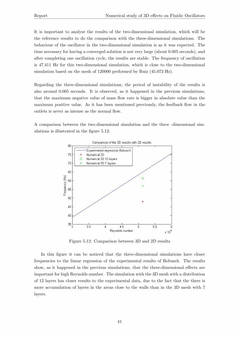
5.12 Comparison between 3D and 2D results . . . . . . . . . . . . . . . . . . . . 41
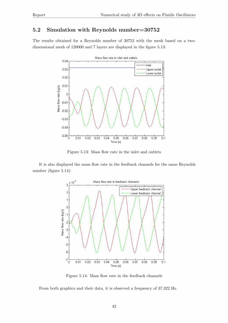
5.13 Mass flow rate in the inlet and outlets . . . . . . . . . . . . . . . . . . . . . 42
5.14 Mass flow rate in the feedback channels . . . . . . . . . . . . . . . . . . . . 42
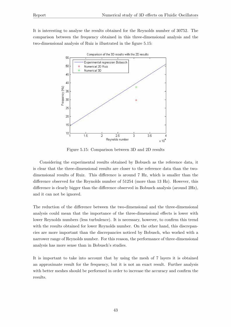
5.15 Comparison between 3D and 2D results . . . . . . . . . . . . . . . . . . . . 43
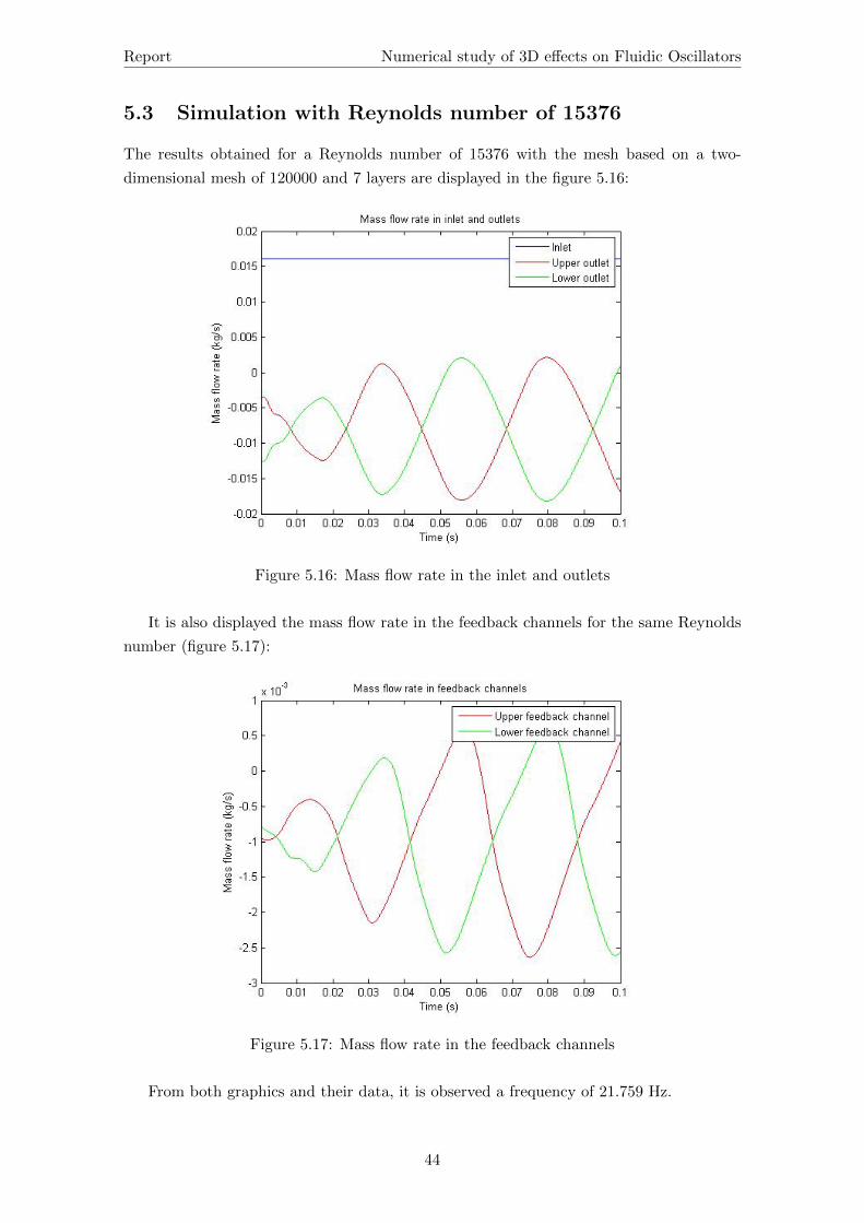
5.16 Mass flow rate in the inlet and outlets . . . . . . . . . . . . . . . . . . . . . 44
5.17 Mass flow rate in the feedback channels . . . . . . . . . . . . . . . . . . . . 44
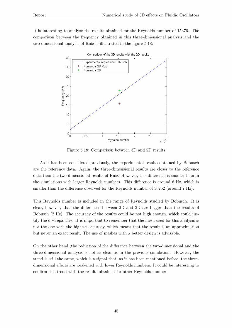
5.18 Comparison between 3D and 2D results . . . . . . . . . . . . . . . . . . . . 45
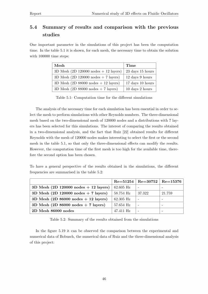
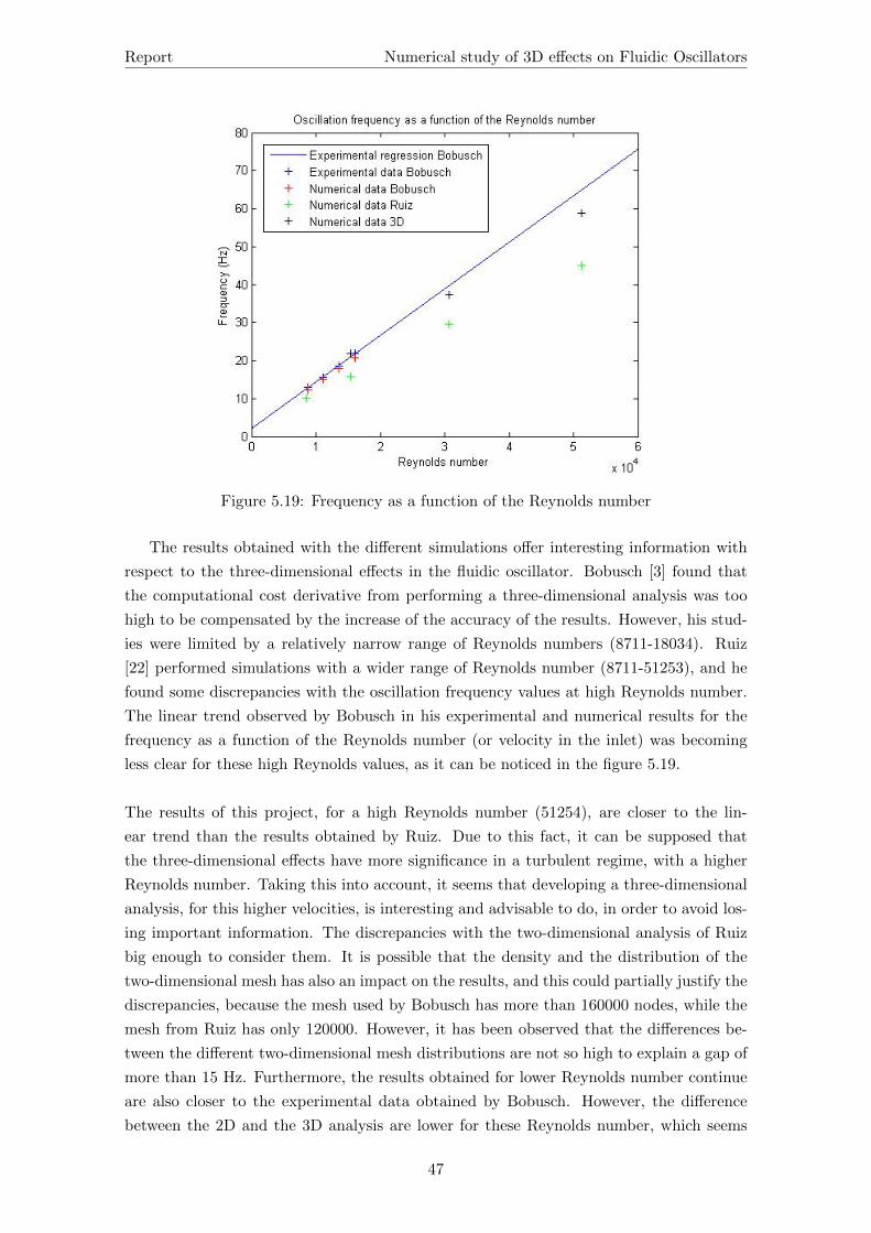
5.19 Frequency as a function of the Reynolds number . . . . . . . . . . . . . . . 47
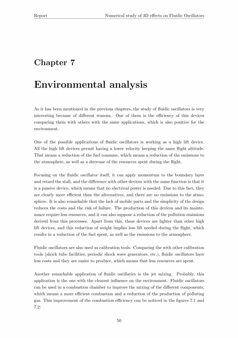
7.1 Concentrations of CO2 of the fluidic oscillator flame (a) and the plane-jet
flame (b) . . . . . . . . . . . . . . . . . . . . . . . . . . . . . . . . . . . . . 51
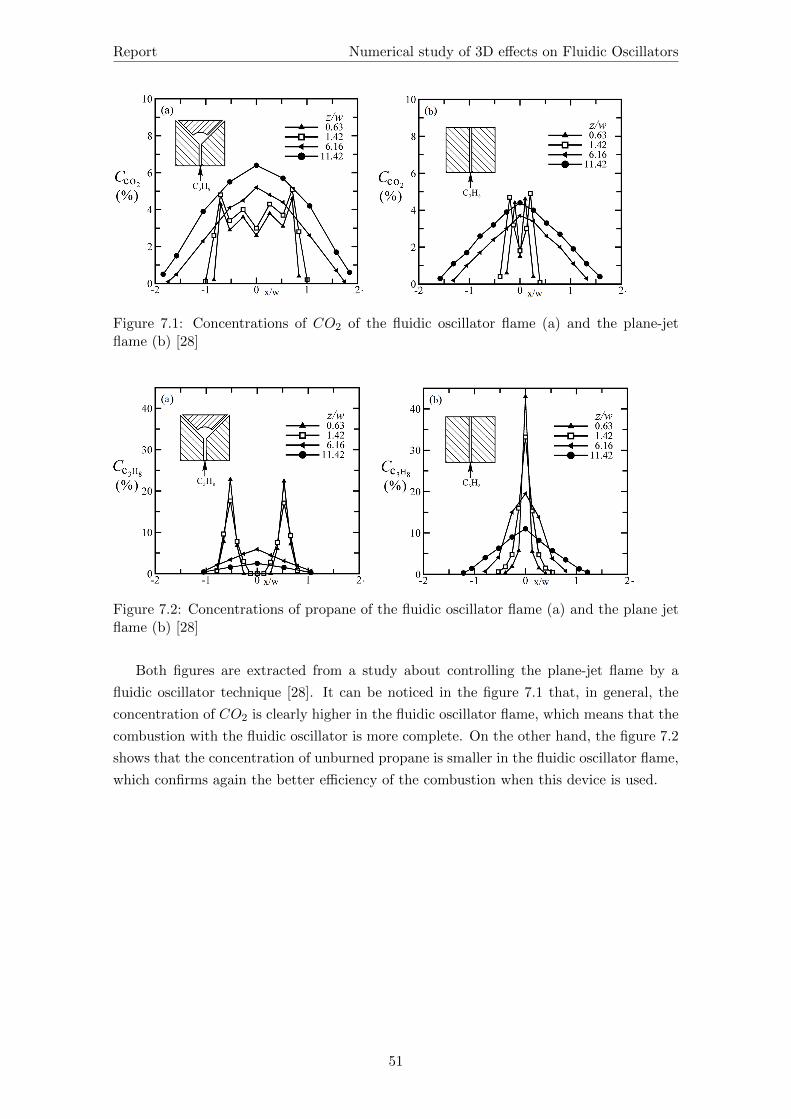
7.2 Concentrations of propane of the fluidic oscillator flame (a) and the plane
jet flame (b) . . . . . . . . . . . . . . . . . . . . . . . . . . . . . . . . . . . . 51
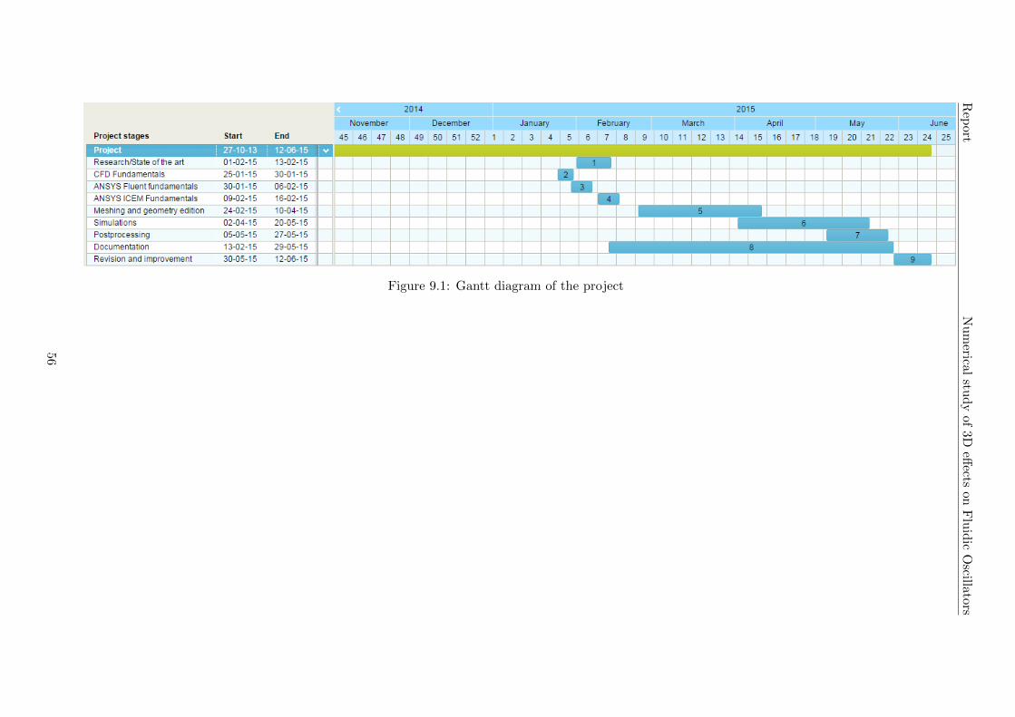
9.1 Gantt diagram of the project . . . . . . . . . . . . . . . . . . . . . . . . . . 56
v
Page 7
List of Tables
3.1 Summary of the experimental and numerical results obtained by Bobusch . 15
3.2 Numerical results obtained by Ruiz . . . . . . . . . . . . . . . . . . . . . . . 17
4.1 Computation time necessary for the simulations of Ruiz . . . . . . . . . . . 21
4.2 Parameters selected for the simulations of this project . . . . . . . . . . . . 30
5.1 Computation time for the different simulations . . . . . . . . . . . . . . . . 46
5.2 Summary of the results obtained from the simulations . . . . . . . . . . . . 46
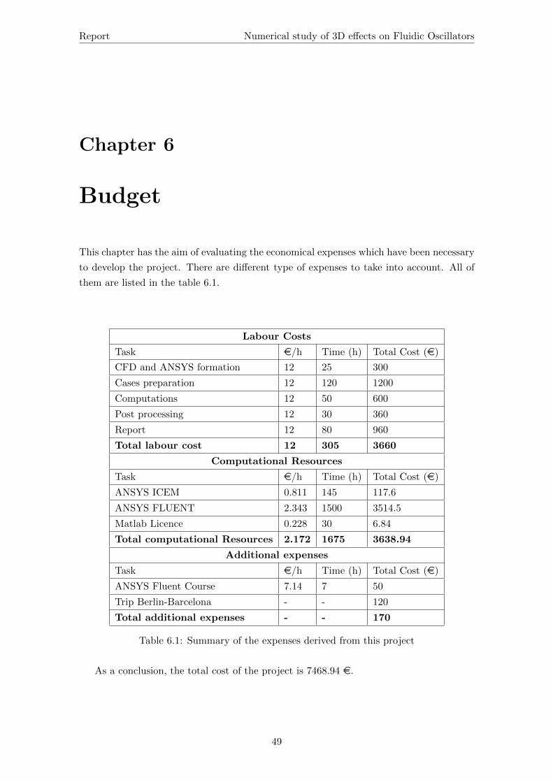
6.1 Summary of the expenses derived from this project . . . . . . . . . . . . . . 49
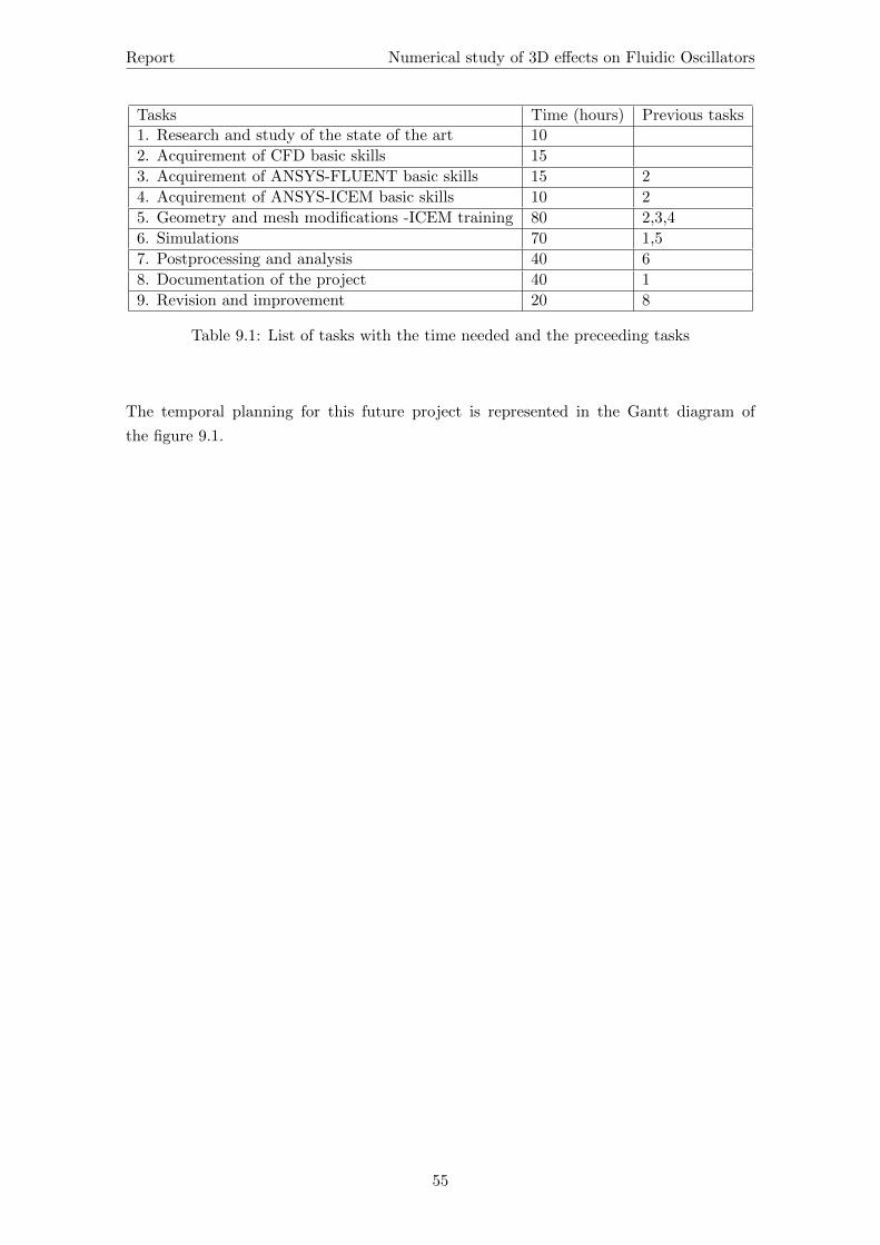
9.1 List of tasks with the time needed and the preceeding tasks . . . . . . . . . 55
vi
Page 8
Chapter 1
Introduction
1.1 Aim
The aim of this project is to develop a three-dimensional simulation , by using computa-
tional fluid dynamics (CFD), of a fluidic oscillator studied previously by Bobusch [3] and
Ruiz [22] in order to analyse the significance of the three-dimensional effects in this device.
1.2 Scope
Fluidic oscillators are devices with a large number of possible future applications in the
aeronautical field, therefore it is interesting to the know more about them. In a previ-
ous project developed by Ruiz [22] in the UPC (Universitat Politecnica de Catalunya), a
two-dimensional numerical simulation based on a reference fluidic oscillator was performed
in order to have a good approach to the numerical and experimental analysis developed
by Bobusch [4] [3] in the Technische Universitat Berlin, based on the same fluidic oscillator.
Ruiz found a slight difference between his results and the results obtained in the TU
Berlin, and one of the possible reasons for these discrepancies is not taking into account
the three-dimensional effects. This project is focused on studying the significance of these
effects. In order to achieve the goal of the project, it is previously necessary to acquire some
knowledge of fluidic oscillators, as well as knowledge of CFD, focusing on the tools ANSYS
Fluent and ANSYS ICEM. After these previous tasks, the main part of the project can
be developed. The tasks and activities necessary to carry out the project are enumerated
in the following list:
• Documentation about fluidic oscillators and study of the state of the art
• Acquirement of knowledge of CFD theorry and the the CFD tools ANSYS Fluent
and ANSYS ICEM
• Three-dimensional mesh construction and case preparation
• Three-dimensional simulation of the reference fluidic oscillator
1
Page 9
Report Numerical study of 3D effects on Fluidic Oscillators
• Comparison between the three-dimensional and the two-dimensional analysis of the
reference oscillator
• Enhancement, if possible, of the two-dimensional mesh to study the behaviour at
high Reynolds number, and comparison with the original results
1.3 Requirements
The requirements of this project are the following:
• Three-dimensional simulation of the fluidic oscillator studied in the TU Berlin by
Bobusch [3] [4] and in the UPC by Ruiz [22]
• Mesh construction by using the program ANSYS ICEM
• Simulation performed with the program ANSYS Fluent, using a Pressure-Based
solver, and treating the turbulence with the RANS equations and a SST turbulent
model
• Discussion of the results obtained with the three-dimensional analysis, and subse-
quent comparison with the numerical and experimental results of Bobusch, as well
as with the two-dimensional results of Ruiz
• Delivery of the project the 12nd of June
1.4 Justification
The study of fluidic oscillators began 50 years ago, but despite the fact that several studies
about them have been developed, there is still nowadays a certain lack of global knowl-
edge about fluidic oscillators. For this reason, it is a very interesting field of study. Some
applications with them are being currently performed, but it is not easy to know with
exactitude the potential range of applications of these devices.
Fluidic oscillators have applications in the aeronautical field. A fluidic oscillator is a
high lift device which participates in the control of the boundary layer: by applying mo-
mentum to the boundary layer, the stall can be retarded, which is especially interesting
during the take-off and landing of an aircraft. The basic advantage of fluidic oscillators
with respect to other high lift devices is the absence of mobile parts, which reduces the
complexity of the design, the costs and the risk of failure. Electrical power is not needed
(it is a passive high lift device), which is clearly efficient, the required mass flux is not
high, and they can operate under a great range of conditions. The main disadvantage is
that it is necessary to obtain certain entrance conditions in order to obtain the desired
exit conditions.
The results of the two-dimensional simulation developed by Ruiz were quite similar to
2
Page 10
Report Numerical study of 3D effects on Fluidic Oscillators
the results obtained by Bobusch. However, it has been noticed a slight difference be-
tween both studies in the values of the frequency as a function of the Reynolds number.
This difference, which is relatively small along a certain range of Reynolds number, could
be explained by not taking into account the three-dimensional effects. This possibility
justifies the interest of analysing how important can be these effects in fluidic oscillators,
and it is the main reason for the three-dimensional study which is developed in this project.
Furthermore, Ruiz has found that the linear trend of the oscillation frequency as function
of the Reynolds number is less clear for high Reynolds numbers. It is possible that this
behaviour is real at high Reynolds number, because the three-dimensional effects may be
more significant in a turbulent regime. However, another possibility is the density and
the distribution of the mesh built by Ruiz, which could produce some inaccurate results.
A secondary approach of this project could be, if possible, refining the two-dimensional
mesh of Ruiz in order to have a closer result to the experimental results of Bobusch in
high Reynolds number regimes.
1.5 State of the art
The fluidic oscillator is a device with no moving part which produces an oscillating jet
when it receives a fluid at a certain pressure, due to fluid-dynamic interactions. The high
range of frequencies it can operate at and the fact that it is a passive device are reasons
that justify the considerable amount of applications that it has.
The first fluidic oscillators were developed in the 1960’s, as a result of the research in
fluidic amplifiers. The fluidic oscillator has its roots based on the field of fluid logic, as it
is detailed by Morris [15], Kirshner and Katz [12]. An overview of the fluid amplifier tech-
nology can be found in the NASA contractor reports (Raber and Shinn [16] [17]). Fluid
logic principles were first applied by Spyropoulos [26] in order to develop a self-oscillating
fluid device, and Viets [27] also published work related with the development of fluidic
oscillators.
Regarding the recent studies, it is essential to highlight the amount of prior work to
characterize the flow of fluidic oscillators, specially focused on miniature fluidic oscilla-
tors. A characterization of miniature fluidic oscillators as possible devices for flow control
applications has been developed by Raman et al. [21] and Raghu et al. [20] . With the
same aim, Sakaue et al. [24] and Gregory et al. [23] have used pressure-sensitive paint
(PSP).
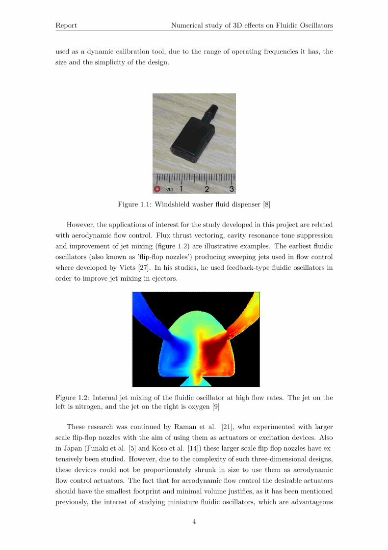
Since the first studies in the 1960’s, fluidic oscillators have been used for different ap-
plications. It is necessary to highlight the use of these devices as windshield washer fluid
dispensers (showed in figure 1.1) on automobiles: more than 45 million are produced every
year. Apart from this application, they have also been used to measure flow-rates, due to
the fact that the operating frequency is directly related to the flow rate. They can also be
3
Page 11
Report Numerical study of 3D effects on Fluidic Oscillators
used as a dynamic calibration tool, due to the range of operating frequencies it has, the
size and the simplicity of the design.
Figure 1.1: Windshield washer fluid dispenser [8]
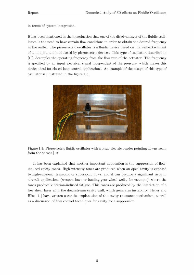
However, the applications of interest for the study developed in this project are related
with aerodynamic flow control. Flux thrust vectoring, cavity resonance tone suppression
and improvement of jet mixing (figure 1.2) are illustrative examples. The earliest fluidic
oscillators (also known as ’flip-flop nozzles’) producing sweeping jets used in flow control
where developed by Viets [27]. In his studies, he used feedback-type fluidic oscillators in
order to improve jet mixing in ejectors.
Figure 1.2: Internal jet mixing of the fluidic oscillator at high flow rates. The jet on theleft is nitrogen, and the jet on the right is oxygen [9]
These research was continued by Raman et al. [21], who experimented with larger
scale flip-flop nozzles with the aim of using them as actuators or excitation devices. Also
in Japan (Funaki et al. [5] and Koso et al. [14]) these larger scale flip-flop nozzles have ex-
tensively been studied. However, due to the complexity of such three-dimensional designs,
these devices could not be proportionately shrunk in size to use them as aerodynamic
flow control actuators. The fact that for aerodynamic flow control the desirable actuators
should have the smallest footprint and minimal volume justifies, as it has been mentioned
previously, the interest of studying miniature fluidic oscillators, which are advantageous
4
Page 12
Report Numerical study of 3D effects on Fluidic Oscillators
in terms of system integration.
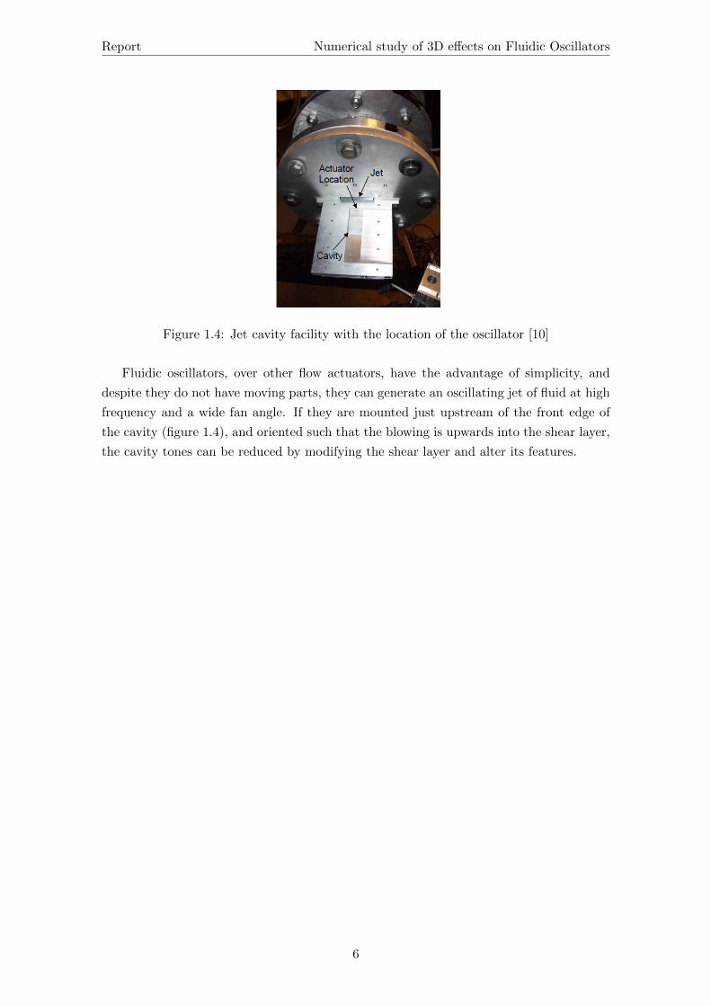
It has been mentioned in the introduction that one of the disadvantages of the fluidic oscil-
lators is the need to have certain flow conditions in order to obtain the desired frequency
in the outlet. The piezoelectric oscillator is a fluidic device based on the wall-attachment
of a fluid jet, and modulated by piezoelectric devices. This type of oscillator, described in
[10], decouples the operating frequency from the flow rate of the actuator. The frequency
is specified by an input electrical signal independent of the pressure, which makes this
device ideal for closed-loop control applications. An example of the design of this type of
oscillator is illustrated in the figure 1.3.
Figure 1.3: Piezoelectric fluidic oscillator with a piezo-electric bender pointing downstreamfrom the throat [10]
It has been explained that another important application is the suppression of flow-
induced cavity tones. High intensity tones are produced when an open cavity is exposed
to high-subsonic, transonic or supersonic flows, and it can become a significant issue in
aircraft applications (weapon bays or landing-gear wheel wells, for example), where the
tones produce vibration-induced fatigue. This tones are produced by the interaction of a
free shear layer with the downstream cavity wall, which generates instability. Heller and
Bliss [11] have written a concise explanation of the cavity resonance mechanism, as well
as a discussion of flow control techniques for cavity tone suppression.
5
Page 13
Report Numerical study of 3D effects on Fluidic Oscillators
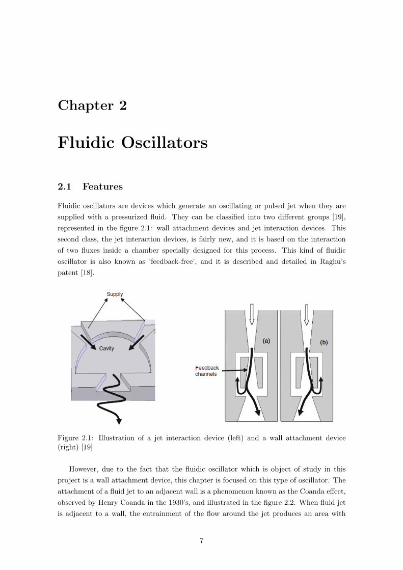
Figure 1.4: Jet cavity facility with the location of the oscillator [10]
Fluidic oscillators, over other flow actuators, have the advantage of simplicity, and
despite they do not have moving parts, they can generate an oscillating jet of fluid at high
frequency and a wide fan angle. If they are mounted just upstream of the front edge of
the cavity (figure 1.4), and oriented such that the blowing is upwards into the shear layer,
the cavity tones can be reduced by modifying the shear layer and alter its features.
6
Page 14
Chapter 2
Fluidic Oscillators
2.1 Features
Fluidic oscillators are devices which generate an oscillating or pulsed jet when they are
supplied with a pressurized fluid. They can be classified into two different groups [19],
represented in the figure 2.1: wall attachment devices and jet interaction devices. This
second class, the jet interaction devices, is fairly new, and it is based on the interaction
of two fluxes inside a chamber specially designed for this process. This kind of fluidic
oscillator is also known as ’feedback-free’, and it is described and detailed in Raghu’s
patent [18].
Figure 2.1: Illustration of a jet interaction device (left) and a wall attachment device(right) [19]
However, due to the fact that the fluidic oscillator which is object of study in this
project is a wall attachment device, this chapter is focused on this type of oscillator. The
attachment of a fluid jet to an adjacent wall is a phenomenon known as the Coanda effect,
observed by Henry Coanda in the 1930’s, and illustrated in the figure 2.2. When fluid jet
is adjacent to a wall, the entrainment of the flow around the jet produces an area with
7
Page 15
Report Numerical study of 3D effects on Fluidic Oscillators
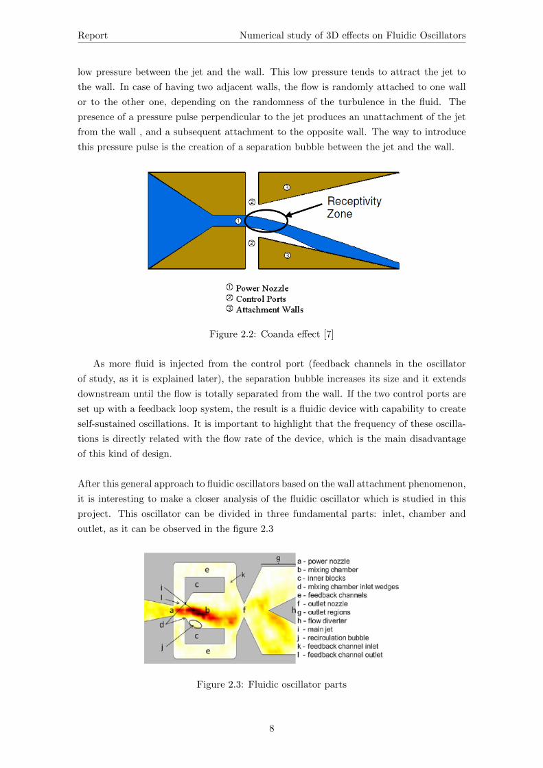
low pressure between the jet and the wall. This low pressure tends to attract the jet to
the wall. In case of having two adjacent walls, the flow is randomly attached to one wall
or to the other one, depending on the randomness of the turbulence in the fluid. The
presence of a pressure pulse perpendicular to the jet produces an unattachment of the jet
from the wall , and a subsequent attachment to the opposite wall. The way to introduce
this pressure pulse is the creation of a separation bubble between the jet and the wall.
Figure 2.2: Coanda effect [7]
As more fluid is injected from the control port (feedback channels in the oscillator
of study, as it is explained later), the separation bubble increases its size and it extends
downstream until the flow is totally separated from the wall. If the two control ports are
set up with a feedback loop system, the result is a fluidic device with capability to create
self-sustained oscillations. It is important to highlight that the frequency of these oscilla-
tions is directly related with the flow rate of the device, which is the main disadvantage
of this kind of design.
After this general approach to fluidic oscillators based on the wall attachment phenomenon,
it is interesting to make a closer analysis of the fluidic oscillator which is studied in this
project. This oscillator can be divided in three fundamental parts: inlet, chamber and
outlet, as it can be observed in the figure 2.3
Figure 2.3: Fluidic oscillator parts
8
Page 16
Report Numerical study of 3D effects on Fluidic Oscillators
The inlet is the longest part of the device. The big length of the inlet and its shape
have been designed to achieve the most uniform and constant flux possible before the
fluid arrives to the mixing chamber. It is desirable to obtain a longitudinal flux to avoid
perturbations on the jet inside the mixing chamber. The chamber is located between
the inlet and the outlet, and it is the area where the characteristic processes of fluidic
oscillators happen. The chamber has a mixing area where the Coanda effect happens, and
two feedback channels which are necessary to have a feedback loop system which allows
the device to create self-sustained oscillations, as it has been mentioned before. Finally,
the outlet is located after the mixing chamber, and it is divided in two exit nozzles. The
jet oscillates between these two nozzles, which are separated by a deviator. The nozzles
accelerate the fluid until the exit conditions are achieved.
2.2 Performance
In the previous section it has been explained the general performance of the wall attach-
ment fluidic oscillators. It is interesting, however,to adapt the explanation to the fluidic
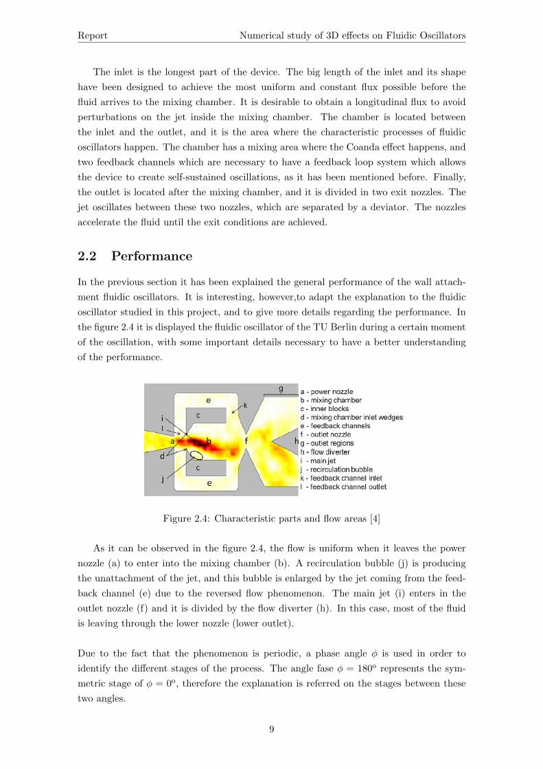
oscillator studied in this project, and to give more details regarding the performance. In
the figure 2.4 it is displayed the fluidic oscillator of the TU Berlin during a certain moment
of the oscillation, with some important details necessary to have a better understanding
of the performance.
Figure 2.4: Characteristic parts and flow areas [4]
As it can be observed in the figure 2.4, the flow is uniform when it leaves the power
nozzle (a) to enter into the mixing chamber (b). A recirculation bubble (j) is producing
the unattachment of the jet, and this bubble is enlarged by the jet coming from the feed-
back channel (e) due to the reversed flow phenomenon. The main jet (i) enters in the
outlet nozzle (f) and it is divided by the flow diverter (h). In this case, most of the fluid
is leaving through the lower nozzle (lower outlet).
Due to the fact that the phenomenon is periodic, a phase angle φ is used in order to
identify the different stages of the process. The angle fase φ = 180o represents the sym-
metric stage of φ = 0o, therefore the explanation is referred on the stages between these
two angles.
9
Page 17
Report Numerical study of 3D effects on Fluidic Oscillators
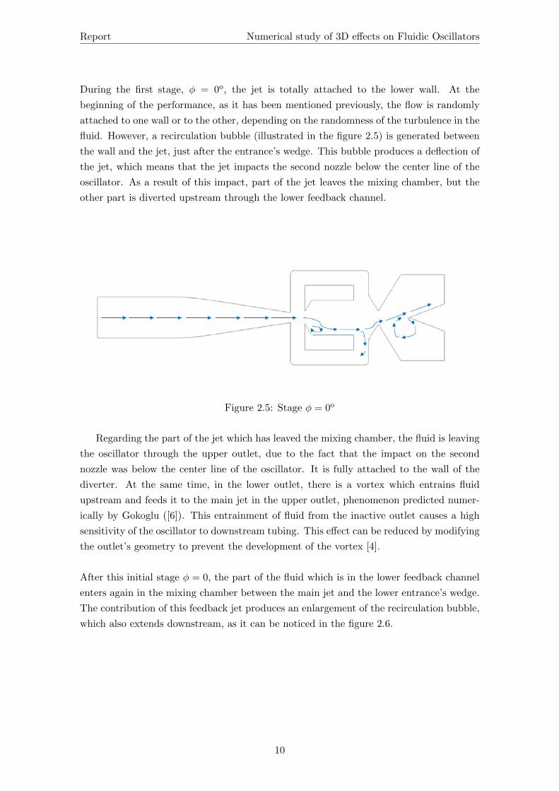
During the first stage, φ = 0o, the jet is totally attached to the lower wall. At the
beginning of the performance, as it has been mentioned previously, the flow is randomly
attached to one wall or to the other, depending on the randomness of the turbulence in the
fluid. However, a recirculation bubble (illustrated in the figure 2.5) is generated between
the wall and the jet, just after the entrance’s wedge. This bubble produces a deflection of
the jet, which means that the jet impacts the second nozzle below the center line of the
oscillator. As a result of this impact, part of the jet leaves the mixing chamber, but the
other part is diverted upstream through the lower feedback channel.
Figure 2.5: Stage φ = 0o
Regarding the part of the jet which has leaved the mixing chamber, the fluid is leaving
the oscillator through the upper outlet, due to the fact that the impact on the second
nozzle was below the center line of the oscillator. It is fully attached to the wall of the
diverter. At the same time, in the lower outlet, there is a vortex which entrains fluid
upstream and feeds it to the main jet in the upper outlet, phenomenon predicted numer-
ically by Gokoglu ([6]). This entrainment of fluid from the inactive outlet causes a high
sensitivity of the oscillator to downstream tubing. This effect can be reduced by modifying
the outlet’s geometry to prevent the development of the vortex [4].
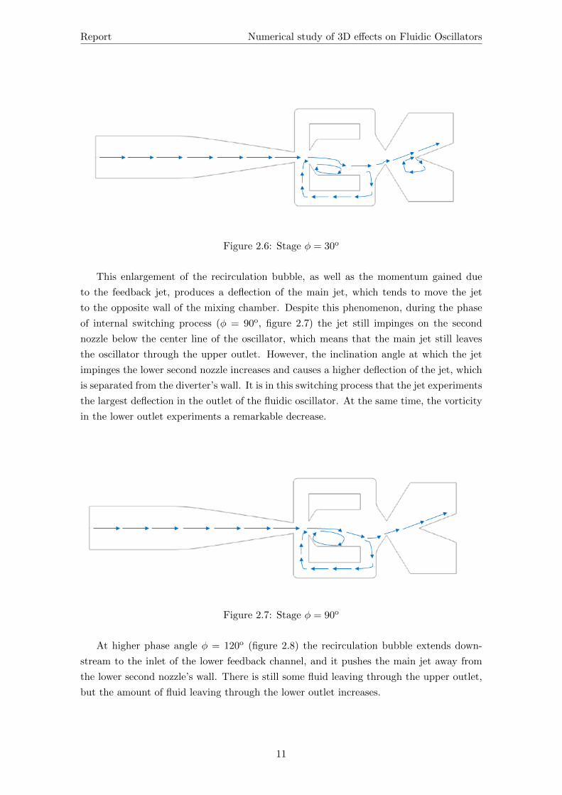
After this initial stage φ = 0, the part of the fluid which is in the lower feedback channel
enters again in the mixing chamber between the main jet and the lower entrance’s wedge.
The contribution of this feedback jet produces an enlargement of the recirculation bubble,
which also extends downstream, as it can be noticed in the figure 2.6.
10
Page 18
Report Numerical study of 3D effects on Fluidic Oscillators
Figure 2.6: Stage φ = 30o
This enlargement of the recirculation bubble, as well as the momentum gained due
to the feedback jet, produces a deflection of the main jet, which tends to move the jet
to the opposite wall of the mixing chamber. Despite this phenomenon, during the phase
of internal switching process (φ = 90o, figure 2.7) the jet still impinges on the second
nozzle below the center line of the oscillator, which means that the main jet still leaves
the oscillator through the upper outlet. However, the inclination angle at which the jet
impinges the lower second nozzle increases and causes a higher deflection of the jet, which
is separated from the diverter’s wall. It is in this switching process that the jet experiments
the largest deflection in the outlet of the fluidic oscillator. At the same time, the vorticity
in the lower outlet experiments a remarkable decrease.
Figure 2.7: Stage φ = 90o
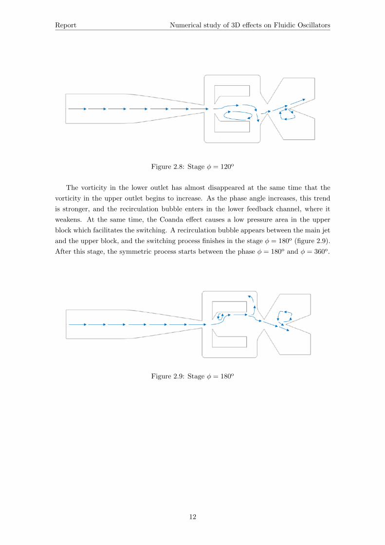
At higher phase angle φ = 120o (figure 2.8) the recirculation bubble extends down-
stream to the inlet of the lower feedback channel, and it pushes the main jet away from
the lower second nozzle’s wall. There is still some fluid leaving through the upper outlet,
but the amount of fluid leaving through the lower outlet increases.
11
Page 19
Report Numerical study of 3D effects on Fluidic Oscillators
Figure 2.8: Stage φ = 120o
The vorticity in the lower outlet has almost disappeared at the same time that the
vorticity in the upper outlet begins to increase. As the phase angle increases, this trend
is stronger, and the recirculation bubble enters in the lower feedback channel, where it
weakens. At the same time, the Coanda effect causes a low pressure area in the upper
block which facilitates the switching. A recirculation bubble appears between the main jet
and the upper block, and the switching process finishes in the stage φ = 180o (figure 2.9).
After this stage, the symmetric process starts between the phase φ = 180o and φ = 360o.
Figure 2.9: Stage φ = 180o
12
Page 20
Report Numerical study of 3D effects on Fluidic Oscillators
Chapter 3
Previous studies with the same
oscillator
This project is focused on a three-dimensional numerical simulation based on a concrete
fluidic oscillator. In order to have a better understanding of the context of this project,
it is interesting to explain the previous experimental and numerical studies based on this
oscillator.
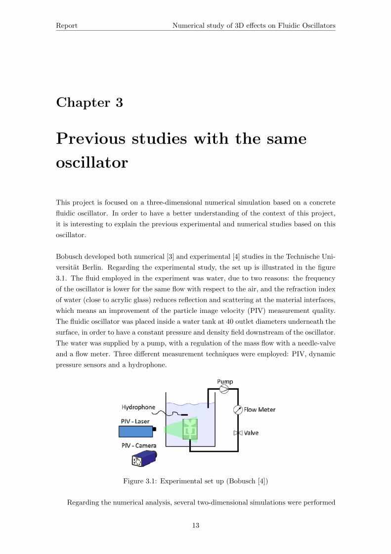
Bobusch developed both numerical [3] and experimental [4] studies in the Technische Uni-
versitat Berlin. Regarding the experimental study, the set up is illustrated in the figure
3.1. The fluid employed in the experiment was water, due to two reasons: the frequency
of the oscillator is lower for the same flow with respect to the air, and the refraction index
of water (close to acrylic glass) reduces reflection and scattering at the material interfaces,
which means an improvement of the particle image velocity (PIV) measurement quality.
The fluidic oscillator was placed inside a water tank at 40 outlet diameters underneath the
surface, in order to have a constant pressure and density field downstream of the oscillator.
The water was supplied by a pump, with a regulation of the mass flow with a needle-valve
and a flow meter. Three different measurement techniques were employed: PIV, dynamic
pressure sensors and a hydrophone.
Figure 3.1: Experimental set up (Bobusch [4])
Regarding the numerical analysis, several two-dimensional simulations were performed
13
Page 21
Report Numerical study of 3D effects on Fluidic Oscillators
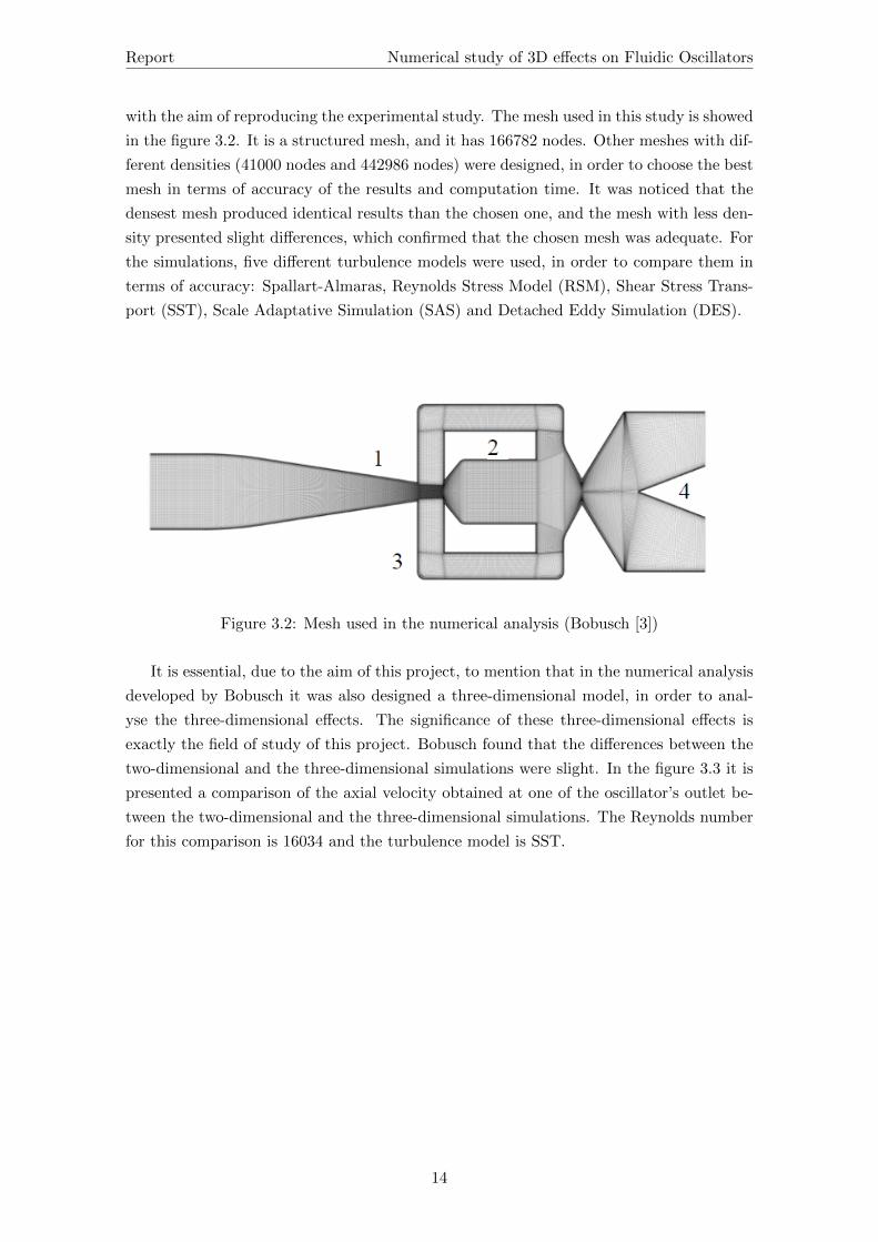
with the aim of reproducing the experimental study. The mesh used in this study is showed
in the figure 3.2. It is a structured mesh, and it has 166782 nodes. Other meshes with dif-
ferent densities (41000 nodes and 442986 nodes) were designed, in order to choose the best
mesh in terms of accuracy of the results and computation time. It was noticed that the
densest mesh produced identical results than the chosen one, and the mesh with less den-
sity presented slight differences, which confirmed that the chosen mesh was adequate. For
the simulations, five different turbulence models were used, in order to compare them in
terms of accuracy: Spallart-Almaras, Reynolds Stress Model (RSM), Shear Stress Trans-
port (SST), Scale Adaptative Simulation (SAS) and Detached Eddy Simulation (DES).
Figure 3.2: Mesh used in the numerical analysis (Bobusch [3])
It is essential, due to the aim of this project, to mention that in the numerical analysis
developed by Bobusch it was also designed a three-dimensional model, in order to anal-
yse the three-dimensional effects. The significance of these three-dimensional effects is
exactly the field of study of this project. Bobusch found that the differences between the
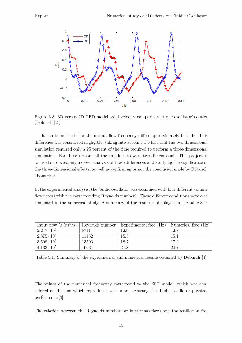
two-dimensional and the three-dimensional simulations were slight. In the figure 3.3 it is
presented a comparison of the axial velocity obtained at one of the oscillator’s outlet be-
tween the two-dimensional and the three-dimensional simulations. The Reynolds number
for this comparison is 16034 and the turbulence model is SST.
14
Page 22
Report Numerical study of 3D effects on Fluidic Oscillators
Figure 3.3: 3D versus 2D CFD model axial velocity comparison at one oscillator’s outlet(Bobusch [2])
It can be noticed that the output flow frequency differs approximately in 2 Hz. This
difference was considered negligible, taking into account the fact that the two-dimensional
simulation required only a 25 percent of the time required to perform a three-dimensional
simulation. For these reason, all the simulations were two-dimensional. This project is
focused on developing a closer analysis of these differences and studying the significance of
the three-dimensional effects, as well as confirming or not the conclusion made by Bobusch
about that.
In the experimental analysis, the fluidic oscillator was examined with four different volume
flow rates (with the corresponding Reynolds number). These different conditions were also
simulated in the numerical study. A summary of the results is displayed in the table 3.1:
Input flow Q (m3/s) Reynolds number Experimental freq (Hz) Numerical freq (Hz)2.247 · 105 8711 12.9 12.3
2.875 · 105 11152 15.5 15.1
3.508 · 105 13593 18.7 17.9
4.133 · 105 16034 21.8 20.7
Table 3.1: Summary of the experimental and numerical results obtained by Bobusch [4]
The values of the numerical frequency correspond to the SST model, which was con-
sidered as the one which reproduces with more accuracy the fluidic oscillator physical
performance[3].
The relation between the Reynolds number (or inlet mass flow) and the oscillation fre-
15
Page 23
Report Numerical study of 3D effects on Fluidic Oscillators
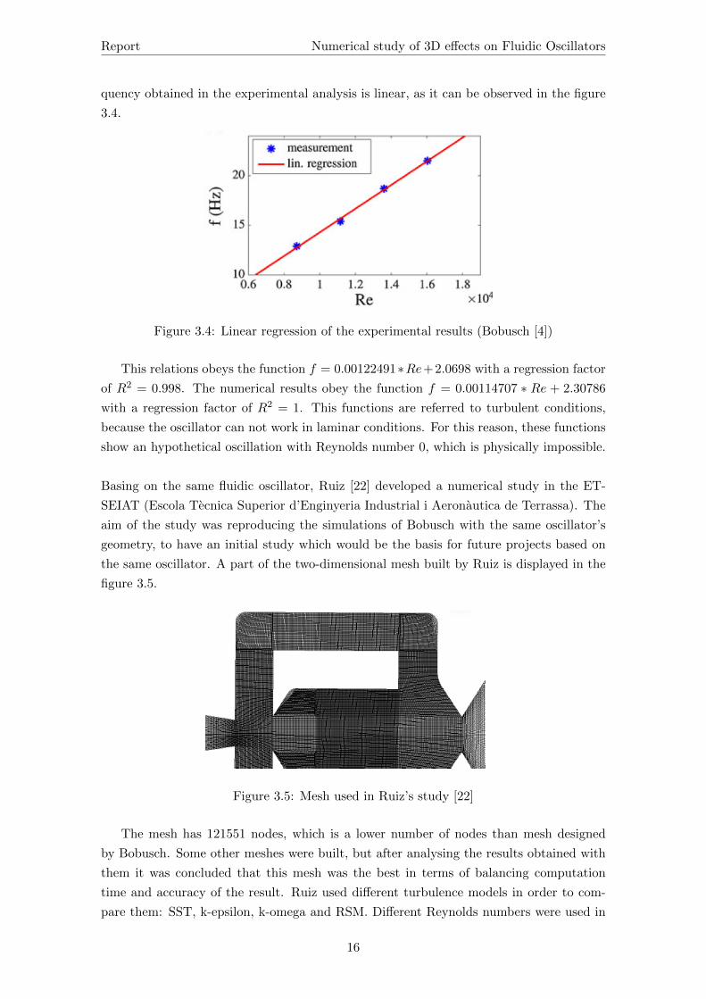
quency obtained in the experimental analysis is linear, as it can be observed in the figure
3.4.
Figure 3.4: Linear regression of the experimental results (Bobusch [4])
This relations obeys the function f = 0.00122491∗Re+2.0698 with a regression factor
of R2 = 0.998. The numerical results obey the function f = 0.00114707 ∗ Re + 2.30786
with a regression factor of R2 = 1. This functions are referred to turbulent conditions,
because the oscillator can not work in laminar conditions. For this reason, these functions
show an hypothetical oscillation with Reynolds number 0, which is physically impossible.
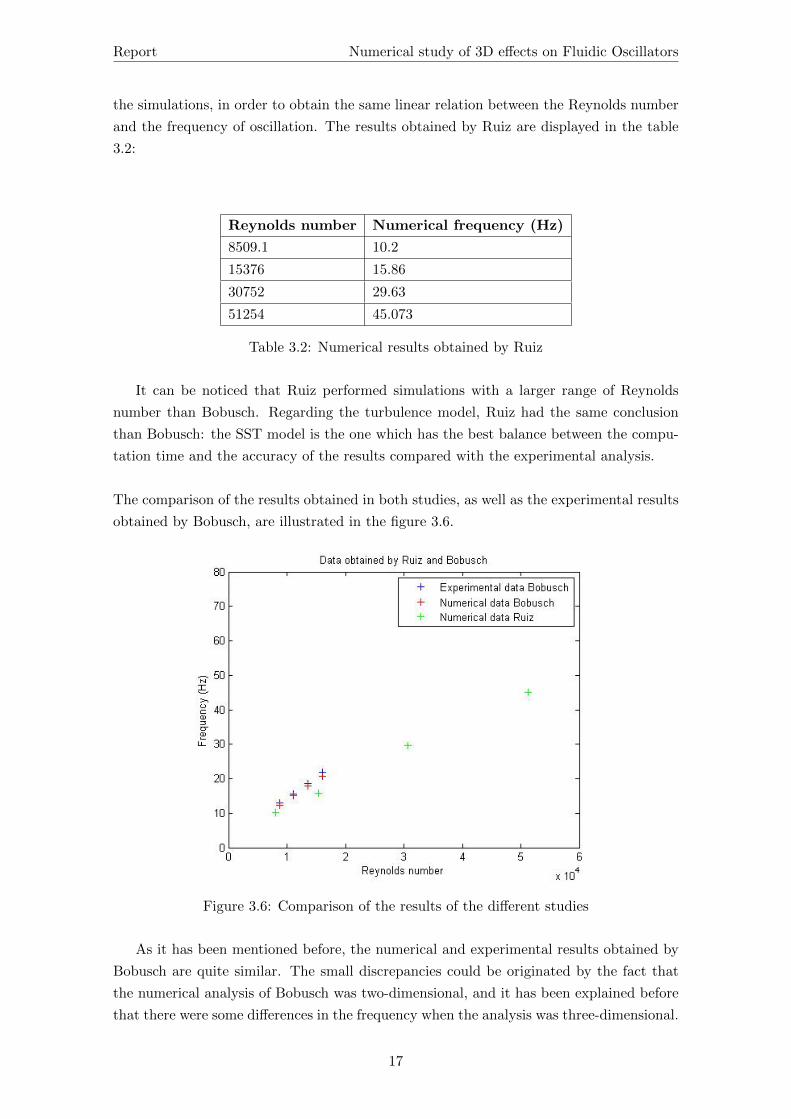
Basing on the same fluidic oscillator, Ruiz [22] developed a numerical study in the ET-
SEIAT (Escola Tecnica Superior d’Enginyeria Industrial i Aeronautica de Terrassa). The
aim of the study was reproducing the simulations of Bobusch with the same oscillator’s
geometry, to have an initial study which would be the basis for future projects based on
the same oscillator. A part of the two-dimensional mesh built by Ruiz is displayed in the
figure 3.5.
Figure 3.5: Mesh used in Ruiz’s study [22]
The mesh has 121551 nodes, which is a lower number of nodes than mesh designed
by Bobusch. Some other meshes were built, but after analysing the results obtained with
them it was concluded that this mesh was the best in terms of balancing computation
time and accuracy of the result. Ruiz used different turbulence models in order to com-
pare them: SST, k-epsilon, k-omega and RSM. Different Reynolds numbers were used in
16
Page 24
Report Numerical study of 3D effects on Fluidic Oscillators
the simulations, in order to obtain the same linear relation between the Reynolds number
and the frequency of oscillation. The results obtained by Ruiz are displayed in the table
3.2:
Reynolds number Numerical frequency (Hz)
8509.1 10.2
15376 15.86
30752 29.63
51254 45.073
Table 3.2: Numerical results obtained by Ruiz
It can be noticed that Ruiz performed simulations with a larger range of Reynolds
number than Bobusch. Regarding the turbulence model, Ruiz had the same conclusion
than Bobusch: the SST model is the one which has the best balance between the compu-
tation time and the accuracy of the results compared with the experimental analysis.
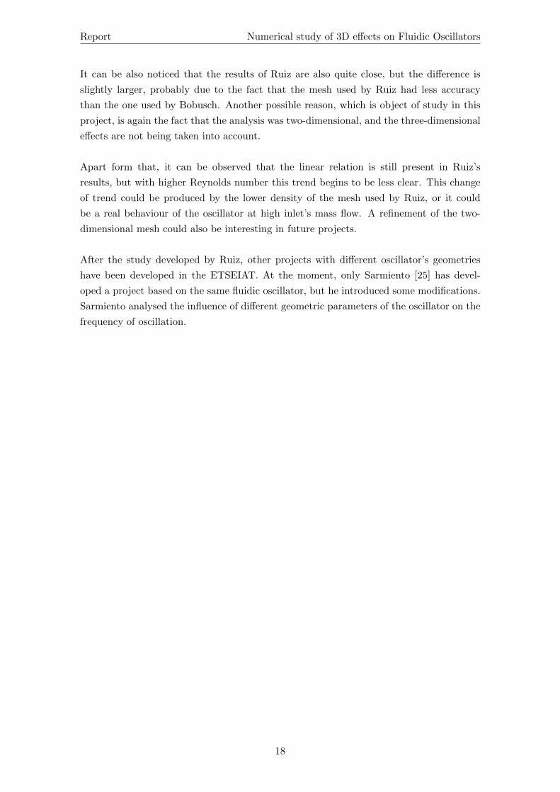
The comparison of the results obtained in both studies, as well as the experimental results
obtained by Bobusch, are illustrated in the figure 3.6.
Figure 3.6: Comparison of the results of the different studies
As it has been mentioned before, the numerical and experimental results obtained by
Bobusch are quite similar. The small discrepancies could be originated by the fact that
the numerical analysis of Bobusch was two-dimensional, and it has been explained before
that there were some differences in the frequency when the analysis was three-dimensional.
17
Page 25
Report Numerical study of 3D effects on Fluidic Oscillators
It can be also noticed that the results of Ruiz are also quite close, but the difference is
slightly larger, probably due to the fact that the mesh used by Ruiz had less accuracy
than the one used by Bobusch. Another possible reason, which is object of study in this
project, is again the fact that the analysis was two-dimensional, and the three-dimensional
effects are not being taken into account.
Apart form that, it can be observed that the linear relation is still present in Ruiz’s
results, but with higher Reynolds number this trend begins to be less clear. This change
of trend could be produced by the lower density of the mesh used by Ruiz, or it could
be a real behaviour of the oscillator at high inlet’s mass flow. A refinement of the two-
dimensional mesh could also be interesting in future projects.
After the study developed by Ruiz, other projects with different oscillator’s geometries
have been developed in the ETSEIAT. At the moment, only Sarmiento [25] has devel-
oped a project based on the same fluidic oscillator, but he introduced some modifications.
Sarmiento analysed the influence of different geometric parameters of the oscillator on the
frequency of oscillation.
18
Page 26
Report Numerical study of 3D effects on Fluidic Oscillators
Chapter 4
Computational study
4.1 Aim
The aim of the computational study of this project is simulating the reference fluidic os-
cillator with a three-dimensional mesh. The results of this simulation will be compared
with the results obtained by Ruiz [22] in his two-dimensional study, as well as with the
numerical [3] and the experimental [4] results obtained by Bobusch in the TU Berlin. The
interest of doing this study is analysing the significance of the three-dimensional effects
in this oscillator, and discussing if the differences observed are large enough to justify the
increase of computation time needed to perform the three-dimensional simulation.
To achieve this, the simulation has been developed with the same conditions than the
simulation performed by Ruiz, which was designed so that the simulation was a faith-
ful reproduction of Bobusch’s studies. The computational study has been developed by
using the tools ANSYS ICEM (for the design of the mesh) and ANSYS Fluent (for the
computations).
4.2 Meshing design
A good design of the mesh is essential to have the best approach possible to the real
experiment. A mesh is the discretization of the domain in cells in which the physical
equations of the problem are applied. The meshing has a direct impact on the accuracy
of the results and the computation time, so it is important to find a compromise solution,
specially in this project, because the time necessary for the computations could be very
high due to the large number of nodes, and this fact could be problematic to finish the
project before the established deadlines. As it has been mentioned previously, the tool
ANSYS ICEM has been used to design the mesh.
4.2.1 Two-dimensional mesh of reference
In order to compare the three-dimensional results obtained in this project with the re-
sults obtained in the two-dimensional study of Ruiz, the three-dimensional meshes used
19
Page 27
Report Numerical study of 3D effects on Fluidic Oscillators
are based on the two-dimensional meshes designed by Ruiz. The reference mesh is the
one selected by Ruiz as desirable, because he concluded that the accuracy is relatively
high and the computation time is not very big. This mesh is widely described in Ruiz’s
project [22], but there are some details which are important to highlight to have a better
understanding of the simulations.
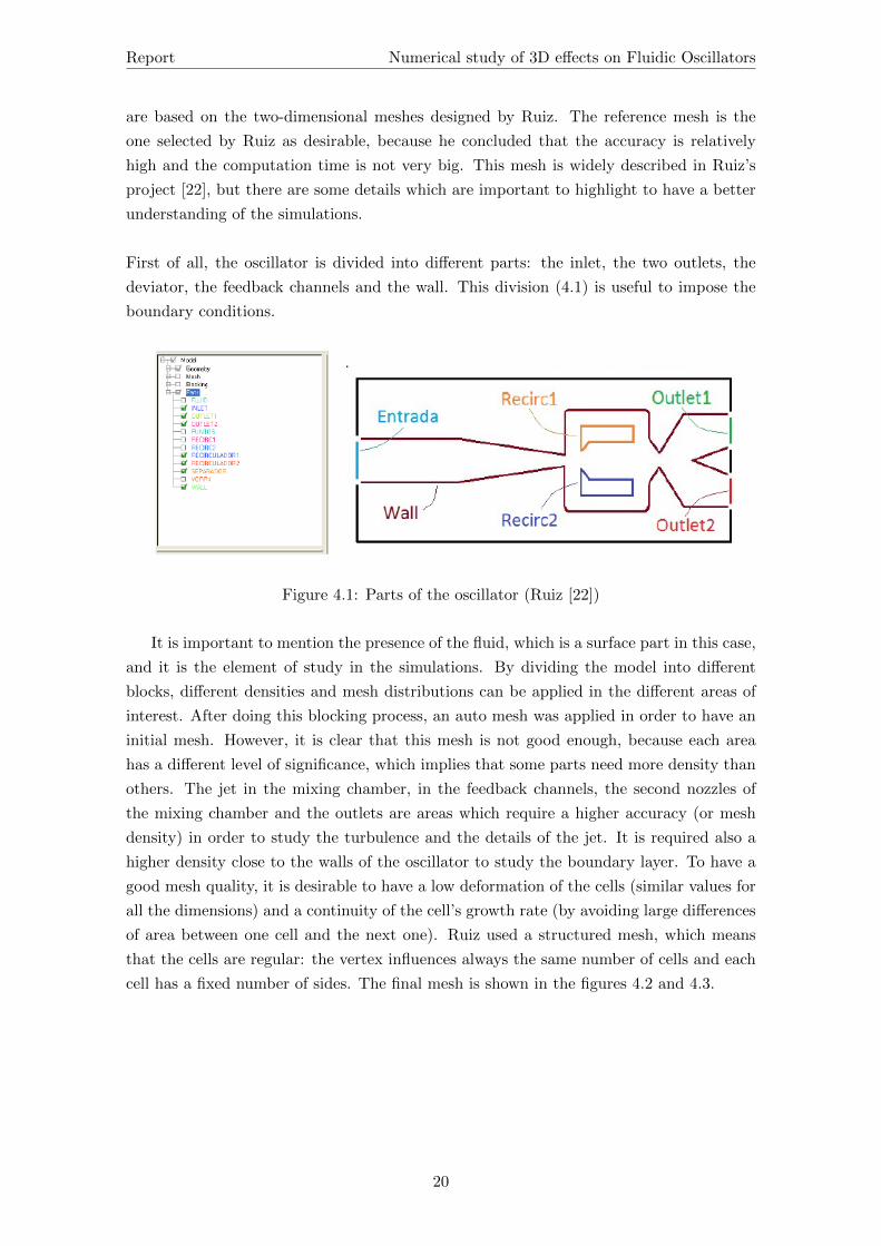
First of all, the oscillator is divided into different parts: the inlet, the two outlets, the
deviator, the feedback channels and the wall. This division (4.1) is useful to impose the
boundary conditions.
Figure 4.1: Parts of the oscillator (Ruiz [22])
It is important to mention the presence of the fluid, which is a surface part in this case,
and it is the element of study in the simulations. By dividing the model into different
blocks, different densities and mesh distributions can be applied in the different areas of
interest. After doing this blocking process, an auto mesh was applied in order to have an
initial mesh. However, it is clear that this mesh is not good enough, because each area
has a different level of significance, which implies that some parts need more density than
others. The jet in the mixing chamber, in the feedback channels, the second nozzles of
the mixing chamber and the outlets are areas which require a higher accuracy (or mesh
density) in order to study the turbulence and the details of the jet. It is required also a
higher density close to the walls of the oscillator to study the boundary layer. To have a
good mesh quality, it is desirable to have a low deformation of the cells (similar values for
all the dimensions) and a continuity of the cell’s growth rate (by avoiding large differences
of area between one cell and the next one). Ruiz used a structured mesh, which means
that the cells are regular: the vertex influences always the same number of cells and each
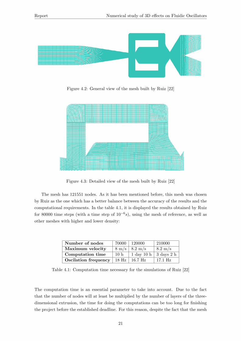
cell has a fixed number of sides. The final mesh is shown in the figures 4.2 and 4.3.
20
Page 28
Report Numerical study of 3D effects on Fluidic Oscillators
Figure 4.2: General view of the mesh built by Ruiz [22]
Figure 4.3: Detailed view of the mesh built by Ruiz [22]
The mesh has 121551 nodes. As it has been mentioned before, this mesh was chosen
by Ruiz as the one which has a better balance between the accuracy of the results and the
computational requirements. In the table 4.1, it is displayed the results obtained by Ruiz
for 80000 time steps (with a time step of 10−6s), using the mesh of reference, as well as
other meshes with higher and lower density:
Number of nodes 70000 120000 210000Maximum velocity 8 m/s 8.2 m/s 8.2 m/s
Computation time 10 h 1 day 10 h 3 days 2 h
Oscilation frequency 18 Hz 16.7 Hz 17.1 Hz
Table 4.1: Computation time necessary for the simulations of Ruiz [22]
The computation time is an essential parameter to take into account. Due to the fact
that the number of nodes will at least be multiplied by the number of layers of the three-
dimensional extrusion, the time for doing the computations can be too long for finishing
the project before the established deadline. For this reason, despite the fact that the mesh
21
Page 29
Report Numerical study of 3D effects on Fluidic Oscillators
with 210000 nodes presents more accuracy in the results, the mesh selected to work in this
project has been the one with 120000 nodes. This is the mesh which has been used as a
reference mesh for the three-dimensional simulation. It is important to highlight that the
significance of the three-dimensional effects can be analysed with the simulations even if
the two-dimensional mesh has not a very high accuracy.
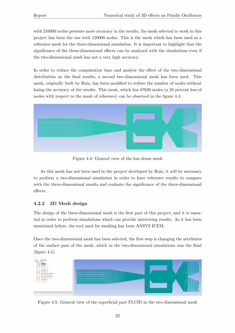
In order to reduce the computation time and analyse the effect of the two-dimensional
distribution on the final results, a second two-dimensional mesh has been used. This
mesh, originally built by Ruiz, has been modified to reduce the number of nodes without
losing the accuracy of the results. This mesh, which has 87630 nodes (a 28 percent less of
nodes with respect to the mesh of reference) can be observed in the figure 4.4:
Figure 4.4: General view of the less dense mesh
As this mesh has not been used in the project developed by Ruiz, it will be necessary
to perform a two-dimensional simulation in order to have reference results to compare
with the three-dimensional results and evaluate the significance of the three-dimensional
effects.
4.2.2 3D Mesh design
The design of the three-dimensional mesh is the first part of this project, and it is essen-
tial in order to perform simulations which can provide interesting results. As it has been
mentioned before, the tool used for meshing has been ANSYS ICEM.
Once the two-dimensional mesh has been selected, the first step is changing the attributes
of the surface part of the mesh, which in the two-dimensional simulations was the fluid
(figure 4.5).
Figure 4.5: General view of the superficial part FLUID in the two-dimensional mesh
22
Page 30
Report Numerical study of 3D effects on Fluidic Oscillators
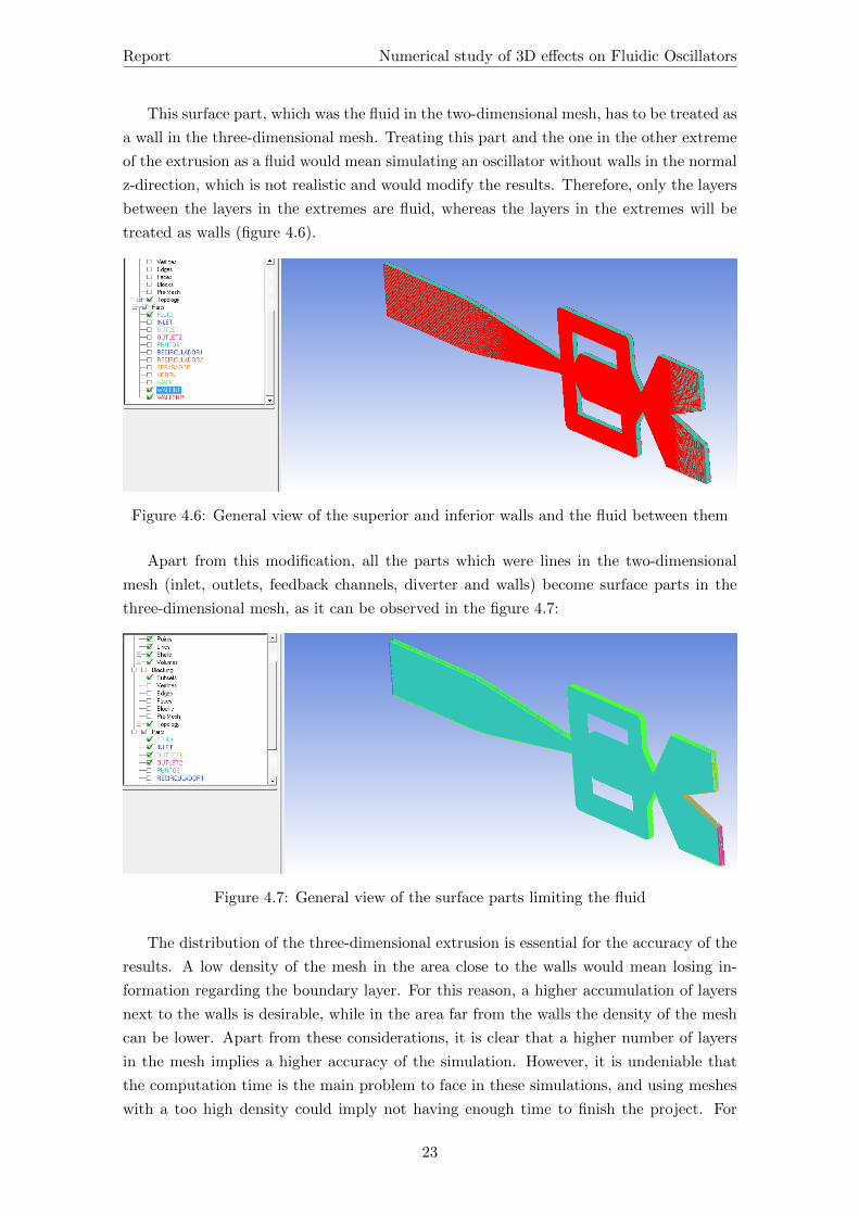
This surface part, which was the fluid in the two-dimensional mesh, has to be treated as
a wall in the three-dimensional mesh. Treating this part and the one in the other extreme
of the extrusion as a fluid would mean simulating an oscillator without walls in the normal
z-direction, which is not realistic and would modify the results. Therefore, only the layers
between the layers in the extremes are fluid, whereas the layers in the extremes will be
treated as walls (figure 4.6).
Figure 4.6: General view of the superior and inferior walls and the fluid between them
Apart from this modification, all the parts which were lines in the two-dimensional
mesh (inlet, outlets, feedback channels, diverter and walls) become surface parts in the
three-dimensional mesh, as it can be observed in the figure 4.7:
Figure 4.7: General view of the surface parts limiting the fluid
The distribution of the three-dimensional extrusion is essential for the accuracy of the
results. A low density of the mesh in the area close to the walls would mean losing in-
formation regarding the boundary layer. For this reason, a higher accumulation of layers
next to the walls is desirable, while in the area far from the walls the density of the mesh
can be lower. Apart from these considerations, it is clear that a higher number of layers
in the mesh implies a higher accuracy of the simulation. However, it is undeniable that
the computation time is the main problem to face in these simulations, and using meshes
with a too high density could imply not having enough time to finish the project. For
23
Page 31
Report Numerical study of 3D effects on Fluidic Oscillators
this reason, it is important to design a balanced mesh, with an accumulation of layers in
the extremes to avoid missing important information, and with a limited total number of
layers to avoid an excessively large computation time.
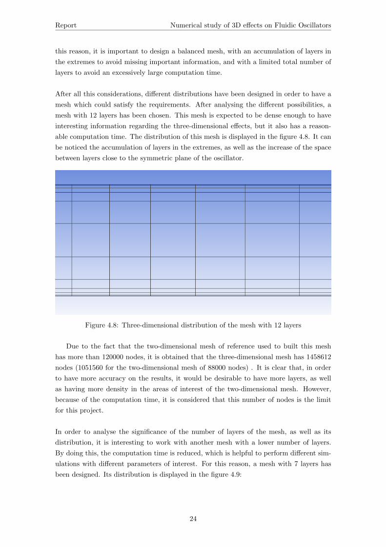
After all this considerations, different distributions have been designed in order to have a
mesh which could satisfy the requirements. After analysing the different possibilities, a
mesh with 12 layers has been chosen. This mesh is expected to be dense enough to have
interesting information regarding the three-dimensional effects, but it also has a reason-
able computation time. The distribution of this mesh is displayed in the figure 4.8. It can
be noticed the accumulation of layers in the extremes, as well as the increase of the space
between layers close to the symmetric plane of the oscillator.
Figure 4.8: Three-dimensional distribution of the mesh with 12 layers
Due to the fact that the two-dimensional mesh of reference used to built this mesh
has more than 120000 nodes, it is obtained that the three-dimensional mesh has 1458612
nodes (1051560 for the two-dimensional mesh of 88000 nodes) . It is clear that, in order
to have more accuracy on the results, it would be desirable to have more layers, as well
as having more density in the areas of interest of the two-dimensional mesh. However,
because of the computation time, it is considered that this number of nodes is the limit
for this project.
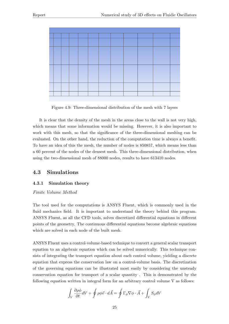
In order to analyse the significance of the number of layers of the mesh, as well as its
distribution, it is interesting to work with another mesh with a lower number of layers.
By doing this, the computation time is reduced, which is helpful to perform different sim-
ulations with different parameters of interest. For this reason, a mesh with 7 layers has
been designed. Its distribution is displayed in the figure 4.9:
24
Page 32
Report Numerical study of 3D effects on Fluidic Oscillators
Figure 4.9: Three-dimensional distribution of the mesh with 7 layers
It is clear that the density of the mesh in the areas close to the wall is not very high,
which means that some information would be missing. However, it is also important to
work with this mesh, so that the significance of the three-dimensional meshing can be
evaluated. On the other hand, the reduction of the computation time is always a benefit.
To have an idea of this the mesh, the number of nodes is 850857, which means less than
a 60 percent of the nodes of the densest mesh. This three-dimensional distribution, when
using the two-dimensional mesh of 88000 nodes, results to have 613410 nodes.
4.3 Simulations
4.3.1 Simulation theory
Finite Volume Method
The tool used for the computations is ANSYS Fluent, which is commonly used in the
fluid mechanics field. It is important to understand the theory behind this program.
ANSYS Fluent, as all the CFD tools, solves discretized differential equations in different
points of the geometry. The continuous differential equations become algebraic equations
which are solved in each node of the built mesh.
ANSYS Fluent uses a control-volume-based technique to convert a general scalar transport
equation to an algebraic equation which can be solved numerically. This technique con-
sists of integrating the transport equation about each control volume, yielding a discrete
equation that express the conservation law on a control-volume basis. The discretization
of the governing equations can be illustrated most easily by considering the unsteady
conservation equation for transport of a scalar quantity . This is demonstrated by the
following equation written in integral form for an arbitrary control volume V as follows:∫V
∂ρφ
∂tdV +
∮ρφ~v · d ~A =
∮Γφ∇φ · ~A+
∫VSφdV
25
Page 33
Report Numerical study of 3D effects on Fluidic Oscillators
where ρ is the density, ~v is the velocity vector, ~A is the surface area vector, Γφ is the
diffusion coefficient for φ and Sφ is a source of φ per unit volume. This equation is applied
to each control volume or cell in the computational domain. The discretization of this
equation can be written as follows:
∂ρφ
∂tV + ΣNfaces
f ρf~vfφf ~Af = ΣNfacesf Γφ∇φf ~Af + SφV
where Nfaces is the number of faces enclosing the cell, φf is the value of φ convected
through the face f, ρf~vf ~Af is the mass flux through the face, ~Af is the area of face f and V
is the cell volume. All the equations solved by ANSYS Fluent take this general form (for
example, the momentum equation in the component x results from imposing φ = u). This
equation, in general, is non linear with respect to the unknown variables (the variable φ
at the cell center and the values in the surrounding neighbour cells), but a linearized form
can be written as:
aPφ = Σnbanbφnb + b
where nb means neighbour cells, and aP and anb are the linearised coefficients for φ and
φnb. For each cell it is obtained an equation with this form, which results in a set of
algebraic equations with a sparse coefficient matrix, solved by the program.
For all flows, ANSYS Fluent solves conservation equations for mass and momentum. Apart
from these equations, for flows involving heat transfer or compressibility, it is also solved
the energy conservation equation, and when the flow is turbulent additional transport
equations are also solved.
The continuity equation, or equation for conservation of mass, can be written as follows:
∂ρ
∂t+∇ · (ρ~v) = 0
This equation is the general form of the mass conservation equation, so it is valid for
compressible and incompressible flow.
Regarding the momentum conservation equation,the x-component can be written as fol-
lows::
ρDu
Dt=∂(−p+ τxx)
∂x+∂τyx∂y
+∂τzx∂x
+ SMx
where p is the pressure (normal stress); τxx, τyx and τzx are components of the viscous
stress, u is the velocity in the x direction and SMx is a source of x-momentum per unit
volume per unit time, which considers the overall effect of the body forces. In the other
two components the equation is analogue.
As it has been mentioned before, it is also solved the energy equation:
ρDe
Dt= ρq +
∂
∂x(k∂T
∂x) +
∂
∂y(k∂T
∂y) +
∂
∂z(k∂T
∂z) − p(
∂u
∂x+∂v
∂y+∂w
∂z) + λ(
∂u
∂x+∂v
∂y+
26
Page 34
Report Numerical study of 3D effects on Fluidic Oscillators
∂w
∂z)2 + µ[2(
∂u
∂x)2 + 2(
∂v
∂y)2 + 2(
∂w
∂z)2 + (
∂u
∂y+∂v
∂x)2 + (
∂u
∂z+∂w
∂x)2 + (
∂v
∂z+∂w
∂y)2]
where u,v and w are the three components of the velocity, e is the internal energy per
unit mass, q is the rate of volumetric heat addition per unit mass, k is the thermal con-
ductivity, T is the temperature and p is the pressure.
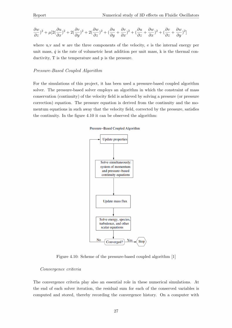
Pressure-Based Coupled Algorithm
For the simulations of this project, it has been used a pressure-based coupled algorithm
solver. The pressure-based solver employs an algorithm in which the constraint of mass
conservation (continuity) of the velocity field is achieved by solving a pressure (or pressure
correction) equation. The pressure equation is derived from the continuity and the mo-
mentum equations in such away that the velocity field, corrected by the pressure, satisfies
the continuity. In the figure 4.10 it can be observed the algorithm:
Figure 4.10: Scheme of the pressure-based coupled algorithm [1]
Convergence criteria
The convergence criteria play also an essential role in these numerical simulations. At
the end of each solver iteration, the residual sum for each of the conserved variables is
computed and stored, thereby recording the convergence history. On a computer with
27
Page 35
Report Numerical study of 3D effects on Fluidic Oscillators
infinite precision, these residuals will go to zero as the solution converges. On an actual
computer, the residuals decay to some small value (“round-off”) and then stop changing
(“level out”). The computations performed in this project are double-precision compu-
tations, which means that the residuals can drop as many as twelve orders of magnitude
before hitting round-off.
As it has been mentioned previously, the conservation equation for a general variable
φ at a cell P can be written as follows:
aPφ = Σnbanbφnb + b
where aP is the center coefficient, anb are the influence coefficients for the neighbouring
cells and b is the contribution of the constant part of the source term Sc in S = Sc +SPφ
and of the boundary conditions. In the previous equation:
aP = Σnbanb − SP
The residual Rφ computed by the pressure-based solver of ANSYS is the imbalance in
the conservation equation summed over all the computational cells P. This is refered to
an ”unscaled” residual. However, it is difficult to judge convergence by examining this
non-scaled residuals. For this reason, ANSYS Fluent scales the residual using two kinds
of scaling factors, representative of the flow rate φ through the domain: the global scaling
and the local scaling. The ”global scalled” is defined as follows:
Rφ =ΣcellsP |Σnbanb + b− apφp|
ΣcellsP |apφp|
The ”locally scaled” residual is defined as follows:
Rφ =
√(Σn
cells(1n)(
Σnbanb+b−apφpaP
)2
(φmax − φmin)domain
For the simulations launched in this project, the default ANSYS Fluent convergence crite-
rion have been used. This criterion requires that the ”globally scaled” residuals decrease to
a 10−3 for all equations except the P-1 (for radiation problems) and the energy equations.
Regarding the ”locally scaled” residuals, it is required a decrease of 10−5 Turbulence
is a three-dimensional unsteady random motion observed in fluids at moderate to high
Reynolds numbers. Technical flows are typically based on fluids of low viscosity, which
means that almost all the technical flows are turbulent.
Turbulence
Turbulence is described by the Navier-Stokes equations, but in most situations it is not
possible to solve the problem by Direct Numerical Simulation (DNS) due to the fact that
CPU requirements would by far exceed the available computing power. For this reason,
28
Page 36
Report Numerical study of 3D effects on Fluidic Oscillators
averaging procedures are applied to the Navier-Stokes equations, and the most widely
applied averaging procedure is Reynolds averaging, resulting in the Reynolds-Averaged
Navier-Stokes (RANS) equations. With this process, the turbulent structures are elimi-
nated from the flow, and a smooth variation of the averaged velocity and pressure fields
can be obtained.
It is important to remark that the averaging process adds additional unknown terms
into the transport equations (Reynolds Stresses and Fluxes) that need to be provided by
suitable turbulence models (turbulence closures). The most used models are those which
provide two new equations to the system, such as k-ε and k-ω. The model k-ε links the
kinetic energy k and the dissipation velocity ε with partial derivation. The dissipation ve-
locity ε represents the energy flux which is transmitted from the big swirls to the smaller
swirls described in the classical theory of turbulence of Kolmogorov [13]. The model k-ω
links the kinetic energy k with the specific dissipation ω. In both cases, the two equations
give the parameters to compute the dynamical viscosity, necessary to solve the discretized
Navier-Stokes equations. Both models assume a turbulent flux, even in the boundary layer.
The quality of the simulation and the accuracy of the results are directly related with
the chosen turbulence model. As it has been mentioned previously in this report, the
model selected by Bobusch [3] has been k-ε Shear-Stress Transport (SST). This model is
based on k-ε model, but ensures the exact prediction of the flux separation by treating
the solid walls as rough walls. However, most of the simulations of Ruiz [22] were done
with the model Transition SST, so this is the model selected for this project too, in order
to compare the two-dimensional and three-dimensional results with the same parameters
of simulation. This model does not assume turbulent flux in the boundary layer like the
k-ε: it solves the boundary layer from the laminar zone to the turbulent zone. As it is
explained in Ruiz’s thesis, the difference between the results of the simulations using both
models is acceptable.
Solution Methods
For the pressure-velocity coupling, the algorithm used is SIMPLE. The SIMPLE algorithm
uses a relationship between velocity and pressure corrections to enforce mass conservation
and to obtain the pressure field.
Regarding the spatial discretization, it is important to mention that ANSYS Fluent stores
discrete values of the scalar φ at the cell centres. However, the face values φf are required
for convection terms and must be interpolated from the cell center values. The way to do
this is by using an upwind scheme, which means that the face value φf is derived from
quantities in the cell upstream (or upwind) relative to the direction of the normal velocity
vn. In this simulations, the scheme chosen for momentum, turbulent kinetic energy, spe-
cific dissipation rate, intermittency and momentum thickness re has been a First-Order
29
Page 37
Report Numerical study of 3D effects on Fluidic Oscillators
Upwind Scheme, which means that the quantities at the cell faces are determined by as-
suming that the cell-center values of any field variable represent a cell-average value, which
can be considered as constant in the whole cell. With this method, the face quantities
are identical to the cell quantities, which means that the face value φf is set equal to the
cell-center value of φ in the upstream cell.
For the pressure, the discretization is Standard. This method interpolates the pressure
values at the faces using momentum equation coefficients. This procedure has good results
as long as the pressure variation between the cells is smooth, as it is supposed to be in
this case.
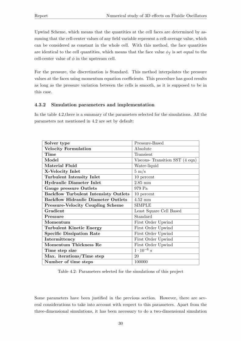
4.3.2 Simulation parameters and implementation
In the table 4.2,there is a summary of the parameters selected for the simulations. All the
parameters not mentioned in 4.2 are set by default:
Solver type Pressure-Based
Velocity Formulation Absolute
Time Transient
Model Viscous- Transition SST (4 eqn)
Material Fluid Water-liquid
X-Velocity Inlet 5 m/s
Turbulent Intensity Inlet 10 percent
Hydraulic Diameter Inlet 2.85 mm
Gauge pressure Outlets 979 Pa
Backflow Turbulent Intensisty Outlets 10 percent
Backflow Hidraulic Diameter Outlets 4.52 mm
Pressure-Velocity Coupling Scheme SIMPLE
Gradient Least Square Cell Based
Pressure Standard
Momentum First Order Upwind
Turbulent Kinetic Energy First Order Upwind
Specific Dissipation Rate First Order Upwind
Intermittency First Order Upwind
Momentum Thickness Re First Order Upwind
Time step size 1 · 10−6 s
Max. iterations/Time step 20
Number of time steps 100000
Table 4.2: Parameters selected for the simulations of this project
Some parameters have been justified in the previous section. However, there are sev-
eral considerations to take into account with respect to this parameters. Apart from the
three-dimensional simulations, it has been necessary to do a two-dimensional simulation
30
Page 38
Report Numerical study of 3D effects on Fluidic Oscillators
with the less dense mesh of 88000 nodes, as it has been mentioned previously. In this case,
all the parameters selected are the explained in the table, but adding the fact that the 2D
Space of the solver is Planar.
First of all, the simulations should not be launched directly. It is advisable to have an
initial solution to accelerate the convergence of the transient solution, and that is even
more important for the three-dimensional simulations of this project, which have a larger
computation time. In order to have an initial solution to start the transient simulations, a
previous turbulent steady simulation has been launched for each case (apart from chang-
ing the Time to ”Transient”, the other parameters do not change). Alternatively, it has
been done an three-dimensional interpolation from the two-dimensional results obtained
by Ruiz, in order to have another initial solution. However, this alternative has been
discarded, due to the fact that it is needed more time for the solution to converge in
comparison with initializing from the steady turbulent solution.
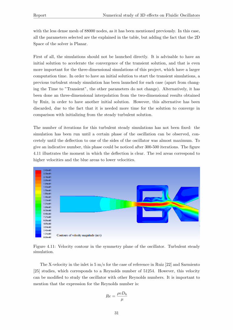
The number of iterations for this turbulent steady simulations has not been fixed: the
simulation has been run until a certain phase of the oscillation can be observed, con-
cretely until the deflection to one of the sides of the oscillator was almost maximum. To
give an indicative number, this phase could be noticed after 300-500 iterations. The figure
4.11 illustrates the moment in which the deflection is clear. The red areas correspond to
higher velocities and the blue areas to lower velocities.
Figure 4.11: Velocity contour in the symmetry plane of the oscillator. Turbulent steadysimulation.
The X-velocity in the inlet is 5 m/s for the case of reference in Ruiz [22] and Sarmiento
[25] studies, which corresponds to a Reynolds number of 51254. However, this velocity
can be modified to study the oscillator with other Reynolds numbers. It is important to
mention that the expression for the Reynolds number is:
Re =ρvDh
µ
31
Page 39
Report Numerical study of 3D effects on Fluidic Oscillators
where v in this case is the velocity in the power nozzle, ρ is the density of the water, Dh
is the hydraulic diameter of the power nozzle and µ is the dynamic viscosity of the water.
This criteria to determine the Reynolds number was established in Bobusch’s experimental
study [4].
The Turbulent Intensity is a parameter used to quantify the perturbation of the fluid.
It is defined as the root of the velocity fluctuations divided by the average velocity.For
this simulations, this parameter is a 10 percent.
The hydraulic diameter (Dh) is a parameter which is used to study the jet in a non
circular duct as if it was circular. It can be computed by applying the expression:
Dh =4A
P
where A is the section of the duct and P is the perimeter. From the geometry of the
oscillator of study, it is found that the hydraulic diameter is 2.85 mm for the inlet and
4.52 mm for the outlets.
The size of the time step, as well as the number of time steps, are essential parame-
ters in the simulation. Ruiz found that the optimal value of time step was 1 · 10−6, and
that is the value used in the simulations of this project. It is an important value, because
using a bigger time step could suppose missing some information of the simulation and
misunderstanding the results, and using a smaller time step means that it is needed more
time steps to obtain the same time in the simulations.
Regarding the number of time steps, it is not always 100000. With an inlet velocity
of 5 m/s (Reynolds number 51254), the frequency of oscillation obtained by Ruiz and
Sarmiento was 46.843 Hz. With this frequency, the period is 0.021 s. With the size of
time step of this simulations, using 100000 means covering 0.1 s, which theoretically is
enough to observe more than four cycles. However, it has to be considered that the initial
time steps correspond to not converged solution, which means that it is needed a certain
margin of time until the solution is the desired. For this reason, it is important to take
this into account when setting the number of time steps. Apart from this fact, differ-
ent inlet velocities mean different frequencies of oscillation, so it can be needed more or
less time to obtain, at least, the results corresponding to two complete cycles without noise.
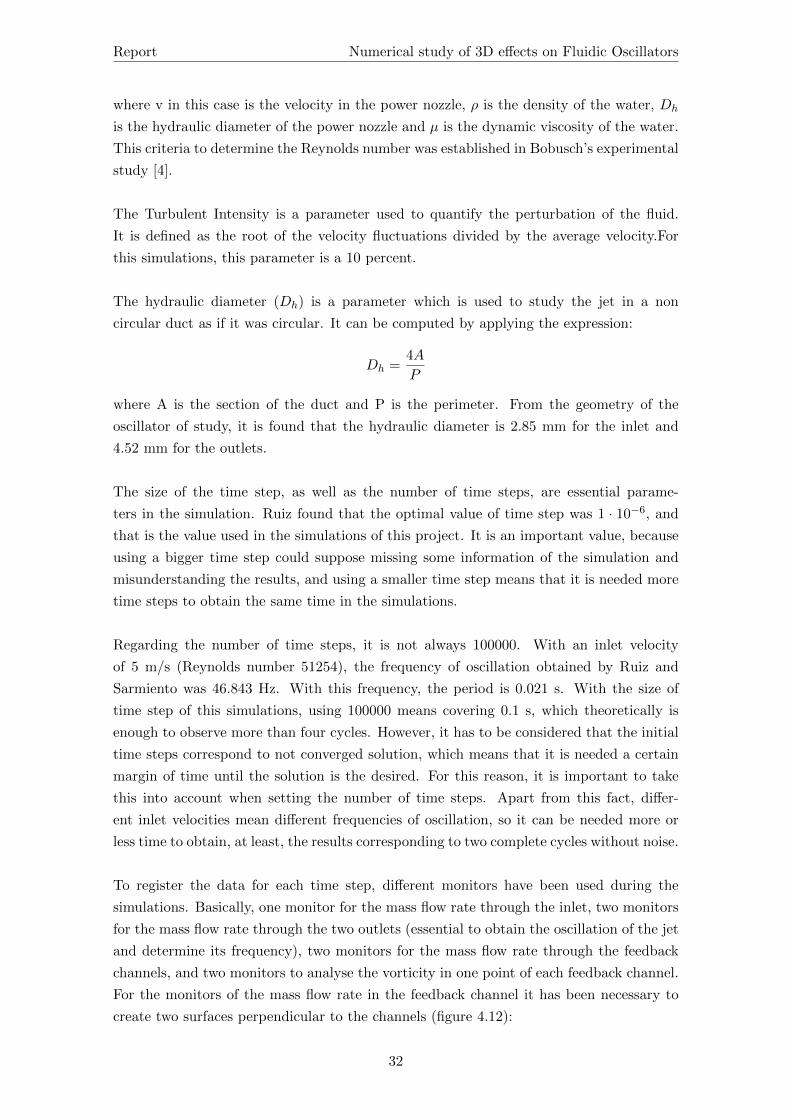
To register the data for each time step, different monitors have been used during the
simulations. Basically, one monitor for the mass flow rate through the inlet, two monitors
for the mass flow rate through the two outlets (essential to obtain the oscillation of the jet
and determine its frequency), two monitors for the mass flow rate through the feedback
channels, and two monitors to analyse the vorticity in one point of each feedback channel.
For the monitors of the mass flow rate in the feedback channel it has been necessary to
create two surfaces perpendicular to the channels (figure 4.12):
32
Page 40
Report Numerical study of 3D effects on Fluidic Oscillators
Figure 4.12: Surfaces and points used for monitoring the results in the feedback channels
Taking into account that the computation time is large, it has also been useful to
register all the data every certain number of time steps, to avoid losing the progress in
case the simulation stops unexpectedly because of an error. It has been mentioned several
times that the computation time needed for the three-dimensional simulations is high, due
to the number of nodes which the meshes have. With a personal computer it is not possible
to do such simulations. For this reason, the cluster of the ETSEIAT has been used, in
order to decrease the time needed for the simulations, as well as having the possibility of
launching more than one simulation at the same time.
33
Page 41
Report Numerical study of 3D effects on Fluidic Oscillators
Chapter 5
Results
In this chapter, all the results obtained from the simulations are presented and discussed.
For each simulation, it is showed the mass flow rate in the inlet and both outlets, as well
as the mass flow rate in the feedback channels, obtained by locating a surface monitor in
the middle of the channels. In all the figures presented in this chapter, a negative flow
rate means that the fluid is leaving the control volume (the oscillator), and a positive flow
rate means that the fluid is entering the control volume.
First of all, the results corresponding to the simulations with a Reynolds number of 51254
are displayed. For this Reynolds number, four simulations have been performed, as a result
of the possible combinations for the three-dimensional mesh: the mesh can be based on
a two-dimensional mesh with 120000 or 88000 nodes, and the three-dimensional distribu-
tion can contain 7 or 12 layers (more details of these possibilities are given in the chapter
4). The results obtained from this simulations are compared with the results obtained
with the corresponding two-dimensional simulations. For the three-dimensional meshes
based on the two-dimensional mesh of 120000 nodes, the results are compared with the
two-dimensional simulation performed by Ruiz [22]. However, for the three-dimensional
meshes based on the two-dimensional mesh of 88000 nodes there is no previous simulation,
so it has been necessary to perform a two-dimensional simulation in order to compare the
results. Due to this fact, the results obtained from this two-dimensional simulation are
also displayed in this chapter.
After the simulations with a Reynolds number of 51254, other simulations with differ-
ent Reynolds number (15376 and 30752) have been performed. For reasons of time, only
one mesh has been used for these Reynolds numbers: the one based on the two-dimensional
mesh of 120000 nodes built by Ruiz and with a three-dimensional distribution of 7 layers.
The selection of this mesh is justified later.
Finally, all the results obtained in this project are summarised as well as compared with
the results obtained by Ruiz [22] and Bobusch [3] [4] at the end of this chapter.
34
Page 42
Report Numerical study of 3D effects on Fluidic Oscillators
5.1 Simulations with Reynolds number=51254
5.1.1 3D Mesh based on the 2D mesh of 120000 nodes
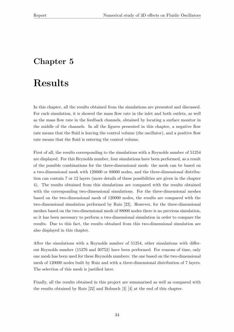
First of all, the results for the mesh based in the two-dimensional mesh of 120000 nodes
of Ruiz and the 3D distribution of 12 layers are presented. The mass flow rate in the inlet
and the outlets are displayed in the figure 5.1:
Figure 5.1: Mass flow rate in the inlet and outlets
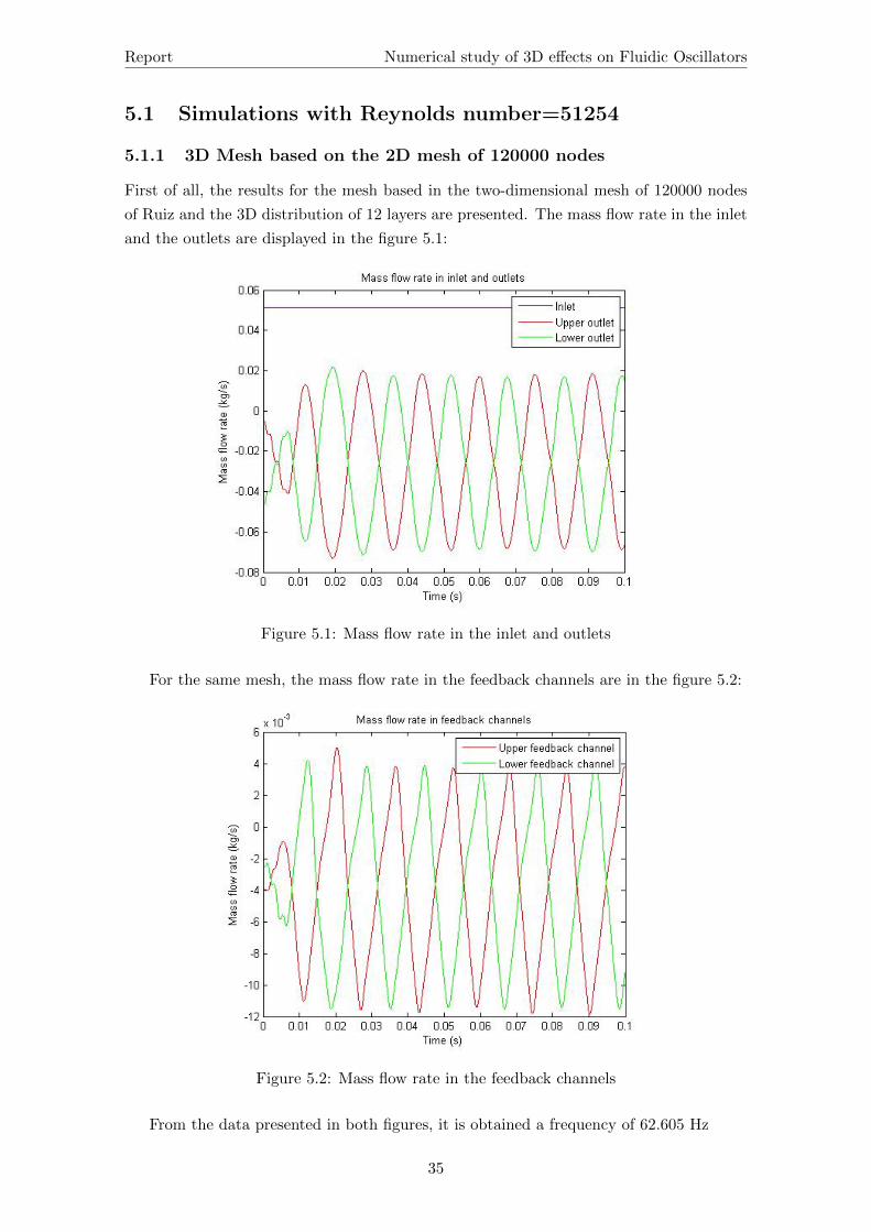
For the same mesh, the mass flow rate in the feedback channels are in the figure 5.2:
Figure 5.2: Mass flow rate in the feedback channels
From the data presented in both figures, it is obtained a frequency of 62.605 Hz
35
Page 43
Report Numerical study of 3D effects on Fluidic Oscillators
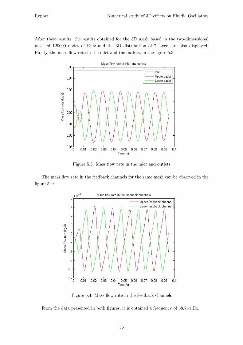
After these results, the results obtained for the 3D mesh based in the two-dimensional
mesh of 120000 nodes of Ruiz and the 3D distribution of 7 layers are also displayed.
Firstly, the mass flow rate in the inlet and the outlets, in the figure 5.3:
Figure 5.3: Mass flow rate in the inlet and outlets
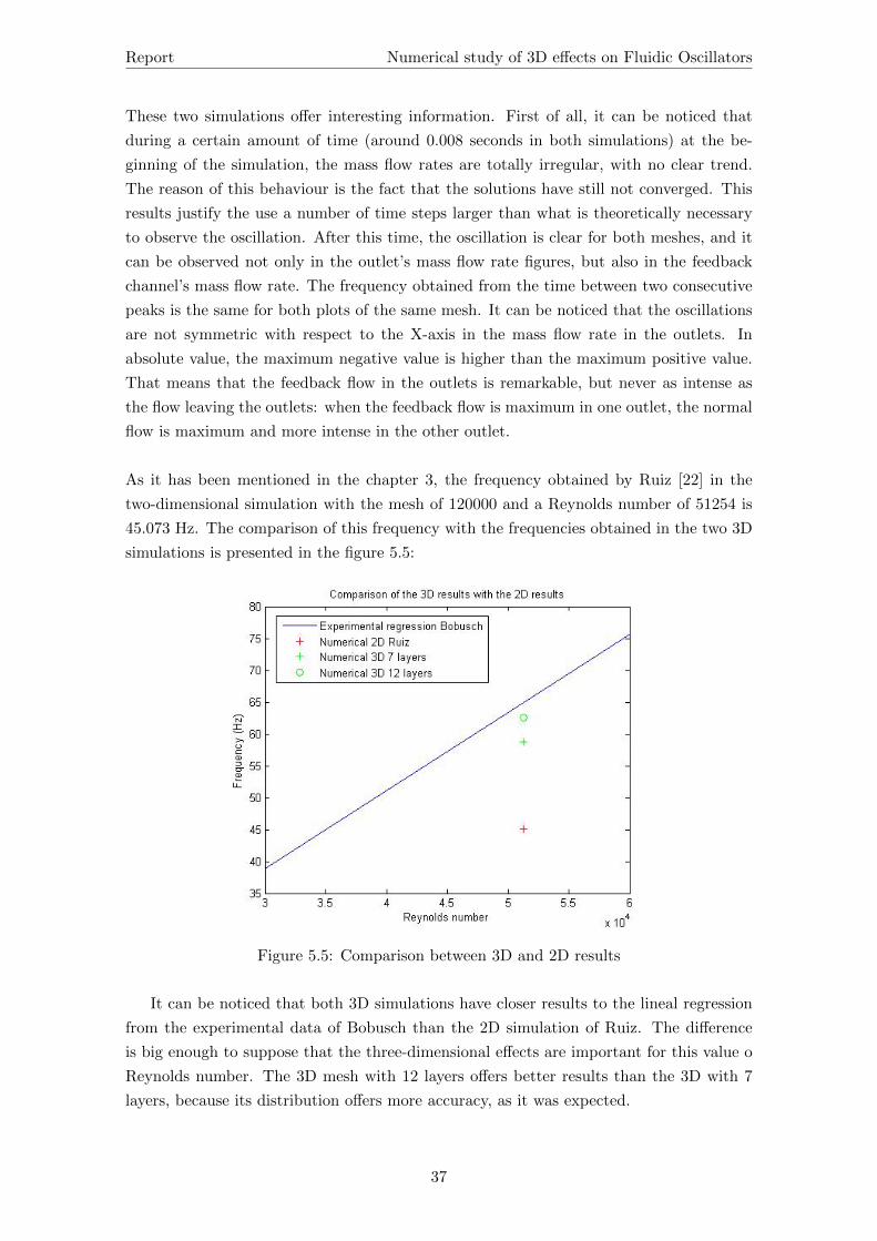
The mass flow rate in the feedback channels for the same mesh can be observed in the
figure 5.4:
Figure 5.4: Mass flow rate in the feedback channels
From the data presented in both figures, it is obtained a frequency of 58.754 Hz.
36
Page 44
Report Numerical study of 3D effects on Fluidic Oscillators
These two simulations offer interesting information. First of all, it can be noticed that
during a certain amount of time (around 0.008 seconds in both simulations) at the be-
ginning of the simulation, the mass flow rates are totally irregular, with no clear trend.
The reason of this behaviour is the fact that the solutions have still not converged. This
results justify the use a number of time steps larger than what is theoretically necessary
to observe the oscillation. After this time, the oscillation is clear for both meshes, and it
can be observed not only in the outlet’s mass flow rate figures, but also in the feedback
channel’s mass flow rate. The frequency obtained from the time between two consecutive
peaks is the same for both plots of the same mesh. It can be noticed that the oscillations
are not symmetric with respect to the X-axis in the mass flow rate in the outlets. In
absolute value, the maximum negative value is higher than the maximum positive value.
That means that the feedback flow in the outlets is remarkable, but never as intense as
the flow leaving the outlets: when the feedback flow is maximum in one outlet, the normal
flow is maximum and more intense in the other outlet.
As it has been mentioned in the chapter 3, the frequency obtained by Ruiz [22] in the
two-dimensional simulation with the mesh of 120000 and a Reynolds number of 51254 is
45.073 Hz. The comparison of this frequency with the frequencies obtained in the two 3D
simulations is presented in the figure 5.5:
Figure 5.5: Comparison between 3D and 2D results
It can be noticed that both 3D simulations have closer results to the lineal regression
from the experimental data of Bobusch than the 2D simulation of Ruiz. The difference
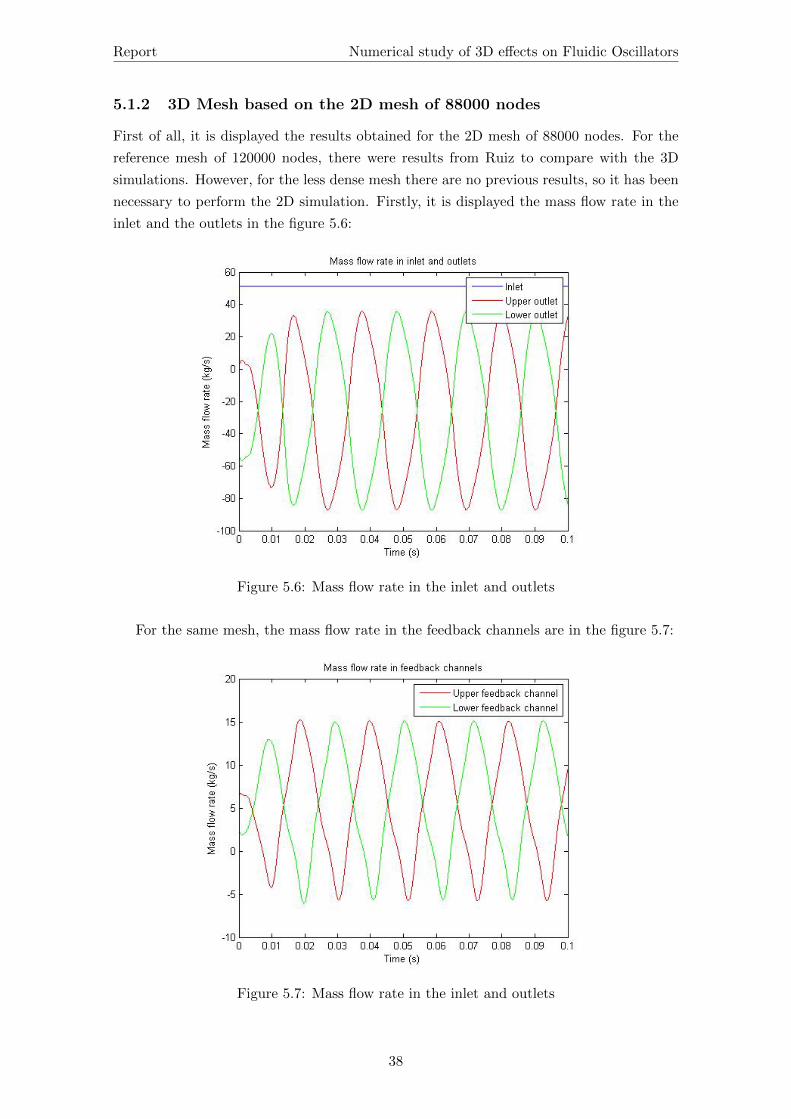
is big enough to suppose that the three-dimensional effects are important for this value o
Reynolds number. The 3D mesh with 12 layers offers better results than the 3D with 7
layers, because its distribution offers more accuracy, as it was expected.
37
Page 45
Report Numerical study of 3D effects on Fluidic Oscillators
5.1.2 3D Mesh based on the 2D mesh of 88000 nodes
First of all, it is displayed the results obtained for the 2D mesh of 88000 nodes. For the
reference mesh of 120000 nodes, there were results from Ruiz to compare with the 3D
simulations. However, for the less dense mesh there are no previous results, so it has been
necessary to perform the 2D simulation. Firstly, it is displayed the mass flow rate in the
inlet and the outlets in the figure 5.6:
Figure 5.6: Mass flow rate in the inlet and outlets
For the same mesh, the mass flow rate in the feedback channels are in the figure 5.7:
Figure 5.7: Mass flow rate in the inlet and outlets
38
Page 46
Report Numerical study of 3D effects on Fluidic Oscillators
From the data presented in both figures, it is obtained a frequency of 47.411 Hz. After
this previous analysis, the results for the mesh based in the two-dimensional mesh of 88000
nodes and the 3D distribution of 12 layers are presented. The mass flow rate in the inlet
and the outlets are displayed in the figure 5.8:
Figure 5.8: Mass flow rate in the inlet and outlets
It is also displayed the mass flow rate in the feedback channels for the same mesh, in
the figure 5.9:
Figure 5.9: Mass flow rate in the feedback channels
From both graphics and their data, it is observed a frequency of 62.305 Hz.
39
Page 47
Report Numerical study of 3D effects on Fluidic Oscillators
After the 3D mesh with 12 layers, the results obtained for the 3D mesh based in the
two-dimensional mesh of 88000 nodes of Ruiz and the 3D distribution of 7 layers are
displayed. Firstly, the mass flow rate in the inlet and the outlets, in the figure 5.10:
Figure 5.10: Mass flow rate in the inlet and outlets
It is also displayed the mass flow rate in the feedback channels for the same mesh, in
the figure 5.11:
Figure 5.11: Mass flow rate in the feedback channels
From both graphics and their data, it is observed a frequency of 57.654 Hz.
40
Page 48
Report Numerical study of 3D effects on Fluidic Oscillators
It is important to analyse the results of the two-dimensional simulation, which will be
the reference results to do the comparison with the three-dimensional simulations. The
behaviour of the oscillator in the two-dimensional simulation is as it was expected. The
time necessary for having a converged solution is not very large (about 0.005 seconds), and
after completing one oscillation cycle, the results are stable. The frequency of oscillation
is 47.411 Hz for this two-dimensional simulation, which is close to the two-dimensional
simulation based on the mesh of 120000 performed by Ruiz (45.073 Hz).
Regarding the three-dimensional simulations, the period of instability of the results is
also around 0.005 seconds. It is observed, as it happened in the previous simulations,
that the maximum negative value of mass flow rate is bigger in absolute value than the
maximum positive value. As it has been mentioned previously, the feedback flow in the
outlets is never as intense as the normal flow.
A comparison between the two-dimensional simulation and the three -dimensional sim-
ulations is illustrated in the figure 5.12:
Figure 5.12: Comparison between 3D and 2D results
In this figure it can be noticed that the three-dimensional simulations have closer
frequencies to the linear regression of the experimental results of Bobusch. The results
show, as it happened in the previous simulations, that the three-dimensional effects are
important for high Reynolds number. The simulation with the 3D mesh with a distribution
of 12 layers has closer results to the experimental data, due to the fact that the there is
more accumulation of layers in the areas close to the walls than in the 3D mesh with 7
layers.
41
Page 49
Report Numerical study of 3D effects on Fluidic Oscillators
5.2 Simulation with Reynolds number=30752
The results obtained for a Reynolds number of 30752 with the mesh based on a two-
dimensional mesh of 120000 and 7 layers are displayed in the figure 5.13:
Figure 5.13: Mass flow rate in the inlet and outlets
It is also displayed the mass flow rate in the feedback channels for the same Reynolds
number (figure 5.14):
Figure 5.14: Mass flow rate in the feedback channels
From both graphics and their data, it is observed a frequency of 37.322 Hz.
42
Page 50
Report Numerical study of 3D effects on Fluidic Oscillators
It is interesting to analyse the results obtained for the Reynolds number of 30752. The
comparison between the frequency obtained in this three-dimensional analysis and the
two-dimensional analysis of Ruiz is illustrated in the figure 5.15:
Figure 5.15: Comparison between 3D and 2D results
Considering the experimental results obtained by Bobusch as the reference data, it
is clear that the three-dimensional results are closer to the reference data than the two-
dimensional results of Ruiz. This difference is around 7 Hz, which is smaller than the
difference observed for the Reynolds number of 51254 (more than 13 Hz). However, this
difference is clearly bigger than the difference observed in Bobusch analysis (around 2Hz),
and it can not be ignored.
The reduction of the difference between the two-dimensional and the three-dimensional
analysis could mean that the importance of the three-dimensional effects is lower with
lower Reynolds numbers (less turbulence). It is necessary, however, to confirm this trend
with the results obtained for lower Reynolds number. On the other hand, this discrepan-
cies are more important than the discrepancies noticed by Bobusch, who worked with a
narrower range of Reynolds number. For this reason, the performance of three-dimensional
analysis has more sense than in Bobusch’s studies.
It is important to take into account that by using the mesh of 7 layers it is obtained
an approximate result for the frequency, but it is not an exact result. Further analysis
with better meshes should be performed in order to increase the accuracy and confirm the
results.
43
Page 51
Report Numerical study of 3D effects on Fluidic Oscillators
5.3 Simulation with Reynolds number of 15376
The results obtained for a Reynolds number of 15376 with the mesh based on a two-
dimensional mesh of 120000 and 7 layers are displayed in the figure 5.16:
Figure 5.16: Mass flow rate in the inlet and outlets
It is also displayed the mass flow rate in the feedback channels for the same Reynolds
number (figure 5.17):
Figure 5.17: Mass flow rate in the feedback channels
From both graphics and their data, it is observed a frequency of 21.759 Hz.
44
Page 52
Report Numerical study of 3D effects on Fluidic Oscillators
It is interesting to analyse the results obtained for the Reynolds number of 15376. The
comparison between the frequency obtained in this three-dimensional analysis and the
two-dimensional analysis of Ruiz is illustrated in the figure 5.18:
Figure 5.18: Comparison between 3D and 2D results
As it has been considered previously, the experimental results obtained by Bobusch
are the reference data. Again, the three-dimensional results are closer to the reference
data than the two-dimensional results of Ruiz. However, this difference is smaller than in
the simulations with larger Reynolds numbers. This difference is around 6 Hz, which is
smaller than the difference observed for the Reynolds number of 30752 (around 7 Hz).
This Reynolds number is included in the range of Reynolds studied by Bobusch. It is
clear, however, that the differences between 2D and 3D are bigger than the results of
Bobusch (2 Hz). The accuracy of the results could be not high enough, which could jus-
tify the discrepancies. It is important to remember that the mesh used for this analysis is
not the one with the highest accuracy, which means that the result is an approximation
but never an exact result. The use of meshes with a better design is advisable.
On the other hand ,the reduction of the difference between the two-dimensional and the
three-dimensional analysis is not as clear as in the previous simulation. However, the
trend is still the same, which is a signal that, as it has been mentioned before, the three-
dimensional effects are weakened with lower Reynolds numbers. It could be interesting to
confirm this trend with the results obtained for other Reynolds number.
45
Page 53
Report Numerical study of 3D effects on Fluidic Oscillators
5.4 Summary of results and comparison with the previous
studies
One important parameter in the simulations of this project has been the computation
time. In the table 5.1 it is shown, for each mesh, the necessary time to obtain the solution
with 100000 time steps:
Mesh Time
3D Mesh (2D 120000 nodes + 12 layers) 23 days 15 hours
3D Mesh (2D 120000 nodes + 7 layers) 12 days 9 hours
3D Mesh (2D 88000 nodes + 12 layers) 17 days 10 hours
3D Mesh (2D 88000 nodes + 7 layers) 10 days 2 hours
Table 5.1: Computation time for the different simulations
The analysis of the necessary time for each simulation has been essential in order to se-
lect the mesh to perform simulations with other Reynolds numbers. The three-dimensional
mesh based on the two-dimensional mesh of 120000 nodes and a distributions with 7 lay-
ers has been selected for this simulations. The interest of comparing the results obtained
in a two-dimensional analysis, and the fact that Ruiz [22] obtained results for different
Reynolds with the mesh of 120000 nodes makes interesting to select the first or the second
mesh in the table 5.1, so that only the three-dimensional effects can modify the results.
However, the computation time of the first mesh is too high for the available time, there-
fore the second option has been chosen.
To have a general perspective of the results obtained in the simulations, the different
frequencies are summarised in the table 5.2:
Re=51254 Re=30752 Re=15376
3D Mesh (2D 120000 nodes + 12 layers) 62.605 Hz - -
3D Mesh (2D 120000 nodes + 7 layers) 58.754 Hz 37.322 21.759
3D Mesh (2D 86000 nodes + 12 layers) 62.305 Hz - -
3D Mesh (2D 86000 nodes + 7 layers) 57.654 Hz - -
2D Mesh 86000 nodes 47.411 Hz - -
Table 5.2: Summary of the results obtained from the simulations
In the figure 5.19 it can be observed the comparison between the experimental and
numerical data of Bobusch, the numerical data of Ruiz and the three-dimensional analysis
of this project:
46
Page 54
Report Numerical study of 3D effects on Fluidic Oscillators
Figure 5.19: Frequency as a function of the Reynolds number
The results obtained with the different simulations offer interesting information with
respect to the three-dimensional effects in the fluidic oscillator. Bobusch [3] found that
the computational cost derivative from performing a three-dimensional analysis was too
high to be compensated by the increase of the accuracy of the results. However, his stud-
ies were limited by a relatively narrow range of Reynolds numbers (8711-18034). Ruiz
[22] performed simulations with a wider range of Reynolds number (8711-51253), and he
found some discrepancies with the oscillation frequency values at high Reynolds number.
The linear trend observed by Bobusch in his experimental and numerical results for the
frequency as a function of the Reynolds number (or velocity in the inlet) was becoming
less clear for these high Reynolds values, as it can be noticed in the figure 5.19.
The results of this project, for a high Reynolds number (51254), are closer to the lin-
ear trend than the results obtained by Ruiz. Due to this fact, it can be supposed that
the three-dimensional effects have more significance in a turbulent regime, with a higher
Reynolds number. Taking this into account, it seems that developing a three-dimensional
analysis, for this higher velocities, is interesting and advisable to do, in order to avoid los-
ing important information. The discrepancies with the two-dimensional analysis of Ruiz
big enough to consider them. It is possible that the density and the distribution of the
two-dimensional mesh has also an impact on the results, and this could partially justify the
discrepancies, because the mesh used by Bobusch has more than 160000 nodes, while the
mesh from Ruiz has only 120000. However, it has been observed that the differences be-
tween the different two-dimensional mesh distributions are not so high to explain a gap of
more than 15 Hz. Furthermore, the results obtained for lower Reynolds number continue
are also closer to the experimental data obtained by Bobusch. However, the difference
between the 2D and the 3D analysis are lower for these Reynolds number, which seems
47
Page 55
Report Numerical study of 3D effects on Fluidic Oscillators
to confirm that the three-dimensional effects are important in turbulent flows (higher
Reynolds number), and they lose importance when the Reynolds number is lower.
Another conclusion which can be extracted from the results is that the influence of the
three-dimensional distribution is important, but the differences are not excessively high.
It has been found a difference of 2-3 Hz between the three-dimensional meshes with 7
layers or 12 layers (table 5.2). Due to this fact, meshes with a lower number of nodes can
be used to perform simulations with different Reynolds numbers to have an approximation
of the frequencies at these regimes. With denser meshes, the computation time needed to
obtain results would have been too high. However, with meshes with a lower number of
nodes, this simulations have been possible.
48
Page 56
Report Numerical study of 3D effects on Fluidic Oscillators
Chapter 6
Budget
This chapter has the aim of evaluating the economical expenses which have been necessary
to develop the project. There are different type of expenses to take into account. All of
them are listed in the table 6.1.
Labour Costs
Task e/h Time (h) Total Cost (e)
CFD and ANSYS formation 12 25 300
Cases preparation 12 120 1200
Computations 12 50 600
Post processing 12 30 360
Report 12 80 960
Total labour cost 12 305 3660
Computational Resources
Task e/h Time (h) Total Cost (e)
ANSYS ICEM 0.811 145 117.6
ANSYS FLUENT 2.343 1500 3514.5
Matlab Licence 0.228 30 6.84
Total computational Resources 2.172 1675 3638.94
Additional expenses
Task e/h Time (h) Total Cost (e)
ANSYS Fluent Course 7.14 7 50
Trip Berlin-Barcelona - - 120
Total additional expenses - - 170
Table 6.1: Summary of the expenses derived from this project
As a conclusion, the total cost of the project is 7468.94 e.
49
Page 57
Report Numerical study of 3D effects on Fluidic Oscillators
Chapter 7
Environmental analysis
As it has been mentioned in the previous chapters, the study of fluidic oscillators is very
interesting because of different reasons. One of them is the efficiency of this devices
comparing them with others with the same applications, which is also positive for the
environment.
One of the possible applications of fluidic oscillators is working as a high lift device.
All the high lift devices permit having a lower velocity keeping the same flight altitude.
That means a reduction of the fuel consume, which means a reduction of the emissions to
the atmosphere, as well as a decrease of the resources spent during the flight.
Focusing on the fluidic oscillator itself, it can apply momentum to the boundary layer
and retard the stall, and the difference with other devices with the same function is that it
is a passive device, which means that no electrical power is needed. Due to this fact, they
are clearly more efficient than the alternatives, and there are no emissions to the atmo-
sphere. It is also remarkable that the lack of mobile parts and the simplicity of the design
reduces the costs and the risk of failure. The production of this devices and its mainte-
nance require less resources, and it can also suppose a reduction of the pollution emissions
derived from this processes. Apart from this, these devices are lighter than other high
lift devices, and this reduction of weight implies less lift needed during the flight, which
results in a reduction of the fuel spent, as well as the emissions to the atmosphere.
Fluidic oscillators are also used as calibration tools. Comparing the with other calibration
tools (shock tube facilities, periodic shock wave generators, etc.), fluidic oscillators have
less costs and they are easier to produce, which means that less resources are spent.
Another remarkable application of fluidic oscillatirs is the jet mixing. Probably, this
application is the one with the clearest influence on the environment. Fluidic oscillators
can be used in a combustion chamber to improve the mixing of the different components,
which means a more efficient combustion and a reduction of the production of polluting
gas. This improvement of the combustion efficiency can be noticed in the figures 7.1 and
7.2:
50
Page 58
Report Numerical study of 3D effects on Fluidic Oscillators
Figure 7.1: Concentrations of CO2 of the fluidic oscillator flame (a) and the plane-jetflame (b) [28]
Figure 7.2: Concentrations of propane of the fluidic oscillator flame (a) and the plane jetflame (b) [28]
Both figures are extracted from a study about controlling the plane-jet flame by a
fluidic oscillator technique [28]. It can be noticed in the figure 7.1 that, in general, the
concentration of CO2 is clearly higher in the fluidic oscillator flame, which means that the
combustion with the fluidic oscillator is more complete. On the other hand, the figure 7.2
shows that the concentration of unburned propane is smaller in the fluidic oscillator flame,
which confirms again the better efficiency of the combustion when this device is used.
51
Page 59
Report Numerical study of 3D effects on Fluidic Oscillators
Chapter 8
Conclusions and
Recommendations
This project has been focused on the study of the three-dimensional effects on fluidic os-
cillators. It has been necessary an approach to the Computational Fluid Dynamics and
the theory behind, as well as a familiarisation with the ANSYS tools, to built and mod-
ify meshes (ANSYS ICEM) and to preprocessi and simulate the different cases (ANSYS
Fluent).
A research about the field of study has been done. It has been found that fluidic os-
cillators are devices with applications not only in the aeronautical field (aerodynamic flow
control), but also in other fields (as a calibration tool, in windshield washers, for mixing
jets of different fluids, etc.). The main advantages of fluidic oscillators are the simplicity of
the design, the absence of mobile parts and the fact that it is a passive device (no electrical
energy is needed). The main disadvantage is that it is necessary to obtain certain entrance
conditions in order to obtain the desired exit conditions. However, there are designs to
avoid this problem, such as piezo-electric fluidic oscillators.
The role of the previous studies with the same fluidic oscillator has been essential. Bobusch
[4] [3], in the TU Berlin, performed both numerical and experimental analysis of the os-
cillator, obtaining a linear trend of the oscillation frequency as a function of the Reynolds
number (or inlet velocity). He also concluded that, for the range of Reynolds of his study
(8711-18034), a three-dimensional simulation implied a computational cost that could not
compensate the gain in accuracy of the results. Ruiz [22] developed numerical simulations
(2D) with a wider range of Reynolds number. His results were similar to the results of
Bobusch, but with some discrepancies that were larger at higher Reynolds numbers.
In this project, several three-dimensional simulations have been performed to compare
the results with the results of Bobusch and Ruiz. In order to achieve this, different three-
dimensional meshes have been built, with different distributions and based on different
two-dimensional meshes designed by Ruiz, with some modifications. The simulations have
been performed with certain values of Reynolds number also used by Ruiz, in order to
52
Page 60
Report Numerical study of 3D effects on Fluidic Oscillators
analyse the differences due to the three-dimensional effects. Four simulations have been
performed for a Reynolds number of 51254, in order to compare the effect of the dif-
ferent meshes selected. For the four simulations, the results of frequency are closer to
the experimental results of Bobusch than the two-dimensional simulations of Ruiz, with a
larger difference than the initial expectations. This differences could be caused by the high
Reynolds number: in a turbulent flux the three-dimensional effects are more significant,
and it is advisable to consider them.
To analyse the three-dimensional effect in other conditions, two new simulations have been
performed with lower Reynolds number. These simulations have been performed with one
of the meshes used for the Reynolds number of 51254, because it balances computational
time and accuracy of the results. It has been noticed that the different meshes used offer
similar results with only some slight differences, therefore it can be selected any of them
to have an approximation of the real result. Other simulations have been performed with
lower Reynolds number, with results which seem to confirm that the three-dimensional
effects have less importance in these conditions.
There are new possible projects to develop in the future, related with the three- dimen-
sional approach given in this project. One interesting possibility would be studying how
the geometry modifications affect on the oscillation frequency. It could be also interesting
to study the integration of the oscillator in a real system, and the exit conditions nec-
essary for this application. This is clearly related with the other possible future project,
because the geometry modifications modify the exit conditions of the fluid. Another pos-
sible project would be the refinement of the two-dimensional meshes of Ruiz, which are
probably still not dense enough to have a high accuracy of the results. The difference
in the number of nodes with the meshes used by Bobusch is quite significant, and an
enhancement of the meshes would be beneficial.
53
Page 61
Report Numerical study of 3D effects on Fluidic Oscillators
Chapter 9
Future projects
As it has been mentioned in the previous chapter, there are several future projects related
with the approach to fluidic oscillators given in this project. An interesting example is
studying how the geometry modifications affect on the oscillation frequency. Something
similar, but in two dimensions, has been already done by Sarmiento [25]. However, in
this case, the interest of the project would be analysing this geometrical changes with
three-dimensional simulations. It has been concluded that the three-dimensional effects
have a certain significance at high Reynolds number, and it is possible that the behaviour
observed by Sarmiento is different when performing a three-dimensional simulation.
The planning for this future project is similar to the one presented in the introduction.
Taking this into account, in the following list it is displayed the planning of tasks to be
developed:
• Research and study of the state of the art
• Acquirement of CFD basic skills
• Acquirement of ANSYS-FLUENT basic skills
• Acquirement of ANSYS-ICEM basic skills
• Geometry and mesh modifications
• Simulations
• Postprocessing and analysis
• Documentation of the project
• Revision and improvement
In the table 9.1 it is displayed the estimated time needed for all the tasks, as well as
the relationship between them.
54
Page 62
Report Numerical study of 3D effects on Fluidic Oscillators
Tasks Time (hours) Previous tasks1. Research and study of the state of the art 10
2. Acquirement of CFD basic skills 15
3. Acquirement of ANSYS-FLUENT basic skills 15 2
4. Acquirement of ANSYS-ICEM basic skills 10 2
5. Geometry and mesh modifications -ICEM training 80 2,3,4
6. Simulations 70 1,5
7. Postprocessing and analysis 40 6
8. Documentation of the project 40 1
9. Revision and improvement 20 8
Table 9.1: List of tasks with the time needed and the preceeding tasks
The temporal planning for this future project is represented in the Gantt diagram of
the figure 9.1.
55
Page 63
Rep
ort
Nu
merical
stud
yof
3Deff
ectson
Flu
idic
Oscillators
Figure 9.1: Gantt diagram of the project
56
Page 64
Bibliography
[1] ANSYS Inc. ANSYS Fluent Theory guide, 2013.
[2] B. Bobusch. Experimentelle und numerische Bestimmung der Innendurchstromung
eines fluidischen Oszillators (Fluidic Oscillator). PhD thesis, TU Berlin, 2010.
[3] B. Bobusch, J.M. Bergada, C.N Nayeri, and C.O. Paschereit. Performance analy-
sis of a fluidic oscillator for flow control applications. Technical report, Technische
Universitat Berlin.
[4] B. C. Bobusch, R. Woszidlo, J. M. Bergada, C. N. Nayeri, and C. O. Paschereit. Ex-
perimental study of the internal flow structures inside a fluidic oscillator. Experiments
in Fluids, 54(6):1559, June 2013.
[5] J. Funaki, G. Mizuno, M. Kondo, and K. Hirata. Oscillation mechanism of a flip-flop
jet nozzle based on the flow which flows through a connecting tube. Trans JSME,
(SERB)(65(631)):928–933, 1999.
[6] AS Gokoglu, MA Kuczmarski, DE Culley, and S Raghu. Numerical studies of fluidic
diverter for flow control. AAIA Journal, 2009.
[7] James W Gregory, Ebenezer P Gnanamanickam, John P Sullivan, Surya Raghu,
and Doctoral Fellow. Variable-Frequency Fluidic Oscillator Driven by Piezoelectric
Devices. In 43rd AIAA Aerospace Sciences Meeting & Exhibit, pages 1–12, Reno, NV,
2005.
[8] James W Gregory, Hirotaka Sakaue, John P Sullivan, and June St Louis. Fluidic
Oscillator as a Dynamic Calibration Tool 22nd Aerodynamic Measurement Technol-
ogy & Ground Testing Conference. In 22nd Aerodynamic Measurement Technology
& Ground Testing Conference, number June, St.Louis, 2002.
[9] James W Gregory, John P Sullivan, Surya Raghu, N Grant Street, and West
Lafayette. Visualization of internal jet mixing in a fluidic oscillator. In 11th In-
ternational Symposium on Flow Visualization, pages 1–15, Notre Dame, Indiana,
2004.
[10] James Winborn Gregory. Development of fluidic oscillators as flow control actuators.
PhD thesis, Purdue University, 2005.
57
Page 65
Report Numerical study of 3D effects on Fluidic Oscillators
[11] HH Heller and DB Bliss. The Physical Mechanism of Flow-Induced Pressure Fluc-
tuations in Cavities and Concepts for their Supression. In 2nd AAIA Aeroacustics
Conference, number AAIA 75-491, American Institute of Aeronautics and Astronau-
tics,Hampton, VA, 1975.
[12] Joseph M. Kirshner and Silas Katz. Design Theory of Fluidic Components. Academic
Press, New York, 1975.
[13] A.N. Kolmogorov. Dissipation of energy in the locally isotropic turbulence. In Pro-
ceedings: Mathematical and Physical Sciences, pages 15–17, 1991.
[14] T. Koso, S. Kawaguchi, M. Hojo, and H. Hayami. Flow mechanism of a self-induced
oscillating jet issued from a flip-flop jet nozzle. In The fifth JSME-KSME fluids
engineering conference, Nagoya, 2002.
[15] Noel Malcolm Morris. An introduction to fluid logic. New York, 1973.
[16] R.A. Raber and J.N. Shinn. Fluid Amplifier State of the Art, Vol. I: Research and
Development. Technical report, NASA, Contractor Report CR-101, 1964.
[17] R.A. Raber and J.N. Shinn. Fluid Amplifier State of the Art, Vol. II: Bibliography.
Technical report, NASA, Contractor Report CR-102, 1964.
[18] Surya Raghu. Feedback-Free Fluidic Oscillator and Method, 2001.
[19] Surya Raghu. Fluidic oscillators for flow control. Experiments in Fluids, 54(2):1455,
January 2013.
[20] Surya Raghu and Ganesh Raman. Miniature Fluidic Devices for Flow Control. In
FEDSM 99-7526, Proceedings of the ASME Fluids Engineering Division Summer
Meeting, 1999.
[21] G. Raman, E.J. Rice, and D.M. Cornelius. Evaluation of flip-flop jet nozzles for use
as practical excitation devices. Journal of Fluids Engineering, Transactions of the
ASME, 116(3):508–515, 1994.
[22] Mikel Ruiz Arozarena. Estudio de osciladores fluıdicos mediante mecanica de fluidos
computacional. PhD thesis, Universitat Politecnica de Catalunya, 2014.
[23] Hirotaka Sakaue, James Winborn Gregory, John P. Sullivan, and Surya Raghu. Char-
acterization of Miniature Fluidic Oscillator Flowfields Using Porous Pressure Sensitive
Paint. In FEDSM 2001-18058, Procedings of the ASME Fluids Engineering Division
Summer Meeting, New Orleans, 2001.
[24] Hirotaka Sakaue, James Winborn Gregory, John P. Sullivan, and Surya Raghu. Porous
Pressure-Sensitive Paint for Characterizing Unsteady Flowfields. AAIA Journal,
40(6):1094–1098, 2002.
[25] Manuel Sarmiento Caldero. Estudio de un oscilador fluıdico mediante mecanica de
fluidos computacional. PhD thesis, Universitat Politecnica de Catalunya, 2015.
58
Page 66
Report Numerical study of 3D effects on Fluidic Oscillators
[26] C.E. Spyropoulos. A Sonic Oscillator. Proceedings of the Fluid Amplification Sym-
posium, Vol. III. Harry Diamond Laboratories, Washington, D.C., 1964.
[27] H. Viets. Flip-flop jet nozzle. AAIA Journal, 13(10):1375–1379, 1975.
[28] H.F. Yang, C.M. Hsu, and R.F. Huang. Controlling Plane-Jet Flame by a Fluidic
Oscillation Technique. Journal of Engineering for Gas Turbines and Power, 136(4),
2013.
59