G i p p s l a n d L a k e s & C a t c h m e n t T a s k f o r c e

Nutrient Cycling andPhytoplanktonpopulation Dynamics inthe Gippsland Lakes

1 September 2010A report prepared for the Gippsland Lakes & Catchment Taskforce

Nutrient cycling and phytoplankton population dynamics in the Gippsland Lakes

A report prepared for the Gippsland Lakes and Catchment Task Force

1 September 2010

Daryl Holland and Perran Cook

Water Studies Centre, Monash University, Clayton 3800, Victoria

John Beardall

School of Biological Sciences, Monash University, Clayton 3800, Victoria

Andrew Longmore

Fisheries Research Branch, Dept. of Primary Industries, PO Box 114, Queenscliff

3225, Victoria

2

Index

Executive Summary...................................................................................................3

Introduction................................................................................................................5

Background ............................................................................................................5

Nutrient cycling in the Gippsland Lakes ...............................................................5

Study ......................................................................................................................6

Methods......................................................................................................................7

Sites........................................................................................................................7

Grazing...................................................................................................................8

Bioassay .................................................................................................................8

Nutrient Induced Fluorescence Transients.............................................................8

Photosynthesis-Irradiance curves...........................................................................9

Benthic flux (from in situ chambers) .....................................................................9

Nitrogen cycling in the water column..................................................................10

Results and Discussion ............................................................................................11

Phytoplankton community ...................................................................................11

Grazing.................................................................................................................12

Nutrient-Induced Fluorescence Transients ..........................................................13

Photosynthesis-Irradiance curves.........................................................................14

Bioassay ...............................................................................................................14

Water column nutrients........................................................................................16

Benthic flux..........................................................................................................17

Nitrogen cycling in the water column..................................................................20

General discussion ...................................................................................................21

Nitrogen ...............................................................................................................21

Phosphorus...........................................................................................................24

Phytoplankton Growth – Bloom potential ...........................................................24

Risk of a Synechococcus bloom...........................................................................25

Risk of a Nodularia bloom ..................................................................................25

Management implications and climate change ....................................................25

References................................................................................................................27

3

Executive Summary

This study was initiated to monitor the factors controlling phytoplankton growth and

nutrient recycling following an unprecedented input of nitrogen and subsequent

cyanobacterial bloom (Synechococcus spp.) in 2007-2008. We had hypothesised that

the small cell size of the Synechococcus bloom led to a dominance of water column

recycling of nitrogen over benthic recycling, hence reducing denitrification, which is

the major nitrogen (generally the limiting nutrient) removal mechanism in the

Gippsland Lakes.

The results of this study show that the ecological status of the Gippsland Lakes in

terms of phytoplankton dynamics and nutrient cycling has seemingly returned to a

state similar to that prior to the Synechococcus bloom as indicated by the following

observations.

• The TN (total nitrogen) content of the water column has now returned to long

term average baseline values.

• Benthic nutrient recycling rates are similar to before the bloom. Importantly,

denitrification rates and efficiencies remain relatively unaltered. We estimate

denitrification rates within the lakes were able to remove the pulse of nitrogen

from the 2007 floods in 466 days, a figure backed up by water column total

nitrogen measurements collected by the Victorian EPA. Diatoms still appear

to be the major vector for carbon delivery to the sediment as indicated by

stoichiometric total carbon dioxide to silica (TCO2:Si) ratios.

• Phytoplankton growth is N limited. Fluorescence measurements indicate that

following a brief domination by green algae in late 2008, the lakes have

returned to dominance by low-medium concentrations of diatoms and

dinoflagellates, a situation that is typical of non-bloom periods.

This study has also generated important baseline data on the influence of grazing and

nutrient controls on phytoplankton biomass. Phytoplankton biomass was more or less

in equilibrium with grazing pressure. Adding nutrients to the system disrupts this

equilibrium, leading to excess phytoplankton growth. This indicates that bottom-up

processes are more important than top-down processes in determining phytoplankton

biomass; phytoplankton are likely to react to an increase in nutrients significantly

more quickly than the grazers can react to an increase in phytoplankton biomass.

Water column nitrogen recycling appears to be a key process that helps maintain

water column TN concentrations. Comparing these recycling rates with rates that

occur during blooms would provide important insights into the biogeochemical

processing of nitrogen under various bloom scenarios.

We conclude that there is minimal risk of a recurrence of the Synechococcus bloom in

the absence of any large nitrogen inputs. The risk of a Nodularia bloom in the

immediate future is low, but in the event of a large freshwater input over

winter/spring, this risk will be elevated, particularly given the recent input of

phosphorus which was most likely stored in the sediments and is released under

conditions of low dissolved oxygen and increased sediment respiration.

Since both nitrogen and phosphorus are important in bloom development, future

management of the Gippsland Lakes needs to focus on limiting inputs of both of these

4

nutrients, especially given the increased likelihood of more frequent bushfires in the

catchment as the region becomes drier and warmer.

One possible future climate change scenario sees the lakes becoming a marine-

dominated system. Under this scenario, Nodularia blooms, which thrive in brackish

water, will occur less often, but other problem species may take their place.

Denitrification potential is unlikely to be adversely affected under this scenario,

making it unlikely that the lakes will ever become permanently hypereutrophic.

5

Introduction

Background

The Gippsland Lakes has a history of problematic cyanobacterial blooms (Stephens et

al. 2004). In November 2007 a cyanobacterial bloom occurred over the entire

Gippsland Lakes and then persisted through much of 2008. Until then, the small,

single-celled cyanobacterium of the genus Synechococcus had never been observed to

bloom in this system. Previous cyanobacterial blooms were usually of the genus

Nodularia – although isolated blooms of Anabaena and Microcystis species have also

been observed – and these blooms always occurred in the summer, and would last a

maximum of a few months (Stephens et al. 2004).

The Gippsland Lakes and Catchment Task Force commissioned this study to answer

the questions: what initiated this bloom, and what led to Synechococcus dominating

for such a sustained period? In a previous report (Cook et al. 2008) we hypothesized

that the large influx of nutrients, especially nitrate, following the 2007 bushfires and

floods provided conditions favourable to the fast growing Synechococcus, and,

because of the small size of the cells (~1µm), it has shifted the usual nutrient cycling

regime from being sediment dominated to water column dominated, which means that

nutrients, in particular nitrogen, are retained in the system for a longer period. This

study attempts to test this hypothesis and to determine whether there has been a long-

term effect on the lakes from the unusual conditions present in 2007-2008.

Nutrient cycling in the Gippsland Lakes

Previous measurements of sediment fluxes within the Gippsland Lakes suggest that

diatoms are an important vector for organic matter delivery to the sediment as

indicated by carbon to silicon flux ratios close to that expected for diatoms (~7C:1Si)

(Cook et al. 2008). The benthic recycling of organic matter is accompanied by a loss

of nitrogen through the process of denitrification, which takes place within the

sediment. In previous years, winter/spring algal blooms (usually triggered by inflow

events) were short-lived and dominated by diatoms and dinoflagellates, which then

sank to the benthos, and hence the large incoming nitrogen loads from the catchment

were rapidly delivered to the sediment and denitrified (i.e. lost from the system). This

resulted in a severely N-limited system over the summer months which was highly

conducive to blooms of Nodularia, which can fix atmospheric nitrogen (Moisander

and Paerl 2000). The ability to fix atmospheric nitrogen, however, comes at a cost.

The process of N-fixation is highly energy intensive and requires large, specialized

cells, which are relatively slow growing, are sensitive to physical factors such as

salinity, temperature and turbulence and have high requirements for micro nutrients

such as iron and molybdenum (Howarth et al. 1988; Marino et al. 2002; Marino et al.

2006). This means that whilst blooms of Nodularia are economically, socially and

environmentally disastrous, they are usually relatively short-lived, because the

conditions conducive to their proliferation are restricted to short periods over the

summer months. As such, a combination of nitrogen-limitation and physical

conditions ensured that phytoplankton biomass was previously kept in check.

The dominance of Synechococcus may have changed this. We believe that this bloom

was triggered by unusually high nitrogen loads entering the lakes, which may have

been so high that diatom and dinoflagellate growth was unable to remove it before the

water temperature rose and light availability increased, favouring cyanobacterial

6

growth; in this case the non-N2 fixing but fast growing Synechococcus (Beardall

2008; Cook et al. 2008). The small size of Synechococcus cells means that they do not

sink to the bottom, resulting in the recycling of dead algal cells being shifted from the

sediment to the water column. This may have resulted in a short-circuiting of

denitrification, because instead of nitrogen being permanently lost after cells die, it

will be efficiently recycled, thus allowing the high algal biomass to be perpetuated.

Study

In September-October 2008, the Gippsland Lakes and Catchment Task Force

commissioned a ‘snapshot’ of the Lakes, taking in seagrass, fish, nutrients, and

phytoplankton. The purpose was to obtain some preliminary data on whether there has

been a shift in the lakes to a new state, and if so, whether this state is likely to persist.

As part of this ‘snapshot’ we investigated nutrient cycling (both benthic and water-

column), denitrification, phytoplankton nutrient limitation, and grazing of

phytoplankton. We concluded from this investigation that the lakes were returning to

a nitrogen limited state (Holland et al. 2009). To test this conclusion, we have

repeated these measurements on three more occasions: October 2009, December 2009

and March 2010.

7

Methods

Sites

Three sites were used: LKN (EPA site 2316) in deep water (7 m) in central-northern

Lake King; LKS (EPA site 2314) in deep water (8 m) off Raymond Island in southern

Lake King; LVC (EPA site 2311) in 4 m deep water off Storm Point in Lake Victoria.

These sites are regularly monitored by the Victorian EPA, and have previously been

used for benthic chamber experiments Figure 1. Field trips were undertaken in the

weeks beginning 27 October 2008, 19 October 2009, 14 December 2009 and 1 March

2010.

LVC

Figure 1. Map of the Gippsland Lakes with sampling sites marked with open circles.

Chlorophyll fluorescence

Chlorophyll a was used as a proxy for biomass/productivity, with the assumption that

chlorophyll a per cell would not change significantly during experimental

incubations, because ambient light and temperature were used. Biomass was therefore

estimated using a non-destructive fluorometric approximation of chlorophyll a (Jakob

et al. 2005), in a Phytopam Phytoplankton Analyzer (Heinz Walz, GMBH, Germany)

connected to a PC running PhytoWIN software. This device allows deconvolution of

the fluorescence output into three major phytoplankton groups, Green (Chlorophytes),

Brown (diatoms and dinoflagellates) and Cyan (cyanobacteria). This deconvolution is

based on reference species for each group, and provides a useful comparison, but may

not entirely accurately represent the proportions of the same groups in natural

populations. In order to calibrate the total chlorophyll a calculated by the Phytopam,

representative samples were filtered onto Whatman GF/F filters at the start and end of

each experiment for extractable chlorophyll a analyses.

8

Grazing

Grazing pressure (the rate of grazing per phytoplankton cell) can be measured by

serial dilution of a sample, which reduces the number of grazers per ml, and hence

reduces the likelihood that a particular phytoplankton cell will be eaten (Landry and

Hassett 1982). 5 or 20 L plastic carboys were filled with surface water at each of the

three sites. Unfiltered lake water was diluted with filtered lake water (through 0.2 µm

Supor filters) to a concentration of 0.05, 0.2 or 1.0 of the original sample. For each

concentration, two nutrient treatments were also prepared (except in October 2008

when no nutrients were added); C (no added nutrients) and A (100 µM ammonium

and 10 µM phosphate added). Triplicate 100 ml samples for each site and treatment

were prepared in 150 ml Nalgene PETG bottles. The bottles were incubated in a

temperature controlled water bath, held at the current lake temperature ±2 °C. In the

October 2008 experiment, the water bath was kept outside (in Paynseville, beside

Lake King), under partial shade, and was subject to ambient day-night lighting

conditions. During the day, the light was generally between 100 and 200 µmol

photons m-2

s-1

, although for a brief period each day (0.5-1 hr), direct sunlight would

increase the incident light to approximately 500 µmol photons m-2

s-1

. In the

subsequent experiments, the water bath was kept in an air-conditioned laboratory and

lit by fluorescent lighting – generating approximately 100 µmol photons m-2

s-1

– for

14 hours per day. The experiment was run for between 3 and 7 days. Biomass was

measured between 3 and 5 times per incubation using the Phytopam.

Bioassay

100 ml lake water samples were transferred to 150 ml Nalgene PETG bottles.

Nutrients were added in the form of either ammonium (N) or phosphate (P),

increasing the sample concentration of these elements by 100 µM and 10 µM

respectively. Four treatments were used: C (control), N (just N added), P (just P

added) and A (both N and P added). Bottles were incubated in temperature controlled

water baths at ambient site temperature ±2 °C under a 14:10 hour light:dark cycle and

illumination of approximately 100 µmol photons m-2

s-1

. Chlorophyll a fluorescence

was measured every 1-4 days using the Phytopam; in the October 2008 experiment,

growth was followed until either a steady state or decline was observed (about three

weeks), while subsequent incubations were terminated after seven days.

Nutrient Induced Fluorescence Transients

NIFTs occur when samples are sufficiently nutrient limited that a spike of nutrients

triggers a reallocation of energy from carbon fixation to nutrient uptake, thus altering

the fluorescence output.

3 ml of lake water was transferred to a glass cuvette and placed in the Phytopam.

Fluorescence emission was recorded every 30 s at medium light (90 µmol photons m-2

s-1

) and during a saturating pulse of light (>400 µmol photons m-2

s-1

) giving the

fluorescence values known as Ft and Fm respectively. These two values can be used to

calculate the effective quantum yield of Photosystem II, ΦPSII = (Ft−Fm)/Fm. After

approximately 10 minutes, a 10 µl spike of a solution of phosphate, nitrate,

ammonium or distilled water was added to the cuvette, increasing the nutrient

concentration by either 10 µM (if nitrate or phosphate was added) or 100 µM (if

ammonium was added). These concentrations have previously been shown to produce

9

strong NIFTs in nutrient limited cultures (Holland et al. 2004; Roberts et al. 2008;

Young and Beardall 2003). Fluorescence was then recorded for a further 10 min or

longer, depending on whether a response was observed.

Due to time constraints, NIFTs were not tested for all nutrients at all sites. Lake

Victoria water was the most thoroughly tested, because this site consistently had the

highest biomass, and was therefore considered more likely to have sufficient biomass

to produce a NIFT. Water from the other two sites was tested as time permitted. All

measurements were performed within 48 hours of collection.

Photosynthesis-Irradiance curves

PI curves were measured using the Phytopam, where measurements of fluorescence

excitation with increasing irradiance are used to calculate the maximum electron

transport rate (ETRmax), the light saturation parameter (Ik), and the slope (α) of the

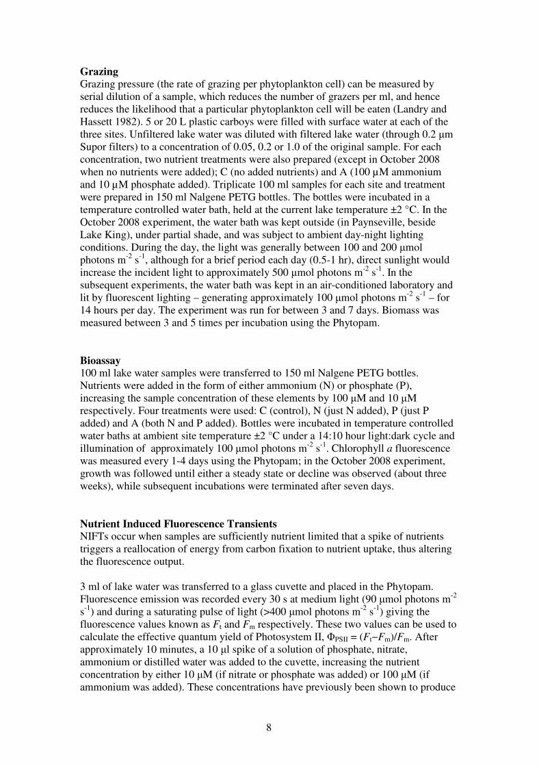
linear portion of the curve (see Figure 2). From these curves we also estimated the

irradiance where maximum photosynthesis occurred (in this case it was around 300-

400 µmol photons m-2

s-1

), and ran a separate experiment measuring the change in

dissolved oxygen (DO) in sealed 260 ml glass bottles over time either in the dark or at

saturating irradiance. From this we calculated the maximum photosynthesis rate

(Pmax), and then recalculated α as a function of this, rather than ETRmax.

light (I)

pho

tosyn

the

sis

(P

)

α

IkPmax

Figure 2. Stylised PI curve. Ik is the extrapolated irradiance where the linear portion of the

curve would reach the maximum photosynthesis rate (Pmax). α is the slope of this line (Ik/Pmax).

Benthic flux (from in situ chambers)

Benthic fluxes were measured using automated benthic chambers deployed in situ.

The chamber design has been previously described in detail (Pomc 2008). Briefly,

each chamber enclosed 10-15 L of water over an area of 0.07 m2. The chambers were

stirred with a paddle stirrer at a rate sufficient to create a diffusive boundary layer

thickness of 0.3-0.4 mm. The volume of the chamber was calculated from video

observation of the depth of penetration into the sediment. Two benthic chambers were

deployed at each site, and benthic fluxes were estimated by the change in

concentration of metabolites within the chambers over time. Both chambers were

transparent. Chambers were deployed for about 20 hours, and collected samples over

16 hours. All nutrient samples (NOx, NH4+, RP and RSi) were filtered (0.45 µm),

frozen in the field, and analysed at the Monash University Water Studies Centre using

10

standard colorimetric methods (Grasshoff 1983). Samples for pH were analysed in the

field using a high-precision electrode and meter. Alkalinity was estimated by Gran

titration of samples with dilute standardised HCl. Benthic fluxes were calculated by

linear least-squares regression of metabolite concentration over time; only linear

portions of the concentration/time plots were used to estimate fluxes.

Nitrogen cycling in the water column

Surface-water samples were collected from the each of the three sites; bottom water

was also collected in October 2008 only. 150 ml samples were incubated for 4-6

hours after the addition of 0.1 µM of either 15

NO3- or

15NH4

+. Samples were incubated

either in the light at between 100 and 200 µmol photons m-2

s-1

, or the dark. In

October 2008 surface water was used in the light and bottom water in the dark

incubations, and a second set of bottom samples from Lake Victoria were kept in low

light (~10 µmol photons m-2

s-1

). At other times, surface water was used for both light

and dark incubations. At the end of the experiment, the samples were filtered onto

ashed GF/F filters, and frozen. 15

N retained on the filter and thus incorporated into the

phytoplankton was measured using a stable isotope mass spectrometer at Griffith

University. N-uptake rates were calculated using the technique of Dugdale and

Wilkerson (1986).

11

Results and Discussion

Phytoplankton community

A comparison between chlorophyll a values measured with the Phytopam and those

measured by chlorophyll extraction showed that, while the correlations within each

sampling trip were generally quite good, the relationship was not 1:1 and changed

over time. To calibrate the fluorescence output we therefore multiplied each of the

chlorophyll a fluorescence measurements by the calibration factor shown in Figure 3

to estimate the true chlorophyll a. The correlation for October 2008 was poor. While

the exact reason cannot be ascertained we believe that there were some errors in the

spectroscopic analysis of the extracted chlorophyll, due to very low readings. This

was rectified for the latter trips by combining the triplicate bioassay samples onto one

filter.

y = 5.8821x

R² = 0.8247y = 2.9612x

R² = 0.9442

y = 1.2059x

R² = 0.9532

y = 1.007x

R² = 0.178

0

20

40

60

80

100

120

0 5 10 15 20 25 30

Ext

ract

ed

ch

loro

ph

yll

a(µ

g/L

)

Chlorophyll a fluorescence (µg/L)

Mar-10

Dec-09

Oct-09

Oct-08

Figure 3. Chlorophyll a fluorescence (calculated by the Phytopam) versus extracted chlorophyll

a. Note that the high chlorophyll a concentrations are from samples collected at the end of the

nutrient addition bioassay incubations.

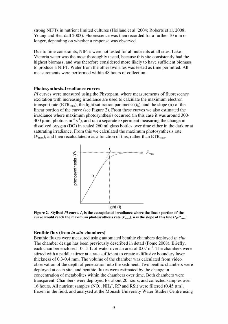
In October 2008, chlorophyll a was elevated at all three sites (background levels at

this time of year are typically 1-2 µg L-1

), and was highest in Lake Victoria, at almost

8 µg L-1

, which was twice as high as LKN, and 50% higher than LKS (Figure 4).

Chlorophyll a was considerably lower than this the following October and December

(0.5-4 µg L-1

), and by March 2010 it had increased to similar levels to those in

October 2008. Green algae dominated in October 2008, while brown algae (diatoms

and/or dinoflagellates) dominated at other times. Cyanobacteria were undetectable in

the majority of cases and a minor component of the flora in those cases where it was

detected.

12

0

1

2

3

4

5

6

7

8

9

N S V N S V N S V N S V

Oct-08 Oct-09 Dec-09 Mar-10

Ch

l a (

µg

/L

)

Brown

Green

Cyano

Figure 4. Chlorophyll a in the Gippsland Lakes, divided into Brown (diatoms and

dinoflagellates), Green (green algae) and Cyano (cyanobacteria), as measured by the Phytopam.

Bars labelled N represent LKN, S represents LKS and V represents LVC.

Grazing

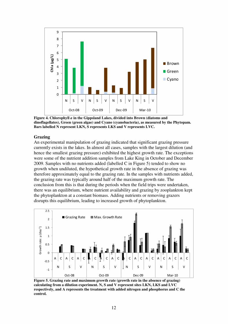
An experimental manipulation of grazing indicated that significant grazing pressure

currently exists in the lakes. In almost all cases, samples with the largest dilution (and

hence the smallest grazing pressure) exhibited the highest growth rate. The exceptions

were some of the nutrient addition samples from Lake King in October and December

2009. Samples with no nutrients added (labelled C in Figure 5) tended to show no

growth when undiluted, the hypothetical growth rate in the absence of grazing was

therefore approximately equal to the grazing rate. In the samples with nutrients added,

the grazing rate was typically around half of the maximum growth rate. The

conclusion from this is that during the periods when the field trips were undertaken,

there was an equilibrium, where nutrient availability and grazing by zooplankton kept

the phytoplankton at a constant biomass. Adding nutrients or removing grazers

disrupts this equilibrium, leading to increased growth of phytoplankton.

-1

-0.5

0

0.5

1

1.5

2

2.5

A C A C A C A C A C A C A C A C A C A C A C A C

N S V N S V N S V N S V

Oct-08 Oct-09 Dec-09 Mar-10

Gro

wth

ra

te:

µ (

da

y-1

)

Grazing Rate Max. Growth Rate

Figure 5. Grazing rate and maximum growth rate (growth rate in the absence of grazing)

calculating from a dilution experiment. N, S and V represent sites LKN, LKS and LVC

respectively, and A represents the treatment with added nitrogen and phosphorus and C the

control.

13

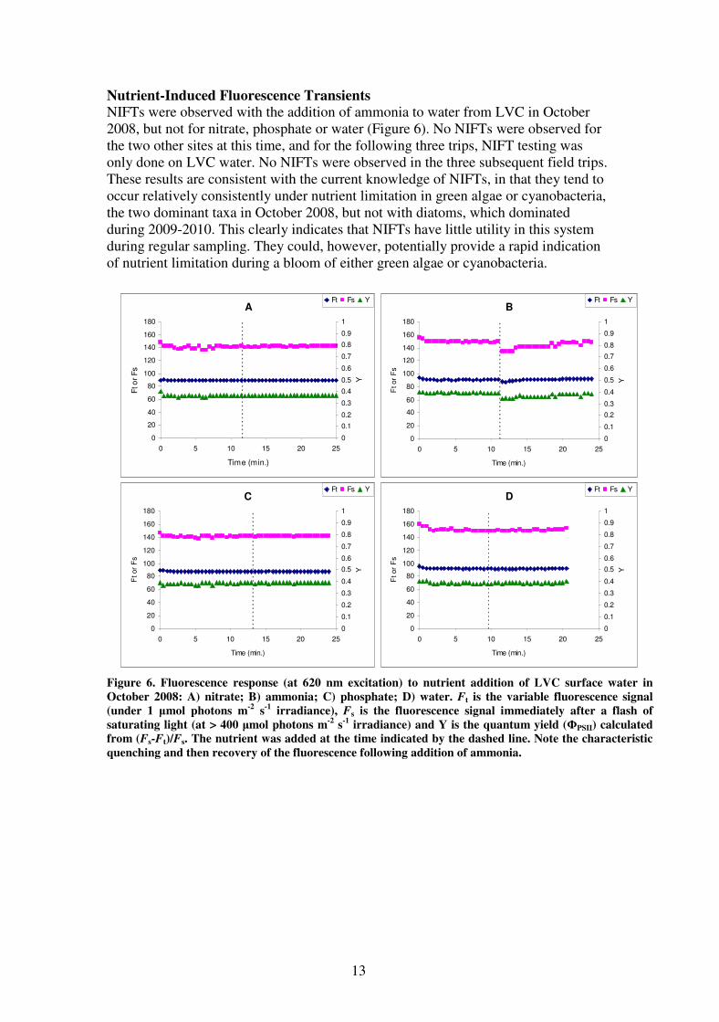
Nutrient-Induced Fluorescence Transients

NIFTs were observed with the addition of ammonia to water from LVC in October

2008, but not for nitrate, phosphate or water (Figure 6). No NIFTs were observed for

the two other sites at this time, and for the following three trips, NIFT testing was

only done on LVC water. No NIFTs were observed in the three subsequent field trips.

These results are consistent with the current knowledge of NIFTs, in that they tend to

occur relatively consistently under nutrient limitation in green algae or cyanobacteria,

the two dominant taxa in October 2008, but not with diatoms, which dominated

during 2009-2010. This clearly indicates that NIFTs have little utility in this system

during regular sampling. They could, however, potentially provide a rapid indication

of nutrient limitation during a bloom of either green algae or cyanobacteria.

A

0

20

40

60

80

100

120

140

160

180

0 5 10 15 20 25

Time (min.)

Ft o

r F

s

0

0.1

0.2

0.3

0.4

0.5

0.6

0.7

0.8

0.9

1

Y

Ft Fs Y

C

0

20

40

60

80

100

120

140

160

180

0 5 10 15 20 25

Time (min.)

Ft or

Fs

0

0.1

0.2

0.3

0.4

0.5

0.6

0.7

0.8

0.9

1

Y

Ft Fs Y

B

0

20

40

60

80

100

120

140

160

180

0 5 10 15 20 25

Time (min.)

Ft or

Fs

0

0.1

0.2

0.3

0.4

0.5

0.6

0.7

0.8

0.9

1

Y

Ft Fs Y

D

0

20

40

60

80

100

120

140

160

180

0 5 10 15 20 25

Time (min.)

Ft or

Fs

0

0.1

0.2

0.3

0.4

0.5

0.6

0.7

0.8

0.9

1

Y

Ft Fs Y

Figure 6. Fluorescence response (at 620 nm excitation) to nutrient addition of LVC surface water in

October 2008: A) nitrate; B) ammonia; C) phosphate; D) water. Ft is the variable fluorescence signal

(under 1 µmol photons m-2

s-1

irradiance), Fs is the fluorescence signal immediately after a flash of

saturating light (at > 400 µmol photons m-2

s-1

irradiance) and Y is the quantum yield (ΦPSII) calculated

from (Fs-Ft)/Fs. The nutrient was added at the time indicated by the dashed line. Note the characteristic

quenching and then recovery of the fluorescence following addition of ammonia.

14

Photosynthesis-Irradiance curves

The gross oxygen production rate of the surface water was calculated from the

difference between the rate of DO change in high (saturating) light and no light. The

rates were generally highest when the biomass was highest, e.g. in October 2008

(Figure 7).

The other PI parameters were similar among sites (apart from two unusually high

values, which cannot be explained and are probably due to measurement errors). The

samples had maximum photosynthesis rates at an irradiance of 300-400 µmol photons

m-2

, and values of the light saturation parameter, Ik (see Figure 2 for definition) were

high, generally >170 µmol photons m-2

, indicating that these populations were

adapted to high light. These results indicate that light is not likely to be a limiting

factor in phytoplankton growth in the surface waters of the lakes.

Bioassay

The October 2008 bioassay was run for 21 days, whereas the other three bioassays

were run for 7 days. For this report, therefore, the results of this first bioassay have

been re-analysed using only the first 10 days of measurements (no reading was taken

on day 7).

Similar results were observed for the three sites (Figure 8). In all cases, the full

nutrient treatment (nitrogen plus phosphorus) had the highest growth rate. This shows

that nutrients were limiting growth in this system, assuming the in situ growth

conditions matched the experimental conditions. There was no significant difference

between the control and phosphorus treatments in any of the bioassays. Nitrogen

treatments generally had higher growth rates than the controls, but lower than the full

treatment. Combined, this data indicates that at the time these waters were collected,

N was more limiting than P, but that both were in short supply. The phytoplankton

appear to be able to adapt to an increase in N (through either changes in the

population structure or cellular nutrient content) but not to P. The data also suggests

that little or no nitrogen fixation was occurring in the water column at these times, in

agreement with the lack of cyanobacteria.

15

Figure 7. Photosynthetic parameters at each site over time. N, S and V represent sites LKN, LKS

and LVC respectively.

16

-0.2

-0.15

-0.1

-0.05

0

0.05

0.1

0.15

0.2

C P N A C P N A C P N A

N S V

Gro

wth

(/d

ay)

Site and nutrient addition

Oct-08

-0.4

-0.2

0

0.2

0.4

0.6

0.8

1

C P N A C P N A C P N A

N S V

Gro

wth

(/d

ay)

Site and nutrient addition

Oct-09

0

0.2

0.4

0.6

0.8

1

1.2

1.4

1.6

C P N A C P N A C P N A

N S V

Gro

wth

(/d

ay)

Site and nutrient addition

Dec-09

-0.6

-0.4

-0.2

0

0.2

0.4

0.6

0.8

1

1.2

1.4

C P N A C P N A C P N A

N S V

Gro

wth

(/d

ay)

Site and nutrient addition

Mar-10

Figure 8. Results of nutrient enrichment bioassays conducted on Gippsland Lakes surface water

samples. N, S and V represent sites LKN, LKS and LVC respectively, and A represents the

treatment with added nitrogen and phosphorus and C the control. Results include standard error

bars.

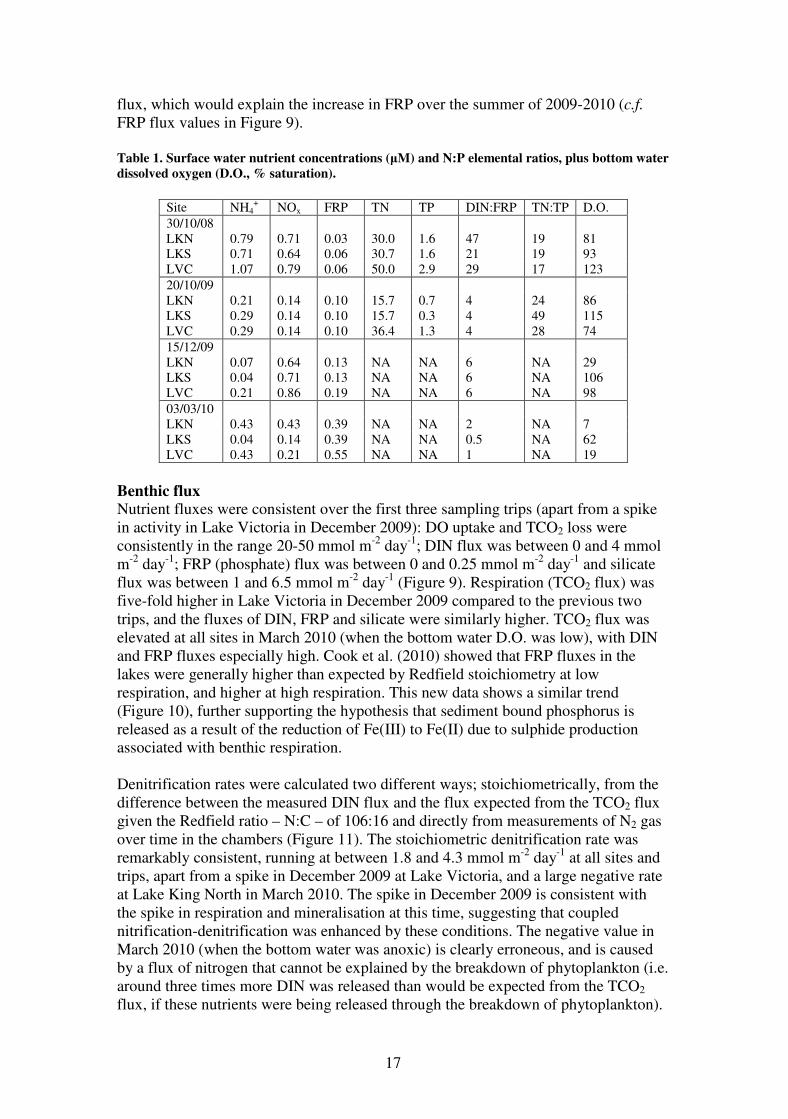
Water column nutrients

Dissolved inorganic nitrogen (DIN, NH4+ and NOx) was elevated in October 2008, at

between 1.3 and 2 µM (Table 1). This elevation in DIN was a result of the floods of

June 2007. These nitrogen levels had been declining as time went by, and in our

previous report we predicted that denitrification would remove this excess DIN by

early in 2009. By October 2009, DIN had dropped to around 0.4 µM, a more typical

value for the lakes, when not influenced by floods. In December 2009 and March

2010 DIN values were slightly higher, at around 0.7 µM. FRP was higher at each

successive sampling trip, rising from almost undetectable, at 0.03-0.06 µM in October

2008, to >0.4 µM in March 2010. DIN:FRP was higher than the Redfield ratio in

October 2008, but was very low during the other field trips (Table 1). On their own,

these results would suggest that phosphorus was limiting in October 2008, whereas

nitrogen was limiting at the other times. Total Nitrogen (TN) and Total Phosphorus

(TP) were measured during the first two field trips; the values were much higher than

the inorganic nitrogen and phosphorus and the ratio was only slightly higher than the

Redfield ratio (Table 1). Bottom water dissolved oxygen was close to saturation,

except at LKN in December 2009 and in March 2010, when all sites had low D.O.,

particularly LKN and LVC. These low D.O. values could be indicative of high FRP

17

flux, which would explain the increase in FRP over the summer of 2009-2010 (c.f.

FRP flux values in Figure 9).

Table 1. Surface water nutrient concentrations (µM) and N:P elemental ratios, plus bottom water

dissolved oxygen (D.O., % saturation).

Site NH4

+ NOx FRP TN TP DIN:FRP TN:TP D.O.

30/10/08

LKN 0.79 0.71 0.03 30.0 1.6 47 19 81

LKS 0.71 0.64 0.06 30.7 1.6 21 19 93

LVC 1.07 0.79 0.06 50.0 2.9 29 17 123

20/10/09

LKN 0.21 0.14 0.10 15.7 0.7 4 24 86

LKS 0.29 0.14 0.10 15.7 0.3 4 49 115

LVC 0.29 0.14 0.10 36.4 1.3 4 28 74

15/12/09

LKN 0.07 0.64 0.13 NA NA 6 NA 29

LKS 0.04 0.71 0.13 NA NA 6 NA 106

LVC 0.21 0.86 0.19 NA NA 6 NA 98

03/03/10

LKN 0.43 0.43 0.39 NA NA 2 NA 7

LKS 0.04 0.14 0.39 NA NA 0.5 NA 62

LVC 0.43 0.21 0.55 NA NA 1 NA 19

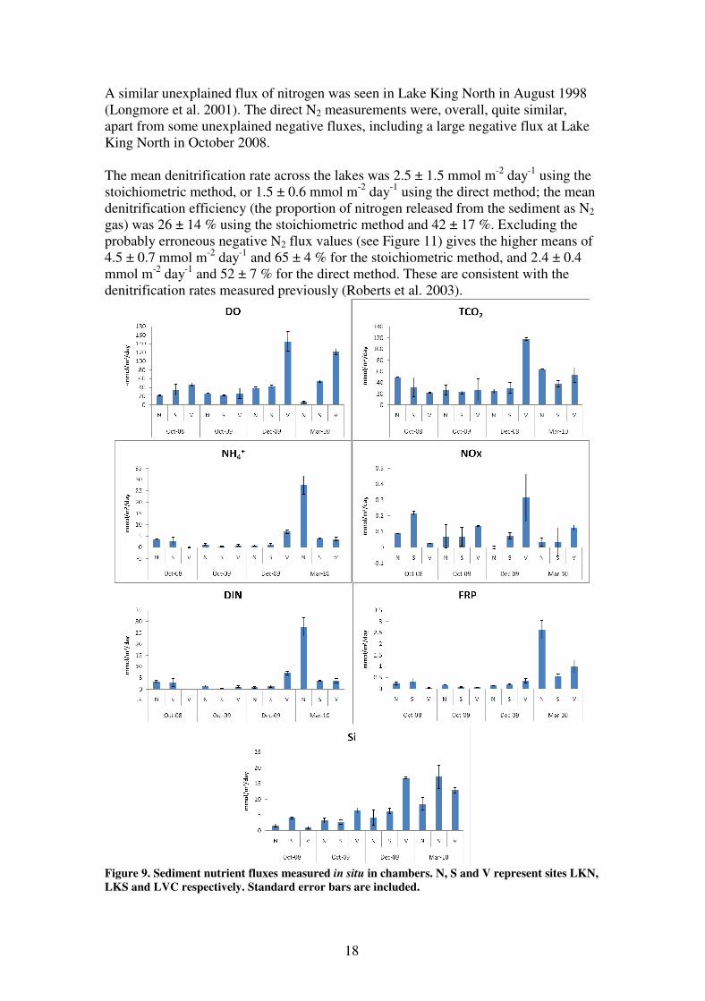
Benthic flux

Nutrient fluxes were consistent over the first three sampling trips (apart from a spike

in activity in Lake Victoria in December 2009): DO uptake and TCO2 loss were

consistently in the range 20-50 mmol m-2

day-1

; DIN flux was between 0 and 4 mmol

m-2

day-1

; FRP (phosphate) flux was between 0 and 0.25 mmol m-2

day-1

and silicate

flux was between 1 and 6.5 mmol m-2

day-1

(Figure 9). Respiration (TCO2 flux) was

five-fold higher in Lake Victoria in December 2009 compared to the previous two

trips, and the fluxes of DIN, FRP and silicate were similarly higher. TCO2 flux was

elevated at all sites in March 2010 (when the bottom water D.O. was low), with DIN

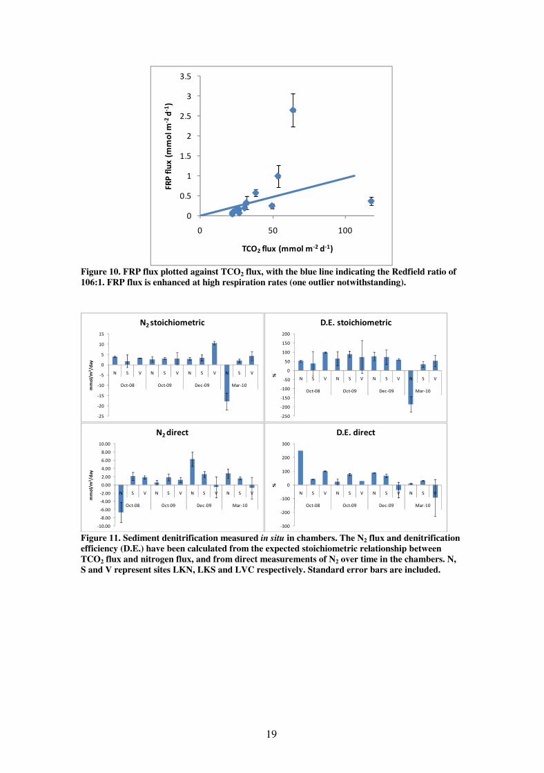
and FRP fluxes especially high. Cook et al. (2010) showed that FRP fluxes in the

lakes were generally higher than expected by Redfield stoichiometry at low

respiration, and higher at high respiration. This new data shows a similar trend

(Figure 10), further supporting the hypothesis that sediment bound phosphorus is

released as a result of the reduction of Fe(III) to Fe(II) due to sulphide production

associated with benthic respiration.

Denitrification rates were calculated two different ways; stoichiometrically, from the

difference between the measured DIN flux and the flux expected from the TCO2 flux

given the Redfield ratio – N:C – of 106:16 and directly from measurements of N2 gas

over time in the chambers (Figure 11). The stoichiometric denitrification rate was

remarkably consistent, running at between 1.8 and 4.3 mmol m-2

day-1

at all sites and

trips, apart from a spike in December 2009 at Lake Victoria, and a large negative rate

at Lake King North in March 2010. The spike in December 2009 is consistent with

the spike in respiration and mineralisation at this time, suggesting that coupled

nitrification-denitrification was enhanced by these conditions. The negative value in

March 2010 (when the bottom water was anoxic) is clearly erroneous, and is caused

by a flux of nitrogen that cannot be explained by the breakdown of phytoplankton (i.e.

around three times more DIN was released than would be expected from the TCO2

flux, if these nutrients were being released through the breakdown of phytoplankton).

18

A similar unexplained flux of nitrogen was seen in Lake King North in August 1998

(Longmore et al. 2001). The direct N2 measurements were, overall, quite similar,

apart from some unexplained negative fluxes, including a large negative flux at Lake

King North in October 2008.

The mean denitrification rate across the lakes was 2.5 ± 1.5 mmol m-2

day-1

using the

stoichiometric method, or 1.5 ± 0.6 mmol m-2

day-1

using the direct method; the mean

denitrification efficiency (the proportion of nitrogen released from the sediment as N2

gas) was 26 ± 14 % using the stoichiometric method and 42 ± 17 %. Excluding the

probably erroneous negative N2 flux values (see Figure 11) gives the higher means of

4.5 ± 0.7 mmol m-2

day-1

and 65 ± 4 % for the stoichiometric method, and 2.4 ± 0.4

mmol m-2

day-1

and 52 ± 7 % for the direct method. These are consistent with the

denitrification rates measured previously (Roberts et al. 2003).

Figure 9. Sediment nutrient fluxes measured in situ in chambers. N, S and V represent sites LKN,

LKS and LVC respectively. Standard error bars are included.

19

0

0.5

1

1.5

2

2.5

3

3.5

0 50 100

FR

P f

lux

(m

mo

l m

-2d

-1)

TCO2 flux (mmol m-2 d-1)

Figure 10. FRP flux plotted against TCO2 flux, with the blue line indicating the Redfield ratio of

106:1. FRP flux is enhanced at high respiration rates (one outlier notwithstanding).

-25

-20

-15

-10

-5

0

5

10

15

N S V N S V N S V N S V

Oct-08 Oct-09 Dec-09 Mar-10

mm

ol/

m2/

da

y

N2 stoichiometric

-250

-200

-150

-100

-50

0

50

100

150

200

N S V N S V N S V N S V

Oct-08 Oct-09 Dec-09 Mar-10

%

D.E. stoichiometric

-10.00

-8.00

-6.00

-4.00

-2.00

0.00

2.00

4.00

6.00

8.00

10.00

N S V N S V N S V N S V

Oct-08 Oct-09 Dec-09 Mar-10

mm

ol/

m2/

da

y

N2 direct

-300

-200

-100

0

100

200

300

N S V N S V N S V N S V

Oct-08 Oct-09 Dec-09 Mar-10

%

D.E. direct

Figure 11. Sediment denitrification measured in situ in chambers. The N2 flux and denitrification

efficiency (D.E.) have been calculated from the expected stoichiometric relationship between

TCO2 flux and nitrogen flux, and from direct measurements of N2 over time in the chambers. N,

S and V represent sites LKN, LKS and LVC respectively. Standard error bars are included.

20

Nitrogen cycling in the water column

The uptake rate of 15

N from labelled ammonia or nitrate provides a measure of the

nitrogen cycling within the water column. Uptake, which is an energy requiring

process, was, as expected, greater in the light than the dark, and the average of these

gives a rough estimation of daily uptake (Figure 12). Uptake of nitrate was higher

than the uptake of ammonia in October 2008, with the reverse occurring at the other

three times. Uptake was higher in October 2008 and December 2009 than at the other

two times.

0

2

4

6

8

10

12

14

16

18

20

N S V N S V N S V N S V

Oct-08 Oct-09 Dec-09 Mar-10

mm

ol/

m2/

da

y

Ammonia

Nitrate

Figure 12. Daily uptake of

15N-labelled ammonia and nitrate integrated through the water

column (with standard error bars). N, S and V represent sites LKN, LKS and LVC respectively.

21

General discussion

Lake Wellington used to be dominated by macrophytes, but a drought in 1968 led to

an influx of saline water from Lake Victoria, which killed these plants. The lake never

recovered, and has since been dominated by phytoplankton (Harris et al. 1988). The

Synechococcus bloom in lakes Victoria and King severely reduced light penetration

and there were anecdotal reports of seagrass loss, and subsequent measurements

showed a reduction in seagrass cover compared with 10 years previously (Hindell and

Warry 2009). The concern was that this could provide a similar “tipping point” to

what occurred in Lake Wellington, consigning the entire Lakes Victoria and King

region to a long period dominated by nanoplankton with a concomitant reduction in

important habitats. It is now apparent that while the effect of fires and floods was

quite significant during late 2007 and 2008, leading to this widespread and persistent

phytoplankton bloom, this impact has now subsided. When the seagrass was

resampled in April 2009, significant recovery was seen, and in the October 2009 to

March 2010 field season for this study, the lakes had returned to what we would

consider to be typical, low flow, pre-Synechococcus conditions. These conditions

include relatively low dissolved nutrient concentrations and nitrogen limitation of

phytoplankton growth.

Nitrogen

The year from 1 June 2007 – 31 May 2008 saw the introduction of an unprecedented

6060 tonnes of nitrogen into the Gippsland Lakes – more than four times the annual

average for the previous 20 years, and twice the next highest load. The major

mechanism for nitrogen removal in the Gippsland Lakes is likely to be through

denitrification within the sediments (Webster et al. 2001). The mean denitrification

rate measured in the current study was 2.5 mmol m-2

day-1

, or ~13 tonnes day-1

(based

on a lakes-wide surface area of 364 km2), which would have removed this nitrogen in

around 470 days. We note that this estimate of denitrification is biased by the fact that

it was measured at the deep sites within the lakes. In 2002, DIN fluxes were

measured in both shallow and deep chambers, and the deep sites had more than four

times the fluxes than the shallow sites (6.2 mmol m-2

day-1

compared with 1.4 mmol

m-2

day-1

). This is likely a result of lower organic loading to these shallow sites, and

pore water analysis suggests that this is the case – Longmore (2000) found 118 mmol

m-2

ammonia in the top 20 cm of pore water in deep water sites compared with 38

mmol m-2

in shallow sites. If we assume that denitrification efficiency is the same

across the lakes, we can estimate that shallow sites will have an average

denitrification rate close to 0.6 mmol m-2

day-1

. Given that all of Lake Wellington, all

of Jones Bay and the western third of Lake Victoria – representing more than half of

the surface area of the lakes – are < 4 m deep (estimated from Fig. 2.2 in Webster et

al. 2001), a realistic average lake-wide denitrification rate is probably somewhere

between the deep and shallow values; the average of these is 1.6 mmol m-2

day-1

, i.e. 8

tonnes day-1

. This rate would increase the time taken to remove the 6060 tonnes of

nitrogen to around 760 days. Denitrification within the lakes, therefore, has the

capacity to remove a substantial fraction of catchment derived nitrogen, even in years

of extreme loading.

One of the critical questions to be investigated by this study is whether or not the

2007 flood and subsequent Synechococcus bloom affected denitrification rates. We

hypothesised that the small Synechococcus cells would not sink, therefore slowing the

22

rate of nitrogen supply to the sediment, and hence the rate of N removal through

denitrification. Denitrification rates were not measured during the bloom itself, but

inspection of in-lake TN in the water column at Lake King South shows that total

nitrogen concentrations remained elevated in the water column of the Gippsland

Lakes for much longer than a previous comparable flood in 1999 (Figure 13). Total N

concentrations, did, however, return to the long term baseline concentration of ~20-30

µM by the summer of 2009-2010 (Figure 13). This steady decline in TN back to

baseline conditions closely matches the trend expected from the denitrification rates.

Date

Jan 06 Jan 07 Jan 08 Jan 09 Jan 10 Jan 11

Tota

l N

itro

gen

(µM

)

0

20

40

60

80

100

120

Date

Jan 97 Jan 98 Jan 99 Jan 00 Jan 01 Jan 02

2006-2011

1997-2002

Flood

Figure 13. Comparison of surface water total nitrogen concentrations for the period 1997-2002

(top axis) and 2006-2011 (bottom axis). A flood occurred in the middle of the second year in each

range, leading to a spike in nitrogen levels. The peak in March 1999 was the result of a Nodularia

bloom, while the high levels throughout 2008 track the Synechoccocus bloom.

Measurements of benthic respiration (TCO2 flux), SiO4 fluxes and denitrification all

suggest benthic recycling rates and processes are not markedly altered from those

prior to 2007 (Table 2). The delivery of organic material to the sediment in 2008-2009

and 2009-2010 (as indicated by the TCO2 fluxes) is remarkably consistent with rates

measured previously at similar sites. Diatoms are generally thought to be an

important vector for carbon delivery to the sediment because of their relatively rapid

sinking velocity, and we can use SiO4 fluxes as a tracer for their importance (Haese et

al. 2007). The recent SiO4 fluxes and the TCO2:SiO4 flux ratios in Table 2 are within

the range of those observed prior to 2007, suggesting that the importance of diatoms

as a vector for organic carbon delivery to the sediment remains unaltered. Consistent

with these observations, denitrification rates within the sediment (both in terms of the

absolute amount of nitrogen and the efficiency of the process) are not markedly

different to prior to the 2007 flood event.

23

Table 2. Mean (+S.E.) fluxes and denitrification rates (mmol m-2

day-1

) calculated by

stoichiometric balance or direct measurement of fluxes (in chambers). Denitrification Efficiency

(D.E.) calculated from the stoichiometric technique.

Date Site TCO2 flux SiO4 flux TCO2:SiO4 Denit.

(stoich)

Denit.

(measured)

D.E.

N 36 ± 16 1.6 ± 0.6 23 ± 14 2.4 ± 1.8 71 ± 10

S 83 ± 21 2.8 ± 0.8 30 ± 11 10.3 ± 3.6 63 ± 12

V 2 ± 17 1.8 ± 0.7 1 ± 10 -0.7 ± 2.5 83 ± 10

1997-98

Average 39 ± 12 2.0 ± 0.4 19 ± 7 3.9 ± 1.7 73 ± 6

N 25 ± 14 3.3 ± 0.4 7 ± 4 -1.3 ± 1.9 21 ± 29

S 48 ± 8 3.9 ± 0.3 12 ± 2 2.6 ± 0.8 32 ± 9

V 47 ± 7 7.1 ± 1.1 7 ± 1 2.3 ± 0.7 18 ± 16 1998-99

Average 40 ± 6 4.8 ± 0.4 8 ± 1 1.2 ± 0.8 24 ± 11

N 65 ± 22 5.0 ±1.4 13 ± 6 5.2 ± 2.1 4.2 ± 1.4 49 ± 7

S 30 ± 5 3.2 ± 0.6 9 ± 2 2.6 ± 1.3 4.6 ± 1.2 26 ± 28

V 85 ± 14 8.1 ± 1.2 10 ± 2 4.8 ± 1.2 4.0 ± 1.2 40 ± 7

2002-03

Average 64 ± 9 5.9 ± 0.8 11 ± 2 4.2 ± 0.8 4.2 ± 0.8 38 ± 9

N 49 ± 1 1.7 ± 0.5 30 ± 9 7.7 ± 1.3 -6.7 ± 0 70 ± 8

S 32 ± 17 4.1 ± 0.3 8 ± 4 2.7 ± 0.6 2.1 ± 1.0 51 ± 20

V 22 ± 0.5 1.0 ± 0.5 22 ± 9 8.0 ± 2.0 1.8 ± 0.4 100 ± 0

2008-09

Average 35 ± 7 2.3 ± 0.6 15 ± 5 6.2 ± 1.3 0.3 ± 1.8 74 ± 11

N 39 ± 8 6.2 ± 1.4 6 ± 2 -4.1 ± 4.5 3.6 ± 1.1 -15 ± 55

S 31 ± 4 8.7 ± 2.9 3 ± 1 2.8 ± 0.4 2.0 ± 0.3 65 ± 10

V 66 ± 18 13.1 ± 1.8 5 ± 2 5.4 ± 1.9 -0.0 ± 1.0 39 ± 14 2009-10

Average 46 ± 8 9.2 ± 1.5 5 ± 1 1.3 ± 1.9 1.8 ± 0.6 28 ± 21

Finally, we calculate a rough snapshot of nitrogen movement for each of the field

trips (Figure 14). For each trip in Figure 14 we have presented both the high load year

of 2007-2008 and the low load year 2008-2009, and the subsequent net nitrogen gain

(or loss) from the system based on these extremes. This has been done because

nitrogen loads enter the system in bursts over a long period, while the flux and

recycling rates that are presented are from a single moment in time. These

approximations show that in low flow years there is likely to be an overall loss of

nitrogen from the system (a negative net gain of N), and in high flow years there is

potential for a net gain of N. Overall, it seems that denitrification has the potential to

remove all of the nitrogen inputs in an average year. Nitrogen recycling was an order

of magnitude greater in the water column than in the sediment, except in March 2010,

where DIN flux rates appear to be higher than water column nitrogen uptake rates;

this suggests a net increase in water column DIN at this time.

24

catchment

benthos

atmosphere

se

ttling

(5.2

)

flux (2

.2)

de

nitrific

atio

n (3

.0)

recycling(21.4)

Oct 2008

flow (0.4-3.3)

Net N gain = -2.4-0.3

catchment

benthos

atmosphere

se

ttling

(3.8

)

flux (0

.9)

de

nitrific

atio

n (2

.9)

recycling(6.6)

Oct 2009

flow (0.4-3.3)

Net N gain = -2.5-0.4

catchment

benthos

atmosphere

se

ttling

(8.7

)

flux (3

.1)

de

nitrific

atio

n (5

.6)

recycling(21.3)

Dec 2009

flow (0.4-3.3)

Net N gain = -5.2 to -2.2

catchment

benthos

atmosphere

flow (0.4-3.3)

se

ttling

(14

.8)

flux (1

1.7

)

de

nitrific

atio

n (3

.1)

recycling(-3.6)

Mar 2010

Net N gain = -2.7-0.2

Figure 14. Nitrogen budgets for the Gippsland Lakes based on recycling, flux and denitrification

rates calculated at the given date, and the minimum and maximum annual nitrogen loads for the

period 2007-2009.The denitrification rate for March 2010 neglects the rate calculated for Lake

King North as this leads to an unrealistic value of -3.9 mmol m-2

day-1

. Recycling rates are the

nitrogen uptake rates minus the DIN flux rates; the negative recycling rate in March 2010 may

indicate a disequilbrium between benthic flux and uptake at this time.

Phosphorus

The ultimate fate of phosphorus in the lakes is either to be buried in the sediment or to

move out to the ocean. This makes phosphorus a much more persistent element, and

hence has been of greater concern to managers of the Gippsland Lakes. The

hydrologic year 1 June 2007 – 31 May 2008 saw the introduction of 870 Tonnes of

phosphorus into the Gippsland Lakes, while the average annual input in the 20 years

previous to this was 156 Tonnes.

FRP fluxes from the sediment were relatively low in the first three field trips, but

were higher in March 2010, in agreement with the higher water column

concentrations. It has been demonstrated that the sediment is the primary source of

phosphorus for Nodularia blooms (Cook et al. 2010), and so the large addition of

phosphorus in 2007-2008 (now in the sediment) may be available for future blooms if

the right conditions occur. The results of this study in combination with our previous

studies suggest that high respiration leads to increased phosphorus flux, so it may be

that another winter flood, followed by a diatom and/or dinoflagellate bloom followed

by a calm summer will lead to the mobilisation of this extra phosphorus, potentially

increasing the magnitude of the Nodularia bloom.

Phytoplankton Growth – Bloom potential

From October 2009-March 2010 Lakes King and Victoria were once again

dominated by low to moderate levels of diatoms and dinoflagellates, as they tend to

be outside of cyanobacterial algal blooms. At the times that these experiments were

25

run, there was an equilibrium between nutrient supply and grazing, such that

phytoplankton biomass was constant. The experimental addition of nitrogen and

phosphorus led to an increase in both the growth rate and of the grazing rate, but

under nutrient replete conditions the growth rate outpaced the grazing rate by

approximately 2:1. Presumably over time the grazers would further adapt to the

increased growth and the grazing rate would again balance or exceed the growth rate,

but it is clear that influxes of nutrients give the phytoplankton a head start. It thus

appears likely that bottom-up processes (benthic flux and nutrient loads) are the key

drivers of bloom potential in this system, although top-down processes such as

grazing may have the effect of minimizing the size and duration of blooms.

High rates of water column nitrogen recycling will prolong a bloom by reducing the

supply of nutrients to the sediment, where denitrification occurs. The rates measured

in this study provide a basis for future comparisons with recycling rates that could be

measured during blooms of various taxa, such as diatoms, dinoflagellates,

Synechococcus and Nodularia, which may then provide further insights into the

dynamics of such blooms, and the overall biogeochemical processing within the lakes.

Risk of a Synechococcus bloom

It is clear that Synechococcus is, and will remain, a part of the phytoplankton

community in the Gippsland Lakes. While it is difficult to draw conclusions from a

single event, it is apparent that there is a risk of further Synechococcus blooms if

conditions similar to those that occurred in 2007-2008 recur. Given that this bloom

was sustained by large amounts of DIN, and that in a typical year most, if not all of

the DIN that enters the lakes is removed via denitrification, then it will take another

massive influx of nitrogen to initiate a similar bloom. The only possible avenue for

this is influx is the combination of widespread fires followed by widespread flooding.

Risk of a Nodularia bloom

The evidence suggests that the lakes have returned to the point that they were prior to

the fires and floods of 2007. The risk factors for Nodularia blooms therefore remain

where they have been for the last 20-30 years, with one potential further risk: the fate

of the massive load of phosphorus that entered the lakes following the bushfires is

unknown. Any phosphorus held in the water column will slowly be removed via

exchange with Bass Straight, but this is likely to be a slow process, and most of the

phosphorus will instead be sediment bound, or dissolved in the pore water. This is

therefore an additional source of phosphorus to that which was available prior to the

fires, and may exacerbate any Nodularia blooms that occur in the near future.

Management implications and climate change

If the Gippsland Lakes become a marine dominated system, which could occur

through a combination of rising sea levels and reduced freshwater inflows, this will

clearly have implications for the future risk of algal blooms. Historically, Nodularia

blooms occur when the lake surface water salinity is between 15 and 20 (Cook et al.

2008), and these conditions, along with suitable temperature, light and nutrients, will

be unlikely to occur very often under this future scenario, where the salinity will be

close to twice this range. There may be an increased risk of blooms of other,

potentially problematic species under this scenario, but analyses of these possibilities

is beyond the scope of the current study.

26

Denitrification efficiently removes nitrogen from the lakes, and is probably a key

factor in keeping the lakes from becoming permanently hypereutrophic, such as they

were following the fires and flood of 2006-2007, when the Synechococcus bloom

occurred. The bottom waters of the lakes are already largely marine, and further

changes in this direction are unlikely to change the denitrification potential of this

system, although we advise vigilant monitoring.

While phosphorus is the nutrient that limits Nodularia bloom formation, our recent

research found, somewhat ironically, that it is the nitrogen load that provides the

initial trigger for a string of processes ultimately leading to a mass release of

phosphorus from the sediment. Therefore, while long-term steps to reduce the load of

phosphorus to the lakes will ultimately reduce the sediment phosphorus pool, these

steps will have little effect in the short-medium term, and there is the risk that

bushfires, which are inevitable, and likely to occur more frequently in the future, will

negate any reduction in baseline phosphorus inputs. It may therefore be necessary to

focus nutrient-reduction strategies on nitrogen as well as phosphorus.

27

References Beardall, J. 2008. Blooms of Synechococcus: An analysis of the problem worldwide and possible

causative factors in relation to nuisance blooms in the Gippsland Lakes. Monash University.

Cook, P. L. M., D. P. Holland, and A. R. Longmore. 2008. Interactions between phytoplankton

dynamics, nutrient loads and the biogeochemistry of the Gippsland Lakes. Monash University,

http://www.gippslandlakestaskforce.vic.gov.au/.

---. 2010. Effect of a flood event on the dynamics of phytoplankton and biogeochemistry in a large

temperate Australian lagoon. Limnology and Oceanography 55: 1123-1133.

Dugdale, R. C., and F. P. Wilkerson. 1986. The use of 15

N to measure nitrogen uptake in eutrophic

oceans; experimental considerations. Limnology and Oceanography 31: 673-689.

Grasshoff, K. 1983. Methods of Seawater Analysis, 2nd edition. Verlag Chemie.

Haese, R. R., E. J. Murray, C. S. Smith, J. Smith, L. Clementson, and D. T. Heggie. 2007. Diatoms

control nutrient cycles in a temperate, wave-dominated estuary (southest Australia).

Limnology and Oceanography 52: 2686-2700.

Harris, G., G. Batley, I. T. Webster, R. Molloy, and D. Fox. 1988. Gippsland Lakes Environmental

Audit: Review of water quality and status of the aquatic ecosystems of the Gippsland Lakes.

CSIRO.

Hindell, J. S., and F. Y. Warry. 2009. Fish assemblages and seagrass condition of the Gippsland lakes.

p. 43. Arthur Rylah Instiute for Environmental Research, Victorian Department of

Sustainability and Environment.

Holland, D. P., P. Cook, J. Beardall, and A. Longmore. 2009. Gippsland Lakes 'Snapshot' - nutrient

cycling and phytoplankton population dynamics. Monash University Water Studies Centre.

Holland, D. P., S. C. Roberts, and J. Beardall. 2004. Assessment of the nutrient status of phyoplankton:

a comparison between conventional bioassays and nutrient-induced fluorescence transients

(NIFTs). Ecological Indicators 4: 149-159.

Howarth, R. W., R. Marino, and J. J. Cole. 1988. Nitrogen fixation in freshwater, estuarine, and marine

ecosystems. 2. Biogeochemical controls. Limnology and Oceanography 33: 688-701.

Jakob, T., U. Schreiber, V. Kirchesch, U. Langner, and C. Wilhelm. 2005. Estimation of chlorophyll

content and daily primary production of the major algal groups by means of multiwavelength-

excitation PAM chlorophyll fluorometry: performance and methodological limits.

Photosynthesis Research 83: 343-361.

Landry, M. R., and R. P. Hassett. 1982. Estimating the grazing impact of marine micro-zooplankton.

Marine Biology 67: 283-288.

Longmore, A. R. 2000. Gippsland Lakes sediment nutrient inventory., Marine and Freshwater

Resources Institute Report No. 21. Fisheries Victoria, Victoria, Australia.

Longmore, A. R., G. J. Nicholson, and B. Abbot. 2001. Effects of water quality on black bream habitat

in the Gippsland Lakes. p. 87. Marine and Freshwater Resources Institute.

Marino, R., F. Chan, R. W. Howarth, M. Pace, and G. E. Likens. 2002. Ecological and biogeochemical

interactions constrain planktonic nitrogen fixation in estuaries. Ecosystems 5: 719-725.

Marino, R., F. Chan, R. W. Howarth, M. L. Pace, and G. E. Likens. 2006. Ecological constraints on

planktonic nitrogen fixation in saline estuaries. I. Nutrient and trophic controls. Marine

Ecology-Progress Series 309: 25-39.

Moisander, P. H., and H. W. Paerl. 2000. Growth, primary productivity, and nitrogen fixation potential

of Nodularia spp. (cyanophyceae) in water from a subtropical estuary in the United States.

Journal of Phycology 36: 645-658.

Pomc. 2008. Nutrient cycling (denitrification) - detailed design - CDP ENV MD 019 Rev 1.

www.channelproject.com. Port of Melbourne Corporation.

Roberts, S., B. T. Hart, D. P. Holland, A. Longmore, G. Nicholson, and B. Light. 2003. Algal blooms

in the Gippsland Lakes: Assessment of the importance of sediment-bound nutrients. Technical

report fo Coast and Clean Seas project.

Roberts, S., K. Shelly, and J. Beardall. 2008. Interactions among phosphate uptake, photosynthesis, and

chlorophyll fluorescence in nutrient-limited cultures of the chlorophyte microalga Dunaliella

tertiolecta. Journal of Phycology 44: 662-669.

Stephens, A., N. Biggins, and S. Brett. 2004. Algal bloom dynamics in the estuarine Gippsland Lakes.

Victorian Environmental Protection Agency.

Webster, I. T., J. S. Parslow, R. B. Grayson, R. P. Molloy, J. Andrewartha, P. Sakov, K. S. Tan, S. J.

Walker, and B. B. Wallace. 2001. Gippsland Lakes Environmental Study: Assessing options

28

for improving water quality and ecological function. Gippsland Lakes Environmental Study.

CSIRO.

Young, E. B., and J. Beardall. 2003. Rapid ammonium- and nitrate-induced perturbations to chl a

fluorescence in nitrogen-stressed Dunaliella tertiolecta (Chlorophyta). Journal of Phycology

39: 332-342.