An ESRC Research Group Nutritional status and economic development in sub-Saharan Africa, 1950-1980 GPRG-WPS-046 Alexander Moradi Global Poverty Research Group Website: http://www.gprg.org/ The support of the Economic and Social Research Council (ESRC) is gratefully acknowledged. The work was part of the programme of the ESRC Global Poverty Research Group.
Transcript
An ESRC Research Group
Nutritional status and economic development in sub-Saharan Africa, 1950-1980
GPRG-WPS-046
Alexander Moradi
Global Poverty Research Group
Website: http://www.gprg.org/
The support of the Economic and Social Research Council (ESRC) is gratefully acknowledged. The work was part of the
programme of the ESRC Global Poverty Research Group.
1
12/07/06
Nutritional status and economic development in sub-Saharan Africa, 1950-1980
Alexander Moradi Centre for the Study of African Economies
Department of Economics, University of Oxford Postal address: Manor Road Building, Oxford OX1 3UQ, UK
Keywords: nutrition, health, anthropometry, living standards, sub-Saharan Africa JEL: I10, I30, N37 Word count: 9323 Acknowledgements I thank Joerg Baten, Gerhard Kling, John Komlos, Marco Sunder, and participants of the Economics and Human Biology Conference and CSAE Conference on Reducing Poverty and Inequality for helpful comments on earlier versions. I am also grateful for access to the Demographic and Health Survey database, kindly provided by Macro International, and especially to Stephan Klasen for his idea to use the DHS height data by birth cohorts.
2
Nutritional status and economic development in sub-Saharan Africa, 1950-1980
Abstract
Nutrition and health are important dimensions of human well-being. Both aspects are
complementary to income and deserve attention in its own right. However, there is an
interrelationship between economic development and nutritional status which this
study aims to investigate. We use a population’s mean height as an indicator of
nutritional intake net of claims due to diseases. Based on more than 200,000 women
from 28 sub-Saharan African countries, we find that nutritional status was in a good
state in the 1960s. However, stagnating and decreasing mean heights indicate a poor
development. In fact, the entire Southwest and Southeast of the African continent
went to a nutritional crisis.
In a regression analysis, we model the entire span of bodily growth and find a
significant and very robust influence of economic growth on final adult height at two
distinct periods: during the first years of life and puberty. We also take into account
the possible endogeneity of economic development due to increased productivity, but
do not find evidence of endogeneity. National food supply in form of high quality
proteins and the disease environment are other important determinants of nutritional
status.
3
1. Introduction
It is widely acknowledged that human well-being is multidimensional
encompassing much more than the command over goods and services. Paying
attention to soft indicators, which measure aspects of living standards complementary
to income, is especially worthwhile regarding sub-Saharan Africa (SSA); contrasting
the exceptionally poor economic performance, advocates of an optimistic view of
African development emphasized achievements in soft indicators like education and
longevity (Sender, 1999).
Nutrition and health are also essential components of the quality of life. A good
measure of both of these aspects is a population’s mean height. The human body
thrives well in a healthy environment, in which nutrition is of sufficient quantity and
high quality; deprivation and insults, in contrast, stunt bodily growth. Hence, mean
heights reflect nutritional intake net of claims due to diseases and physical exertion. It
is worth mentioning that genetics does not play an important role at population level.
Anthropometric studies found large height differences between socioeconomic elites
and poor people of the same ethnic background, more so than between African elites
and a US-American reference population demonstrating the overwhelming influence
of environmental conditions (Fiawoo, 1979; Habicht et al., 1974).
Mean heights are a measure of nutritional status but they also have a much
broader meaning. In being very sensitive to poverty and its effects, such as hunger,
low-nutrient diets, poor housing and sanitary conditions, contaminated food and
water, no or limited access to medical care, child labour, etc., heights put the emphasis
on the consumption of basic necessities, i.e. they are consistent with the basic needs
approach of measuring welfare (Steckel, 1995). Therefore, heights are a valuable
indicator of living standards deserving attention in its own right. In this paper, we
4
study how well Sub-Saharan African countries ranked in terms of nutritional status in
the 1960s and whether nutritional and health conditions improved in the second half
of the 20th century.
While both, heights and income, measure living standards, there is also a
complex interrelationship between the two. On the one hand, it is often assumed that
higher incomes for the poor is the most effective means for reducing undernutrition
(World Bank, 1986). In fact, anthropometric studies often found a significantly
positive relationship between income and height in the 20th century (Brinkman and
Drukker, 1998; Steckel, 1995). On the other hand, there is an influential theoretical
literature highlighting the consequences of insufficient nutrition on labour income.
Leibenstein (1957) argued that nutrition determines labour productivity, which in turn
influences labour income. Dasgupta (1997) used the nutrition-productivity link to
explain poverty traps. At the macro level, Fogel (1994) argued that nutritional
improvements increased life expectancy and that both stimulated industrialization in
19th century. In this study, we analyze the influence of income on nutritional status
taking concerns of endogeneity serious. We also take into account other potential
determinants like national food supply, droughts, education, civil wars, etc.
The paper is structured as follows. In the next section, we present the data and
address potential limitations. In section 3 and 4, we describe the state and
development of nutritional status in sub-Saharan Africa (SSA). In section 5, we
clarify the time structure of the relationship between nutritional status and
environmental factors. After presenting our explanatory model, we come to the
regression results. The last section concludes.
5
2. Data
The anthropometric data are taken from the Demographic and Health Surveys
(DHS). DHS has conducted nationally representative household surveys in developing
countries collecting a wide range of data in the areas of population, health, and
nutrition (Macro).1 For monitoring nutritional status, the questionnaires incorporated a
section on anthropometry. From the first phase (DHS-I: 1984–89) and throughout,
children younger than three and five years, respectively, were measured. In this study,
however, we focus on adult height, to which DHS has increasingly extended the
coverage. During the second phase (DHS-II: 1988-1993) DHS started to record the
body stature of mothers which became the standard for all surveys of the third phase
(DHS-III: 1992–1999). In the current phase (DHS+: 1997-present), the
anthropometric part extends to all women between 15 and 49 years of age. Training
and equipment for height measurements followed WHO guidelines (Loaiza, 1997).
Using measuring boards with a headpiece, heights were recorded to the nearest
millimetre. With heights of about 200,000 adult women in 28 African countries, the
DHS-surveys offer an excellent anthropometric database (Table 1). Varying typically
between 2,000 and 5,000, on average each survey includes 4,230 observations.
Overall, the enormous number of height measurements as well as the coverage of
countries represents a significant extension of the anthropometric data available on
SSA (Eveleth and Tanner, 1990).
From the DHS-surveys, we calculated the women’s mean height. For reducing
the impact of age misreporting, 5-year age groups (20-24, 25-29, …, 45-49) were
1 Few DHS samples are self-weighting. Typically, subgroups constituting a small proportion of the population were oversampled to improve the precision of estimates. Other groups in turn may have been underenumerated. Sampling weights assigning each individual a weight inverse of the probability that the observation is included correct for the sampling design.
6
chosen as birth cohorts.2 We excluded women younger than 20 years from our
analysis, because many of them had not reached their final height at the time of the
survey. On the other side of the age range, the age of 50 years is considered the time
when, in a normal process of ageing, women begin to loose stature rapidly (Cline et
al., 1989).
In 16 of the 28 countries, all women were eligible for measurement. For 12
countries, however, the anthropometric part is restricted to women who had given
birth to at least one child in three respectively five years preceding the survey (later
called mothers) instead of women in general were measured (Table 1). Is this
selection a cause of concern? Though fertility rates are very high in SSA and,
therefore, mothers represent a large share of the female population, only a subgroup of
women is included (last column, Table 2). One would expect the heights of mothers to
be lower; women coming from a rich household tend to have fewer children and,
therefore, they have a lower probability to get sampled, so that the group of mothers
consist largely of poorer (and shorter) women. In order to estimate the extent of a
bias, we computed mean heights of women as well as mothers for the 16 surveys, in
which DHS recorded heights of all women. In a next step, we compared the difference
between mean heights of mothers with those of all women. We find that mean heights
of both populations correspond closely (Table 2). Large deviations in either direction
are limited to the age group 40–49 which is not surprising as only few women give
birth at this age. There is only a slight structural pattern, in that the bias is greater at
both ends of the age range. With a height difference of 0.14 cm, the bias is largest and
2 Accurate age data is important for a birth cohort analysis, because age misreporting individuals would be assigned to wrong cohorts. The tendency to round off and thereby often preferring ages ending on 0 or 5 is more common among the lower educated strata (Ewbank, 1981). Consequently, the socioeconomic composition of cohorts is biased which also affects mean height estimates; some cohorts disproportionately comprise poorer and shorter individuals, while in others these strata are
7
significant in the age group 20-24. Overall, however, mothers are on average 0.05 cm
shorter than all-women and deriving mean height estimates from the sub-sample of
mothers introduces only a very slight selection bias. If available, all-women surveys
deliver information that is more reliable and were thus preferred in our analysis. If a
country is covered by two surveys and neither one is an all-women survey, we pooled
the data.
DHS has not collected the height of men. How closely does the nutritional
situation of the genders correlate? Can we infer the nutritional status of the male
population from the sample of women? Height trends of the genders need not
necessarily correspond. One reason for divergence is that the intra-household
allocation of high-quality nutrients and medical resources can shift in favour of one
gender (Moradi and Guntupalli, forthcoming). In SSA, gender discrimination in
nutrition is neither very common nor severe; in many African countries, girls have a
slight advantage (Klasen, 1996). However, these findings are based on child
populations born after 1980 and we know little about the time before. With the World
Bank Living Standard Surveys, we can check the correlation for two African
countries, Cote d’Ivoire and Ghana (Figure 1). In Cote d’Ivoire, the nutritional status
of males born between 1940 and 1955 improved constantly; females, in contrast, fell
behind during WW2, but caught up thereafter. In the late 1950s, the secular trend
slowed down in cohorts of both genders. In Ghana, gender differences are more
pronounced. Though heights of males as well as females increased 1940-1955, the
slope is significantly steeper for women suggesting that there were greater
improvements for females during that time. Moreover, falling heights affected
missing. Widening the age interval reduces the error considerably. For example, a 43-year old woman erroneously reporting an age of 40 years would be still assigned to the correct 5-year age group 40-44.
8
females about five years earlier.3 We conclude that though there is no perfect
correlation, the overall pattern in the height development of the genders corresponds
fairly well in SSA.
3. Nutritional status in the 1960s
For assessing the nutritional status in the cross-section, we examine mean
heights of 10-year age cohorts, which were born in the 1960s. We find that African
women’s living standard is remarkably high in terms of nutritional status (Figure 2).
Even in Madagascar and Comoros, where the shortest women live, mean height is
well above 152 cm, the height that was reached by female Dutch underprivileged like
orphans and factory workers born in 1849 (van Wieringen, 1972). Furthermore, most
African women were taller than the approximately 155 cm of Irish women born in
pre-famine 1830 (Oxley, 2004). In the majority of countries, heights also exceeded the
158 cm reached by Bavarian women born between 1865 and 1879 (Baten and Murray,
2000). In Chad and Senegal, women were almost as tall as modern US citizens
(Kuczmarski et al., 2002). The nutritional status in Africa also compares well with
other developing countries. African women, for instance, outgrew their counterparts
in India and Colombia, who attained a mean height of 151 cm and 157 cm
respectively (Meisel and Vega, 2005; Moradi and Guntupalli, forthcoming). We
therefore conclude that African women were remarkably tall and that the nutritional
status in the 1960s can be considered some 20-100 years behind OECD countries.
3 When comparing the experience of neighbouring Cote d’Ivoire with that of Ghana, it is the nutritional status of Ghanaian men, which diverged most. In contrast, there is a striking agreement in the height of women born 1940-1955 in both countries.
9
Using income as a measure of living standards one would come to a different
conclusion (Figure 2). More than half of the countries in our sample had a GDP/c
lower than the one realized by the US in 1820 and except for Gabon, Guinea, and
Namibia all countries were well below US GDP/c in 1870 (Maddison, 2001).
Additionally, the ranking of the countries differs substantially. Burkina Faso and
Mali, for example, rank among the poorest African countries in terms of per capita
income, although mean heights suggest that nutritional conditions may not have been
as poor. Quite the contrary can be observed in Madagascar and Mozambique. Overall,
there is no significant correlation between mean heights and GDP/ c (p-value: 0.69).
There are a couple of explanations why anthropometric outcomes in Africa
deviate from the height-income relationship usually found.4 In the semi-arid and arid
regions of Africa, livestock farming is a widespread activity providing an important
source of high-quality proteins. Such proteins are of high nutritional value favouring
body growth in particular. Moradi and Baten (2005) found cattle density to be a
significant predictor of height differences within African countries. The like is evident
at country level; the five countries ranking highest in terms of nutritional status are
Sahel countries, in which cattle holdings are high. The specialization in animal
husbandry, however, is not associated with income. The limited influence of GDP/ c
on nutritional status can also be attributed to common deficiencies of income as a
measure of living standards. The two richest countries in our sample are a case in
point. In Gabon and Namibia, oil and mining, respectively, inflated GDP, a large
amount of wealth was going to foreigners and income was very unevenly distributed.
In fact, a majority of the population in both countries lived in pronounced poverty and
national income failed to translate into corresponding nutrition and health levels.
10
4. Development of nutritional status
Which inferences can we draw from changes in mean height? Height trends
provide information on the development of nutritional status. Any decrease of mean
height indicates a severe crisis. In the 20th century, even stagnating heights could be
considered as an indication of nutritional problems since we would expect that the
spread of knowledge on hygiene and medical care normally results in lower energy
expenditures and in more energy left for growth (Baten, 2003; Komlos, 1999). Thus, a
stagnation of mean height may only occur, if food consumption of a sufficiently large
number of individuals decreases either quantitatively or qualitatively.
In fact, there is evidence for a considerable transfer of medical knowledge to
SSA in the period 1960-1980. Vaccination programmes increasingly provided
protection against whooping cough, small pox, tuberculosis and other diseases (see
WHO, 1983 and earlier issues of the World Health Statistics Annual). These efforts
had an impact on the output side as indicated by steadily declining infant and child
mortality rates and crude death rates (Hill, 1992; UN Population Division, 2003).
However, progress did not occur continuously. In the 1950s, for example, the WHO
initiated a global malaria eradication campaign. Initially the programme did well
(WHO, 1966), but it failed eventually; malaria vectors and the parasite became
increasingly resistant to insecticides and malaria drugs like chlorochin, respectively.
Large-scale benefits to health were realized in the 1980s, when oral rehydration
products for treating children with diarrhoea became available and the pace of
immunization coverage was accelerating (UNICEF, 1996). Similarly, the share of
population with access to safe water varies without a clear tendency of improvement
4 In a global sample of countries, the nutritional status of (West) African women also appears better than per capita income would suggest.
11
(World Bank, 1999). Consequently, decreasing or stagnating heights may reflect
problems in both, nutrition and health.
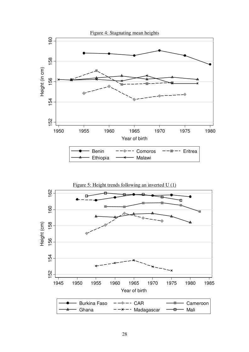
The development of heights stands in striking contrast to the good state in the
cross-section. For a number of countries either a downward or no clear trend can be
observed (Figure 3, Figure 4). Heights decreased at about one and a half centimetre in
Chad, Guinea, Namibia, and Zimbabwe. In Mozambique and Niger, the younger
cohorts attained a stature one centimetre smaller than the generation before. In Benin,
Comoros, Ethiopia, and Malawi, mean heights are nearly constant throughout the
entire period. For another group of countries, nutritional status followed an inverted U
indicating no sustained progress in health and nutritional conditions (Figure 5, Figure
6). Improvements mainly came to a halt in the birth cohorts of 1960s with mean
heights subsequently moving down to the level of the 1950 birth cohorts. Only in
Burkina Faso, CAR, Nigeria, and Togo a height advantage over the past still existed.
There are only a few sub-Saharan African countries showing a clear upward trend in
nutritional status (Figure 7). Kenyan women born in 1975 became two centimetres
taller than their counterparts born two decades before. In Cote d’Ivoire, the upward
trend is weak although very continuously. Tanzania and Senegal achieved impressive
gains in height of one centimetre per decade. However, growth came to a halt in the
1960s and the mean height of subsequent birth cohorts declined so that these countries
are more likely to follow the inverted U experience of the great bulk of African
countries.
We conclude that although many African countries made steps forward in the
second half of the 20th century, eventually almost the entire Southwest and Southeast
of the African continent went to a nutritional or health crisis. With the poor
development, the sub-Saharan region appears as an important exception from the
12
worldwide trend of upward-sloping heights indicating that the second half of the 20th
century cannot be treated as a period, in which progress in essential human needs took
place almost naturally.
The height series broadly follow the path of economic development. Sub-
Saharan African economies did well in the 1950s and 1960s. In the 1970s,
performances varied but in general, economic growth decelerated. In the 1980s, most
African countries experienced a severe and protracted economic crisis with
predominantly negative growth rates in per capita income. From this rough
description, it appears that the decline in nutritional status precedes the recession by
about one decade. Before going into the relationship between nutritional status and
economic growth, we clarify the modelling of the time structure of the cohorts’ mean
adult height on the one hand and environmental conditions on the other hand.
5. Modelling the time structure
We examine the changes in nutritional status from cohort to cohort applying a
birth cohort analysis. The dependent variable is the difference in mean height of
adjacent birth cohorts
(1) 1−−=∆ ttt yyy
Where y is mean height and t=1, 2, ..., 6 denotes the age groups 45-49, 40-44, ..., 20-
24 for a given country.5
5 Note that t can comprise different birth periods depending upon when the DHS-surveys took place. For instance, the age group 35-39 in the Ghana 2003 survey was born 1963-68, while the same age group in the Madagascar 1997 survey implies the birth years 1957-62.
13
For a regression analysis, it is important that the explanatory variables describe
the changes in conditions, under which the cohorts grew up. A straightforward
approach is to take the average from annual values covering the complete span of the
cohort’s birth years. Then, analogous to (1), we can take first order differences or
growth rates:
(2) 1−−=∆ ttt xxx
It is a common assumption that environmental conditions during the first years of life
determine final adult height while conditions at later ages are negligible (Baten, 2000;
Martorell and Habicht, 1986). The equation that reflects this assumption is
(3) uxytk
K
k kt +∆+=∆ � = ,10 ββ
However, adult height is a result of increases in stature from birth to maturity
and a lower adult height might have been caused by insults during childhood or
adolescence. Modelling the entire growth span is preferable. Brinkman et al. (1988)
assumed that the influence of environmental circumstances at a given age is
proportional to the share of growth typically accomplished at that age. They proposed
to use aggregated variables, where the annual values are weighted according to typical
Yearly Age and Sex Specific Increases in Stature (YASSIS). The problem with this
approach, however, is that it is uncertain whether a determinant indeed influences
bodily growth at all ages. Weighting the determinants dilutes the variance of the
explanatory variables. For instance, for a number of European countries Baten (2000)
found that real wages during the cohort’s first three years of life have the highest
explanatory power on final height, while the weighting scheme reduces the
explanatory power.
14
Our approach is based on the following consideration. If a changing
environment affects bodily growth at a particular age so that it influences final adult
height, a regression should be able to reveal this systematic impact (Figure 8). We
simply have to include those environmental changes after birth into the regression.
Technically, the explanatory variables are shifted temporally ahead.6 The general
form of the regression equation is
(4) uxxyZ
z mmtzmtztk
K
k tkt +∆+∆+=∆ � �� = = ++= 1
3
0,,,1 ,0 βββ
with K explanatory variables, which cover the cohorts’ birth period only, and Z
explanatory variables, for which we assume that they influence final adult height from
t to t+3. The regression coefficients �z,t+1, �z,t+2, and �z,t+3 roughly correspond to the
impact of environmental conditions during the first ( 1, +∆ tzx ), second ( 2, +∆ tzx ), and
third ( 3, +∆ tzx ) 5-year birth period respectively. Precise insights into the temporal
pattern are not feasible, as the cohorts cover 5-year age groups; uneven und
superjacent influences within the cohorts become smoothed and are expressed as an
average.
6. Determinants of the temporal variation in heights
In this section, we discuss factors, which might explain the poor development in
nutritional status. An important underlying determinant is economic growth. The
World Bank (1986) propagated that income is the binding constraint for an adequate
nutritional intake. There are many impoverished households in SSA spending a
6 It is also possible to shift the dependent variable temporally ahead and keeping the time structure of the explanatory variables unchanged, e.g. shifting the cohort’s mean height by one period would give
15
considerable fraction of their income on food. With income elasticities being high at
low levels of income, a rise in income would translate into higher food consumption.
Similarly, poor health is largely a result of poverty. The African climate, for instance,
is often blamed for the harsh disease environment though investments in public health
care can help to prevent or cure the diseases. It is due to poverty that medical
personnel, clinics, drugs and equipment, access to clean water and sanitation are
lacking. Overall, we would expect a positive impact of economic growth, especially
since idiosyncrasies like the specialization in livestock farming or climate related
exposure to diseases do hardly play a role for the temporal variation in height.
The income-height nexus can also be seen from a different perspective. In
African economies, work often relies on physical strength and endurance and,
therefore, on nutrition and health of the workers. Labour productivity provides the
link for a causality running from heights to income (Leibenstein, 1957; Strauss and
Thomas, 1998). In our analysis, endogeneity can arise from two sources. Firstly,
nutrition in the cohorts’ early years of life can positively correlate with nutrition and
health of the adult labour force (Fogel, 1994). If a better nourished and healthier
labour force is more productive, output increases. In this case, economic growth is
endogenous and the OLS coefficient would overestimate the actual influence of GDP/
c on nutritional status. Secondly, similar arguments apply, when the cohorts
themselves enter the labour force. Their own nutritional and health status gives rise to
the productivity link, even more so if nutritional status of women correlates with men
of the same age group.
We follow an instrumental variable approach to address the endogeneity of
GDP/ c. The empirical growth literature provides several candidates of valid IVs:
us the impact of the environment during late childhood.
16
From a neoclassical production function, it follows that output is a function of capital
and labour, so that the investment rate and growth in the labour force may predict
economic growth. An important variable in the African context is the black market
exchange rate premium, which is associated with distorting market practices and
reduced economic growth (Barro and Lee, 1994). The time, when the cohorts
themselves enter the labour force, may occur in t+3 at the earliest. We keep our set of
IVs but adjust the time structure accordingly.
GDP/ c is not the only potential determinant of nutrition and health. In order to
estimate a comprehensive regression model, we add several other variables to our
explanatory model. National food availability is one parameter for adequate dietary
intakes. The kind of food differs between the countries, e.g. in Zambia the staple food
is maize, and it is rice in Madagascar and sorghum and millet in Chad. With
expressing the food supply by the nutritional value, in calories or proteins, the overall
food situation becomes comparable. We include protein supply stressing the quality
aspect to a higher degree.7 Especially high quality food like meat, fish, eggs, and milk
contain large amounts of proteins. Milk is often fed to infants. Moreover, protein-rich
food has further important nutrients like calcium, iron and phosphorus, all of which
are important inputs for muscle and bone formation and therefore favour bodily
growth in particular.
A population’s nutritional status is not only determined by food availability but
also by nutritional needs. In particular, diseases inhibit the absorption of nutrients in
food and put a strain on children's energy. Unfortunately, reliable data on health
inputs are in scarce supply. Following Schneider (1996) und Weir (1993) we use the
7 In fact, growth rates of calorie and protein supply are highly correlated (R2: 0.80). In the cross-section, however, the correlation is rather weak, and here results point to proteins as the more powerful predictor of mean height (Moradi, 2005).
17
infant mortality rate as a proxy for the epidemiological environment. A drawback of
this proxy variable is that it might be determined simultaneously with nutritional
status.
Increases in family income need not necessarily translate into more resources
available to children. It is important to consider changes in intrahousehold allocation,
which we proxy with total fertility rate. Fertility is a choice between the quantity and
quality of children (Becker, 1960). Parents with fewer children have chosen to invest
more in quality, and as such in nutrition and health of their children. Therefore, an
decreasing fertility rate should be associated with a rise in mean height (Weir, 1993).
A variable, which let us directly observe investments into children, is the education
the cohorts attained. Education also serves as a proxy for the provision of public
goods other than schooling, so that we would expect a positive impact on nutritional
status.
In SSA, the great majority of people is living from agriculture. Rain fed
cropping systems are predominant which makes rainfall an essential input in
agriculture (Benson and Clay, 2000). Especially subsistence farmers, small tenants
and landholders, and pastoralists rely on rainfalls. A shortfall in rain causes their
endowment of food and income to fall while food prices simultaneously rise. Thus,
their food security depends on the quality of each rainy season. Large landowners and
city dwellers, in contrast, are less vulnerable to climatic shocks. Factors shielding the
cities range from a better accessibility to food policies biased in favour of urban areas.
Consequently, droughts have distributional effects that are not accounted by economic
growth.
Extreme droughts triggering devastating famines occurred in 1968-1973 in
Ethiopia and the Sahel (Dinar and Keck, 2000). In 1974-1985, a second wave of
18
droughts followed; from the 28 countries in our sample, 21 countries had more than
two consecutive drought years. In addition to short-term shocks, the Sahel countries
experienced a systematic decrease in rainfall; precipitation in the period 1961-90 was
10-20% lower than the three decades before (Hulme, 1992). Overall, we expect that
droughts as well as less severe deviations from normal rains affect nutritional status
negatively.8
Civil wars are another all too frequent tragedy in SSA with detrimental effects
on nutrition and health. Farmers are prevented from timely sowing and harvesting or,
fleeing the war, they completely abandon their fields; blocked roads and partitioning
disrupt the allocation of goods and foods. The epidemiological environment is also
likely to deteriorate. The destruction of health facilities and cuts in their capacities let
break down basic health care delivery like vaccinations or prenatal care; other
services important for hygiene like water pumps can often not be maintained. Refugee
movements and poor hygiene are fertile grounds for the spread of infectious diseases
(Kalipeni and Oppong, 1998). During conflicts, military expenditures increase
considerably crowding out health care investments. Thus, civil wars affect the public
health system in a time of increased need. The adverse effects make it likely that
cohorts born in times of civil war suffer from deteriorating nutritional status. In our
sample, the most war-torn countries are Chad, Ethiopia, Mozambique, Nigeria,
Uganda, and Zimbabwe.
We finally include urbanization. Indicating a transition from a traditional to a
modern and industrialised society, the process of urbanisation is associated with an
increased complexity in the value added chain (Tiffen, 2003). Therefore, urbanization
8 It would be ideal to follow the conceptualisation of agricultural droughts, which refer to situations in which soil moisture is insufficient to meet the needs of the plants (Glantz, 1987). For example, apart from total rainfall, the right distribution during the different stages in the crop’s development is equally
19
can complement GDP/ c, e.g. if primary commodity booms inflate national income
without a broad diffusion of benefits like in Gabon, Namibia, Nigeria, or Zambia.
Moreover, there is a large urban-rural divide in living standards. Urban areas provide
better housing, health services, employment opportunities, access to public goods like
water and sanitation services, and so on. On average, city dweller enjoy an height
advantage (Loaiza, 1997). Urbanization could simply mean an increasing share of
population, which benefits from the amenities.
7. Results
The regression analysis reveals very interesting insights (Table 3). In contrast to
the lack of correlation between GDP/ c and mean height in the cross section, we find
that economic growth does affect the development of mean heights significantly
positively. The time structure of the influence is very interesting. Besides a positive
effect of economic growth in early years of life (in t), we additionally find a positive
effect in t+3, which roughly corresponds to the time of puberty (OLS (2), Table 3). It
is widely acknowledged that bodily growth is very sensitive to conditions during early
years of life. After weaning, toddlers have quantitatively and qualitatively high energy
needs and they are highly vulnerable to infections due to unhygienic conditions or
contaminated food (Martorell and Habicht, 1986). Since a large share of total height is
acquired in the first three years of life, growth retardation in early years of life
translates into a permanent loss of stature, especially when conditions do not improve
dramatically so that catch-up growth is negligible. It is also known that undernutrition
shapes bodily growth at puberty delaying the adolescent growth spurt, slowing down
important. Though the concept of agricultural droughts does better describe conditions eventually
20
bodily growth and lengthen the growth span (Bogin, 1988). Some scholars believe
that the prolonged growth phase balances out the lower growth velocity (Kulin et al.,
1982). However, our results suggest that conditions at puberty did contribute to the
deficit in final adult height of African women.
Acknowledging the effect at puberty is important to avoid misinterpretations. In
many African countries, the development of mean height followed an inverted U with
the trend reversal often occurring in cohorts born in the mid-1960s (Figure 5, Figure
6). From these trends, we cannot infer that environmental conditions started to
deteriorate in the 1960s. The significant coefficient of economic growth in t+3
demonstrates that instead, the crisis of the late 1970s and 1980s and its influence on
body growth at puberty must be partly considered responsible for the falling mean
adult heights of the mid-1960s birth cohorts. It is noteworthy, that the severe
economic crisis in the 1980s may have given raise to the influence at puberty. When
we restrict the sample on cohorts born before 1965, we find the impact in t+3 reduced
(though the effect in t+2 becomes stronger).
The impact of economic growth is substantial. Growth in GDP/ c between the 5-
year age cohorts averages 4% and varies with a standard deviation of 12.4 between -
27% and 36% (OLS (1) and (2), Table 3).9 Hence, a difference in economic growth in
the order of one standard deviation would change mean adult height of the cohort,
which is in their infanthood (the impact in t), as well as the cohort, which is in the age
of puberty (the impact in t+3), by 0.1 cm.
In the first two regressions, unavailable data on protein supply and urbanization
restrict our analysis to cohorts born 1963-84. When excluding these variables, the
leading to lower yields, no data exists for our purposes. 9 The figures refer to �GDP/ c t. �GDP/ c t+3 , which covers the 1980s and even 1990s, averages -4% and varies with a standard deviation of 11.8 between -46% and 23%.
21
sample increases in size and covers cohorts born in the 1950s (OLS (3) and (4), Table
3). The impact of economic growth is increasing in significance. Moreover, we can
find the positive influence in t+3 crossed over to t+2. We also ran a country fixed
effects regression in order to control for country-specific, deterministic time trends in
height (FE (5), Table 3). Under this specification, the estimated impact of income
almost doubles. Though fixed effects are not significant at conventional levels (p-
value: 0.13), they indicate that the experience of at least some countries differs. This
is the case for Niger and CAR, where the development of mean height was
consistently better than expected. In Namibia and Zimbabwe, in contrast, mean
heights were ceteris-paribus decreasing by half a centimetre per 5-year-cohort. One
may wonder whether the social and economic discrimination of the black majority in
both countries might be the reason that nutrition and health deteriorated despite of
substantial economic growth (Figure 3).10
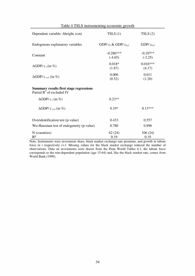
The link between nutrition and labour productivity makes income growth
possibly endogenous. In this case, OLS estimates would be upwardly biased. We
therefore instrument for economic growth in both, t and t+3. The size of the TSLS
coefficient for income growth in t ranges between the OLS and FE estimator (TSLS
(1), Table 4). Moreover, the influence is significantly positive. The effect in t+3 is
also positive, but slightly lower and insignificant. The reason for this result is that,
surprisingly, our IVs are less powerful for economic growth in t+3, i.e. the IVs do not
have a highly significant impact on economic growth (p-value: 0.06), and the lower
efficiency of TSLS translates into large standard errors. Accepting the exogeneity of
economic growth in t and running the TSLS again with economic growth endogenous
10 Note, that the slope coefficient of economic growth is assumed to be equal for all countries. When testing for a structural break in the height-economic growth relationship for those countries, the coefficients of economic development turned out to be very similar indicating that the concern is indeed country-specific differences in the development of mean height.
22
in t+3 only increases the sample size (TSLS (2), Table 4). Though the IVs
comfortably pass the relevance test (p-value: 0.00), significance does not increase to
conventional levels. Nevertheless, the size of the TSLS coefficient is very similar to
the OLS one. This confirms the Wu-Hausman test indicating that we cannot reject the
null of exogeneity of economic growth.
There are factors, which can dwarf the case of endogeneity at the macro level.
Nutrition of labourers and children need not correlate very strongly. Given the
nutrition-productivity link, we would expect a utility maximising household to treat
its members unequally (Behrman, 1997; Dasgupta, 1997). In fact, the consumption of
household members, whose labour contributes to the household’s income, might be
rather inelastic. Furthermore, one may doubt, whether total value added, to which a
single 5-year age group of juvenile age contributes (in t+3), is significant enough that
increased labour productivity caused by a taller stature measurably influences
economic growth.
The importance of economic development is overwhelming.11 When controlling
for other determinants only the proxy variables of nutrition and health are significant
predictors of height. Food supply in form of proteins influences nutritional status
significantly positively, which is in line with studies of child undernutrition
(Brinkman and Drukker, 1998; Smith and Haddad, 2000). A ten percent rise in protein
supply over a 5-year period would increase mean heights by about 0.2 cm. Like
economic growth, food supply is fitting the overall height pattern particularly well. In
the late 1960s, growth rates in per capita food availability tended to decrease and
African countries became more homogeneous in this respect. Infant mortality rate also
11 One can argue that economic growth is an underlying determinant, which influences immediate determinants like health environment and food supply. Given this causal framework, the determinants should be treated rather separately. Unsurprisingly, including them into a single explanatory model reduces the effect of economic growth in t.
23
has the expected negative sign, so that declining infant mortality rates were associated
with increasing mean heights of African women. Taking the infant mortality rate as
health indicator, progress in health only slightly slowed down in the 1970s, and
therefore, health cannot explain the overall trend in nutritional status.
The other variables do not add much explanatory power (OLS (2) and OLS (4),
Table 3). The education the cohorts attained is insignificant. Micro studies of
undernutrition, in contrast, regularly found a positive effect, notably of the mothers’
education. Her education increases the likelihood of good childcare practices.
Accurately modelling this effect at the macro level is unfeasible. However, we would
also argue that education serves as an indicator of social status, which let micro
studies overestimate the true influence of education. The civil war variable is also
insignificant. Though without doubt, ordinary people always suffer in conflicts, the
effects appear to be sufficiently accounted for by economic growth. On average, civil
wars are associated with a 10% fall in GDP/ c suggesting that nutritional status
decreases in the course of civil wars. Finally, fertility and urbanization cannot explain
the development of mean heights in SSA and though rainfall has the expected positive
impact (OLS (3), Table 3), it is not very robust.
8. Summary
Advocates of an optimistic view of African development emphasized
achievements in soft indicators like education, child mortality, and life expectancy,
which stand in some contrast to the poor economic performance of SSA. In this paper,
we focused on another dimension of the quality of life. We studied mean heights,
which reflect nutrition and health the populations have faced during bodily growth.
24
Using heights of more than 200,000 women from 28 sub-Saharan African countries,
we found that nutritional status was in a good state in the 1960s. However, the
development of heights indicates a deterioration of nutritional status. In a number of
countries, mean heights stagnated or decreased and even though several African
countries made some improvements, eventually the entire Southwest and Southeast of
the African continent went to a nutritional crisis. Overall, sub-Saharan Africa
represents an important exception to the trend of upward-sloping heights found in
almost all other regions of the world in the 20th century.
In a regression analysis, we tested the explanatory power of the economic
development and several other determinants on temporal height variations. The results
indicate that economic growth was a powerful factor influencing the physical growth
process at two distinct periods: during infanthood as well as adolescence. Income
shocks at both times had a lasting effect on final adult height. The effect at puberty
suggests that the severe economic crisis of the late 1970s and 1980s played a role for
the trend reversal occurring in cohorts born in the mid-1960s. We also took into
account the endogeneity of income, plausible via the nutrition-productivity link, but
did not find evidence of endogeneity. The results have also implications for one of
today’s most pressing problems. In the fight against undernutrition, a promising
weapon is bringing African countries back to the path of economic growth they left in
the 1970s.
25
Figure 1: Height trends of the genders in Cote d’Ivoire and Ghana
Note: The data is drawn from the Living Standard Measurement Study surveys GLSS 1988/89 and CILSS 1985/86/87/88 (World Bank). About 40% of the individuals in the CILSS and 60% in the GLSS survey were remeasured in a second round. Inconsistencies between the first and second rounds (sex, age > 5 years, height > 10 cm) as well as extreme outliers were excluded; remaining minor deviations were averaged. In total, the Ivorian (Ghanaian) mean heights are based on 9484 (8138) native born individuals between 20 and 49 years of age.
Note: GDP/c figures are from Penn World Tables 6.1 (Heston et al., 2002). US GDP/c (PPP) in 1820, 1870, and 1913 was approximately 1360, 2650, and 5740 (Maddison, 2001).
27
Figure 3: Decreasing mean heights
154
156
158
160
162
164
Hei
ght (
cm)
1945 1950 1955 1960 1965 1970 1975 1980
Year of birth
Chad Guinea MozambiqueNamibia Niger Zimbabwe
Note: Birth cohorts are based on 5-year age groups (45-49, 40-44, ..., 20-24). The year of birth corresponds to the cohort mean and was assigned to the nearest 2.5-year segment. Cohorts with less than 100 individuals were excluded. All-women surveys, which are representative of the total female population, are in solid lines.
28
Figure 4: Stagnating mean heights
152
154
156
158
160
Hei
ght (
in c
m)
1950 1955 1960 1965 1970 1975 1980
Year of birth
Benin Comoros EritreaEthiopia Malawi
Figure 5: Height trends following an inverted U (1)
152
154
156
158
160
162
Hei
ght (
cm)
1945 1950 1955 1960 1965 1970 1975 1980 1985
Year of birth
Burkina Faso CAR CameroonGhana Madagascar Mali
29
Figure 6: Height trends following an inverted U (2)
156
158
160
162
Hei
ght (
cm)
1945 1950 1955 1960 1965 1970 1975 1980
Year of birth
Mauritania Nigeria RwandaTogo Uganda Zambia
Figure 7: Increasing mean heights
154
156
158
160
162
Hei
ght (
cm)
1945 1950 1955 1960 1965 1970 1975 1980
Year of birth
Cote d’Ivoire Gabon KenyaSenegal Tanzania
30
Figure 8 Modelling the entire growth period with leaded explanatory variables
Period of growth (five-year periods)
tx∆ 1+∆ tx 2+∆ tx 3+∆ tx
�yt
t t+1 t+2 t+3
Final adult height Bodily growth in
Economic development
31
Table 1 Anthropometric data in the DHS-surveys
Country Date of survey Coverage
(M=Mothers, AW=all women)
Number of women (Age group 20-49)
Benin 1996 & 2001 M & AW 2400 & 4957
Burkina Faso 1992/93 & 1998/99 & 2003 M & M & AW 3459 & 3569 &
9547 Cameroon 1998 & 2004 M & AW 1609 & 3890 CAR 1994/95 M 2050 Chad 1996/97 & 2004 M & M 3940 & 3193 Comoros 1996 M 835 Cote d’Ivoire 1994 & 1998/99 M & AW 3017 & 2221 Eritrea 1995 M 1836 Ethiopia 2000 AW 11656 Gabon 2000 M 2359
Ghana 1993 & 1998 & 2003 M & M & AW 1785 & 2216 &
4374 Guinea 1999 M 3401
Kenya 1993 & 1998 & 2003 M & M & AW 3425 & 3378 &
6010 Madagascar 1997 M 2580 Malawi 1992 & 2000 M & AW 2495 & 10152 Mali 1995/96 & 2001 M & AW 4438 & 9833 Mauritania 2000 AW 5910 Mozambique 1997 & 2003 M & AW 3158 & 9253 Namibia 1992 M 2381 Niger 1992 & 1998 M & M 3569 & 3466 Nigeria 2004 AW 5737 Rwanda 2000 AW 7544 Senegal 1992/93 M 3178 Tanzania 1992 & 1996 M & M 4711 & 3959 Togo 1998 M 3470 Uganda 1995 & 2000/01 M & AW 3401 & 5118
Zambia 1992 & 1996 & 2001/02 M & M & AW 3386 & 4084 &
5762 Zimbabwe 1994 & 1999 M & AW 1948 & 4219 Total: 28 countries 1992 - 2004 31 M & 16 AW 198879
Note: Based on surveys that were available by March 2006. We excluded the age group 15-19, because some of the individuals are still growing at this age. We also excluded height measurements departing from the birth cohort mean by more than three standard deviations.
32
Table 2 Height difference between women and mothers
Height difference (in cm) women - mothers Age group
Mean Standard deviation
Share of mothers (%)
45-49 0.074 0.587 22.1
40-44 -0.064 0.450 45.3
35-39 0.012 0.283 64.5
30-34 0.069 0.161 75.2
25-29 0.052 0.159 78.4
20-24 0.144 0.216 66.5
Total (N=96) 0.048 (1.359) 0.344 58.7
Note: Mothers are defined as women who had given at least one birth in the 59 months prior to the date of interview. Based on Benin, Burkina Faso, Cameroon, Cote d’Ivoire, Ethiopia, Ghana, Kenya, Malawi, Mali, Mauritania, Mozambique, Rwanda, Uganda, Zambia, and Zimbabwe (N=16 per age group); t-value of the null hypothesis that the height of women and mothers are equal in parentheses.
33
Table 3: OLS-Determinants of temporal variation in heights Dependent variable: �height (cm) OLS (1) OLS (2) OLS (3) OLS (4) FE (5)
Note: Birth cohorts with less than 100 individuals were excluded. t statistics in parentheses; coefficients significant to the 10%/ 5%/ 1% level are marked with */**/***. The data for the explanatory variables were taken from a couple of sources. The figures on protein supply, available from 1961 onwards and referring to food supply available for human consumption, are derived from the FAO Food Balance Sheets (FAOSTAT). The gender specific infant mortality rate and the total fertility rate are drawn from UN Population Division (2003). The rainfall data stems from Mitchell et al. (2004), version 1.1, and are calculated for the countries’ territory. From the Correlates of War Project, we derived the start and duration of wars of decolonization as well as civil wars (Sarkees, 2000). A threshold of 1000 battle related deaths per year guarantees that we include major wars, which presumably affected a large part of the population. Due to averaging a dummy, the civil war variable in Table 3 describes the relative length of the birth period [0-1], during which a civil war took place. Thus, a value of zero indicates that peace prevailed during the full length of the cohort’s birth period, while a value of one indicates that a civil war took place in every year of the birth period. The share of urban population was taken from World Bank (1999). Finally, the GDP figures are from Maddison (2001), who provides data from 1950 onwards; missing values for Burkina Faso, Ethiopia, Guinea, and Malawi were interpolated with data from the Penn World Tables 6.1 (Heston et al., 2002).
Summary results first stage regressions Partial R2 of excluded IV
�GDP/ c t (in %) 0.23**
�GDP/ c t+3 (in %) 0.19* 0.13***
Overidentification test (p-value) 0.433 0.557
Wu-Hausman test of endogeneity (p-value) 0.780 0.896
N (countries) 62 (24) 106 (24) R² 0.19 0.19
Note: Instruments were investment share, black market exchange rate premium, and growth in labour force in t respectively t+3. Missing values for the black market exchange reduced the number of observations. Data on investments were drawn from the Penn World Tables 6.1, the labour force corresponds to the non-dependent population (age 15-64) and, like the black market rate, comes from World Bank (1999).
35
References Barro, R. J. and J.-W. Lee (1994). Sources of Economic Growth. Carnegie-Rochester Conference
Series on Public Policy 40: 1-46. Baten, J. (2000). Height and Real Wages: An International Comparison. Jahrbuch für
Wirtschaftsgeschichte 2000-1: 17-32. Baten, J. (2003). Anthropometrics, Consumption, and Leisure: The Standard of Living. Germany: A
New Social and Economic History, Vol. 3: Since 1800. S. Ogilvie and R. Overy. London: Edward Arnold.
Baten, J. and J. E. Murray (2000). Heights of Men and Women in 19th Century Bavaria: Economic,
Nutritional, and Disease Influences. Explorations in Economic History 37(4): 351-369. Becker, G. S. (1960). An Economic Analysis of Fertility. Demographic and Economic Change in
Developed Countries. Universities--National Bureau Committee for Economic Research. Princeton: Princeton University Press: 209-231.
Behrman, J. R. (1997). Intrahousehold Distribution and the Family. Handbook of Population and
Family Economics. M. R. Rosenzweig and O. Stark. Amsterdam: North Holland Press: 125-187.
Benson, C. and E. Clay (2000). The Economic Dimensions of Drought in Sub-Saharan Africa.
Drought: A Global Assessment. D. A. Wilhite. London: Routledge. 1: 287-310. Bogin, B. (1988). Patterns of Human Growth. Cambridge: Cambridge University Press. Brinkman, H.-J. and J. W. Drukker (1998). Does the Early-Economic-Growth-Puzzle Apply to
Contemporary Developing Countries? The Biological Standard of Living in Comparative Perspective. J. Komlos and J. Baten. Stuttgart: Franz Steiner Verlag: 55-89.
Brinkman, H.-J., J. W. Drukker and B. Slot (1988). Height and Income: A New Method for the
Estimation of Historical National Income Series. Explorations in Economic History 25(3): 227-264.
Cline, M. G., K. E. Meredith, J. T. Boyer and B. Burrows (1989). Decline of Height with Age in Adults
in a General Population Sample: Estimating Maximum Height and Distinguishing Birth Cohort Effects from Actual Height Loss of Stature with Aging. Human Biology 61(3): 415-425.
Dasgupta, P. (1997). Nutritional Status, the Capacity for Work, and Poverty Traps. Journal of
Econometrics 77(1): 5-37. Dinar, A. and A. Keck (2000). Water Supply Variability and Drought Impact and Mitigation in Sub-
Saharan Africa. Drought: A Global Assessment. D. A. Wilhite. London: Routledge. 2: 129-148.
Eveleth, P. B. and J. M. Tanner (1990). Worldwide Variation in Human Growth. Cambridge:
Cambridge University Press. Ewbank, D. C. (1981). Age Misreporting and Age-Selective Underenumeration: Sources, Patterns, and
Consequences for Demographic Analysis. Committee on Population and Demography Report No. 4. Washington, D.C., National Academy Press.
FAOSTAT. FAO Statistical Data Bases. from http://apps.fao.org/. Fiawoo, D. K. (1979). Physical Growth and the School Environment: A West African Example.
Physiological and Morphological Adaptation and Evolution. W. A. Stini. The Hague: Mouton: 301-314.
36
Fogel, R. W. (1994). Economic Growth, Population Theory, and Physiology: The Bearing of Long-
Term Processes on the Making of Economic Policy. American Economic Review 84(3): 369-394.
Glantz, M. H. (1987). Drought and Hunger in Africa: Denying Famine a Future. Cambridge:
Cambridge University Press. Habicht, J.-P., C. Yarbrough, R. Martorell, R. M. Malina and R. E. Klein (1974). Height and Weight
Standards for Preschool Children: How Relevant Are Ethnic Differences? Lancet 303 (7858): 611-615.
Heston, A., R. Summers and B. Aten (2002). Penn World Table Version 6.1, Center for International
Comparisons at the University of Pennsylvania (CICUP). Hill, A. (1992). Trends in Childhood Mortality in Sub-Saharan Mainland Africa. Mortality and Society
in Sub-Saharan Africa. E. van de Walle, G. Pison and M. Sala-Diakanda. Oxford: Clarendon Press: 10-31.
Hulme, M. (1992). Rainfall Changes in Africa: 1931-60 to 1961-90. International Journal of
Climatology 12: 685-699. Kalipeni, E. and J. Oppong (1998). The Refugee Crisis in Africa and Implications for Health and
Disease: A Political Ecology Approach. Social Science & Medicine 46(12): 1637-1653. Klasen, S. (1996). Nutrition, Health, and Mortality in Sub Saharan Africa: Is There a Gender Bias?
Journal of Development Studies 32(6): 913-932. Komlos, J. (1999). On the Biological Standard of Living in Russia and the Soviet Union. Slavic Review
58(1): 71-79. Kuczmarski, R. J., C. L. Ogden, S. S. Guo, L. M. Grummer-Strawn, K. M. Flegal, Z. Mei, R. Wie, L.
R. Curtin, A. F. Roche and C. L. Johnson (2002). 2000 CDC Growth Charts for the United States: Methods and Development. Vital and Health Statistics 11(246): 1-190.
Kulin, H. E., N. Bwibo, D. Mutie and S. J. Santner (1982). The Effect of Chronic Childhood
Malnutrition on Pubertal Growth and Development. American Journal of Clinical Nutrition 36(3): 527-536.
Leibenstein, H. (1957). Economic Backwardness and Economic Growth: Studies in the Theory of
Economic Development. New York: Wiley. Loaiza, E. (1997). Maternal Nutritional Status. DHS Comparative Studies No. 24. Calverton, Maryland,
Macro International Inc. Macro. Demographic and Health Surveys. Retrieved March, 2006, from http://www.measuredhs.com. Maddison, A. (2001). The World Economy: A Millennial Perspective. Paris: Development Centre of the
Organisation for Economic Co-operation and Development. Martorell, R. and J.-P. Habicht (1986). Growth in Early Childhood in Developing Countries. Human
Growth: A Comprehensive Treatise. F. Falkner and J. M. Tanner. New York: Plenum. 3: 241-262.
Meisel, A. and M. Vega (2005). A Tropical Success Story: A Century of Improvements in the
Biological Standard of Living, Colombia 1910-2002. Fifth World Cliometrics Congress, Venice, Italy.
Mitchell, T. D., T. R. Carter, P. D. Jones, M. Hulme and M. New (2004). A Comprehensive Set of
High-Resolution Grids of Monthly Climate for Europe and the Globe: The Observed Record
37
(1901-2000) and 16 Scenarios (2001-2100). Tyndall Centre Working Paper No. 55. Tyndall Centre for Climatic Change Research.
Moradi, A. (2005). Ernaehrung, wirtschaftliche Entwicklung und Buergerkriege in Afrika suedlich der
Sahara (1950-2000). Faculty of Economics, University of Tuebingen. PhD thesis. Moradi, A. and J. Baten (2005). Inequality in Sub-Saharan Africa: New Data and New Insights from
Anthropometric Estimates. World Development 33(8): 1233-65. Moradi, A. and A. M. Guntupalli (forthcoming). What Does Gender Dimorphism in Stature Tell Us
About Discrimination in Rural India, 1930-1975? Gender Bias: Health, Nutrition and Work. M. Pal, P. Bharati, B. Ghosh and T. S. Vasulu. New Dehli: Oxford University Press.
Oxley, D. (2004). Living Standards of Women in Prefamine Ireland. Social Science History 28(2): 271-
295. Sarkees, M. R. (2000). The Correlates of War Data on War: An Update to 1997. Conflict Management
and Peace Science 18(1): 123-144. Schneider, R. (1996). Historical Note on Height and Parental Consumption Decisions. Economics
Letters 50(2): 279-283. Sender, J. (1999). Africa’s Economic Performance: Limitations of the Current Consensus. Journal of
Economic Perspectives 13(3): 89-114. Smith, L. C. and L. Haddad (2000). Explaining Child Malnutrition in Developing Countries: A Cross-
Country Analysis. Washington, D.C.: International Food Policy Research Institute. Steckel, R. H. (1995). Stature and the Standard of Living. Journal of Economic Literature 33(4): 1903-
1940. Strauss, J. and D. Thomas (1998). Health, Nutrition, and Economic Development. Journal of Economic
Literature 36(2): 766-817. Tiffen, M. (2003). Transition in Sub-Saharan Africa: Agriculture, Urbanization and Income Growth.
World Development 31(8): 1343-1366. UN Population Division (2003). World Population Prospects: The 2002 Revision. New York: United
Nations. UNICEF (1996). The State of the World’s Children. New York: Oxford University Press. van Wieringen, J. C. (1972). Secular Changes of Growth: 1964-1966 Height and Weight Surveys in the
Netherlands in Historical Perspective: Review, Tables and Graphs. Leiden: Netherlands Institute for Preventive Medicine.
Weir, D. R. (1993). Parental Consumption Decisions and Child Health During the Early French
Fertility Decline, 1790-1914. Journal of Economic History 53(2): 259-274. WHO (1966). Malaria Eradication in 1965. WHO Chronicle 20: 286-300. WHO (1983). World Health Statistics Annual. Geneva: WHO. World Bank. Living Standard Measurement Study. Retrieved 2001, from
http://www.worldbank.org/lsms/. World Bank (1986). World Development Report. New York: Oxford University Press. World Bank (1999). 1998 World Development Indicators on CD-ROM. Washington, D.C.: World