NVF III Session 2 Statistics

NVF III Session 2Statistics

Presented by Ashley Isbel12 May, 2014

Slide 2 © PharmOut 2014

This Session

This session will cover

Statistics – what do we do well?

Statistics – what could we do better?

Statistics – what causes blank stares?


Statistics … there’s no escape!


Statistics

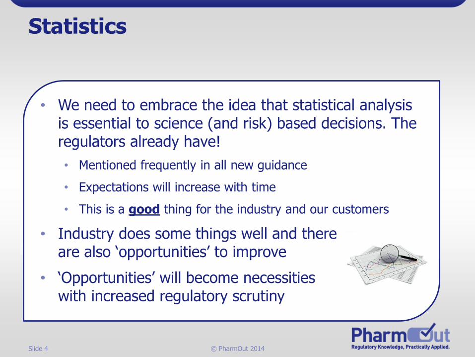
• We need to embrace the idea that statistical analysis is essential to science (and risk) based decisions. The regulators already have!

• Mentioned frequently in all new guidance

• Expectations will increase with time

• This is a good thing for the industry and our customers

• Industry does some things well and thereare also ‘opportunities’ to improve

• ‘Opportunities’ will become necessitieswith increased regulatory scrutiny


What do we do well?

• Statistics have found some common use in qualification and validation activities

• Some statistical tools that are generally used well:

• Process Capability - Cp & Cpk

• Run and control charting (with some caveats)

• Application of AQL (with some caveats)


Potential Capability (Cp and Cpk)

• Capability indices are ratios (no units) that compare the tolerance (width of the specification) to the process spread (variability of the process)

Fill weight

Histogram of Weight

Weight


Cpk in Qualification vs Validation

• Process capability is not applicable to everything requiring Q/V (mixing, heating, sterilisation, etc)

• used to assess capability with regard to:

• Assay, Yield

• Other analysed specification limits

• Fill volume/weight

• Capability studies in qualification generally should not include routine interventions or adjustments!

• Capability studies for process validation generally should include routine interventions and adjustments!


Process Capability

Benefits• Very easy to compare process to process, or trial to trial.

• Makes variability a key parameter of assessment.

• Provides quantitative assessment of capability.

• Practically easy to understand.

Weaknesses

• Not easily visual, ‘just a number’.

• Requires normally distributed data.

• Doesn’t easily detect deterioration in capability over time.


Run charts (time series)

Run charts are the simplest statistical representation for sequential data:

Will indicate trends: upward, downward, cycles, shift-based, product, process etc

Weight (g)

Order of data collected


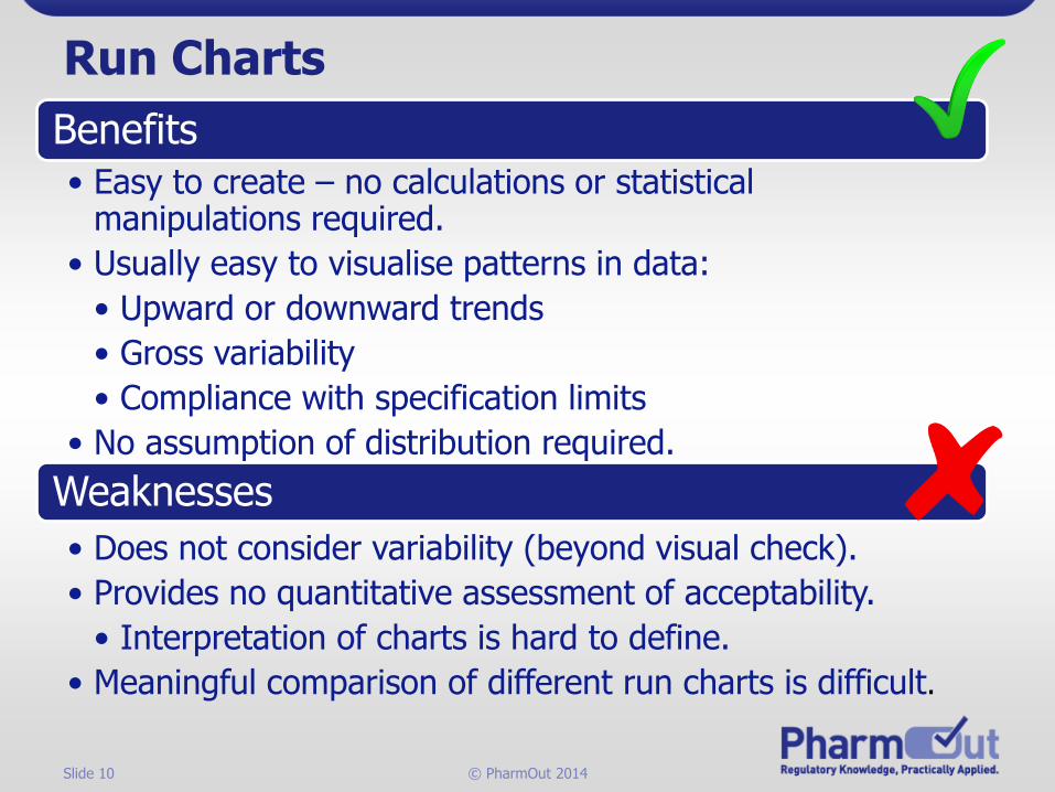
Run Charts

Benefits

• Easy to create – no calculations or statistical manipulations required.

• Usually easy to visualise patterns in data:

• Upward or downward trends

• Gross variability

• Compliance with specification limits

• No assumption of distribution required.

Weaknesses

• Does not consider variability (beyond visual check).

• Provides no quantitative assessment of acceptability.

• Interpretation of charts is hard to define.

• Meaningful comparison of different run charts is difficult.


Control Charts

Control Limits represent the normal amount of variation over time

Limits are calculated using the variation of our data and are often referred to as sigma limits (typically 3)

Weight (g)

Observation

Sample mean (x bar)

Upper Control Limit (UCL)

Lower Control Limit (LCL)

Control Chart of Weight


Control Charts

Control charts are simply run charts modified to determine control limits for processes. They can be used to:

Establish specification

limits

Confirm control is

within specification

limits

Assist with identifying

variability so that a process

can be modified


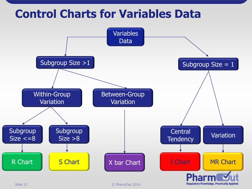
Control Charts for Variables Data

Variables Data

Subgroup Size >1

Between-Group Variation

Within-Group Variation

Subgroup Size >8

Subgroup Size <=8

X bar ChartR Chart S Chart

Subgroup Size = 1

Central Tendency

Variation

MR ChartI Chart


Sampling for Acceptance

Sampling for acceptance is the most common way of developing sampling plans in GMP.

What is the purposes of Acceptance Sampling?

• Provides criteria for and determines the acceptability level of incoming or outgoing materials.

• Acceptability level is commonly termed “Acceptable Quality Level” – the minimum level at which a lot is accepted.

• AQL is not a measure of quality. Acceptance sampling tells you very little about the quality of a lot. – it is just not robust enough.


Sampling for Acceptance

Acceptance sampling is an internationally accepted means of compromise between statistical confidence and economics:

• Rejecting good material (bad for manufacturer)

• Accepting bad material (bad for consumer)

Real, but small risks of:

• Vendor assurance

• In-process testing

• Process validation

• Environmental controls

• Personnel controls, etc.

GMP companies usually have a number of other mitigation strategies to

reduce these risks:


What could we do better?

• Some statistical tools are used in PV, but not with the same frequency, or aren’t as well understood.

• Some of these include:

• Sampling plans

• Assessment of statistical methodology

• Use of confidence intervals

• Understanding variation


Sampling Plans

• The sampling plan, including sampling points, number of samples, and the frequency of sampling for each unit operation and attribute. The number of samples should be adequate to provide sufficient statistical confidence of quality both within a batch and between batches. The confidence level selected can be based on risk analysis as it relates to the particular attribute under examination.

• AQL tables do not always fulfil all of these requirements

• To draw conclusions about a population, the sample must be random.

• Samples should be representative


Assessment of methodology

• Where statistical analysis of PV is performed, sometimes we see

• Entrenched methods, driven by guidelines and procedures

• Methods used ad-hoc, selected for a specific exercise

• Either way, assessment of the methodology is frequently lacking

• Assessment of the validity of the method

• Assessment of the suitability of the method


Testing for Validity - Normality

• Most basic statistical tools assume normal distribution

• In practice, no processes are exactly ‘normally’ distributed.

• Histograms provide a quick check to see if the distribution approximates normal distribution. If it does, it is usually acceptable to use the data as is.

• GMP results lend themselves to approximating normal distribution. But it is not always the case.


How to test for normality

Histogram Probability Plot

Hypothesis test


Histogram

Like a Bar Chart but can display numeric data:

Each bar represents the frequency of data values that occur in each interval

Weight (g)

Frequency


Hypothesis Tests

• When a hypothesis test is conducted, the results include a test statistic and a p-value.

• The p-value is used to determine whether we should reject or fail to reject the null hypothesis.

• The calculated p-value is compared against the selected α (Alpha) value (the acceptable statistical confidence for the test)


Confidence Intervals

• Normal distributions are defined by Mean and StDev -single values that approximate the true value of the population parameter

• It is highly unlikely that the sample mean and StDevwe obtain are exactly the same as the true population parameters

• To get a better sense of the true population values, we can use confidence intervals-a likely range of values for a population parameter (mean or StDev)


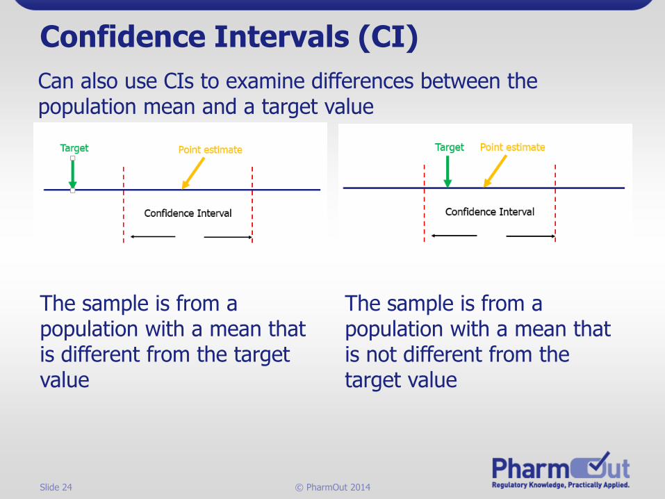
Confidence Intervals (CI)

Can also use CIs to examine differences between the population mean and a target value

The sample is from a population with a mean that is different from the target value

The sample is from a population with a mean that is not different from the target value


Confidence Intervals (CI)

• Always a chance that CI will not contain the true population mean.

• Must decide how sure we need to be that the CI contains the actual population parameter value-confidence level

• The higher the confidence level (i.e. 95%), the wider the confidence interval


Understanding Variability

• In any given GMP manufacturer:

• How many OOS values are documented each year?

• How many manufacturing deviations are investigated each year?

• How many lots are rejected each year?

• How many quality problems would go away if there were no variation?

• What if we could reduce variation



• What is Variability? a statistical term to describe the inherent variation of experimental data.

• Common cause variation is that which is created by the variability of all the inputs into a process.

• It is possible to predict, minimise and allow for common cause variation

• Special (or assignable) cause variation is that which is created by an unexpected circumstance.

• It is not possible to predict, although it may be possible to minimise and allow for.



• Common thoughts on variability:

• Old technology is responsible – new tech would solve the problem.

• Too many tests leads to higher variability.

• Variability exists because someone didn’t do their job correctly.

• Variability is an inherent fact of life and there isn’t anything we can do about it except to live with it. It’s cost of business.

• In reality, there are two types of variability – one we can eliminate (special cause) and one we can reduce (common cause).



“Special Cause” (or assignable cause) variation is the result of a single source.

• Use CAPA to solve it.

• Find variation Attribute cause eliminate cause.

“Common Cause” variation is the result of multiple small sources all contributing to the sum total.

• CAPA will not work for common cause.

• Culture or organisationalchange is required to address common cause variation.


What usually prompts blank looks?

• There are a few statistical tools and concepts that are potentially very useful in PV, but are poorly understand and highly underutilised

• We will look at two in a bit more detail:

• Analysis of Variance (ANOVA)

• Design of Experiments (DoE)


Analysis of Variance (ANOVA)

• ANOVA is a collection of statistical models used to analyse the differences between the means of different test subjects, and therefore the different procedures which produce the subjects

• ANOVA can consider 1 factor (1 way ANOVA) or multiple factors

• 1 and 2 way models are common. Consideration of higher numbers of factors is usually the domain of statisticians and often requires DoE assistance.


One-way ANOVA

• One-way ANOVA is used to compare the means of three or more populations (an extension of the 2-sample t-test) i.e. 5 different suppliers of API

• The factor is the explanatory variable. It is categorical (people, objects, events) i.e. supplier

• A one-way ANOVA contains only one factor

• The groups or categories that comprise a factor are called levels i.e. supplier factor has 5 levels

• The response is the variable being measured. It is continuous i.e. API potency


One-way ANOVA Hypothesis Test

• H0 states that the populations are the same (i.e. same API strength)

• H1 states that at least one population is different (one API supplier is different than the others)

• F-statistic: ratio of between- to within-group variation

F-Statistic = Between-group variation

Within-group Variation

• When F is large, difference between groups.

• When F is small, little/no evidence of a difference


One-way ANOVA Hypothesis Test

• The p-value is the probability of obtaining an F-statistic at least as extreme as the actual calculated value, given that the H0 is true.

• From the ANOVA output:

• If p-value is > α, fail to reject H0

• If p-value is ≤ α, reject H0

Reject H0. At least one supplier is different.Further analysis can help determine which one


Two-way ANOVA

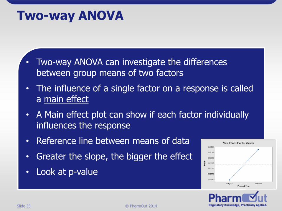
• Two-way ANOVA can investigate the differences between group means of two factors

• The influence of a single factor on a response is called a main effect

• A Main effect plot can show if each factor individually influences the response

• Reference line between means of data

• Greater the slope, the bigger the effect

• Look at p-value


Two-way ANOVA

• An interaction between factors is present when the change in the mean response across levels of one factor depends on the level of the 2nd factor

Interaction exists-lines not parallel No Interaction exists

Still check p-value from ANOVA output


Two-way ANOVA Hypothesis Test

• Hypothesis about whether group means are the same

• Can test each factor individually as well as the interaction between the 2 factors

• The null hypothesis states either that no main effect is present or that no interaction effect is present

• The alternative hypothesis states either that a main effect is present or that an interaction effect is present

• Look at F-statistic and p-value together. If p-value is >α, fail to reject the null hypothesis.


Design of Experiments (DoE)

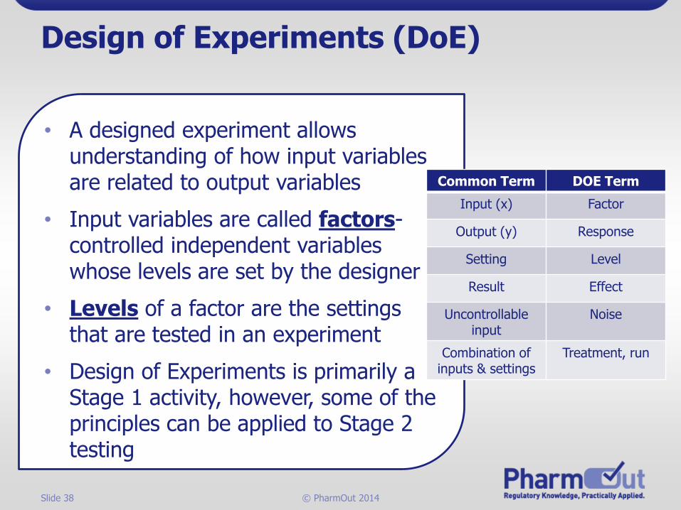
• A designed experiment allows understanding of how input variables are related to output variables

• Input variables are called factors-controlled independent variables whose levels are set by the designer

• Levels of a factor are the settings that are tested in an experiment

• Design of Experiments is primarily a Stage 1 activity, however, some of the principles can be applied to Stage 2 testing

Common Term DOE Term

Input (x) Factor

Output (y) Response

Setting Level

Result Effect

Uncontrollable input

Noise

Combination of inputs & settings

Treatment, run



• Factorial designs allow us to simultaneously study the effects of several factors on a process

• Varying the levels of the factors simultaneously rather than individually can save time and money and can also reveal the interactions between the factors

• “One factor at a time” (OFAT) experimental strategy does not consider the interaction between factors, has too many experiments & may never reveal the optimum combination of all variables.



• Determine the factors to evaluate-needs to come from process knowledge and statistical results

• Regression or ANOVA can identify factors that are significantly related to a response. DoE can clarify the effect of these factors.

• The levels at which the factors should be set at should be far enough apart so differences can be detected, but must be realistic settings

• Decide on the responses to measure (single/multiple)


Full Factorial Design

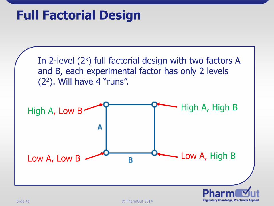
In 2-level (2k) full factorial design with two factors A and B, each experimental factor has only 2 levels (22). Will have 4 “runs”.

Low A, Low B

High A, Low B

Low A, High B

High A, High B



In 2-level (2k) full factorial design with three factors A, B and C, each experimental factor has 3 levels (23). Will have 8 “runs”.

Low A, Low B, Low C

High A, Low B, Low C

Low A, High B, Low C

High A, High B, Low C

Low A, Low B, High C

High A, Low B, High C High A, High B, High C

Low A, High B, High C



General full factorial designs are used when any experimental factor has more than two levels i.e. A is tested at two levels and B is tested at 3 levels



• A replicate is a duplicate run of the factor level combinations in an experiment. Replicates include sources of variability from setting up equipment, resetting factors and the natural variation in the process. It is the best estimate of experimental variability.

• It is preferable to randomise the order in which the runs are performed. This helps unknown sources of variation (i.e. environmental factors) that may affect the results.


Blocking

• When designing an experiment, good practice to incorporate known/suspected sources of variation

• Blocking reduces unwanted variation, which increases the precision of the experiment.

• Runs are then not completely randomised

• Runs are assigned to a logical collection, or block, and then randomised within the block

• Variation could include batches of raw materials, time, test equipment


Blocking

Example: Determine hardness of a PharmOdol® tablet

• Raw material from 2 different suppliers

• Previous experiences showed it as an uncontrollable factor-so a block in the experiment

• Important factors are speed and compression force, two-level factorial experiment with two factors run

• Block 1 represents raw material for supplier A

• Block 2 represents raw material for supplier B


Blocking

Blocks A: Machinespeed

B: Compression Force

Hardness (kp)

1 1000 20 5

1 3000 20 8

1 1000 40 4

1 3000 40 10

2 1000 20 6

2 3000 20 9

2 1000 40 4

2 3000 40 9

Block is not significant as p-value of 0.638. Raw material variability no impact on hardness


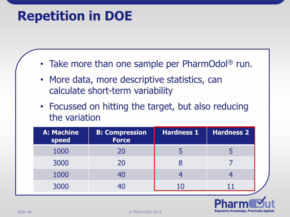
Repetition in DOE

• Take more than one sample per PharmOdol® run.

• More data, more descriptive statistics, can calculate short-term variability

• Focussed on hitting the target, but also reducing the variation

A: Machinespeed

B: Compression Force

Hardness 1 Hardness 2

1000 20 5 5

3000 20 8 7

1000 40 4 4

3000 40 10 11


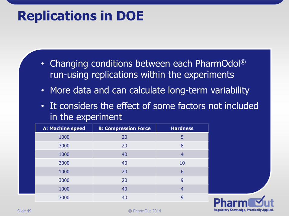
Replications in DOE

• Changing conditions between each PharmOdol®

run-using replications within the experiments

• More data and can calculate long-term variability

• It considers the effect of some factors not included in the experiment

A: Machine speed B: Compression Force Hardness

1000 20 5

3000 20 8

1000 40 4

3000 40 10

1000 20 6

3000 20 9

1000 40 4

3000 40 9


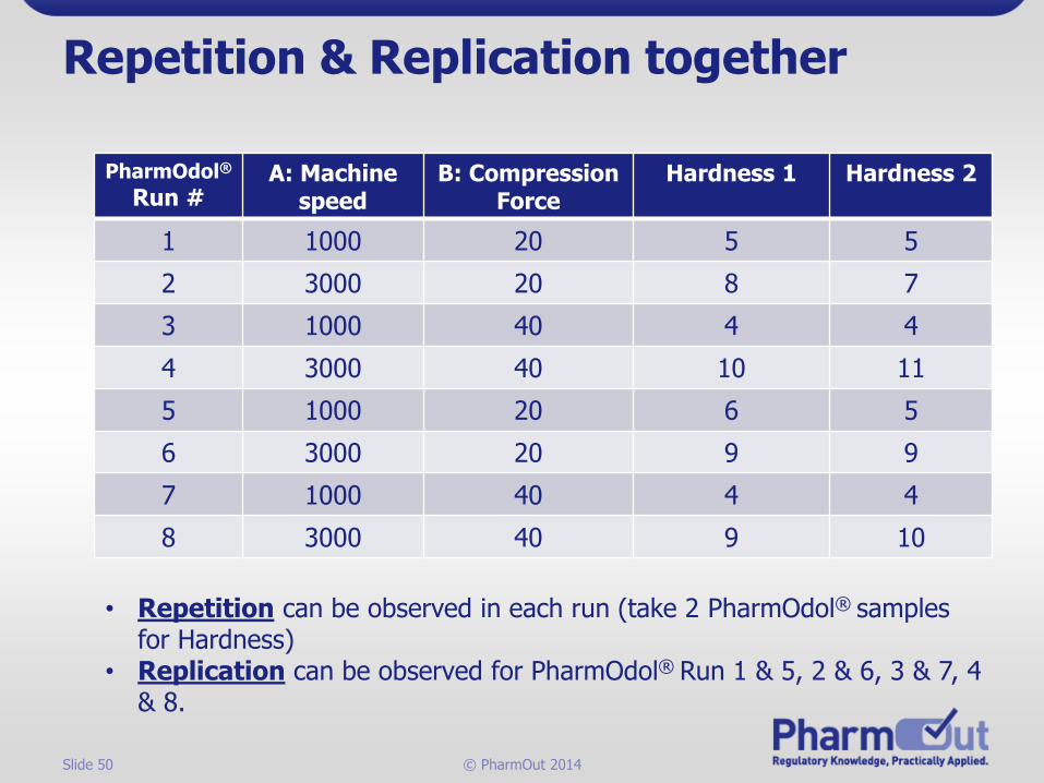
Repetition & Replication together

PharmOdol®

Run #A: Machine

speedB: Compression

ForceHardness 1 Hardness 2

1 1000 20 5 5

2 3000 20 8 7

3 1000 40 4 4

4 3000 40 10 11

5 1000 20 6 5

6 3000 20 9 9

7 1000 40 4 4

8 3000 40 9 10

• Repetition can be observed in each run (take 2 PharmOdol® samples for Hardness)

• Replication can be observed for PharmOdol® Run 1 & 5, 2 & 6, 3 & 7, 4 & 8.


Fractional Factorial Designs

23 Full Factorial design Half Fraction Factorial design

• Generally, not concerned with terms higher than the 2-way interaction as effects of high-order interactions can be negligible

• Good if limited resources

Minitab uses a design generator to determine how the fraction is selected


Activity 2: Statistics

Please complete the Blue Sheets as a group and return them to us

Please assign a Speaker/Scribe at

each table

If there are any questions, please ask!


Thank you for your time.Questions?

Ashley Isbel

[email protected]

Lead Consultant

www.pharmout.net

Date post:	23-Feb-2022
Category:	Documents
Upload:	others
View:	2 times
Download:	0 times

NVF III Session 2 Statistics

Documents