This work is licensed under a

Creative Commons Attribution-NonCommercial-NoDerivatives 4.0 International licence

Newcastle University ePrints - eprint.ncl.ac.uk

Obradors-Prats J, Rouainia M, Aplin AC, Crook AJL.

Stress and pore pressure histories in complex tectonic settings predicted with

coupled geomechanical-fluid flow models.

Marine and Petroleum Geology 2016, 76, 464-477.

Copyright:

© 2016. This manuscript version is made available under the CC-BY-NC-ND 4.0 license

DOI link to article:

http://dx.doi.org/10.1016/j.marpetgeo.2016.03.031

Date deposited:

06/07/2016

Embargo release date:

26 April 2017

Stress and pore pressure histories in complex tectonic

settings predicted with coupled geomechanical-fluid flow

models

Joshua Obradors-Pratsa, Mohamed Rouainiaa, Andrew C. Aplinb and Anthony J.L.

Crookc

aSchool of Civil Engineering and Geosciences, Newcastle University, Newcastle upon Tyne, NE1 7RU, UKbDepartment of Earth Sciences, Durham University, Durham, DH1 3LE, UK

cUniversity of Leeds, LS2 9JT, UK

Abstract

Most of the methods currently used for pore pressure prediction in sedimentary basins

assume one-dimensional compaction based on relationships between vertical effective

stress and porosity. These methods may be inaccurate in complex tectonic regimes

where stress tensors are variable. Modelling approaches for compaction adopted within

the geotechnical field account for both the full three-dimensional stress tensor and the

stress history. In this paper a coupled geomechanical-fluid flow model is used, along

with an advanced version of the Cam-Clay constitutive model, to investigate stress, pore

pressure and porosity in a Gulf of Mexico style mini-basin bounded by salt subjected to

lateral deformation. The modelled structure consists of two depocentres separated by

a salt diapir. 20% of horizontal shortening synchronous to basin sedimentation is im-

posed. An additional model accounting solely for the overpressure generated due to 1D

disequilibrium compaction is also defined. The predicted deformation regime in the two

depocentres of the mini-basin is one of tectonic lateral compression, in which the hori-

zontal effective stress is higher than the vertical effective stress. In contrast, sediments

above the central salt diapir show lateral extension and tectonic vertical compaction due

to the rise of the diapir. Compared to the 1D model, the horizontal shortening in the

mini-basin increases the predicted present-day overpressure by 50%, from 20 MPa to

30 MPa. The porosities predicted by the mini-basin models are used to perform 1D,

porosity-based pore pressure predictions. The 1D method underestimated overpressure

by up to 6 MPa at 3400 m depth (26% of the total overpressure) in the well located at the

basin depocentre and up to 3 MPa at 1900 m depth (34% of the total overpressure) in the

well located above the salt diapir. The results show how 2D/3D methods are required to

accurately predict overpressure in regions in which tectonic stresses are important.

Keywords: Numerical modelling, Forward modelling, Coupled geomechanics, Critical

state, Tectonic compaction, Pore pressure

Preprint submitted to Marine and Petroleum geology June 15, 2016

1. Introduction

Methods used to estimate present-day pore pressure in sedimentary basins and also

to model pore pressure evolution through time are largely based on relationships be-

tween stress, sediment compaction, the transient fluid flow regime and overpressure de-

velopment. The critical assumption in most of these methods is that porosity loss is

driven solely by the vertical effective stress exerted by the overburden, generally calcu-

lated as the lithostatic pressure minus the pore pressure (Terzaghi, 1923; Hubbert and

Rubey, 1959). This leads to quantifiable relationships between vertical effective stress

and porosity, or other porosity-dependent properties such as resistivity or sonic velocity

(Yang and Aplin, 2004; Zhang, 2011; Soleymani and Riahi, 2012; Zhang, 2013). These

methods, which are often termed ‘Equivalent Depth Methods’ (EDM), are most likely to

provide reasonable pore pressure predictions in simple, extensional tectonic settings in

which ‘disequilibrium compaction’, or the inability of the sediment to dewater relative to

the rate of sedimentation, is the dominant mechanism for overpressure generation. In

tectonically complex regions such as salt withdrawal mini-basins, toe thrusts and regions

dominated by regional compression, these standard pore pressure prediction methods

are unlikely to be accurate due to the true complexities of the stress tensor and its evolu-

tion through geologic time.

A range of approaches have been used to include the effects of 3D stress regimes into

models which simulate basin evolution and predict pore pressure. Couzens-Schultz and

Azbel (2014), for example, present an empirical pore pressure prediction model in the

NW Borneo-Sabah thrust-belt which includes a tectonic term that is a function of the dis-

tance to the axial planes of the major tectonic structures such as faults and folds. Whilst

numerical basin models can handle both 3D geometries and fluid flow, the description

of compaction is often one-dimensional, defined by relationships between porosity and

vertical effective stress. More recently, Cacas-Stenz et al. (2015) developed a basin

modelling approach in which the mean effective stress rather than the vertical effective

stress is assumed to drive the compaction process. The method assumes elastic strains

and the calculation of mean effective stress is performed by including a correction factor

related to Poisson’s ratio and the ratio of vertical to horizontal effective stress. Similarly,

Neumaier et al. (2014) proposed a methodology which integrates structural restoration

and basin modelling to improve petroleum charge and seal assessment in the Monagas

fold and thrust belt of Venezuela. One of the drawbacks of this method, however, is

the inaccurate description of compaction and overpressure generation, as compaction is

considered to be due only to the tectonic burial associated with thrusting in transient fluid

flow pathways.

The aim of this paper is to use a finite element geomechanical model to evaluate the

evolution of pore pressure in a setting where the assumption of 1D compaction is likely to

be inappropriate. Similar models have been used previously to evaluate deformation in

gravity-driven settings (e.g. Kjeldstad et al., 2003; Maghous et al., 2014), thrust faults and

basins located near salt diapirs (Albertz and Lingrey, 2012; Luo et al., 2012; Smart et al.,

2012), and also to model overpressure generation in complex stress regimes (Nikoli-

nakou et al., 2012; Thornton and Crook, 2014). An important aspect of these papers

was to incorporate advanced constitutive models that are capable of accurately describ-

ing the material rheology in a 3D simulation of an evolving basin. Here, we incorporate

similar methods but focus on pore pressure, specifically aiming to quantify the likely error

in pore pressure estimates caused by the erroneous assumption of 1D compaction (EDM

method) in complex stress regimes. To this end, finite element analyses of the sedimenta-

tion and evolution of a mini-basin bounded by salt subjected to lateral compression have

been undertaken, within the framework of a forward, coupled, geomechanical-fluid flow

modelling strategy. The resulting overpressure and porosity predictions are compared

with those obtained from the EDM. Focussing on a specific mini-basin has advantages

which include:

1. Implementation of a boundary-driven deformation approach in which the shape of

the basin is controlled by a prescribed displacement on a salt-sediment interface.

This gives the freedom to control the shape of the basin over time and to introduce

lateral compression within the model.

2. Salt can be considered impermeable so that the fluid system is isolated, simplifying

the definition of the boundary conditions.

3. Mini-basins are common targets for oil exploration (e.g. Gulf of Mexico), generating

published information which highlights the wide range of deformation styles that

mini-basins can experience due to the visco-plastic behaviour of salt (Marton et al.,

2000; Brun and Fort, 2004).

2. Modelled scenarios

This work aims to demonstrate the importance of using coupled geomechanical fluid

flow models to predict pore pressure where tectonic compaction is significant. The model

represents the evolution of a Gulf of Mexico style mini-basin bounded by salt in which

lateral deformation is introduced by prescribing a movement in the salt-sediment inter-

face. The model considers (a) simultaneous sedimentation, (b) vertical compaction due

to the load of the overburden and (c) tectonic compaction due to the movement of the

salt. Several models are built in order to assess the role of lateral deformation in sedi-

ment compaction and overpressure generation: 1) a base case mini-basin model; 2) a

model with its present day geometry defined to be laterally shortened relative to the base

case model and 3) a uniaxial burial model consisting of the deposition of a 2D column of

the same stratigraphy and sedimentation rates as the base case model. This latter model

estimates the overpressure generated solely by disequilibrium compaction. In addition,

the mini-basin models are simulated with both single lithology (clay) and mixed lithology

(clay and sand) stratigraphic columns in order to assess the contribution to overpressure

of high permeability layers. The complete list of all the models, with their corresponding

labels, is shown in Table 1.

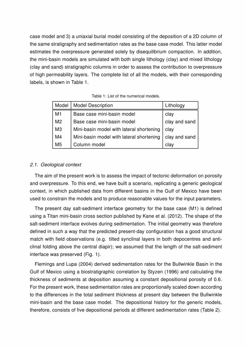
Table 1: List of the numerical models.

Model Model Description Lithology

M1 Base case mini-basin model clay

M2 Base case mini-basin model clay and sand

M3 Mini-basin model with lateral shortening clay

M4 Mini-basin model with lateral shortening clay and sand

M5 Column model clay

2.1. Geological context

The aim of the present work is to assess the impact of tectonic deformation on porosity

and overpressure. To this end, we have built a scenario, replicating a generic geological

context, in which published data from different basins in the Gulf of Mexico have been

used to constrain the models and to produce reasonable values for the input parameters.

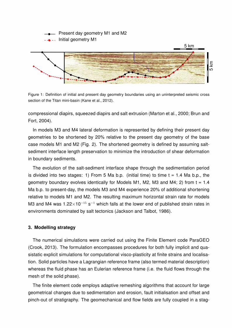
The present day salt-sediment interface geometry for the base case (M1) is defined

using a Titan mini-basin cross section published by Kane et al. (2012). The shape of the

salt-sediment interface evolves during sedimentation. The initial geometry was therefore

defined in such a way that the predicted present-day configuration has a good structural

match with field observations (e.g. tilted synclinal layers in both depocentres and anti-

clinal folding above the central diapir); we assumed that the length of the salt-sediment

interface was preserved (Fig. 1).

Flemings and Lupa (2004) derived sedimentation rates for the Bullwinkle Basin in the

Gulf of Mexico using a biostratigraphic correlation by Styzen (1996) and calculating the

thickness of sediments at deposition assuming a constant depositional porosity of 0.6.

For the present work, these sedimentation rates are proportionally scaled down according

to the differences in the total sediment thickness at present day between the Bullwinkle

mini-basin and the base case model. The depositional history for the generic models,

therefore, consists of five depositional periods at different sedimentation rates (Table 2).

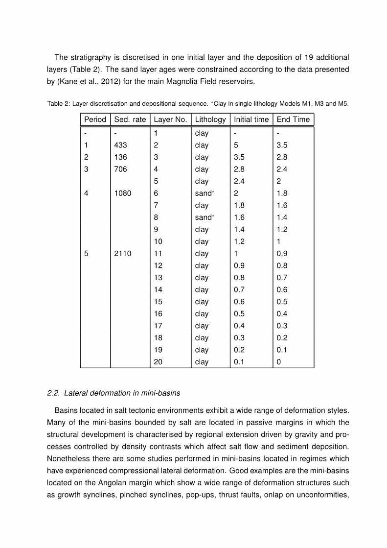
The stratigraphy is discretised in one initial layer and the deposition of 19 additional

layers (Table 2). The sand layer ages were constrained according to the data presented

by (Kane et al., 2012) for the main Magnolia Field reservoirs.

Table 2: Layer discretisation and depositional sequence. ∗Clay in single lithology Models M1, M3 and M5.

Period Sed. rate Layer No. Lithology Initial time End Time

- - 1 clay - -

1 433 2 clay 5 3.5

2 136 3 clay 3.5 2.8

3 706 4 clay 2.8 2.4

5 clay 2.4 2

4 1080 6 sand∗ 2 1.8

7 clay 1.8 1.6

8 sand∗ 1.6 1.4

9 clay 1.4 1.2

10 clay 1.2 1

5 2110 11 clay 1 0.9

12 clay 0.9 0.8

13 clay 0.8 0.7

14 clay 0.7 0.6

15 clay 0.6 0.5

16 clay 0.5 0.4

17 clay 0.4 0.3

18 clay 0.3 0.2

19 clay 0.2 0.1

20 clay 0.1 0

2.2. Lateral deformation in mini-basins

Basins located in salt tectonic environments exhibit a wide range of deformation styles.

Many of the mini-basins bounded by salt are located in passive margins in which the

structural development is characterised by regional extension driven by gravity and pro-

cesses controlled by density contrasts which affect salt flow and sediment deposition.

Nonetheless there are some studies performed in mini-basins located in regimes which

have experienced compressional lateral deformation. Good examples are the mini-basins

located on the Angolan margin which show a wide range of deformation structures such

as growth synclines, pinched synclines, pop-ups, thrust faults, onlap on unconformities,

Present day geometry M1 and M2

Initial geometry M1

5km

5 km

Figure 1: Definition of initial and present day geometry boundaries using an uninterpreted seismic cross

section of the Titan mini-basin (Kane et al., 2012).

compressional diapirs, squeezed diapirs and salt extrusion (Marton et al., 2000; Brun and

Fort, 2004).

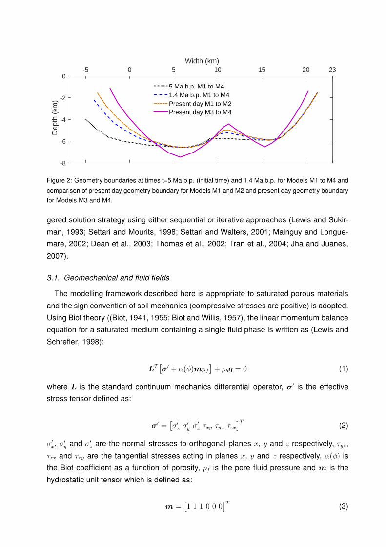
In models M3 and M4 lateral deformation is represented by defining their present day

geometries to be shortened by 20% relative to the present day geometry of the base

case models M1 and M2 (Fig. 2). The shortened geometry is defined by assuming salt-

sediment interface length preservation to minimize the introduction of shear deformation

in boundary sediments.

The evolution of the salt-sediment interface shape through the sedimentation period

is divided into two stages: 1) From 5 Ma b.p. (initial time) to time t = 1.4 Ma b.p., the

geometry boundary evolves identically for Models M1, M2, M3 and M4; 2) from t = 1.4

Ma b.p. to present-day, the models M3 and M4 experience 20% of additional shortening

relative to models M1 and M2. The resulting maximum horizontal strain rate for models

M3 and M4 was 1.22×10−15 s−1 which falls at the lower end of published strain rates in

environments dominated by salt tectonics (Jackson and Talbot, 1986).

3. Modelling strategy

The numerical simulations were carried out using the Finite Element code ParaGEO

(Crook, 2013). The formulation encompasses procedures for both fully implicit and qua-

sistatic explicit simulations for computational visco-plasticity at finite strains and localisa-

tion. Solid particles have a Lagrangian reference frame (also termed material description)

whereas the fluid phase has an Eulerian reference frame (i.e. the fluid flows through the

mesh of the solid phase).

The finite element code employs adaptive remeshing algorithms that account for large

geometrical changes due to sedimentation and erosion, fault initialisation and offset and

pinch-out of stratigraphy. The geomechanical and flow fields are fully coupled in a stag-

Width (km)-5 0 5 10 15 20 23

Dep

th (

km)

-8

-6

-4

-2

0

5 Ma b.p. M1 to M41.4 Ma b.p. M1 to M4Present day M1 to M2Present day M3 to M4

Figure 2: Geometry boundaries at times t=5 Ma b.p. (initial time) and 1.4 Ma b.p. for Models M1 to M4 and

comparison of present day geometry boundary for Models M1 and M2 and present day geometry boundary

for Models M3 and M4.

gered solution strategy using either sequential or iterative approaches (Lewis and Sukir-

man, 1993; Settari and Mourits, 1998; Settari and Walters, 2001; Mainguy and Longue-

mare, 2002; Dean et al., 2003; Thomas et al., 2002; Tran et al., 2004; Jha and Juanes,

2007).

3.1. Geomechanical and fluid fields

The modelling framework described here is appropriate to saturated porous materials

and the sign convention of soil mechanics (compressive stresses are positive) is adopted.

Using Biot theory ((Biot, 1941, 1955; Biot and Willis, 1957), the linear momentum balance

equation for a saturated medium containing a single fluid phase is written as (Lewis and

Schrefler, 1998):

LT[

σ′ + α(φ)mpf]

+ ρbg = 0 (1)

where L is the standard continuum mechanics differential operator, σ′ is the effective

stress tensor defined as:

σ′ =[

σ′

x σ′

y σ′

z τxy τyz τzx]T

(2)

σ′

x, σ′

y and σ′

z are the normal stresses to orthogonal planes x, y and z respectively, τyz,

τzx and τxy are the tangential stresses acting in planes x, y and z respectively, α(φ) is

the Biot coefficient as a function of porosity, pf is the pore fluid pressure and m is the

hydrostatic unit tensor which is defined as:

m =[

1 1 1 0 0 0]T

(3)

ρb is the saturated bulk mass density which is defined as:

ρb = (1− φ)ρs + φρf (4)

in which ρs and ρf are the solid and fluid densities respectively and g is the gravitational

vector.

Effective stress is the component of the total stress exerted by the solid matrix. It is

defined as:

σ′ = σ − α(φ)mpf (5)

where σ is the total stress tensor.

The Biot coefficient α(φ) indicates the contribution of the pore fluid to the decrease

in the effective stresses. It is expected to decrease with a decrease in porosity so that

for the same total stress and pore pressure lower values of the Biot coefficient result

in higher effective stress (higher stress transferred by grain to grain contact). For the

current application we have assumed a constant value of α(φ) = α = 1 which results in

a Terzaghi definition of the effective stress to facilitate a latter comparison between pore

pressure solution provided by the numerical models and solution obtained by standard

porosity based pore prediction methods widely used in the industry.

Fluid transport over geological time frames is modelled by the single phase Darcy flow

equation as defined in (Lewis and Schrefler, 1998):

div

[

(k(φ)

µf

(

∇pf − ρfg)

]

=

[

φ

Kf+

(

α(φ)− φ)

Ks

]

∂pf

∂t+

α(φ)

(1− φ)

∂φ

∂t(6)

where Kf is the fluid stiffness, Ks is the solid grains stiffness, µf is the fluid viscosity

and k(φ) is the permeability tensor which is a function of porosity. Note that the last term

in Eq. 6 represents the fluid flow due to a change in porosity and provides the coupling

between the mechanical and flow fields.

3.2. Constitutive equations

An advanced non-associative version of a Cam clay-based critical state constitutive

model (denoted SR4) is adopted that is able to simulate strain hardening (increase in

sediment strength due to compaction), strain softening (sediment strength decrease) and

shear strain at constant volume once a critical state is reached (Wood, 1990). The evo-

lution of the state variables of the rock formation are computed simultaneously (material

state boundary surface, sediment permeability, fluid properties, fault formation and prop-

agation, etc).

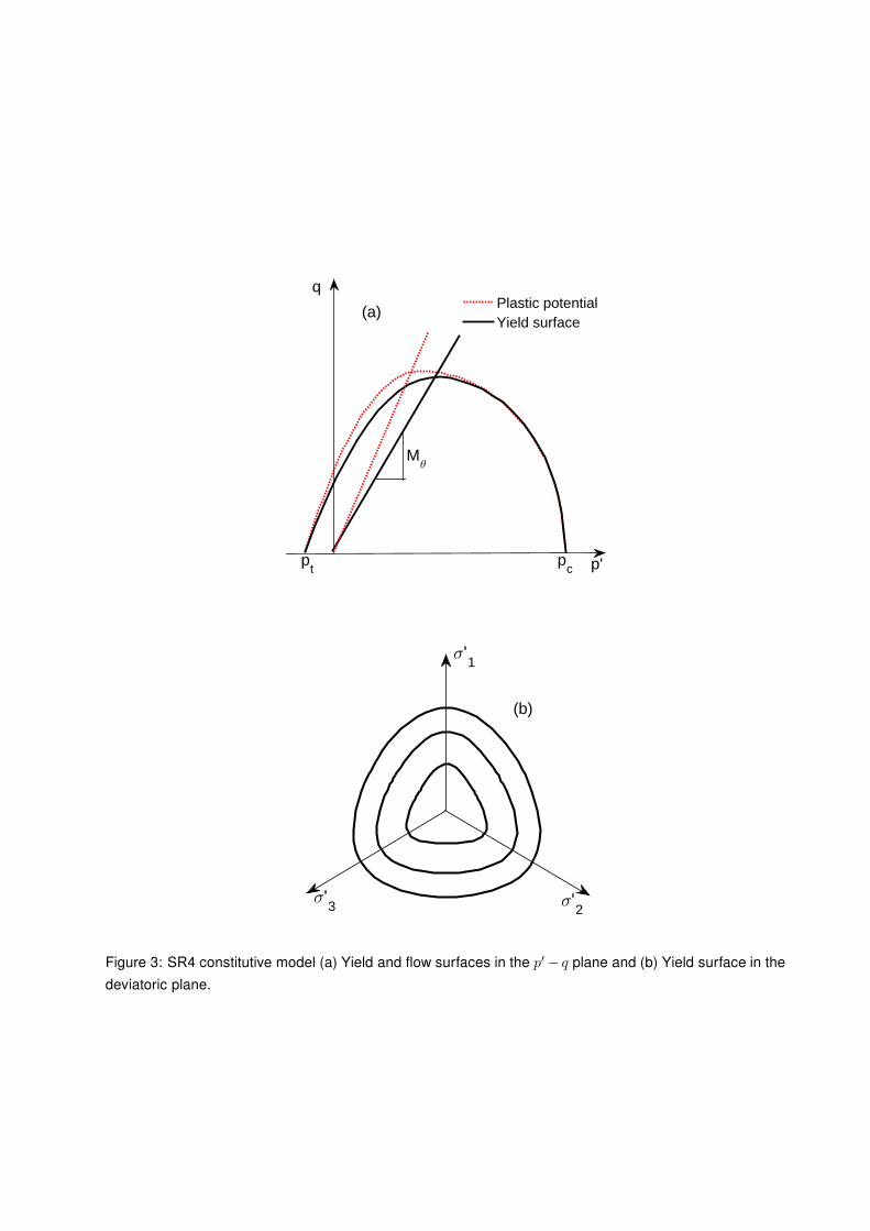
The state boundary surface for the novel SR4 model relies on the existence of a smooth

three-invariant surface composed of two functions that intersect in a continuous manner

at the point of maximum deviatoric stress (Fig. 3). The shear side is defined using the

SR3 surface (Crook et al., 2006) while the compression side is defined by an ellipse in a

similar manner as the standard Cam clay model (Wood, 1990):

φ(p′, εpv) = g(θ, p′)q + (p′ − pt) tanβ

[

(p′ − pc)

(pt − pc)

]1/n

(7)

for p′ ≥ pφpeak and

φ(p′, εpv) =[

g(θ, p′)]2q2 −M2

φp2φpeak

[

1−(φpeak − p′)2

(φpeak − pc)2

]

(8)

for p′ < pφpeak

where p′ is the effective mean stress, q is the deviatoric stress. pt is the tensile inter-

cept of the yield surface with the hydrostatic axis, pc is the pre-consolidation pressure or

compressive intercept of the yield surface with the hydrostatic axis, pφpeak is the effective

mean stress corresponding to the peak value of q for the yield surface, εpv is the plastic

volumetric strain, Mφ is the slope of the line that intersects both the origin of the p′ − q

space and the q peak value for the yield surface, β and n are material constants which

define the shape of the yield surface in the p′ − q plane, θ is the lode angle and g(θ, p′) is

a function that controls the shape of the yield surface in the deviatoric plane.

The flow potential surface has the same form of the state boundary surface but is

defined with two different parameters. This enables the critical state line (CSL) to be

defined to intersect the state boundary surface on the shear side, as opposed to the

peak stress (Fig. 3), which is consistent with experimental observations for clays. The

flow potential surface is defined as:

ψ(p′, εpv) = q + (p′ − pt) tanψ

[

(p′ − pc)

(pt − pc)

](1/m)

(9)

for p′ ≥ pψpeakand

ψ(p′, εpv) = q2 −M2p2ψpeak

[

1−(pψpeak

− p′)2

(pψpeak− pc)2

]

(10)

for p′ < pψpeak

where M is the slope of the critical state line, pψpeakis the effective mean stress corre-

sponding to the peak value of q for the flow potential surface, and ψ and m are material

constants which define the shape of the flow potential surface in the p′ − q plane. Note

Plastic potentialYield surface

Mθ

p'pt

pc

(a)

q

(b)

σ'1

σ'2

σ'3

Figure 3: SR4 constitutive model (a) Yield and flow surfaces in the p′ − q plane and (b) Yield surface in the

deviatoric plane.

that the flow potential surface does not have any deviatoric correction term (as opposed

to the yield surface) as it is circular in the deviatoric plane for all values of pc.

Appendix A and Table A.1 give the remaining equations of the SR4 constitutive model

used to simulate sediment rheology along with the material properties used to for clay

and sand and their respective porosity-permeability curves.

3.3. Boundary conditions for the models

The evolution of the salt-sediment interface of the mini basins is fully prescribed and

occurs synchronously to sedimentation. The approach consisted in discretising the salt-

sediment interface into 25 nodes which delimitate 24 lines. The x and y coordinates of the

25 nodes were prescribed at target paleo-times according to the salt-sediment interface

shape. Then, the shape evolution between two prescribed paleo-times is governed by a

linear displacement in the nodes with constant velocity which is automatically computed

as the change in x and y coordinates for each node between those prescribed paleotimes.

The prescribed present day salt-sediment interface for the models with 20% of lateral

shortening (models M3 and M4) was defined preserving the boundary length relative

to the boundary length in models M1 and M2. The procedure for the definition of the

present day salt-sediment interface shape for models M3 and M4 was as follows: 1)

The present day shape of the salt-sediment interface for models M1 and M2 was taken

as a benchmark. 2) A central node located in the central salt diapir is selected. 3)

The x coordinate for each node of the salt sediment interface is modified in such a way

that the horizontal distance to the selected central node is reduced by 10%. 4) The y

coordinates of all nodes are modified to preserve the boundary length relative to Models

M1 and M2. By assuming constant boundary length preservation we aim to minimize the

introduction of shear strain on boundary sediments. The resulting present-day geometry

is horizontally shortened by 20% relative to the present-day geometries of Models M1

and M2 (Fig. 2).

Salt can be considered impermeable and therefore a non-flow boundary condition is

imposed at the salt-sediment interface. The top sediment surface is treated as a free

surface by imposing free displacement and zero overpressure boundary conditions.

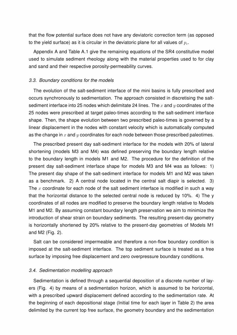
3.4. Sedimentation modelling approach

Sedimentation is defined through a sequential deposition of a discrete number of lay-

ers (Fig. 4) by means of a sedimentation horizon, which is assumed to be horizontal,

with a prescribed upward displacement defined according to the sedimentation rate. At

the beginning of each depositional stage (Initial time for each layer in Table 2) the area

delimited by the current top free surface, the geometry boundary and the sedimentation

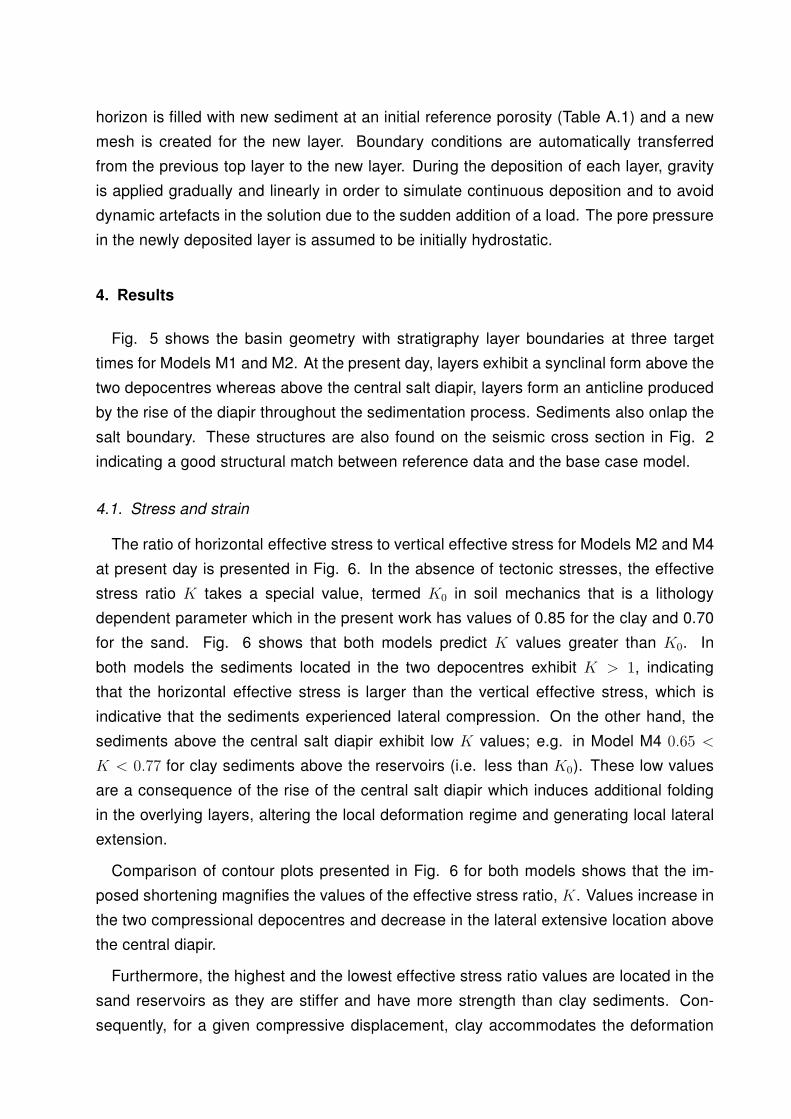
horizon is filled with new sediment at an initial reference porosity (Table A.1) and a new

mesh is created for the new layer. Boundary conditions are automatically transferred

from the previous top layer to the new layer. During the deposition of each layer, gravity

is applied gradually and linearly in order to simulate continuous deposition and to avoid

dynamic artefacts in the solution due to the sudden addition of a load. The pore pressure

in the newly deposited layer is assumed to be initially hydrostatic.

4. Results

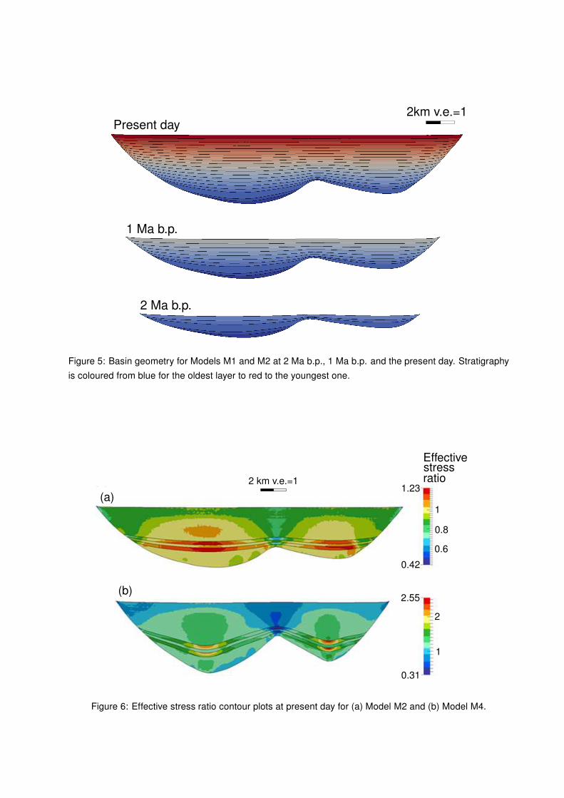
Fig. 5 shows the basin geometry with stratigraphy layer boundaries at three target

times for Models M1 and M2. At the present day, layers exhibit a synclinal form above the

two depocentres whereas above the central salt diapir, layers form an anticline produced

by the rise of the diapir throughout the sedimentation process. Sediments also onlap the

salt boundary. These structures are also found on the seismic cross section in Fig. 2

indicating a good structural match between reference data and the base case model.

4.1. Stress and strain

The ratio of horizontal effective stress to vertical effective stress for Models M2 and M4

at present day is presented in Fig. 6. In the absence of tectonic stresses, the effective

stress ratio K takes a special value, termed K0 in soil mechanics that is a lithology

dependent parameter which in the present work has values of 0.85 for the clay and 0.70

for the sand. Fig. 6 shows that both models predict K values greater than K0. In

both models the sediments located in the two depocentres exhibit K > 1, indicating

that the horizontal effective stress is larger than the vertical effective stress, which is

indicative that the sediments experienced lateral compression. On the other hand, the

sediments above the central salt diapir exhibit low K values; e.g. in Model M4 0.65 <

K < 0.77 for clay sediments above the reservoirs (i.e. less than K0). These low values

are a consequence of the rise of the central salt diapir which induces additional folding

in the overlying layers, altering the local deformation regime and generating local lateral

extension.

Comparison of contour plots presented in Fig. 6 for both models shows that the im-

posed shortening magnifies the values of the effective stress ratio, K. Values increase in

the two compressional depocentres and decrease in the lateral extensive location above

the central diapir.

Furthermore, the highest and the lowest effective stress ratio values are located in the

sand reservoirs as they are stiffer and have more strength than clay sediments. Con-

sequently, for a given compressive displacement, clay accommodates the deformation

Layer 1

Layer 2

Layer 2

Layer 1

Layer 3

Layer 2

Layer 1

t0

t0 <t<tf

tf

d∗

d∗

d∗

SH

SH

SH

Sa

se

Layer 3

ment

-lt

inte

r face

di

Sa

sem

ent

-lt

inte

r face

di

Sa

sem

ent

-lt

inte

r face

di

(a)

(b)

(c)

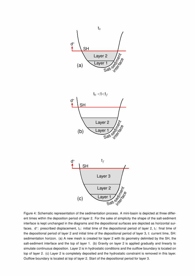
Figure 4: Schematic representation of the sedimentation process. A mini-basin is depicted at three differ-

ent times within the deposition period of layer 2. For the sake of simplicity the shape of the salt-sediment

interface is kept unchanged in the diagrams and the depositional surfaces are depicted as horizontal sur-

faces. d∗: prescribed displacement, t0: initial time of the depositional period of layer 2, tf : final time of

the depositional period of layer 2 and initial time of the depositional period of layer 3, t: current time, SH:

sedimentation horizon. (a) A new mesh is created for layer 2 with its geometry delimited by the SH, the

salt-sediment interface and the top of layer 1. (b) Gravity on layer 2 is applied gradually and linearly to

simulate continuous deposition. Layer 2 is in hydrostatic conditions and the outflow boundary is located on

top of layer 2. (c) Layer 2 is completely deposited and the hydrostatic constraint is removed in this layer.

Outflow boundary is located at top of layer 2. Start of the depositional period for layer 3.

Present day

2 Ma b.p.

1 Ma b.p.

2km v.e.=1

Figure 5: Basin geometry for Models M1 and M2 at 2 Ma b.p., 1 Ma b.p. and the present day. Stratigraphy

is coloured from blue for the oldest layer to red to the youngest one.

2 km v.e.=1

(a)

(b)

Effectivestress

1.23

0.42

ratio

2.55

0.31

2

1

1

0.8

0.6

Figure 6: Effective stress ratio contour plots at present day for (a) Model M2 and (b) Model M4.

more readily than the stiffer sand, which absorbs more of the stress. This resembles

a situation of applying a prescribed displacement on two parallel springs with different

stiffness.

(b)

(a)

2 km v.e.=1

0.336

-0.368

0.2

0

-0.2

-0.045

-0.2

-0.4

-0.6

Horizontalstrain

Verticalstrain

-0.92

-0.8

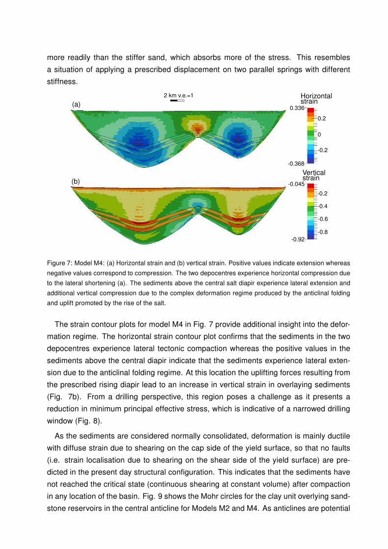
Figure 7: Model M4: (a) Horizontal strain and (b) vertical strain. Positive values indicate extension whereas

negative values correspond to compression. The two depocentres experience horizontal compression due

to the lateral shortening (a). The sediments above the central salt diapir experience lateral extension and

additional vertical compression due to the complex deformation regime produced by the anticlinal folding

and uplift promoted by the rise of the salt.

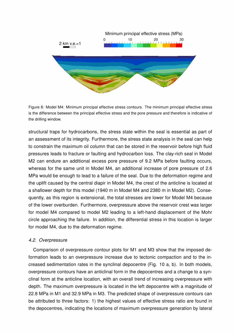
The strain contour plots for model M4 in Fig. 7 provide additional insight into the defor-

mation regime. The horizontal strain contour plot confirms that the sediments in the two

depocentres experience lateral tectonic compaction whereas the positive values in the

sediments above the central diapir indicate that the sediments experience lateral exten-

sion due to the anticlinal folding regime. At this location the uplifting forces resulting from

the prescribed rising diapir lead to an increase in vertical strain in overlaying sediments

(Fig. 7b). From a drilling perspective, this region poses a challenge as it presents a

reduction in minimum principal effective stress, which is indicative of a narrowed drilling

window (Fig. 8).

As the sediments are considered normally consolidated, deformation is mainly ductile

with diffuse strain due to shearing on the cap side of the yield surface, so that no faults

(i.e. strain localisation due to shearing on the shear side of the yield surface) are pre-

dicted in the present day structural configuration. This indicates that the sediments have

not reached the critical state (continuous shearing at constant volume) after compaction

in any location of the basin. Fig. 9 shows the Mohr circles for the clay unit overlying sand-

stone reservoirs in the central anticline for Models M2 and M4. As anticlines are potential

2 km v.e.=1

Minimum principal effective stress (MPa)

0 10 20 30

Figure 8: Model M4: Minimum principal effective stress contours. The minimum principal effective stress

is the difference between the principal effective stress and the pore pressure and therefore is indicative of

the drilling window.

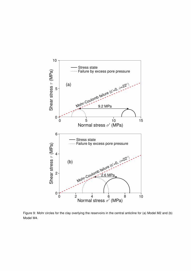
structural traps for hydrocarbons, the stress state within the seal is essential as part of

an assessment of its integrity. Furthermore, the stress state analysis in the seal can help

to constrain the maximum oil column that can be stored in the reservoir before high fluid

pressures leads to fracture or faulting and hydrocarbon loss. The clay-rich seal in Model

M2 can endure an additional excess pore pressure of 9.2 MPa before faulting occurs,

whereas for the same unit in Model M4, an additional increase of pore pressure of 2.6

MPa would be enough to lead to a failure of the seal. Due to the deformation regime and

the uplift caused by the central diapir in Model M4, the crest of the anticline is located at

a shallower depth for this model (1940 m in Model M4 and 2380 m in Model M2). Conse-

quently, as this region is extensional, the total stresses are lower for Model M4 because

of the lower overburden. Furthermore, overpressure above the reservoir crest was larger

for model M4 compared to model M2 leading to a left-hand displacement of the Mohr

circle approaching the failure. In addition, the differential stress in this location is larger

for model M4, due to the deformation regime.

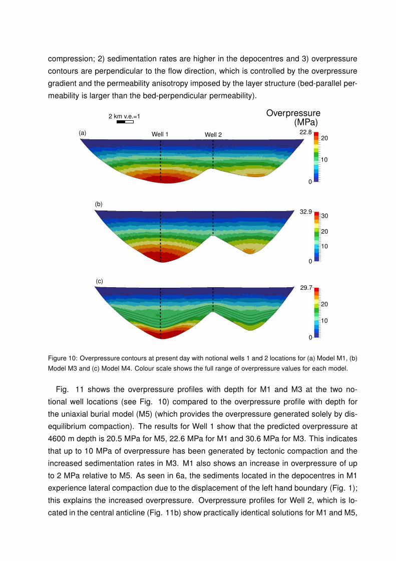
4.2. Overpressure

Comparison of overpressure contour plots for M1 and M3 show that the imposed de-

formation leads to an overpressure increase due to tectonic compaction and to the in-

creased sedimentation rates in the synclinal depocentre (Fig. 10 a, b). In both models,

overpressure contours have an anticlinal form in the depocentres and a change to a syn-

clinal form at the anticline location, with an overall trend of increasing overpressure with

depth. The maximum overpressure is located in the left depocentre with a magnitude of

22.8 MPa in M1 and 32.9 MPa in M3. The predicted shape of overpressure contours can

be attributed to three factors: 1) the highest values of effective stress ratio are found in

the depocentres, indicating the locations of maximum overpressure generation by lateral

Sh

ea

rstr

essτ

(MP

a) Stress state

Failure by excess pore pressure

Mohr-Coulomb failure (c’=0, φ=22

o )

9.2 MPa

10 155

5

10

0

Normal stress σ′ (MPa)

0

Stress stateFailure by excess pore pressure

Mohr-Coulomb failure

(c’=0, φ=22

o )

Normal stress σ′ (MPa)

Sh

ea

rstr

essτ

(MP

a)

0 2 4 6 8 10

4

6

2.6 MPa

(a)

(b)

2

0

Figure 9: Mohr circles for the clay overlying the reservoirs in the central anticline for (a) Model M2 and (b)

Model M4.

compression; 2) sedimentation rates are higher in the depocentres and 3) overpressure

contours are perpendicular to the flow direction, which is controlled by the overpressure

gradient and the permeability anisotropy imposed by the layer structure (bed-parallel per-

meability is larger than the bed-perpendicular permeability).

Well 1 Well 2

(c)

(b)

(a)

Overpressure(MPa)

10

0

22.820

10

0

32.930

20

10

0

29.7

20

2 km v.e.=1

Figure 10: Overpressure contours at present day with notional wells 1 and 2 locations for (a) Model M1, (b)

Model M3 and (c) Model M4. Colour scale shows the full range of overpressure values for each model.

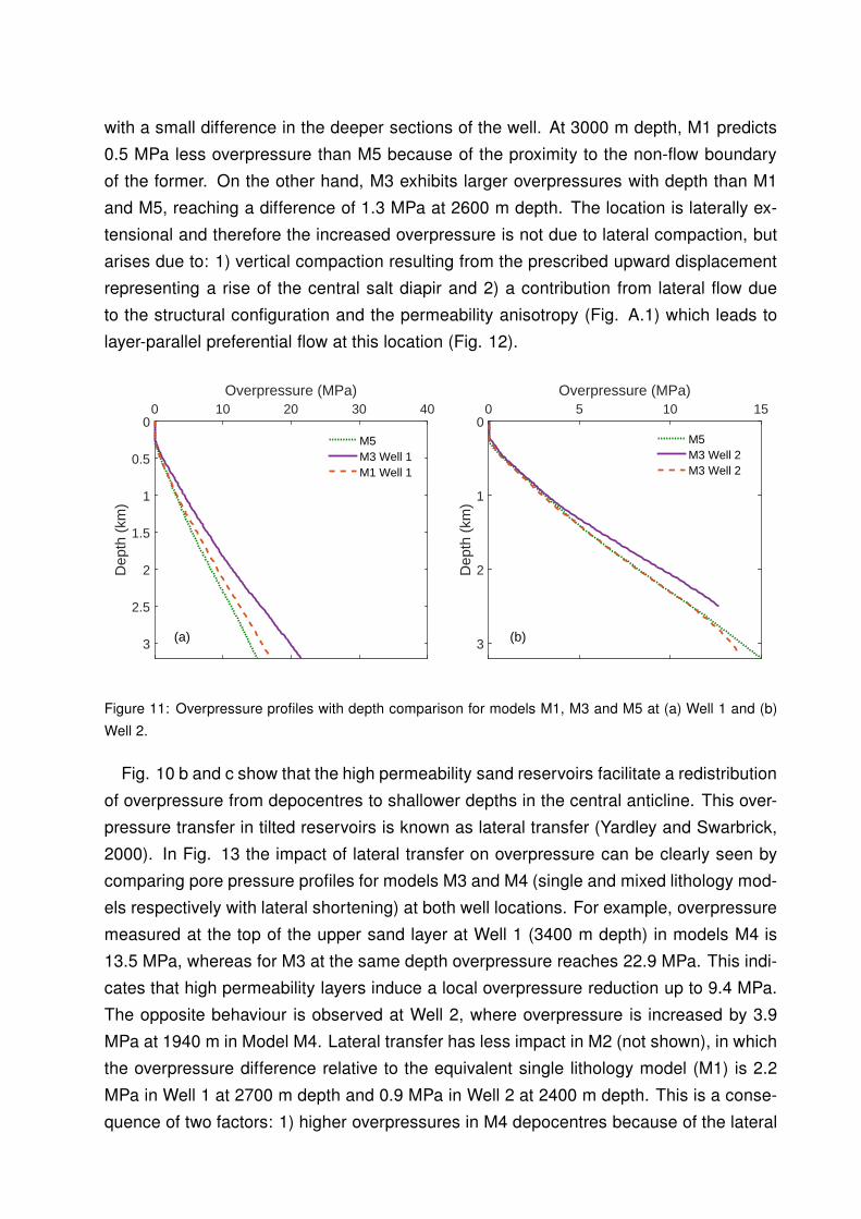
Fig. 11 shows the overpressure profiles with depth for M1 and M3 at the two no-

tional well locations (see Fig. 10) compared to the overpressure profile with depth for

the uniaxial burial model (M5) (which provides the overpressure generated solely by dis-

equilibrium compaction). The results for Well 1 show that the predicted overpressure at

4600 m depth is 20.5 MPa for M5, 22.6 MPa for M1 and 30.6 MPa for M3. This indicates

that up to 10 MPa of overpressure has been generated by tectonic compaction and the

increased sedimentation rates in M3. M1 also shows an increase in overpressure of up

to 2 MPa relative to M5. As seen in 6a, the sediments located in the depocentres in M1

experience lateral compaction due to the displacement of the left hand boundary (Fig. 1);

this explains the increased overpressure. Overpressure profiles for Well 2, which is lo-

cated in the central anticline (Fig. 11b) show practically identical solutions for M1 and M5,

with a small difference in the deeper sections of the well. At 3000 m depth, M1 predicts

0.5 MPa less overpressure than M5 because of the proximity to the non-flow boundary

of the former. On the other hand, M3 exhibits larger overpressures with depth than M1

and M5, reaching a difference of 1.3 MPa at 2600 m depth. The location is laterally ex-

tensional and therefore the increased overpressure is not due to lateral compaction, but

arises due to: 1) vertical compaction resulting from the prescribed upward displacement

representing a rise of the central salt diapir and 2) a contribution from lateral flow due

to the structural configuration and the permeability anisotropy (Fig. A.1) which leads to

layer-parallel preferential flow at this location (Fig. 12).

Overpressure (MPa)0 10 20 30 40

Dep

th (

km)

0

0.5

1

1.5

2

2.5

3

M5M3 Well 1 M1 Well 1

Overpressure (MPa)0 5 10 15

Dep

th (

km)

0

1

2

3

M5M3 Well 2M3 Well 2

(b)(a)

Figure 11: Overpressure profiles with depth comparison for models M1, M3 and M5 at (a) Well 1 and (b)

Well 2.

Fig. 10 b and c show that the high permeability sand reservoirs facilitate a redistribution

of overpressure from depocentres to shallower depths in the central anticline. This over-

pressure transfer in tilted reservoirs is known as lateral transfer (Yardley and Swarbrick,

2000). In Fig. 13 the impact of lateral transfer on overpressure can be clearly seen by

comparing pore pressure profiles for models M3 and M4 (single and mixed lithology mod-

els respectively with lateral shortening) at both well locations. For example, overpressure

measured at the top of the upper sand layer at Well 1 (3400 m depth) in models M4 is

13.5 MPa, whereas for M3 at the same depth overpressure reaches 22.9 MPa. This indi-

cates that high permeability layers induce a local overpressure reduction up to 9.4 MPa.

The opposite behaviour is observed at Well 2, where overpressure is increased by 3.9

MPa at 1940 m in Model M4. Lateral transfer has less impact in M2 (not shown), in which

the overpressure difference relative to the equivalent single lithology model (M1) is 2.2

MPa in Well 1 at 2700 m depth and 0.9 MPa in Well 2 at 2400 m depth. This is a conse-

quence of two factors: 1) higher overpressures in M4 depocentres because of the lateral

1 km v.e.=1

4 km v.e.=1

10

0 32.9

20

Overpressure (MPa)

30

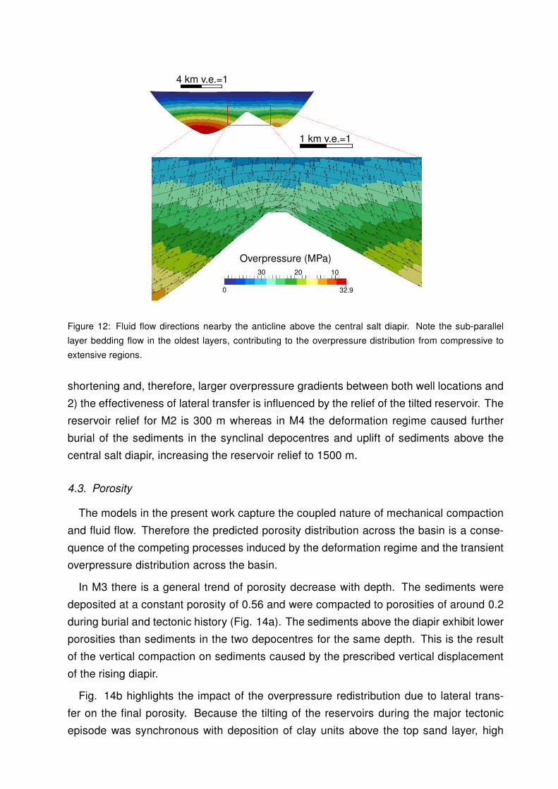
Figure 12: Fluid flow directions nearby the anticline above the central salt diapir. Note the sub-parallel

layer bedding flow in the oldest layers, contributing to the overpressure distribution from compressive to

extensive regions.

shortening and, therefore, larger overpressure gradients between both well locations and

2) the effectiveness of lateral transfer is influenced by the relief of the tilted reservoir. The

reservoir relief for M2 is 300 m whereas in M4 the deformation regime caused further

burial of the sediments in the synclinal depocentres and uplift of sediments above the

central salt diapir, increasing the reservoir relief to 1500 m.

4.3. Porosity

The models in the present work capture the coupled nature of mechanical compaction

and fluid flow. Therefore the predicted porosity distribution across the basin is a conse-

quence of the competing processes induced by the deformation regime and the transient

overpressure distribution across the basin.

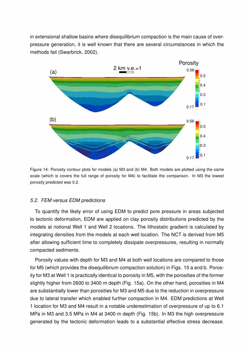
In M3 there is a general trend of porosity decrease with depth. The sediments were

deposited at a constant porosity of 0.56 and were compacted to porosities of around 0.2

during burial and tectonic history (Fig. 14a). The sediments above the diapir exhibit lower

porosities than sediments in the two depocentres for the same depth. This is the result

of the vertical compaction on sediments caused by the prescribed vertical displacement

of the rising diapir.

Fig. 14b highlights the impact of the overpressure redistribution due to lateral trans-

fer on the final porosity. Because the tilting of the reservoirs during the major tectonic

episode was synchronous with deposition of clay units above the top sand layer, high

Overpressure (MPa)0 10 20 30 40

Dep

th (

km)

0

1

2

3

4

5

M4 Well 1 M3 Well 1

Overpressure (MPa)0 5 10 15 20

Dep

th (

km)

0

1

2

3

M4 Well 2M3 Well 2

(b)(a)

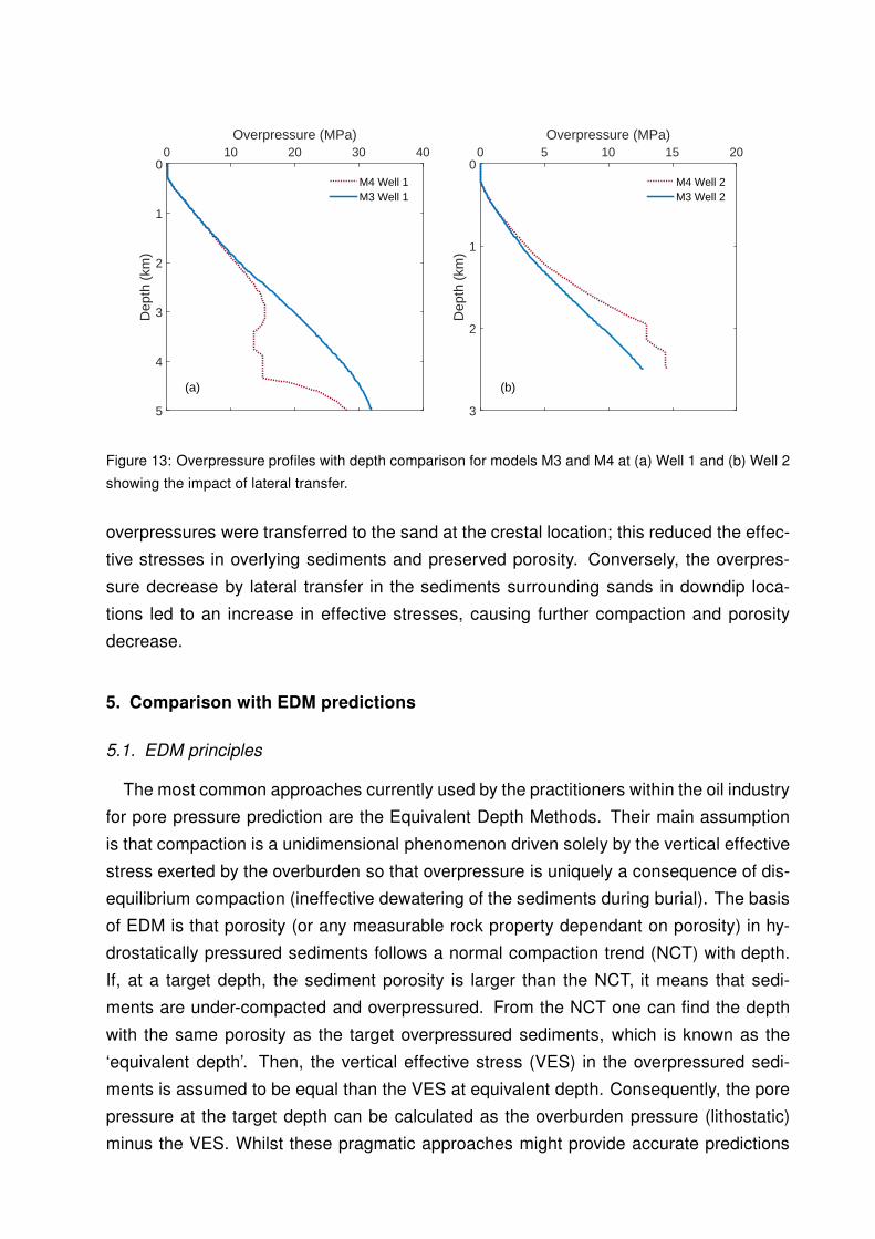
Figure 13: Overpressure profiles with depth comparison for models M3 and M4 at (a) Well 1 and (b) Well 2

showing the impact of lateral transfer.

overpressures were transferred to the sand at the crestal location; this reduced the effec-

tive stresses in overlying sediments and preserved porosity. Conversely, the overpres-

sure decrease by lateral transfer in the sediments surrounding sands in downdip loca-

tions led to an increase in effective stresses, causing further compaction and porosity

decrease.

5. Comparison with EDM predictions

5.1. EDM principles

The most common approaches currently used by the practitioners within the oil industry

for pore pressure prediction are the Equivalent Depth Methods. Their main assumption

is that compaction is a unidimensional phenomenon driven solely by the vertical effective

stress exerted by the overburden so that overpressure is uniquely a consequence of dis-

equilibrium compaction (ineffective dewatering of the sediments during burial). The basis

of EDM is that porosity (or any measurable rock property dependant on porosity) in hy-

drostatically pressured sediments follows a normal compaction trend (NCT) with depth.

If, at a target depth, the sediment porosity is larger than the NCT, it means that sedi-

ments are under-compacted and overpressured. From the NCT one can find the depth

with the same porosity as the target overpressured sediments, which is known as the

‘equivalent depth’. Then, the vertical effective stress (VES) in the overpressured sedi-

ments is assumed to be equal than the VES at equivalent depth. Consequently, the pore

pressure at the target depth can be calculated as the overburden pressure (lithostatic)

minus the VES. Whilst these pragmatic approaches might provide accurate predictions

in extensional shallow basins where disequilibrium compaction is the main cause of over-

pressure generation, it is well known that there are several circumstances in which the

methods fail (Swarbrick, 2002).

2 km v.e.=1Porosity

0.5

0.56

0.170.1

0.4

0.3

0.5

0.56

0.170.1

0.4

0.3

(a)

(b)

Figure 14: Porosity contour plots for models (a) M3 and (b) M4. Both models are plotted using the same

scale (which is covers the full range of porosity for M4) to facilitate the comparison. In M3 the lowest

porosity predicted was 0.2.

5.2. FEM versus EDM predictions

To quantify the likely error of using EDM to predict pore pressure in areas subjected

to tectonic deformation, EDM are applied on clay porosity distributions predicted by the

models at notional Well 1 and Well 2 locations. The lithostatic gradient is calculated by

integrating densities from the models at each well location. The NCT is derived from M5

after allowing sufficient time to completely dissipate overpressures, resulting in normally

compacted sediments.

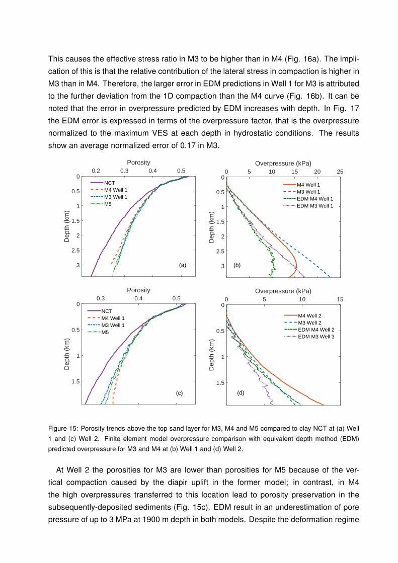
Porosity values with depth for M3 and M4 at both well locations are compared to those

for M5 (which provides the disequilibrium compaction solution) in Figs. 15 a and b. Poros-

ity for M3 at Well 1 is practically identical to porosity in M5, with the porosities of the former

slightly higher from 2600 to 3400 m depth (Fig. 15a). On the other hand, porosities in M4

are substantially lower than porosities for M3 and M5 due to the reduction in overpressure

due to lateral transfer which enabled further compaction in M4. EDM predictions at Well

1 location for M3 and M4 result in a notable underestimation of overpressure of up to 6.1

MPa in M3 and 3.5 MPa in M4 at 3400 m depth (Fig. 15b). In M3 the high overpressure

generated by the tectonic deformation leads to a substantial effective stress decrease.

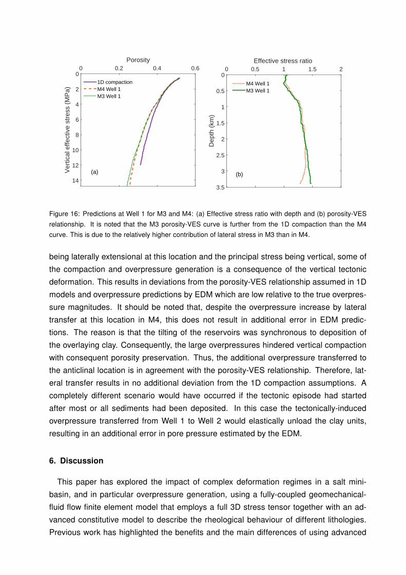
This causes the effective stress ratio in M3 to be higher than in M4 (Fig. 16a). The impli-

cation of this is that the relative contribution of the lateral stress in compaction is higher in

M3 than in M4. Therefore, the larger error in EDM predictions in Well 1 for M3 is attributed

to the further deviation from the 1D compaction than the M4 curve (Fig. 16b). It can be

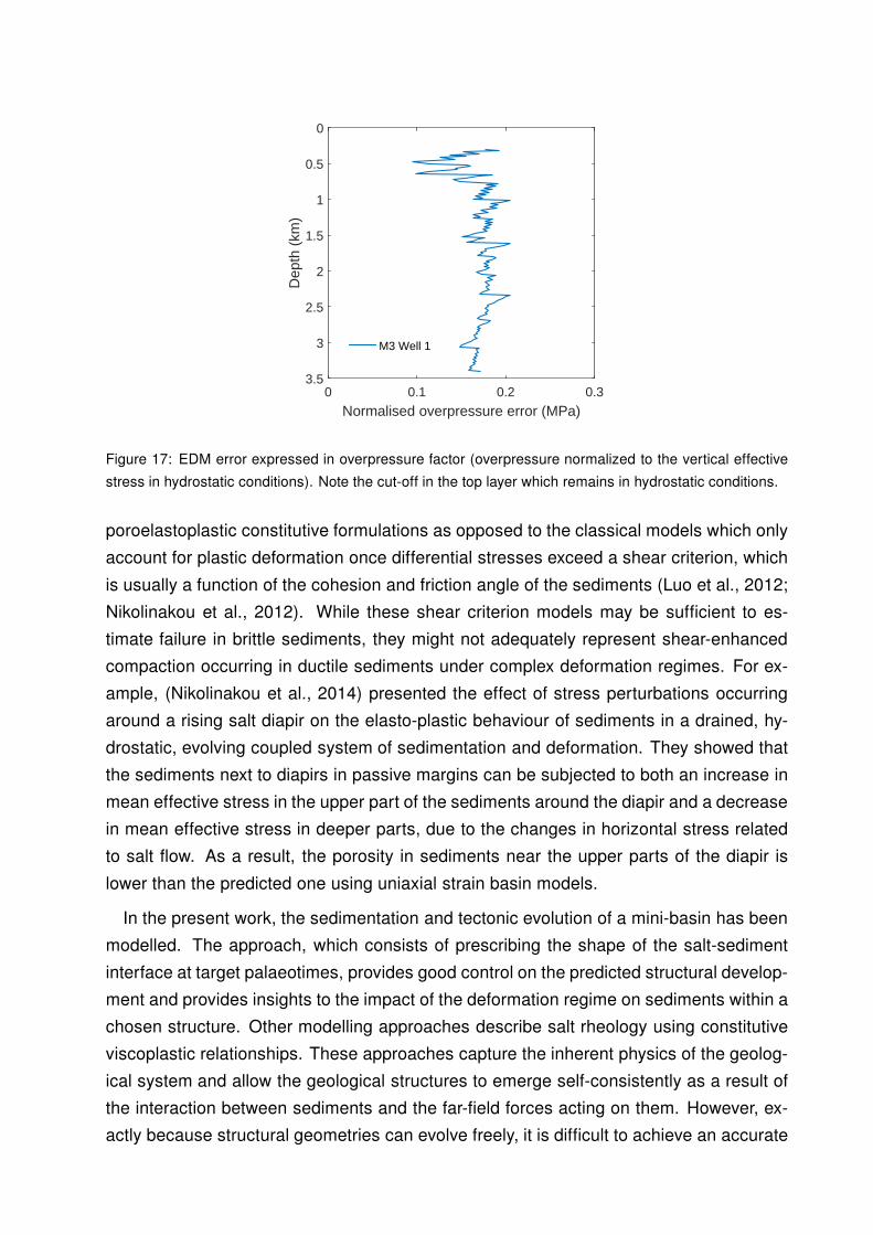
noted that the error in overpressure predicted by EDM increases with depth. In Fig. 17

the EDM error is expressed in terms of the overpressure factor, that is the overpressure

normalized to the maximum VES at each depth in hydrostatic conditions. The results

show an average normalized error of 0.17 in M3.

Porosity0.2 0.3 0.4 0.5

Dep

th (

km)

0

0.5

1

1.5

2

2.5

3

NCTM4 Well 1M3 Well 1M5

Overpressure (kPa)0 5 10 15 20 25

Dep

th (

km)

0

0.5

1

1.5

2

2.5

3

M4 Well 1 M3 Well 1EDM M4 Well 1EDM M3 Well 1

(a) (b)

Porosity0.3 0.4 0.5

Dep

th (

km)

0

0.5

1

1.5

NCTM4 Well 1 M3 Well 1M5

Overpressure (kPa)0 5 10 15

Dep

th (

km)

0

0.5

1

1.5

M4 Well 2M3 Well 2EDM M4 Well 2EDM M3 Well 3

(c) (d)

Figure 15: Porosity trends above the top sand layer for M3, M4 and M5 compared to clay NCT at (a) Well

1 and (c) Well 2. Finite element model overpressure comparison with equivalent depth method (EDM)

predicted overpressure for M3 and M4 at (b) Well 1 and (d) Well 2.

At Well 2 the porosities for M3 are lower than porosities for M5 because of the ver-

tical compaction caused by the diapir uplift in the former model; in contrast, in M4

the high overpressures transferred to this location lead to porosity preservation in the

subsequently-deposited sediments (Fig. 15c). EDM result in an underestimation of pore

pressure of up to 3 MPa at 1900 m depth in both models. Despite the deformation regime

Porosity0 0.2 0.4 0.6

Ver

tical

effe

ctiv

e st

ress

(M

Pa)

0

2

4

6

8

10

12

14

1D compactionM4 Well 1M3 Well 1

Effective stress ratio 0 0.5 1 1.5 2

Dep

th (

km)

0

0.5

1

1.5

2

2.5

3

3.5

M4 Well 1M3 Well 1

(b)(a)

Figure 16: Predictions at Well 1 for M3 and M4: (a) Effective stress ratio with depth and (b) porosity-VES

relationship. It is noted that the M3 porosity-VES curve is further from the 1D compaction than the M4

curve. This is due to the relatively higher contribution of lateral stress in M3 than in M4.

being laterally extensional at this location and the principal stress being vertical, some of

the compaction and overpressure generation is a consequence of the vertical tectonic

deformation. This results in deviations from the porosity-VES relationship assumed in 1D

models and overpressure predictions by EDM which are low relative to the true overpres-

sure magnitudes. It should be noted that, despite the overpressure increase by lateral

transfer at this location in M4, this does not result in additional error in EDM predic-

tions. The reason is that the tilting of the reservoirs was synchronous to deposition of

the overlaying clay. Consequently, the large overpressures hindered vertical compaction

with consequent porosity preservation. Thus, the additional overpressure transferred to

the anticlinal location is in agreement with the porosity-VES relationship. Therefore, lat-

eral transfer results in no additional deviation from the 1D compaction assumptions. A

completely different scenario would have occurred if the tectonic episode had started

after most or all sediments had been deposited. In this case the tectonically-induced

overpressure transferred from Well 1 to Well 2 would elastically unload the clay units,

resulting in an additional error in pore pressure estimated by the EDM.

6. Discussion

This paper has explored the impact of complex deformation regimes in a salt mini-

basin, and in particular overpressure generation, using a fully-coupled geomechanical-

fluid flow finite element model that employs a full 3D stress tensor together with an ad-

vanced constitutive model to describe the rheological behaviour of different lithologies.

Previous work has highlighted the benefits and the main differences of using advanced

Normalised overpressure error (MPa)0 0.1 0.2 0.3

Dep

th (

km)

0

0.5

1

1.5

2

2.5

3

3.5

M3 Well 1

Figure 17: EDM error expressed in overpressure factor (overpressure normalized to the vertical effective

stress in hydrostatic conditions). Note the cut-off in the top layer which remains in hydrostatic conditions.

poroelastoplastic constitutive formulations as opposed to the classical models which only

account for plastic deformation once differential stresses exceed a shear criterion, which

is usually a function of the cohesion and friction angle of the sediments (Luo et al., 2012;

Nikolinakou et al., 2012). While these shear criterion models may be sufficient to es-

timate failure in brittle sediments, they might not adequately represent shear-enhanced

compaction occurring in ductile sediments under complex deformation regimes. For ex-

ample, (Nikolinakou et al., 2014) presented the effect of stress perturbations occurring

around a rising salt diapir on the elasto-plastic behaviour of sediments in a drained, hy-

drostatic, evolving coupled system of sedimentation and deformation. They showed that

the sediments next to diapirs in passive margins can be subjected to both an increase in

mean effective stress in the upper part of the sediments around the diapir and a decrease

in mean effective stress in deeper parts, due to the changes in horizontal stress related

to salt flow. As a result, the porosity in sediments near the upper parts of the diapir is

lower than the predicted one using uniaxial strain basin models.

In the present work, the sedimentation and tectonic evolution of a mini-basin has been

modelled. The approach, which consists of prescribing the shape of the salt-sediment

interface at target palaeotimes, provides good control on the predicted structural develop-

ment and provides insights to the impact of the deformation regime on sediments within a

chosen structure. Other modelling approaches describe salt rheology using constitutive

viscoplastic relationships. These approaches capture the inherent physics of the geolog-

ical system and allow the geological structures to emerge self-consistently as a result of

the interaction between sediments and the far-field forces acting on them. However, ex-

actly because structural geometries can evolve freely, it is difficult to achieve an accurate

representation of the actual geometry, with onward implications for predicting present-day

pore pressures. The methodology presented here is therefore advantageous in circum-

stances where the goal is to model a specific field area, especially when depth-converted

seismic cross sections and structural restorations are available for model calibration. By

using a depth-converted seismic cross section to prescribe the present day salt-sediment

interface for a base case model, the assumed salt-sediment shape at target palaeotimes

has enabled the reproduction of structural features observed in the field such as the syn-

clinal shape of the depocentres, the onlapping of sediments on salt and the anticlinal

folding due to the rise of a salt diapir.

Furthermore, the adopted approach allows us to impose lateral shortening of sedi-

ments, which in turn enables the quantitative demonstration that classical approaches

which rely on 1D compaction assumptions are unlikely to provide accurate predictions of

pore pressure in regions subjected to recent tectonic activity. The analysis shows that

classical pore pressure prediction methods not only fail to capture the compaction and

overpressure state in sediments undergoing lateral tectonic compaction, but also in those

areas subjected to vertical tectonic compaction.

The presented models capture the deposition of sediments, the vertical mechanical

compaction due to the vertical effective stress exerted by the weight of the overlying sed-

iments, the vertical and lateral mechanical compaction due to the increase in effective

stresses induced by the tectonic deformation, the overpressure generation due to me-

chanical compaction and fluid flow. Sedimentation rates in the target mini-basins are fast

(2000 m/Ma) and the sediments are young (Pliocene-Pleistocene to present) and often

poorly consolidated. Consequently, the assumption of neglecting chemical compaction is

reasonable provided that the hardening law for the sediments is calibrated to field rather

than experimental observations. This ensures that realistic porosities are predicted, es-

sential to a coupled geomechanical/fluid flow analysis. In this case the hardening law of

the sediments (which has a first order effect on mechanical compaction) has been cali-

brated according to a regional compaction trend for Golf of Mexico published in (Hudec

et al., 2009).

7. Conclusion

From the fully coupled geomechanical and fluid flow analysis performed within this

work we conclude that:

• The boundary-driven approach used in this paper has enabled a base case, present-

day geometry and structural configuration to be constrained using a depth-converted,

uninterpreted seismic cross section and a schematic of the geometry of the Titan

mini-basin. It has also facilitated the introduction of lateral shortening within the

models, with control on the final salt-sediment interface. Imposing 20% of horizon-

tal shortening synchronous to sedimentation increased the effective stress ratios in

the laterally compressive depocentres and decreased them in the anticlinal, later-

ally extensile location. Overpressure increased up to 10 MPa in the left depocentre

(26% of the total overpressure) with relatively small differences in porosity.

• The rise of the central salt diapir resulting from the imposed deformation regime

caused vertical tectonic compaction of overlying sediments with a consequent pore

pressure increase and porosity decrease. This is not captured in 1D compaction

models.

• Porosity-based pore pressure predictions based on 1D compaction models are not

suitable in regions with recent tectonic activity. The error in overpressure magnitude

resulting from EDM predictions in the analysed cases is up to 6 MPa at 3.4 km

depth (the average difference is 17% of the maximum vertical effective stress in

hydrostatic conditions at each depth).

• In the cases studied here, lateral transfer of fluid pressure has decreased the error

resulting from EDM predictions in the compressional depocentres, whereas it has

shown to have no impact in the location of the laterally extensional anticline.

Acknowledgements The authors would like to acknowledge the sponsors BG Group,

BP, Chevron, ConocoPhillips, DONG Energy, E.ON, ENI, Petrobras, Petronas, Statoil,

Total and Tullow Oil of the GeoPOP3 (Geosciences Project on OverPressure) project for

the financial support. We thank Neil Goulty, Vania Orozova-Bekkevold and the anony-

mous reviewers for their valuable comments which helped improve the paper.

References

Albertz, M., Lingrey, S., 2012. Critical statefinite element models of contractional fault-

related folding: Part 1. structural analysis. Tectonophysics 576-577, 133–149.

Biot, M. A., 1941. General theory of three-dimensional consolidation. J. Appl. Phys. 12,

155–164.

Biot, M. A., 1955. Theory of elasticity and consolidation for a porous anisotropic solid. J.

Appl. Phys. 26, 182–185.

Biot, M. A., Willis, D. G., 1957. The elastic coefficients of the theory of consolidation. J.

Appl. Phys. 24, 594–601.

Brun, J. P., Fort, X., 2004. Compressional salt tectonics (angolan margin). Tectono-

physics 382 (3-4), 129–150.

Cacas-Stenz, M. C., Arbeaumont, A., Faille, I., 2015. A new method to take lateral stress

into account in petroleum system simulation. In: Geopressure 2015: The life history of

a well, 14-16 April, Durham, UK.

Couzens-Schultz, B. A., Azbel, K., 2014. Predicting pore pressure in active fold-thrust

systems: An empirical model for the deepwater sabah foldbelt. Journal of Structural

Geology 69, 465–480.

Crook, A., Willson, S., Yu, J., Owen, D., 2006. Predictive modelling of structure evolution

in sandbox experiments. Journal of Structural Geology 28 (5), 729–744.

Crook, A. J. L., 2013. ParaGeo: A Finite element model for coupled simulation of the

evolution of geological structures. Three Cliffs Geomechanical Analysis, Swansea, UK.

Dean, R., Gai, X., Stone, C., Minkoff, S., 2003. A comparison of techniques for coupling

porous flow and geomechanics. SPE Journal 11 (1), 132–140.

Desai, C., Salami, M., 1987. A constitutive model and associated testing for soft rock. Int.

J. Rock Mech. Min. Sci. 24, 299–307.

Flemings, P., Lupa, J., 2004. Pressure prediction in the bullwinkle basin through petro-

physics and flow modeling (green canyon 65, gulf of mexico). Marine and Petroleum

Geology 21 (10), 1311–1322.

Hantschel, T., Kauerauf, A., 2009. Fundamentals of Basin and Petroleum Systems Mod-

eling, berlin Edition. Springer-Verlag.

Hubbert, M. K., Rubey, W. W., 1959. Role of fluid pressure in mechanics of overthrust

faulting. Geological Society of America Bulletin 70 (2), 115–166.

Hudec, M. R., Jackson, P. A., Schultz-Ela, D. D., 2009. The paradox of minibasin subsi-

dence into salt: Clues to the evoltuion of crustal basins. Geological Society of America

Bulletin 121 (1/2), 201–221.

Jackson, P. A., Talbot, C. J., 1986. External shapes,strain rates, and dynamics of salt

structures. Geological Society of America Bulletin 97 (3), 305–323.

Jha, B., Juanes, R., 2007. A locally conservative finite element framework for the simu-

lation of coupled flow and reservoir geomechanics. Acta Geotechnica 2 (3), 139–153.

Kane, I., McGee, D., Jobe, Z., 2012. Halokinetic effects on submarine channel equilib-

rium profiles and implications for facies architecture: conceptual model illustrated with

a case study from magnolia field, gulf of mexico. Geological Society. Special Publica-

tions 363 (3), 289–302.

Kjeldstad, A., Skogseid, J., Langtangen, H. P., Bjørlykke, K., Høeg, K., 2003. Differential

loading by prograding sedimentary wedges on continental margins: An arch-forming

mechanism. J. Geophys. Res. 108 (B1-2036).

Lewis, R. W., Schrefler, B. A., 1998. The finite element method in the static and dynamic

deformation and consolidation of porous media. Wiley.

Lewis, R. W., Sukirman, Y., 1993. Finite-element modeling of three-phase flow in de-

forming saturated oil-reservoirs. Int. J. for Num. and Anal. Meth. Geomech. 17 (8),

577–598.

Luo, G., Nikolinakou, M., Flemings, P., Hudec, M., 2012. Geomechanical modeling of

stresses adjacent to salt bodies: Part 1 - uncoupled models. AAPG Bulletin 96 (1),

43–64.

Maghous, S., Bruch, A., Bernaud, D., Dormieux, L., Braun, A. L., 2014. Two-dimensional

finite element analysis of gravitational and lateral driven deformation in sedimentary

basins. Int. J. for Num. and Anal. Meth. Geomech. 38, 725–746.

Mainguy, M., Longuemare, P., 2002. Coupling fluid flow and rock mechanics: formula-

tions of the partial coupling between reservoir and geomechanics simulators. Oil Gas

Sci. Technol. 57, 355–367.

Marton, L. G., Tari, G. C., Lehmann, C. T., 2000. Evolution of the angolan passive margin,

west africa, with emphasis on postsalt structural styles. American Geophysical Union,

Geophysical Monograph Series 115, 129–149.

Neumaier, M., Littke, R., Hantschel, T., Maerten, L., Joonnekindt, J. P., Kukla, P., 2014.

Integrated charge and seal assesment in the monagas fold and thrust belt of venezuela.

AAPG Bulletin 98 (7), 1325–1350.

Nikolinakou, M. A., Flemings, P. B., Hudec, M. R., 2014. Modeling stress evolution around

a rising salt diapir. Marine and Petroleum Geology 51, 230–238.

Nikolinakou, M. A., Luo, G., Hudec, R., M., Flemings, P. B., 2012. Geomechanical mod-

eling of stresses adjacent to salt bodies: Part 2 - poroelastoplasticity and coupled

overpressures. AAPG Bulletin 96 (1), 65–85.

Settari, A., Mourits, F. M., 1998. A coupled reservoir and geomechanical simulation sys-

tem. SPE Journal 3 (03), 219–226.

Settari, A., Walters, D. A., 2001. Advances in coupled geomechanical and reservoir mod-

elling with applications to reservoir compaction. SPE Journal 6 (03), 334–342.

Smart, K. J., Ferrill, D. A., Morris, A. P., McGinnis, R. N., 2012. Geomechanical modeling

of stress and strain evolution during contractional fault-related folding. Tectonophysics

576-577, 171–196.

Soleymani, H., Riahi, M., 2012. Velocity based pore pressure prediction - a case study at

one of the iranian southwest oil fields. Journal of Petroleum Science and Engineering

94-95 (9), 40–46.

Styzen, M. J., 1996. A chart in two sheets of the late cenozoic chronostratigraphy of the

gulf of mexico,gulf coast section. In: AAPG annual convention, May 11-14, Salt Lake

City, Utah. Gulf Coast Section of SEPM Foundation Publication.

Swarbrick, R. E., 2002. Challenges of porosity-based pore pressure prediction. CSEG

Recorder, 75–78.

Terzaghi, K. v., 1923. Die berchnung der durchassigkeitziffer des tones aus dem ver-

lauf der hydrodynamischen spannungscheinungen. Sitzunzsber Akad Wiss. Wein Math

Naturwiss IIa (3-4), 125–138.

Thomas, L. K., Chin, L. Y., Pierson, R. G., Sylte, J. E., 2002. Coupled geomechanical

and reservoir simulation. In: SPE Annual Technical Conference and Exhibition, 29

September - 2 October, San Antonio, Texas. Gulf Coast Section of SEPM Foundation

Publication.

Thornton, D. A., Crook, A. J. L., 2014. Predictive modelling of the evolution of fault struc-

ture: 3-d modelling and coupled geomechanical/flow simulation. Rock Mechanics and

Rock Engineering 47 (5), 1533–1549.

Tran, D., Settari, A., Nghiem, L., 2004. New iterative coupling between reservoir simulator

and geomechanics module. SPE Journal 9 (03), 362–369.

Wood, D. M., 1990. Soil Behaviour and Critical State Soil Mechanics. Cambridge Univer-

sity Press.

Yang, Y., Aplin, A. C., 2004. Definition and practical application of mudstone porosity-

effective stress relationships. Petroleum Geoscience 10, 153–162.

Yang, Y., Aplin, A. C., 2010. A permeability-porosity relationship for mudstones. Marine

and Petroleum Geology 27 (8), 1692–1697.

Yardley, G. S., Swarbrick, R. E., 2000. Lateral transfer: a source of additional overpres-

sure? Mar. Pet. Geol 17 (4), 523–537.

Zhang, J., 2011. Pore pressure prediction from well logs: Methods, modifications, and

new approaches. Earth-Science Reviews 108 (1-2), 50–63.

Zhang, J., 2013. Effective stress, porosity, velocity and abnormal pore pressure prediction

accounting for compaction disequilibrium and unloading. Mar. Pet. Geol. 45 (8), 2–11.

AppendixA. SR4 Constitutive model

A three-invariant rate-independent poro-elastic-plastic critical state constitutive model

with non-associative plasticity is adopted in this study. The yield surface delimitates the

domain of stress states that produce elastic and elastic-plastic strains. Stress states

inside the yield surface produce elastic deformation whereas stress states that belong to

the yield surface produce elastic-plastic deformation. Poro-elastic deformations rely on

the existence of a non-linear porosity and stress state dependent function:

Kb = Kb0 + (1− Aun)pc

κ+ Aun

p′

(1− φ)κ(AppendixA.1)

whereKb is the bulk modulus, pc is the pre-consolidation pressure, p′ is the mean effective

stress. Kb0 is the bulk modulus at deposition (i.e. when pc → 0 and p′ → 0), κ is the elastic

unloading modulus and Aun is the dependence factor which have values 0 ≤ Aun ≤ 1.

Note that when Aun = 1 the poro-elastic law is identical to that of the Modified Cam-Clay

model (MCC). In the present work the parameter has been adjusted to Aun = 0.5.

The yield surface in the deviatoric plane (plane normal to hydrostatic axis) is computed

as:

g(θ, p′) =

[

1

1− βπ(p′)

(

1 + βπ(p′) sin(3θ))

]Nπ

(AppendixA.2)

where Nπ is a deviatoric plane shape material constant and βπ(p′) is a function defined

as (Desai and Salami, 1987):

βπ(p′) = βπ0 exp

(

βπ1 p′pc0

pc

)

(AppendixA.3)

where βπ0 and βπ1 are material constants and pc0 is the initial pre-consolidation pressure

(corresponding to uncompressed and undamaged material).

Compaction and dilation regions of the plastic domain are divided by the critical state

line. Stress states that reach the current yield surface on the compression domain will

cause a diffuse volumetric plastic strain and an increase in both, pre-consolidation pres-

sure and yield surface size (strength increase or hardening) whereas stress states that

reach the yield surface on the dilation domain will cause a shear localization with vol-

ume increase and a decrease in both, pre-consolidation pressure and yield surface size

(strength decrease or softening). Continuous shearing in a stress state corresponding to

the intersection of the critical state line and the yield surface induces continuous shear

plastic strain at constant volume. The hardening and softening of materials with the

corresponding evolution of the yield surface is controlled by the hardening law which is

defined as a function of the plastic volumetric strain:

pc(εpv) = pc0 exp

[

−v(εpv)

(λ− κ)

]

(AppendixA.4)

and

pt(εpv) = pt0 exp

[

−v(εpv)max(λ− κ)

]

(AppendixA.5)

where v is the specific volume and v = 1 + e, e is the void ratio, λ and κ are the slopes

of the normal compression line (NCL) and unloading-reloading line in the e − ln p′ plane

and (εpv)max is the maximum dilatational volumetric plastic strain.

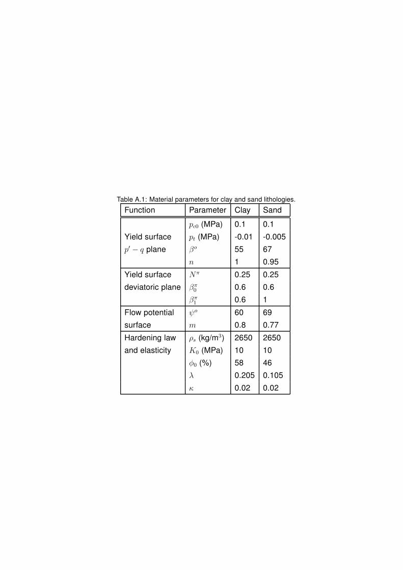
AppendixA.1. Material properties

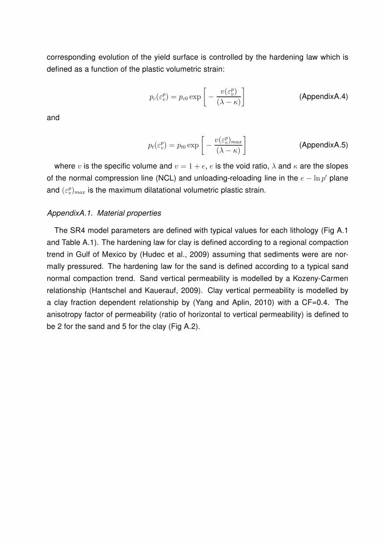
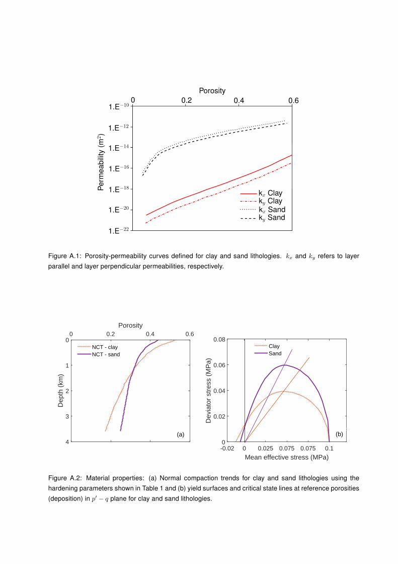
The SR4 model parameters are defined with typical values for each lithology (Fig A.1

and Table A.1). The hardening law for clay is defined according to a regional compaction

trend in Gulf of Mexico by (Hudec et al., 2009) assuming that sediments were are nor-

mally pressured. The hardening law for the sand is defined according to a typical sand

normal compaction trend. Sand vertical permeability is modelled by a Kozeny-Carmen

relationship (Hantschel and Kauerauf, 2009). Clay vertical permeability is modelled by

a clay fraction dependent relationship by (Yang and Aplin, 2010) with a CF=0.4. The

anisotropy factor of permeability (ratio of horizontal to vertical permeability) is defined to

be 2 for the sand and 5 for the clay (Fig A.2).

Porosity

0 0.2 0.4 0.6

ky Clay

ky Sandkx Sand

kx Clay

1.E−10

1.E−12

1.E−14

1.E−16

1.E−18

1.E−20

1.E−22

Pe

rme

ab

ility

(m2)

Figure A.1: Porosity-permeability curves defined for clay and sand lithologies. kx and ky refers to layer

parallel and layer perpendicular permeabilities, respectively.

Porosity0 0.2 0.4 0.6

Dep

th (

km)

0

1

2

3

4

NCT - clayNCT - sand

Mean effective stress (MPa)-0.02 0 0.025 0.075 0.075 0.1

Dev

iato

r st

ress

(M

Pa)

0

0.02

0.04

0.06

0.08ClaySand

(b)(a)

Figure A.2: Material properties: (a) Normal compaction trends for clay and sand lithologies using the

hardening parameters shown in Table 1 and (b) yield surfaces and critical state lines at reference porosities

(deposition) in p′ − q plane for clay and sand lithologies.

Table A.1: Material parameters for clay and sand lithologies.

Function Parameter Clay Sand

pc0 (MPa) 0.1 0.1

Yield surface pt (MPa) -0.01 -0.005

p′ − q plane βo 55 67

n 1 0.95

Yield surface Nπ 0.25 0.25

deviatoric plane βπ0 0.6 0.6

βπ1 0.6 1

Flow potential ψo 60 69

surface m 0.8 0.77

Hardening law ρs (kg/m3) 2650 2650

and elasticity K0 (MPa) 10 10

φ0 (%) 58 46

λ 0.205 0.105

κ 0.02 0.02

List of Figures

1 Definition of initial and present day geometry boundaries using an uninter-

preted seismic cross section of the Titan mini-basin (Kane et al., 2012). . 6

2 Geometry boundaries at times t=5 Ma b.p. (initial time) and 1.4 Ma b.p.

for Models M1 to M4 and comparison of present day geometry boundary

for Models M1 and M2 and present day geometry boundary for Models M3

and M4. . . . . . . . . . . . . . . . . . . . . . . . . . . . . . . . . . . . . . 7

3 SR4 constitutive model (a) Yield and flow surfaces in the p′ − q plane and

(b) Yield surface in the deviatoric plane. . . . . . . . . . . . . . . . . . . . 10

4 Schematic representation of the sedimentation process. A mini-basin is

depicted at three different times within the deposition period of layer 2.

For the sake of simplicity the shape of the salt-sediment interface is kept

unchanged in the diagrams and the depositional surfaces are depicted as

horizontal surfaces. d∗: prescribed displacement, t0: initial time of the

depositional period of layer 2, tf : final time of the depositional period of

layer 2 and initial time of the depositional period of layer 3, t: current time,

SH: sedimentation horizon. (a) A new mesh is created for layer 2 with its

geometry delimited by the SH, the salt-sediment interface and the top of

layer 1. (b) Gravity on layer 2 is applied gradually and linearly to simulate

continuous deposition. Layer 2 is in hydrostatic conditions and the outflow

boundary is located on top of layer 2. (c) Layer 2 is completely deposited

and the hydrostatic constraint is removed in this layer. Outflow boundary

is located at top of layer 2. Start of the depositional period for layer 3. . . 13

5 Basin geometry for Models M1 and M2 at 2 Ma b.p., 1 Ma b.p. and the

present day. Stratigraphy is coloured from blue for the oldest layer to red

to the youngest one. . . . . . . . . . . . . . . . . . . . . . . . . . . . . . . 14

6 Effective stress ratio contour plots at present day for (a) Model M2 and (b)

Model M4. . . . . . . . . . . . . . . . . . . . . . . . . . . . . . . . . . . . . 14

7 Model M4: (a) Horizontal strain and (b) vertical strain. Positive values

indicate extension whereas negative values correspond to compression.

The two depocentres experience horizontal compression due to the lateral

shortening (a). The sediments above the central salt diapir experience

lateral extension and additional vertical compression due to the complex

deformation regime produced by the anticlinal folding and uplift promoted

by the rise of the salt. . . . . . . . . . . . . . . . . . . . . . . . . . . . . . 15

8 Model M4: Minimum principal effective stress contours. The minimum

principal effective stress is the difference between the principal effective

stress and the pore pressure and therefore is indicative of the drilling window. 16

9 Mohr circles for the clay overlying the reservoirs in the central anticline for

(a) Model M2 and (b) Model M4. . . . . . . . . . . . . . . . . . . . . . . . 17

10 Overpressure contours at present day with notional wells 1 and 2 locations

for (a) Model M1, (b) Model M3 and (c) Model M4. Colour scale shows the

full range of overpressure values for each model. . . . . . . . . . . . . . . 18

11 Overpressure profiles with depth comparison for models M1, M3 and M5

at (a) Well 1 and (b) Well 2. . . . . . . . . . . . . . . . . . . . . . . . . . . 19

12 Fluid flow directions nearby the anticline above the central salt diapir. Note

the sub-parallel layer bedding flow in the oldest layers, contributing to the

overpressure distribution from compressive to extensive regions. . . . . . 20

13 Overpressure profiles with depth comparison for models M3 and M4 at (a)

Well 1 and (b) Well 2 showing the impact of lateral transfer. . . . . . . . . 21

14 Porosity contour plots for models (a) M3 and (b) M4. Both models are

plotted using the same scale (which is covers the full range of porosity for

M4) to facilitate the comparison. In M3 the lowest porosity predicted was

0.2. . . . . . . . . . . . . . . . . . . . . . . . . . . . . . . . . . . . . . . . 22

15 Porosity trends above the top sand layer for M3, M4 and M5 compared to

clay NCT at (a) Well 1 and (c) Well 2. Finite element model overpressure

comparison with equivalent depth method (EDM) predicted overpressure

for M3 and M4 at (b) Well 1 and (d) Well 2. . . . . . . . . . . . . . . . . . 23

16 Predictions at Well 1 for M3 and M4: (a) Effective stress ratio with depth

and (b) porosity-VES relationship. It is noted that the M3 porosity-VES

curve is further from the 1D compaction than the M4 curve. This is due to

the relatively higher contribution of lateral stress in M3 than in M4. . . . . 24

17 EDM error expressed in overpressure factor (overpressure normalized to

the vertical effective stress in hydrostatic conditions). Note the cut-off in

the top layer which remains in hydrostatic conditions. . . . . . . . . . . . . 25

A.1 Porosity-permeability curves defined for clay and sand lithologies. kx and

ky refers to layer parallel and layer perpendicular permeabilities, respectively. 34

A.2 Material properties: (a) Normal compaction trends for clay and sand litholo-

gies using the hardening parameters shown in Table 1 and (b) yield sur-

faces and critical state lines at reference porosities (deposition) in p′ − q

plane for clay and sand lithologies. . . . . . . . . . . . . . . . . . . . . . . 34

List of Tables

1 List of the numerical models. . . . . . . . . . . . . . . . . . . . . . . . . . 4

2 Layer discretisation and depositional sequence. ∗Clay in single lithology

Models M1, M3 and M5. . . . . . . . . . . . . . . . . . . . . . . . . . . . . 5

A.1 Material parameters for clay and sand lithologies. . . . . . . . . . . . . . . 35