Observations on Business Cycle Accounting ∗ Lawrence J. Christiano † Joshua M. Davis ‡ December, 2005. Abstract Chari, Kehoe and McGrattan (2005) advocate the use of business cycle account- ing to identify directions for improvement in equilibrium business cycle models. This procedure computes the ‘wedges’ in a first-generation RBC model that are necessary for the model to reproduce major macroeconomic time series. As a demonstration of the power of the approach, CKM argue that it can be used to rule out a prominent class of explanations of the Great Depression. In particular, they conclude that models of financial frictions which create wedges in the intertemporal Euler equation are not promising avenues for understanding the dynamics of the Great Depression. We have two main findings. First, when we modify the RBC model to include in- vestment adjustment costs, we find that the CKM results are overturned: shocks in the intertemporal Euler equation account for a significant fraction (25-40 percent) of the fall in output in the Great Depression. Second, we show that the use of business cy- cle accounting to determine the importance of intertemporal Euler equation shocks in output dynamics depends on identification assumptions. But, there are many observa- tionally equivalent assumptions that one can make, and each has different implications for the importance of intertemporal Euler equation errors. ∗ The first authors is grateful for the financial support of a National Science Foundation grant. † Northwestern University, National Bureau of Economic Research. ‡ Northwestern University, National Bureau of Economic Research, and Federal Reserve Bank of Chicago.
Transcript
Observations on Business Cycle Accounting∗
Lawrence J. Christiano† Joshua M. Davis‡
December, 2005.
Abstract
Chari, Kehoe and McGrattan (2005) advocate the use of business cycle account-ing to identify directions for improvement in equilibrium business cycle models. Thisprocedure computes the ‘wedges’ in a first-generation RBC model that are necessaryfor the model to reproduce major macroeconomic time series. As a demonstration ofthe power of the approach, CKM argue that it can be used to rule out a prominentclass of explanations of the Great Depression. In particular, they conclude that modelsof financial frictions which create wedges in the intertemporal Euler equation are notpromising avenues for understanding the dynamics of the Great Depression.We have two main findings. First, when we modify the RBC model to include in-
vestment adjustment costs, we find that the CKM results are overturned: shocks in theintertemporal Euler equation account for a significant fraction (25-40 percent) of thefall in output in the Great Depression. Second, we show that the use of business cy-cle accounting to determine the importance of intertemporal Euler equation shocks inoutput dynamics depends on identification assumptions. But, there are many observa-tionally equivalent assumptions that one can make, and each has different implicationsfor the importance of intertemporal Euler equation errors.
∗The first authors is grateful for the financial support of a National Science Foundation grant.†Northwestern University, National Bureau of Economic Research.‡Northwestern University, National Bureau of Economic Research, and Federal Reserve Bank of Chicago.
1. Introduction
Chari, Kehoe and McGrattan (2005) (CKM) argue that a procedure they call Business CycleAccounting (BCA) is useful for identifying promising directions for model development.1 Thestrategy works with the first-generation real business cycle (RBC) model as a benchmark. Itisolates the wedges between marginal rates of substitution in preferences and marginal ratesof substitution in technology necessary for the model to be able to reproduce key macro-economic aggregates. Under BCA, the parts of the model that deserve further developmentare the ones with the most important wedges. After applying their methodology to the USGreat Depression, CKM reach a surprising conclusion. Financial frictions of the sort thatmanifest themselves primarily in the intertemporal wedge (the one between the intertem-poral marginal rate of substitution in consumption and the rate of return on capital) arenot useful for thinking about the US Great Depression. This appears to rule out models offinancial frictions like those analyzed by Carlstrom and Fuerst (1997) (CF) and Bernanke,Gertler and Gilchrist (1999) (BGG).We make two observations. First, we focus on the assumption in CKM’s benchmark RBC
model, that the technology for producing new capital is linear in investment and old capital.We find that when we introduce curvature (‘adjustment costs’) into this relationship, theCKM conclusion is overturned.2 Second, we show that the use of BCA to identify the mostimportant wedges is hampered by a fundamental identification problem. Determining theimportance of a wedge in model dynamics requires making identification assumptions, butthe framework offers no way to evaluate alternative assumptions.We now discuss our two findings in greater detail. We document the importance of
curvature by introducing adjustment costs into CKM’s benchmark model and redoing theirwedge calculations. We choose the degree of adjustment costs by calibrating the model’simplication for the Tobin’s q elasticity, that is, the elasticity of the investment to capital ratiowith respect to the price of capital. To be conservative, we adopt the smallest adjustmentcost consistent with the empirical evidence on Tobin’s q reported in Abel (1980) and Eberly(1997). When we apply BCA using the modified RBC model, we find that financial frictionswhich enter primarily through the intertemporal wedge account for 25-40 percent of the fallof output during the Great Depression. The reason CKM’s findings are not robust to thepresence of adjustment costs is that adjustment costs and the intertemporal wedge in effectcancel each other, when viewed from the perspective of the first-generation RBC model.3
Leave out adjustment costs and there is no apparent need for an intertemporal wedge. Theintuition for this is simple.The rate of return on capital - measured in the way that is consistent with the standard
RBC model - falls at roughly the same rate as does consumption growth during the first
1This strategy is closely related to that advocated in Parkin (1988), Ingram, Kocherlakota and Savin(1994), Hall (1997), and Mulligan (2002).
2In considering robustness to perturbations in their analysis, CKM also consider adjustment costs ininvestment. In contrast to our findings, they report that their results are robust to the introduction ofadjustment costs. Their paper does not provide enough information for us to assess the reason for thedifferent results. For example, CKM do not report the numerical value of the parameter of their adjustmentcost function.
3We are grateful to Mark Gertler, who conjectured this result in a private communication.
2
years of the Great Depression. Equality of the intertemporal marginal rate of substitutionin consumption, MRS, and rate of return on capital, 1 + Rk, occurs without the need of awedge between the two. In particular,
MRS ≈ 1 +Rk,
during the first few years of the Great Depression, when Rk is measured as in the first-generation RBC model.4 When adjustment costs are introduced, a capital gain term appearsin the rate of return on capital. The modified model associates the collapse in output andinvestment at the start of the Great Depression with a low value of the price of capital.Because of the stationarity properties of the RBC model, the price of capital is expected torise back up to its steady state value. This anticipated capital gain implies that Rk actuallyrises in the first few years of the Great Depression. Now a wedge, 1− τk, is required to bringMRS and 1 +Rk into line:
MRS =¡1− τk
¢ ¡1 +Rk
¢.
The intertemporal wedge, 1− τk, must fall with the rise in Rk.5
We now briefly describe our point about lack of identification in BCA. In modeling thewedges, a flexible time series representation is adopted in which the dynamic and contempo-raneous interactions between wedges is left unrestricted. This is very much in the spirit ofthe analysis, because most extensions of the first generation RBC models do imply that thewedges are correlated. A shock that originates inside one wedge moves all other wedges.6
Our identification point can be understood by contemplating closely the sort of questionthat BCA is designed to answer: ‘what is the contribution to aggregate fluctuations of thesort of financial frictions that manifest themselves in the form of intertemporal wedges?’ Thisquestion can be interpreted in at least two ways: (i) ‘what is the role of financial frictions, asa source of macroeconomic impulses?’ For example, when the financial frictions studied byCF or BGG are introduced, one can contemplate new shocks, such as shocks to monitoringcosts, or to the riskiness of entrepreneurs.7 Another interpretation is (ii), ‘what is the roleof financial frictions as a propagation mechanism for traditional macroeconomic impulses?’Answering (ii) requires comparing the actual effects of non-financial friction shocks with whattheir effects are when financial frictions are shut down. But, given the lack of structure inBCA, there is no hope of addressing this question. We take it for granted that BCA cannotaddress question (ii). We argue that underidentification also mars the ability to address (i).
4In this case, 1 +Rk =MPk + (1− δ) , where MPk is the marginal physical product of capital.5Primiceri, Schaumburg and Tambalotti (2005) make a related argument. They note that if one measures
Rk using a market return, then one finds that 1 − τk varies substantially in post-war data. Market basedmeasures of Rk exhibit orders of magnitude greater fluctuations than does Rk in the first-generation RBCmodel. This argument is related to the rejections of intertemporal Euler equations reported by Hansen andSingleton (1982,1983 ) and others.
6For example, with sticky wages and/or sticky prices the marginal rate of substitution between con-sumption and leisure is only equal to the marginal product of labor on average. A shock that enters theintertemporal Euler equation will in general have a different impact on the marginal rate of substitutionthan on the marginal product of labor. That is, it will move what CKM call the leisure wedge. This effectis expected to occur contemporaneously, and over time.
7Shocks like these are explored in the context of the Great Depression by Christiano, Rostagno and Motto(2004) and in the context of recent business cycles in the Euro Area and the US by Christiano, Rostagnoand Motto (2005).
3
The implicit identification assumption underlying CKM’s implementation of BCA is thatthe shocks originating in the intertemporal wedge are exclusively financial friction shocks,and that those shocks do not spill over into the other wedges. Identification is a substantialissue when, under CKM’s implicit identification assumptions, one finds that intertemporalwedges matter. This is the relevant case, because, as noted above, we find that the intertem-poral wedge matters when adjustment costs are included in the RBC model. The problem isthat one can interpret the estimated covariation among wedges as implying that much of themovement in the intertemporal wedge actually reflects shocks originating in other wedges. Inthis case, the 25-40 percent number we reported above is an overestimate of the importanceof shocks originating in the intertemporal wedge. Alternatively, one can interpret the co-variation among wedges as reflecting that shocks originating in the intertemporal wedge spillover into other wedges. In this case, our 25-40 percent estimate understates the importanceof shocks originating in the intertemporal wedge. To make this point concrete, we find anidentification which has the implication that shocks originating in the intertemporal wedgeaccount for 100% of the behavior of output, employment and investment during the GreatDepression. There is no way to select between the alternative identification assumptionsthat support these different conclusions about the importance of the shocks originating inthe intertemporal wedge. This is because each identification assumption is observationallyequivalent.In the following section, we describe the model used in the analysis. In section 3, we
discuss our model solution and estimation strategy. In section 4 we spell out the identificationproblem discussed above. In section 5 we discuss how the importance of a particular wedge isassessed, given a set of identification assumptions. Section 6 displays our results. Concludingremarks appear in section 7.
2. Model
According CKM’s first-generation RBC model, households maximize:
where ct and lt denote per capita consumption and employment, respectively. The householdbudget constraint is
ct + (1 + τx,t)xt ≤ rtkt + (1− τ l,t)wtlt + Tt,
where Tt denotes lump sum taxes, xt denotes investment and τ l,t denotes the labor wedge.Also, kt denotes the beginning-of-period t stock of capital divided by the period t popu-lation. As discussed in the introduction the intertemporal wedge, τx,t, is motivated usingthe CF model. In addition, the household satisfies the following accumulation equation forinvestment:
(1 + gn) kt+1 = (1− δ) kt + xt. (2.1)
The household maximizes utility by choice of kt+1, xt, ct and lt, subject to its budget con-straint, the capital evolution equation and the usual inequality constraints and no-Ponzischeme condition.
and Zt, the efficiency wedge, is an exogenous stationary stochastic process. In the resourceconstraint, Gt denotes government purchases of goods and services, which have the followingrepresentation:
gt = gt (1 + gz)t ,
where gt is a stationary, exogenous stochastic process and gz ≥ 0.Combining firm and household first order necessary conditions for optimization,
−ul,tuc,t
= (1− τ l,t) yl,t (2.3)
uc,t = βEtuc,t+1yk,t+1 + (1 + τx,t+1) (1− δ)
(1 + τx,t), (2.4)
where uc,t and −ul,t are the derivatives of period utility with respect to consumption andleisure, respectively. In addition, yl,t and yk,t are the marginal products of labor and capital,respectively. The solution to the model is obtained by solving (2.1)-(2.4) subject to thetransversality condition and the law of motion for the exogenous shocks. This is given by:
st = P0 + Pst−1 +Qεt, st =
⎛⎜⎜⎝log Zt
τ l,tτx,tlog gt
⎞⎟⎟⎠ , Eεtε0t = I, (2.5)
where
P =
∙P 00 p44
¸, Q =
∙Q 00 q44
¸.
Here, P is unrestricted and Q is normalized to be lower triangular with non-negative diago-nal terms. The shocks, εt, have no particular economic significance. The assumption abouttheir variance and cross-correlations, as well as the lower triangularity of Q are simply nor-malizations. In effect, the dynamic interaction between the first three wedges (i.e., elementsof st) is left unrestricted. Their statistical relationship to gt is sharply restricted. However,we did not find that the results in this note are very sensitive to this assumption, and so wedo not explore that more here.CKM also consider the case of adjustment costs in investment, a > 0. We consider the
model of adjustment costs used in CKM:
(1 + gn) kt+1 = (1− δ) kt + xt − Φ
µxtkt
¶kt, (2.6)
where
Φ
µxtkt
¶=
a
2
µxtkt− b
¶2. (2.7)
5
Here, b is the steady state investment to capital ratio.In Appendix A, we derive the equilibrium conditions for the CF model when the technol-
ogy for producing new capital is given by (2.6)-(2.7) with a > 0. We establish a propositiondisplaying the wedges that must be added to the RBC economy to ensure that the equilibriumallocations of the RBC economy coincide with those of the CF economy with adjustmentcosts. We show that the intertemporal wedge implied by the CF model has the followingform:
uc,t = βEtuc,t+1¡1− τkt+1
¢ yk,t+1 + Pk,t+1
Pk0,t, (2.8)
where,
Pk0,t =1
1− Φ0³xtkt
´ (2.9)
Pk,t =1− δ − Φ
³xtkt
´+ Φ0
³xtkt
´xtkt
1− Φ0³xtkt
´ . (2.10)
Here, Pk,t denotes the market price of period t used capital, kt. In Appendix A we show thatthe CF model with adjustment costs implies τkt+1 is a function of uncertainty realized at datet, but not at date t+1. That appendix provides a careful derivation of our result, because ourfinding for the way the intertemporal wedge enters (2.8) differs from CKM. We follow CKMin presuming that all wedges implied by the CF financial frictions, but the intertemporalwedge, 1− τkt+1, are quantitatively small and can be ignored. So, the equilibrium conditionsfor the RBC model with wedges, in the adjustment cost case, are (2.2)-(2.3), (2.6), (2.8),(2.9) and (2.10).In Appendix B we derive the intertemporal wedge associated with the BGG model. That
model also implies that the intertemporal wedge enters as 1 − τkt+1 in (2.8). The onlydifference is that under BGG, τkt+1 is a function of the period t+1 realization of uncertainty.In the BGG model, Pk,t is also the market price of period t used capital, kt.
3. Model Solution and Estimation
Here, we describe how we assigned values to the model parameters. A subset of the para-meters were not estimated. These were set as in CKM:
β = 0.9722, θ = 0.35, δ = 0.0464, ψ = 2.24, (3.1)
gn = 0.015, gz = 0.016.
CKM estimate the nonstochastic steady state values of the shocks, τ l, τx and ζ (i.e., theelements of P0) as well as the elements of P, and Q. Annual data covering the period, 1901-1940 were used.8 The elements of the matrices, P and Q are estimated subject to the zero
8The data were obtained from Ellen McGrattan’s website.
6
restrictions described in section 2, and to the restriction that the maximal eigenvalue of Pnot exceed 0.995.The first step of estimation is to set up the model’s solution in state space - observer
form:
Yt = H (ξt, υt; γ) (3.2)
ξt = F¡ξt−1, εt; γ
¢(3.3)
γ = (P,P0, V, a) .
Here, ξt is the state of the system:
ξt =
µlog ktst
¶,
where kt = kt/ (1 + gz)t. Also, Yt is the observation vector:
Yt =
⎛⎜⎜⎝log ytlog xtlog ltlog gt
⎞⎟⎟⎠ ,
where xt = xt/ (1 + gz)t . Also, υt is a 4× 1 vector of measurement errors, with
Eυtυ0t = 0.0001× I4,
where I4 is the four-dimensional identity matrix.We compute two representations of (3.2) and (3.3). The first is based on a standard
log-linear approximation of the model solution (see, e.g., Christiano (2002)). The second isbased on a second order perturbation, which we compute using the algorithm in Kim, Kim,Schaumburg, and Sims, (2005). When we use the log-linear approximation, we use our statespace - observer system to construct the Gaussian likelihood function using the proceduredescribed in Hamilton (1994). When we use the second order perturbation solution, weuse the state space - observer representation to approximate the Gaussian density using theparticle filter described in Wan and van der Merwe (2001).When we analyze the version of the model with adjustment costs, we need to assign a value
to the adjustment cost parameter, a. Our calibration of a is based on our interpretation ofthe variable, Pk0,t. On this dimension, the CF and BGG models differ slightly (for details, seethe Appendices). Both agree that Pk0,t is the marginal cost, in units of consumption goods, ofproducing new capital when only (2.6) is considered.9 However, in the CF model, financialfrictions introduce a wedge between the market price of capital and Pk0,t. In that model,there is a conflict between the producers of capital and their lenders, and this also adds tothe marginal cost of kt+1. This wedge reflects that the production of new capital necessarilyinvolves some destruction of capital as a by-product of the monitoring that banks must doof capital producers. Still, in practice the discrepancy between Pk0,t and the market price of
9It is easy to verify that Pk0,t in (2.9) corresponds to the price of investment goods (i.e., unity) dividedby the marginal product of investment goods in producing end of period capital.
7
new capital in the CF model with adjustment costs may be quantitatively small. To see this,it is instructive to consider the response of the variables in the CF model (where Pk0,t = 1always) to a technology shock. According to CF (see Figure 2 in CF), the contemporaneousresponse of the market price of capital is only one-tenth the contemporaneous response ofinvestment. That simulation suggests that the distinction between Pk0,t and the market priceof capital may not be large in the CF model.In the BGG model, financial frictions occur in the relationship between the managers of
capital and banks, and they do not enter into the production of capital. As a consequence,Pk0,t corresponds to the market price of capital in that model.Under the interpretation of Pk0,t as the market price of capital, we can calibrate a based
on empirical estimates of the elasticity of investment with respect to the price of capital (i.e.,Tobin’s q). According to estimates reported in Abel (1980) and Eberly (1997), Tobin’s q liesin the range of 0.5 to 1. Interestingly, if we just consider the period of largest fall in the DowJones Industrial average during the Great Depression, 1929Q4 to 1932Q4, the ratio of thepercent change in investment to the percent change in the Dow is 0.68.10 This is an estimateof Tobin’s q under the assumption that the movement in the Dow reflects primarily the priceof capital (tangible and intangible), and not its quantity. This estimate lies in the middle ofthe Abel-Eberly range of estimates. To be conservative, when we introduce adjustment costsin capital, we pick the smallest value of a consistent with the Abel-Eberly interval. Thus,we set a so that Tobin’s q is unity.
4. Identification and the Contribution of a Particular Wedge toEconomic Dynamics
In this section we make precise the observations about identification made in the introduc-tion. Let
ut ≡ st − P0 − Pst−1, (4.1)
be the disturbances in the time series representation of the wedges. Then,
V = Eutu0t =
∙QQ0 00 q244
¸,
where Q is the unique lower triangular Choleski decomposition of the upper 3× 3 block ofV.Let the fundamental economic shocks be denoted et. We suppose, for the purpose of our
illustration, that there is exactly one shock that originates inside each wedge, and that thethird element in et corresponds to that shock.11 We suppose that ut and et are related asfollows12:
ut = Cet, Eete0t = I, CC 0 = V. (4.2)
10This is the ratio of the log difference in investment to the log difference in the Dow, over the periodindicated. Both variables were in nominal terms.11In an agency cost model, these shocks could be perturbations to the variance of idiosyncratic disturbances
affecting entrepreneurs, or to the survival rate of entrepreneurs. See Christiano, Motto and Rostagno (2004,2005) for examples.12Implicitly, we rule out the identification problems discussed by Fernandez-Villaverde, Rubio-Ramirez
and Sargent (2005). In doing so, we put the CKM analysis in the best possible light.
8
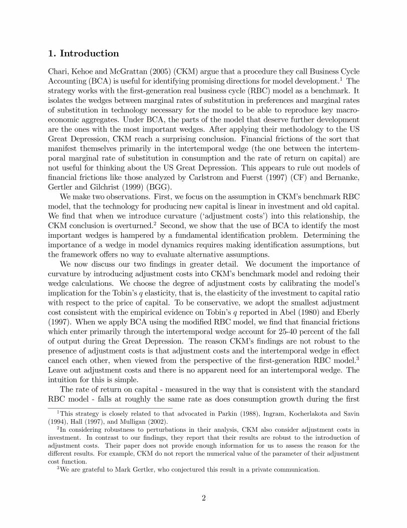
There are many C’s which satisfy this condition. In particular, write
C =
∙QW 00 q44
¸,
whereW is any orthonormal matrix. Each C in the above class is observationally equivalent,in that it implies the same likelihood value. However, each C implies a different et. To seethis, note that for any sequence of fitted disturbances, ut, one can recover a time series of etusing
et = C−1ut =
∙W 0Q−1 00 q−144
¸. (4.3)
To see how many et’s there are, for given V and sequence ut, let
a (θ1) =
⎡⎣ 1 0 00 cos (θ1) − sin (θ1)0 sin (θ1) cos (θ1)
⎤⎦ ,b (θ2) =
⎡⎣ cos (θ2) 0 sin (θ2)0 1 0
− sin (θ2) 0 cos (θ2)
⎤⎦ ,c (θ3) =
⎡⎣ cos (θ3) − sin (θ3) 0sin (θ3) cos (θ3) 00 0 1
⎤⎦W (θ) = a (θ1) b (θ2) c (θ3) ,
where θ = (θ1, θ2, θ3) and
θ ∈ D ≡ {θ : θi ∈ [0, 2π] , i = 1, 2, 3} .
Note that since a, b, and c are orthonormal, it follows that W (θ) is too, for each θ ∈ D. Fora fixed set of observed ut, t = 1, ..., T, there is a different sequence, et, t = 1, ..., T, associatedwith each θ ∈ D. The likelihood of the data is invariant to θ ∈ D.We adopt the normalization that the third element in et is the innovation in the shock
originating in the financial wedge. Each θ ∈ D adopts a different interpretation of the cross-shock correlations in the upper left block of V. For example, when θ = (0, 0, 0) , then et = εt.In this case, the third element of ut is entirely due to the innovation in the shock in thefinancial wedge, and all the correlation between the innovations in the wedges is attributedto causation going from the shock in the financial wedge to the other wedges.We will show that, because the data suggest that the off-diagonal terms in the upper
3 × 3 block of V are non-trivial, there are many different answers to question (i) in theintroduction: ‘what is the importance of the financial frictions shock?’ Each is equally likely,according to the likelihood function of the data.
5. Computing the Importance of the Intertemporal Wedge
In this section, we describe three procedures for computing the role of the intertemporalwedge in the dynamics of output, investment and employment in the 1930s. Each procedure
9
corresponds to a different way to isolate what would have happened if only the intertemporalwedge had been operative and none other. The first procedure (the ‘rotation decomposition’)is designed to illustrate our observations about identification in the previous section. Thesecond two procedures (the ‘impulse decomposition’ and the ‘expectation decomposition’)are alternative representations of the approach taken in CKM. Since the latter two produceroughly the same results, we only report results based on the impulse decomposition in thenext section.Our rotation procedure is as follows. We compute ut, t = 1929, ..., 1939, using (4.1).
Then, we fixW (θ) for some θ ∈ D and compute the implied sequence, et, for t = 1929, ..., 1939using (4.3). Then, to identify the importance of the shocks originating in the financial wedge,we set to zero all elements in et but the third one. After that, we compute the implied se-quence of disturbances, uWt , t = 1929, ..., 1939 using (4.2). Here, the superscript W appearsin order to highlight dependence on the orthonormal matrix,W. For input into our state space- observer system, (3.3)-(3.2), we require εt. We compute a sequence, εwt , t = 1929,...,1939using εWt = Q−1uWt . Thus, the mapping from the disturbances, ut, and θ ∈ D, to εWt is givenby:
εWt =
∙Q−1 00 q−144
¸ ∙QW (θ) 00 q44
¸⎡⎢⎢⎣0 0 0 00 0 0 00 0 1 00 0 0 0
⎤⎥⎥⎦∙ W (θ)0 Q−1 00 q−144
¸ut,
for t = 1929, ..., 1939. For each sequence, εWt , t = 1929, ..., 1939, we simulate (3.3)-(3.2) toobtain a time series on what investment, output and employment would have been had onlythe shocks originating in the intertemporal wedge (i.e., the third element of et) been active.We then compute the sum of squares of the discrepancy between the simulated investment,output and employment data, and choose θ ∈ D to minimize that discrepancy.13
The two versions of the CKM procedure are different ways to simulate the system inresponse to the realized intertemporal wedge, holding the other wedges fixed at their 1929values. We interpret this as reflecting the following two identification assumptions. The firstis that the whole of the movement in the intertemporal wedge reflects shocks originating inthe financial friction sector and the second is the notion that financial friction shocks do notinduce movements in the other wedges.For the impulse decomposition, we find the sequence, εt, t = 1929, ..., 1930 which has
the property that when this is input into (2.5), the third element of the simulated st, t =1929, ..., 1930, is set to its estimated values and the other elements of st are fixed at their 1929value. For the expectation decomposition, we adopt a different time series representationfor st. We suppose that only the third element of st is stochastic, while the other wedgesare simply constants at their 1929 values. The stochastic process that we adopt for theintertemporal wedge is the actual one obtained during the estimation. It is (2.5) itself,where the elements of st other than the third are simply treated as information variables.
13Our strategy of selecting a rotation based on the implied dynamic properties of a model resemblesidentification using sign restrictions, applied in, for example, Uhlig (2002).
10
6. Results
The results are presented in Figures 1-3 and Tables 1-3. The results in each of these figuresis based on the log-linear approximation to model solutions. The information in the tablesindicates that our results are robust to working with a second-order approximation.Consider Figure 1 first, which is based on the absence of investment adjustment costs,
a = 0. The first column reproduces the CKM results when a = 0. In the first, second andthird rows of graphs, the solid lines indicate the actual output, investment and hours workeddata, after removal of a log-linear trend. The lines with a ‘+’ indicate the movements ineach variable that is attributed to the intertemporal wedge. Note that the movement inoutput due to the intertemporal wedge, identified as CKM do, is trivial. The movement ininvestment and hours worked due to the intertemporal wedge are slightly greater, but stillnot very substantial. This corresponds to results reported in CKM.14
The second column of Figure 1 displays results based on our rotation decomposition. Theresults there show that it is possible to identify a rotation such that 100% of the movement inoutput, investment and hours throughout the 1930s is due to the intertemporal wedge. Thisillustrates our observations about identification. In particular, there is correlation amongthe wedges and without further structure, one is free to interpret this as causation passingfrom shocks originating in the intertemporal wedge, and inducing movements in the otherwedges. However, it is not clear that this finding poses a problem for the CKM conclusion.It is perhaps fair to interpret the results in the first and second columns of Figure 1 asindicating that if there are financial frictions, they manifest themselves primarily in non-intertemporal wedges. CKM emphasize that financial frictions of this kind are consistentwith the conclusions of their analysis. Of course, in practice the analyst would be leftguessing about whether this is a fair conclusion.Figure 2 repeats the calculations in Figure 1, with adjustment costs. Note that the results
are now very different. The results in the first column indicate that by the CKM metric, thedrop in output due to the intertemporal wedge is about 12 percent, or about 1/3 of the totalfall in output. Under the CKM identification, this suggests the intertemporal wedge is veryimportant. The wedge is even more important when we consider the fall in hours workedand investment.Column 2 provides illustrates the identification problem. The drop in output, investment
and hours worked in the first column of Figure 2 overstate the importance of the intertem-poral wedge to the extent that the movement in the intertemporal wedge reflects inducedeffects from shocks originating in other wedges. At the other extreme, the results in the firstcolumn of Figure 2 understates the importance of shocks emanating from the intertemporalwedge to the extent that those shocks also induce movements in the other wedges. To seehow important this second possibility can be, consider the second column of Figure 2. Therewe report the results based on a rotation in which shocks originating in the intertemporalwedge account for 100 percent of the movement in output, investment and hours workedthroughout the 1930s. The fact is that we cannot, using this framework, tell whether theintertemporal wedge accounts for 100 percent of the fall in output, 50 percent, or zero. A
14Actually, CKM report a slight rise in output, when the results are based on a non-linear solution of themodel. When we solve the model by a second order perturbation method, we find the same result. This willbe evident in the discussion of Table 1, below.
11
rotation can be found to yield either conclusion, and given the lack of structure in BCA, itis not possible to make a meaningful choice between them.To gain intuition into why it is that with a > 0 the importance of the intertemporal
wedge increases, consider Figure 3. The bottom row applies to the case, a = 0. The leftcolumn shows our estimate of the anticipated rate of return on capital, Et
¡1 +Rk
t+1
¢, for
the decade of the 1930s.15 Note how this quantity falls during this period. Note too, fromthe right column, that there is very little movement in the intertemporal wedge, τkt . Nowconsider the first row of graphs. With a > 0, Et
¡1 +Rk
t+1
¢actually rises as the economy
falls into Depression. Note that now there is a sharp rise in the intertemporal wedge. Thesefindings support the intuition described in the introduction.Tables 1-3 summarize our findings in tabular form. In addition, they provide evidence on
the robustness of our results to using a second-order approximation to our model solution.Each entry in these tables is:
1− data(wedge)1− data × 100.
Here, ‘data(wedge)’ denotes an estimate of what the (linearly detrended) data would havebeen if only the intertemporal wedge had been operative, normalized to unity in 1929. Also,‘data’ denotes the actual data, normalized by its 1929 value.Consider Table 1, which pertains to GNP only. The first two columns pertain to the
no adjustment cost case, in which case Tobin’s q is infinite. The results that pertain to thelinear approximation are transformations on the numbers displayed in Figure 1. Note how thepercent of the decline in output accounted for by the intertemporal wedge is relatively small.When we approximate the model solution with a second order approximation, the fall is evenless. Indeed, with the CKM identifying assumptions we conclude that the intertemporalwedge alone acted to raise output. Our findings confirm the results in CKM, who show thatwhen a nonlinear approximation is used to solve the model, the drop in output due to thewedge is smaller and actually becomes a rise.Note the very sharp contrast in the results when we move to the last two columns in
Table 1. When adjustment costs are incorporated into the analysis, and we adopt the CKMidentifying assumptions, we find that the intertemporal wedge accounts for 25-40 percentof the drop in output. Both linear and nonlinear approximations generate similar results.The results in Table 2 show that with adjustment costs, under the CKM identificationassumptions the intertemporal wedge accounts for a huge portion of the decline in investment.According to Table 3, the fraction of the drop in hours worked due to the intertemporal wedgeis roughly similar to what we found for output.In sum, we find that with adjustment costs and with the CKM identification assumptions,
the intertemporal wedge has a substantial impact on the major macroeconomic variables dur-ing the Great Depression. However, these results are dependent on the CKM identificationassumptions. Other identification assumptions are observationally equivalent. There aresome that support the view that the intertemporal wedge had virtually nothing to do withthe Great Depression. Others support the view that the only wedge that mattered was theintertemporal wedge.
15We estimated this variable by including it in the state evolution of our Kalman filter system, and thenusing the two-sided Kalman smoother.
12
7. Conclusion
Chari, Kehoe and McGrattan (2005) advocate the use of ‘wedges’ to identify directions forimprovement in equilibrium models. As a demonstration of the power of the approach theyargue that it can be used to rule out a prominent class of explanations for the Great Depres-sion. In particular, they conclude that models of financial frictions that create wedges in theintertemporal Euler equation are not promising avenues for understanding the dynamics ofthe Great Depression.We show that the conclusions are not robust to a small change in CKM’s model environ-
ment. In particular, when a modest amount of investment adjustment costs are introduced,we find that the CKM findings about financial frictions are reversed. We also show thatbusiness cycle accounting suffers from a significant identification problem: determining theimportance of a wedge requires identifying assumptions, and there is no way to choosebetween the alternative possibilities. The problem is similar to the well known problemof identification in a vector autoregression (VAR). Fundamental economic shocks are notidentified in VARs. Additional restrictions must be incorporated from economic theory ifquestions about the importance of particular economic shocks, such as financial frictionsshocks, are to be answered.Fortunately, there are other methods to identify promising avenues for model develop-
ment. Computational methods, software and econometric methods have now reached a stagewhere it is straightforward to specify and evaluate alternative model specifications quicklyand efficiently. There is no reason to guess what these explorations are likely to produceusing a method like business cycle accounting.16
16This strategy for determining the importance of financial frictions is pursued by Christiano, Motto andRostagno (2004, 2005). They use likelihood methods to investigate the role of financial frictions as sourcesof shocks and propagation in the US Great Depression and in recent business cycles in the Euro Area andthe US.
8. Appendix A: The Carlstrom-Fuerst Financial Friction Wedge
This section considers a version of the CF model, modified to include the adjustment costsin capital considered in CKM. We identify the version of the RBC model with wedges whoseequilibrium coincides with that of the CF model with adjustment costs. We state the resultas a proposition. For the RBC wedge economy to have literally the same equilibrium asthe CF economy with adjustment costs requires several wedges and other adjustments. Wethen describe the parameter settings required in the original CF model to ensure that theadjustments primarily take the form of a wedge in the intertemporal Euler equation, andnowhere else. In this respect we follow the approach taken in CKM. To simplify the notation,we set the population growth rate to zero throughout the discussion in the appendix.
8.1. RBC Model With Adjustment Costs
To establish a baseline, we describe the version of the RBC model with adjustment costs.Preferences are:
E0
∞Xt=0
βtu (ct, lt) .
The resource constraint and the capital accumulation technology are, respectively,
ct + xt ≤ kαt (Ztlt)1−α (8.1)
and
kt+1 = (1− δ) kt + xt − Φ
µxtkt
¶kt. (8.2)
The first order necessary conditions for optimization are:
−ul,tuc,t
= (1− α)
µktlt
¶α
Z1−αt (8.3)
1 = βEtuc,t+1uc,t
¡1 +Rk
t+1
¢, (8.4)
where the gross rate of return on capital is:
1 +Rkt+1 =
α³
kt+1Zt+1lt+1
´α−1+ Pk,t+1
Pk0t.
where Pk,t and Pk0,t are given in (2.9) and (2.10).In the following two subsections, we argue that the CF financial frictions act like a tax
on the gross return on capital, 1 +Rkt+1, in (8.4). In particular, 1 +Rk
t+1 is replaced by¡1 +Rk
t+1
¢ ¡1− τkt
¢.
This statement is actually only true as an approximation. Below we state, as a proposition,what the exact RBC model with wedges is, which corresponds to the CF model. We thenexplain the sense in which the wedge equilibrium just described is an approximation.
15
8.2. The CF Model With Adjustment Costs
Here, we develop the version of the CF model in which there are adjustment costs in theproduction of new capital. The economy is composed of firms, an η mass of entrepreneurs anda mass, 1−η, of households. The sequence of events through the period proceeds as follows.First, the period t shocks are observed. Then, households and entrepreneurs supply labor andcapital to competitive factor markets. Because firm production functions are homogeneous,all output is distributed in the form of factor income. Households and entrepreneurs then selltheir used capital on a capital market. The total net worth of households and entrepreneurs atthis point consists of their earnings of factor incomes, plus the proceeds of the sale of capital.Households divide this net worth into a part allocated to current consumption, and a partthat is deposited in the bank. Entrepreneurs apply their entire net worth to a technologyfor producing new capital. They produce an amount of capital that requires more resourcesthan they can afford with only their own net worth. They borrow the rest from banks.At this point the entrepreneur experiences an idiosyncratic shock which is observed to him,while the bank can only see it by paying a monitoring cost. This creates a conflict betweenthe entrepreneur and the bank which is mitigated by the bank extending the entrepreneur astandard debt contract. After capital production occurs, entrepreneurs sell the new capital,and pay off their bank loan. Households receive a return on their deposits at the bank, anduse the proceeds to purchase new capital. Entrepreneurs use their income after paying offthe banks to buy consumption goods and new capital. All the newly produced capital ispurchased by households and entrepreneurs, and all the economy’s consumption goods areconsumed. The next period, everything starts all over.We now provide a formal description of the economy. The household problem is
max{cc,t,kct+1}∞t=0
∞Xt=0
βtu (ct, lt) ,
subject to:ct + qtkc,t+1 ≤ wc
t lt + [rt + Pk,t] kc,t (8.5)
where ct and kc,t denote household consumption and the household stock of capital, re-spectively. In addition, and lt denotes household employment, wc
t denotes the household’scompetitive wage rate, Pk,t denotes the price of used capital and qt denotes the price of capi-tal available for production in the next period (the reason for not denoting this price by Pk0,t
will be clear momentarily). After receiving their period t income, households allocate theirnet worth (the right side of (8.5)) to ct and the rest, wc
t lt+[rt + Pk,t] kc,t−ct, is deposited in abank. These deposits earn a rate of return of zero. This is because markets are competitiveand the opportunity cost to the household of the output they lend to the bank is zero. Laterin the period, when the deposit matures, the households use the principal to purchase kc,t+1units of capital. The first order conditions of the household are (8.5) with the equality strictand:
1 = Etβuc,t+1uc,t
∙rt+1 + Pk,t+1
qt
¸(8.6)
−ul,tuc,t
= wet , (8.7)
16
where uc,t and −ul,t denote the time t marginal utilities of consumption and leisure, respec-tively.The η entrepreneurs’ present discounted value of utility is:
E0
∞Xt=0
(βγ)t cet.
After the period t shocks are realized, the net worth of entrepreneurs, at, is:
at = wet + [rt + Pk,t] ket,
where wet is the wage rate earned by the entrepreneur, who inelastically supplies his one unit
of labor. The entrepreneur uses the at consumption goods, together with a loan from thebank to purchase the inputs into the production of capital goods. Entrepreneurs have accessto the technology for producing capital, (2.6) and (2.7). The technology proceeds in twostages. In the first stage, the entrepreneur produces an intermediate input, it. In the secondstage, that input results in ωit units of capital, which has a price, in consumption goods, qt.The random variable, ω, is independently distributed across entrepreneurs, has mean unity,and cumulative density function,
Ψ (z) ≡ prob [ω ≤ z] .
The entrepreneur who wishes to produce it units of the capital input faces the followingcost function:
C (it;Pk,t) = minϕk,t,ϕx,t
Pk,tϕk,t + ϕx,t + λt
∙it − (1− δ)ϕk,t − ϕx,t + Φ
µϕx,t
ϕk,t
¶ϕk,t
¸,
where the constraint is that the object in square brackets is no less than zero. In addition,ϕk,t and ϕx,t denote the quantity of old capital and investment goods, respectively, purchasedby the entrepreneur. The first order conditions for ϕk,t and ϕx,t are:
Pk,t = λt
∙1− δ − Φ
µϕx,t
ϕk,t
¶+ Φ0
µϕx,t
ϕk,t
¶ϕx,t
ϕk,t
¸(8.8)
1 = λt
∙1− Φ0
µϕx,t
ϕk,t
¶¸, (8.9)
respectively. The reason for denoting the time t price of old capital by Pk,t is now apparent.Substituting out for λ in (8.8) from (8.9), we see that the formula for Pk,t here coincideswith with the one implied by (2.9)-(2.10). The reason for not denoting the price of newcapital by Pk0,t is also apparent. Comparing (8.9) with (2.9)-(2.10) we see that the formulafor λt coincides with the formula for Pk0,t implied by (2.9)-(2.10). However, the equilibriumvalue of qt will not coincide with λt here. This is because λt does not capture all the costs ofproducing new capital. It measures the marginal costs implied by the production technology.However, it is missing the marginal cost that arises from the conflict between entrepreneursand banks, which has the consequence that the production of capital necessarily involvessome monitoring, and therefore also involves some destruction of capital.
17
Solving (8.9) for xt/kt in terms of λt, and using the result to substitute out for ϕx,t/ϕk,t
in (8.8):
Pk,t = λt
⎡⎣(1− δ)− a
2
Ã1λt− 1a
!2+ a
Ã1λt− 1a
!Ã1λt− 1a
+ b
!⎤⎦Solving this for λt, provides the marginal cost function for producing it :
λt = λ (Pk,t) . (8.10)
Because all entrepreneurs face the same Pk,t, they will all choose the same ratio, ϕx,t/ϕk,t,regardless of the scale of production, it. Moreover, that ratio must be equal to the ratio ofaggregate investment to the aggregate stock of capital.The constant returns to scale feature of the production function implies that the total
cost of producing it is:
C (it;Pk,t) =
½λ (Pk,t) it a > 0
it a = 0
Consider an entrepreneur who has at units of goods and wishes to produce it ≥ at, so that theentrepreneur must borrow λ (Pk,t) it− at from the bank. Following CF, we suppose that theentrepreneur receives a standard debt contract. This specifies a loan amount and an interestrate, Ra
t , in consumption units. If the revenues of the entrepreneur turn out to be too low forhim to repay the loan, then the entrepreneur is ‘bankrupt’ and he simply provides everythinghe has to the bank. In this case, the bank pays a monitoring cost which is proportional tothe scale of the entprepeneur’s project, µiat . We now work out the equilibrium value of theparameters of the standard debt contract.The value of ω such that entrepreneurs with smaller values of ω are bankrupt, is ωa
t ,where
[λ (Pk,t) it − at]Rat = ωa
t itqt.
Using this we find that the average, across all entrepreneurs with asset level at, of revenuesis:
itqt
Z ∞
0
ωdF (ω)−Z ∞
ωat
Rat (λ (Pk,t) i
at − at) dF (ω)− itqt
Z ωat
0
ωdF (ω)
= itqtf (ωat ) ,
where
f (ωat ) =
Z ∞
ωat
ωdΦ (ω)− ωat (1− Φ (ωa
t )) .
The average receipts to banks, net of monitoring costs, across loans to all entprepreneurswith assets at is:
qtiat
∙Z ωat
0
ωdΦ (ω)− µΦ (ωat )
¸+ [λ (Pk,t) it − at]R
at [1− Φ (ωa
t )]
= qtiat g (ω
at ) ,
18
where
g (ωat ) =
Z ωat
0
ωdΦ (ω)− µΦ (ωat ) + ωa
t [1− Φ (ωat )] .
The contract with entrepreneurs with asset levels, at, that is assumed to occur in equi-librium is the one that maximizes the expected state of the entrepreneur at the end of thecontract, subject to the requirement that the bank be able to pay the household a grossrate of interest of unity. The interval during which the entrepreneur produces capital is onein which there is no alternative use for the output good. So, the condition that must besatisfied for the bank to participate in the loan contract is:
qtitg (ωat ) ≥ λ (Pk,t) it − at.
The contract solves the following Lagrangian problem:
maxωat ,it
itqtf (ωat ) + µ [qtitg (ω
at )− λ (Pk,t) it + at] .
The first order conditions for ωat and it are, after solving out for µ and rearranging:
qtf (ωat ) =
f 0 (ωat )
g0 (ωat )[qtg (ω
at )− λ (Pk,t)] (8.11)
it =at
λ (Pk,t)− qtg (ωat )
(8.12)
From (8.11), we see that ωat = ωt for all at, so that Ra
t = Rt for all at. It then follows from(8.12) that the loan amount is proportional to at. As in the no adjustment case in CF, thesetwo properties imply that in studying aggregates, we can ignore the distribution of assetsacross entrepreneurs.The expected net revenues of the entrepreneurs, expressed in terms of at, are, after making
use of (8.12):
itqtf (ωt) =qtf (ωt)
λ (Pk,t)− qtg (ωt)at. (8.13)
At the end of the period, after the debt contract with the bank is paid off, the entrepreneurswho do not go bankrupt in the process of producing capital have income that can be usedto buy consumption goods and new capital goods:
cet + qtket+1 ≤½
itqtω −Rt (λ (Pk,t) it − at) ω ≥ ωt
0 ω < ωt. (8.14)
An entrepreneur who is bankrupted in period t must set cet = 0 and ket+1 = 0. In periodt + 1, these entrepreneurs start with net worth at+1 = we
t+1. Entrepreneurs who are notbankrupted in period t can purchase positive amounts of cet and ke,t+1 (except in the non-generic case, ω = ωt). For these entrepreneurs, the marginal cost of purchasing ke,t+1 is qtunits of consumption. The time t expected marginal payoff from ke,t+1 at the beginning ofperiod t + 1 is Et [rt+1 + Pk,t+1] . In each aggregate state in period t + 1, the entrepreneurexpands his net worth by the value of [rt+1 + Pk,t+1] in that state. This extra net worthcan be leveraged into additional bank loans, which in turn permit an expansion in the
19
entrepreneur’s payoff by investing in the capital production technology. The expected valueof this additional payoff (relative to date t+1 idiosyncratic uncertainty) corresponds to thecoefficient on at in (8.13). So, the expected rate of return available to entrepreneurs who arenot bankrupt in period t is:
Et
∙rt+1 + Pk,t+1
qt× ζt+1
¸, (8.15)
which they equate to 1/(βγ). Here,
ζt+1 = max
∙qt+1f (ωt+1)
λ (Pk,t+1)− qt+1g (ωt+1), 1
¸.
The expression to the left of ‘×’ in (8.15) is the rate of return enjoyed by ordinary households.The reason that ζt+1 cannot be less than unity is that and entprepeneur can always obtainunity, simply by consuming his net worth in the following period and not producing anycapital. Averaging over all budget constraints in (8.14):
cet + qtket+1 =qtf (ωt)
λ (Pk,t)− qtg (ωt)at.
Here, cet and ke,t+1 refer to averages across all entrepreneurs.Output is produced by goods-producers using a linear homogeneous technology,
where kt is the sum of the capital owned by households and the average capital held byentrepreneurs:
kt = (1− η) kct + ηke,t.
The argument, η, in y is understood to apply to the second occurrence of η. The argumentsin the production function reflect our assumption that the entrepreneur supplies one unit oflabor, and households supply lt units of labor. Profit maximization implies:
yk,t = rt, yl,t = wct , y3,t = we
t . (8.17)
We now collect the equilibrium conditions for the economy. The production of new capitalgoods by the average entrepreneurs is:
it
Z ∞
0
ωdF (ω)− µit
Z ωt
0
dF (ω)
= it [1− µF (ωt)] .
Since there are η entprepreneurs, the total new capital produced is kt+1 = ηit [1− µF (ωt)] ,so that
The budget constraint of the entrepreneur is (after multiplying by η) :
cet + qtket+1 = λ (Pk,t)kt+1
η [1− µF (ωt)]qtf (ωt) (8.22)
The efficiency conditions associated with the contract are:
qtf (ωt) =f 0 (ωt)
g0 (ωt)[qtg (ωt)− λ (Pk,t)] (8.23)
kt+1η [1− µF (ωt)]
=at
λ (Pk,t)− qtg (ωt)(8.24)
at = y3,t + yk,tket + Pk,tket (8.25)
The intertemporal efficiency condition for the entrepreneur is (assuming the condition, ζt+1 ≥1, is not binding):
Et
∙Fk,t+1 + Pk,t+1
qt× qt+1f (ωt+1)
λ (Pk,t+1)− qt+1g (ωt+1)
¸=1
γβ(8.26)
Taking the ratio of (8.8) to (8.9), we obtain:
Pk,t =1− δ − Φ
³xtkt
´+ Φ0
³xtkt
´xtkt
1− Φ0³xtkt
´ (8.27)
The 10 variables to be determined with the 10 equations, (8.18)-(8.27) are: ct, ce,t, xt, kt,ke,t, lt, Pk,t, qt, ωt, at.It is convenient to define a sequence of markets equilibrium formally. Let st denote a
history of realizations of shocks. Then,
Definition 8.1. An equilibrium of the CF economy with adjustment costs is a sequence ofprices, {Pk (s
t) , q (st) , we (st) , wc (st) , r (st)} , quantities, {c (st) , ce (st) , x (st) , k (st) , ke (st) , l (st) , a (st)} ,and {ω (st)} such that:(i) Households optimize (see (8.20), (8.21))(ii) Entrepreneurs optimize (see (8.22), (8.25), (8.26), (8.27))(iii) Firms optimize (see (8.17))(iv) Conditions related to the standard debt contract are satisfied (see (8.23), (8.24))(v) The resource constraint and capital accumulations equations are satisfied (see (8.18),
(8.19))
21
8.3. The CF Model as an RBC Model with Wedges
We now construct a set of wedges for the RBC economy, such that the equilibrium for thateconomy coincides with the equilibrium for the CF economy. We begin by constructing thefollowing state-contingent sequences:
ψ¡st¢= 1− µF
¡eω ¡st¢¢ , (8.28)
τx¡st¢=
ψ (st) q (st)
λ³Pk,t (st)
´ − 1,θ¡st¢=
Pk (st) τx (s
t)
r (st),
G¡st¢= η
¡ce¡st¢− c
¡st¢¢
,
T¡st¢= G
¡st¢− τx
¡st¢x¡st¢− θ
¡st¢r¡st¢k¡st−1
¢,
D¡st¢= we
¡st¢η,
where q, ce, c, we, r, k, x, eω and Pk correspond to the objects without ‘ · ’ in a CF equilibrium.Also, λ is the function defined in (8.10). In this subsection, we treat D, ψ, θ, τx, G and Tas given exogenous stochastic processes. Here, D, G, and T represent exogenous sequencesof profits, government spending and lump sum taxes. Also, θ and τx are tax rates oncapital rental income and investment good purchases. Finally, ψ is a technology shock inthe production of physical capital.Consider the following budget constraint for the household:
c¡st¢+¡1 + τx
¡st¢¢
x¡st¢
(8.29)
≤¡1− θ
¡st¢¢
r¡st¢k¡st−1
¢+ w
¡st¢l¡st¢− T
¡st¢+D
¡st¢.
Here, r is the rental rate on capital, w is the wage rate, and l measures the work effort of thehousehold. Each of these variables is a function of st and is determined in an RBC wedgeeconomy. At time 0 the household takes prices, taxes and k (s−1) as given and chooses c, kand l to maximize utility:
∞Xt=0
Xst
βtπ¡st¢u¡c¡st¢, l¡st¢¢
subject to the budget constraint and non-negativity constraints. Here, π (st) is the proba-bility of history, st.Households operate the following backyard technology to produce new capital:
k¡st¢=
∙(1− δ) k
¡st¢+ x
¡st¢− Φ
µx (st)
k (st−1)
¶k¡st−1
¢¸ψ¡st¢. (8.30)
22
The first order necessary conditions for household optimization are:
ul¡st¢+ uc
¡st¢w¡st¢= 0, (8.31)
1 + τx (st)
ψ (st)Pk0¡st¢
(8.32)
=Xst+1|st
βπ¡st+1|st
¢ uc (st+1)uc (st)
£r¡st+1
¢ ¡1− θ
¡st+1
¢¢+¡1 + τx
¡st+1
¢¢Pk
¡st+1
¢¤,
where
Pk
¡st¢≡1− δ − Φ
µx(st)k(st)
¶+ Φ0
µx(st)k(st)
¶x(st)k(st)
1− Φ0³
x(st)k(st−1)
´ . (8.33)
Equation (8.31) is the first order condition associated with the optimal choice of l (st) .Equation (8.32) combines the first order order conditions associated with the optimal choiceof x (st) and k (st) . Also,
Pk0¡st¢≡ 1
1− Φ0³
x(st)k(st−1)
´ , (8.34)
is the pre-tax marginal cost of producing new capital, in units of the consumption good. Inaddition, π (st+1|st) ≡ π (st+1) /π (st) is the conditional probability of history st+1 given st.The technology for firms is taken from (8.16):
y (k, l, η, Z) = kα ((1− η)Zl)1−α−ζ ηζ ,
where, as before, the third argument in y refers only to the second occurrence of η. There arethree inputs: physical capital, household labor and another factor whose aggregate supplyis fixed at η. Profit maximization leads to:
r¡st¢= yk
¡st¢, w
¡st¢= yl
¡st¢, we
¡st¢= yη
¡st¢. (8.35)
The household is assumed to own the representative firm, and it receives the earnings ofη in the form of lump-sum profits, D (st) . We do allow allow trade in claims on firms, arestriction that is non-binding on allocations because the households are identical.We now state the equilibrium for the RBC wedge economy:
Definition 8.2. AnRBCwedge equilibrium is a set of quantities, {c (st) , l (st) , k (st) , x (st)} ,and prices {Pk (s
t) , Pk0 (st) , r (st) , w (st)} , and a set of taxes, profits and government spend-
ing, {G (st) , τx (st) , θ (st) , T (st)} , technology shocks, {Z (st) , ψ (st)} , such that(i) The quantities solve the household problem given the prices, taxes, profits, government
spending and the shock to the backyard investment technology(ii) Firm optimization is satisfied(iii) Relations (8.28) is satisfied, for given state-contingent sequences, q, ce, c, we, r, k,
x, eω and Pk.
23
The variables to be determined in an RBC wedge equilibrium are c, l, k, x, Pk, Pk0 , r andw. The 8 equations that can be used to determine these are (8.29)-(8.35). It is easily verifiedthat c, l, k, x, Pk, r and w coincide with the corresponding objects in a CF equilibrium. Inaddition, Pk0 coincides with λ (Pk) in a CF equilibrium. To see this, one verifies that theequilibrium condition in the RBC wedge economy coincides with the equilibrium conditionsin the CF economy. First, (8.30) coincides with (8.18). After using (8.35), we see that(8.31) coincides with (8.21). Consider the household budget equation evaluated at equality.Substituting out for lump sum transfers:
c¡st¢+¡1 + τx
¡st¢¢
x¡st¢
=¡1− θ
¡st¢¢
r¡st¢k¡st−1
¢+ w
¡st¢l¡st¢
τx¡st¢x¡st¢+ θ
¡st¢r¡st¢k¡st−1
¢+ we
¡st¢η +G
¡st¢,
or,
(1− η) c¡st¢+ x
¡st¢+ ηce
¡st¢
(8.36)
= r¡st¢k¡st−1
¢+ w
¡st¢l¡st¢+ we
¡st¢η
= y¡k¡st−1
¢, l¡st¢, η, Z
¡st¢¢
,
by linear homogeneity. Here, Z (st) = Z (st) , where st is the realization of period t uncertainty.Equation (8.36) coincides with (8.19). Substitute out for θ and τx from (8.28) into (8.32),and rearranging, we obtain:
1 = Etuc (s
t+1)
uc (st)
"r (st+1) + Pk (s
t+1)1+τx(st)ψ(st)
Pk0 (st)
#.
Note that by definition of 1 + τx (st) in (8.28),
1 + τx (st)
ψ (st)Pk0¡st¢=
Pk0 (st) q (st)
λ (Pk,t (st)).
Combining (8.10) and (8.9), we find that λ (Pk,t (st)) = Pk0 (s
t) , so that the household’sintertemporal Euler equation reduces to (8.20), or (after making use of (8.35)):
Etuc (s
t+1)
uc (st)
∙yk (s
t+1) + Pk (st+1)
Pk0 (st)
¡1− τk
¡st¢¢¸
= 1, (8.37)
where
1− τk¡st¢=
ψ (st)
1 + τx (st).
We conclude that conditions (8.18)-(8.21) in the CF economy are satisfied. The remainingequilibrium conditions are satisfied, given (8.28). We state this result as a proposition:
Proposition 8.3. Consider a CF equilibrium, and a set of taxes, technology shocks andtransfers computed in (8.28). The objects, {c (st) , l (st) , k (st) , x (st)} , {Pk (s
t) , r (st) , w (st)}and Pk0 (s
t) = λ (Pk (st)) in the CF equilibrium correspond to an RBC wedge equilibrium.
For η and ζ close to zero and ψ close to unity, the RBC wedge equilibrium converges tothe equilibrium conditions of the RBC model with adjustment costs in section 8.1 with awedge, 1− τk, in the intertemporal Euler equation, (8.4).
24
9. Appendix B: The Bernanke-Gertler-Gilchrist Financial FrictionWedge
In this section we briefly review the BGG model and derive the RBC wedge model to whichit corresponds. In the model there are households, capital producers, entrepreneurs andbanks. At the beginning of the period, households supply labor to factor markets, andentrepreneurs supply capital. Output is then produced and an equal amount of incomeis distributed among households and entrepreneurs. Households then make a deposit withbanks, who lend the funds on to entrepreneurs. Entrepreneurs have a special expertise in theownership and management of capital. They have their own net worth with which to acquirecapital. However, it is profitable for them to leverage this net worth into loans from banks,and acquiring more capital than they can afford with their own resources. The source offriction is a particular conflict between the entrepreneur and the bank. In the managementof capital, idiosyncratic things happen, which either make the management process moreprofitable than expected, or less so. The problem is that the things that happen in thisprocess are observed only by the entrepreneur. The bank can observe what happens insidethe management of capital, but only at a cost. As a result, the entrepreneur has an incentiveto underreport the results to the bank, and thereby attempt to keep a greater share of theproceeds for himself. To mitigate this conflict, it is assumed that entrepreneurs receive astandard debt contract from the bank.The capital that entrepreneurs purchase at the end of the period is sold to them by
capital producers. The latter use the old capital used within the period, as well as investmentgoods, to produce the new capital that is sold to the entrepreneurs. Capital producers haveno external financing need. They finance the purchase of used capital and investment goodsusing the revenues earned from the sale of new capital.The budget constraint of households is:
ct +Bt+1 ≤ (1 +Rt)Bt + wtlt + Tt,
where Rt denotes the interest earned on deposits with the bank, bt denotes the beginning-of-period t stock of those deposits, wt denotes the wage rate, lt denotes employment and Ttdenotes lump sum transfers. Subject to this budget constraint and a no-Ponzi condition,households seek to maximize utility:
E0
∞Xt=0
βtu (ct, lt) .
Households’ first order conditions, in addition to the transversality condition, are:
uc,t = βEtuc,t (1 +Rt+1)−ul,tuc,t
= wt.
Firms have the following production function:
yt = kαt (Ztlt)1−α = y (kt, lt, Zt) .
25
They rent capital and hire labor in perfectly competitive markets at rental rate, rt, and wagerate, wt, respectively. Optimization implies:
yk,t = rt, yl,t = wt.
Capital producers purchase investment goods, xt, and old capital, kt, to produce newcapital, kt+1, using the following linear homogeneous technology:
kt+1 = (1− δ) kt + xt − Φ
µxtkt
¶kt.
The competitive market prices of kt and kt+1 are Pk,t and Pk0,t, respectively. Capital produceroptimization leads to the following conditions:
Pk,t =1
1− Φ0³xtkt
´ ∙1− δ − Φ
µxtkt
¶+ Φ0
µxtkt
¶xtkt
¸
Pk0,t =1 + gn
1− Φ0³xtkt
´ .At the end of period t, entrepreneurs have net worth, Nt+1, and it is assumed that
Nt+1 < Pk0,tkt+1. As a result, in an equilibrium in which the entire stock of capital is to beowned and operate, entprepreneurs must borrow:
bt+1 = Pk0,tkt+1 −Nt+1. (9.1)
As soon as an individual entrepreneur purchases kt+1, he experiences a shock, and kt+1becomes kt+1ω. Here, ω is a random variable that is iid across entrepreneurs and has meanunity. The realization of ω is unknown before the loan is made and it is known only to theentrepreneur after it is realized. The bank which extends the loan to the entrepreneur mustpay a monitoring cost in order to observe the realization of ω. The cumulative distributionfunction of ω is F, where
Pr ob [ω < x] = F (x) .
Entrepreneurs receive a standard debt contract from their bank, which specifies a loanamount, bt+1, and a gross rate of return, Zt+1, in the event that it is feasible for the en-trepreneur to repay. The lowest realization of ω for which it is feasible to repay is ωt+1,where
ωt+1
¡1 +Rk
t+1
¢Pk0,tkt+1 = Zt+1bt+1. (9.2)
For ω < ωt+1 the entrepreneur simply pays all its revenues to the bank:¡1 +Rk
t+1
¢ωPk0,tkt+1.
In this case, the bank monitors the entrepreneur. Following BGG, we assume that monitoringcosts are a fraction, µ, of the total earnings of the entrepreneur:
µ¡1 +Rk
t+1
¢ωPk0,tkt+1.
26
The bank’s source of funds is the deposits of households, and so for each amount thebank lends, it must pay a gross rate of return, 1 +Rt+1. Competition and non-negativity ofprofits implies that banks make zero profits in each date and state. The zero profit conditionis:
[1− F (ωt+1)]Zt+1bt+1 + (1− µ)
Z ωt+1
0
ωdF (ω)¡1 +Rk
t+1
¢Pk0,tkt+1 =
¡1 +Re
t+1
¢bt+1.
Substituting from (9.2) for Zt+1bt+1 and dividing by¡1 +Rk
t+1
¢Pk0,tkt+1 :
[1− F (ωt+1)] ωt+1 + (1− µ)
Z ωt+1
0
ωdF (ω) =
µ1 +Re
t+1
1 +Rkt+1
¶bt+1
Pk0,tkt+1.
We conclude that the gross return on capital can be expressed:
1 +Rt+1 =¡1− τkt+1
¢ ¡1 +Rk
t+1
¢,
where the ‘wedge’, 1− τkt+1, satisfies:
1− τkt+1 =Pk0,tkt+1 −Nt+1
Pk0,tkt+1
µ[1− F (ωt+1)] ωt+1 + (1− µ)
Z ωt+1
0
ωdF (ω)
¶.
The wedge, τkt , contains two additional endogenous variables, Nt+1 and ωt+1. These aredetermined in general equilibrium by the introduction of two additional equations: the con-dition associated with the fact that the standard debt contract maximizes the utility of theentrepreneur, as well as the law of motion for entrepreneurial net worth.The resource constraint for this economy is:
ct +Gt + xt = kαt (Ztlt)1−α ,
where Gt includes any consumption of entrepreneurs, as well as monitoring costs incurredby banks. As long as these latter can be ignored, then the BGG financial frictions is to, ineffect, introduce a tax on the rate of return on capital in, 1 + Rk
t+1, in (8.4). In particular,1 +Rk
t+1 is replaced by ¡1 +Rk
t+1
¢ ¡1− τkt+1
¢.
Note there is a slight difference with CF financial frictions in that the latter imply the taxrate is not a function of period t + 1 uncertainty, while the BGG frictions imply that ingeneral it is a function of this uncertainty.
27
References
[1] Abel, Andrew, 1980, “Empirical investment equations: An integrative framework,”Carnegie-Rochester Conference Series on Public Policy, vol. 12, pp. 39—91.
[2] Bernanke, Ben, Mark Gertler, and Simon Gilchrist, 1999, “The Financial Acceleratorin a Quantitative Business Cycle Framework,” Handbook of Macroeconomics, editedby John B. Taylor and Michael Woodford, pp. 1341-1393, Amsterdam, New York andOxford, Elsevier Science, North-Holland.
[3] Carlstrom, Charles, and Timothy Fuerst, 1997, “Agency Costs, Net Worth, and Busi-ness Fluctuations: A Computable General Equilibrium Analysis,” American EconomicReview, 87, 893-910.
[4] Chari, V.V., Patrick Kehoe and Ellen McGrattan, 2005, “Business Cycle Accounting,”Federal Reserve Bank of Minneapolis Staff Report 328, revised April.
[5] Christiano, Lawrence J., 2002, ‘Solving Dynamic Equilibrium Models by a Method ofUndetermined Coefficients,’ Computational Economics.
[6] Christiano, Lawrence J., Roberto Motto and Massimo Rostagno, 2004, ‘The US GreatDepression and the Friedman-Schwartz Hypothesis,’ Journal of Money, Credit andBanking.
[7] Christiano, Lawrence J., Roberto Motto and Massimo Rostagno, 2005, ‘Financial Fac-tors in Business Cycles,’ manuscript.
[8] Eberly, Janice C., 1997, ‘International Evidence on Investment and Fundamentals,’European Economic Review, vol. 41, no. 6, June, pp. 1055-78.
[9] Fernandez-Villaverde, Jesus, Juan F. Rubio-Ramirez and Thomas J. Sargent, 2005, ‘A,B, C ’s (and D)’s For Understanding VARs,’ manuscript, March 18.
[10] Hall, Robert, 1997, ‘Macroeconomic Fluctuations and the Allocation of Time,’ Journalof Labor Economics, 15 (part 2) , S223-S250.
[11] Hamilton, James B. (1994). Time Series Analysis. Princeton: Princeton UniversityPress.
[12] Hansen, Lars P., and Kenneth Singleton, 1982, “Generalized Instrumental VariablesEstimation of Nonlinear Rational Expectations Models,” Econometrica 50, 1269-1286.
[13] Hansen, Lars P., and Kenneth Singleton, 1983, “Stochastic Consumption, Risk Aversion,and Temporal Behavior of Asset Returns,” Journal of Political Economy, 91, 249-268.
[14] Ingram, Beth, Narayana Kocherlakota and N. Savin, 1994, “Explaining Business Cycles:A Multiple-Shock Approach,” Journal of Monetary Economics, 34, 415-428.
28
[15] Kim, Jinill, Sunghyum Kim, Ernst Schaumburg, and Christopher Sims, 2005, ‘Calculat-ing and Using Second Order Accurate Solutions of Discrete Time Dynamic EquilibriumModels,’ manuscript, February 3.
[16] Mulligan, Casey, 2002, ‘A Dual Method of Empirically Evaluating Dynamic CompetitiveModels with Market Distortions, Applied to the Great Depression and World War II,’National Bureau of Economic Research Working Paper 8775.
[17] Parkin, Michael, 1988, ‘A Method for Determining Whether Parameters in AggregativeModels are Structural,’ Carnegie-Rochester Conference Series on Public Policy, 29, 215-252.
[18] Primiceri, Giorgio, Ernst Schaumburg and Andrea Tambalotti, 2005, “IntertemporalDisturbances,” manuscript, Northwestern University.
[20] Wan, E.A. and R. van der Merwe, 2001, "Kalman Filtering and Neural Networks",chap. Chapter 7 : The Unscented Kalman Filter, (50 pages), Wiley Publishing, Eds. S.Haykin.
29
1930 1932 1934 1936 1938
0.7
0.8
0.9
1Impulse Decomposition: GDP
1930 1932 1934 1936 19380.65
0.7
0.75
0.8
0.85
0.9
0.95
Rotation Decomposition: GDP
1930 1932 1934 1936 1938
0.4
0.6
0.8
1
Impulse Decomposition: INV
1930 1932 1934 1936 19380.3
0.4
0.5
0.6
0.7
0.8
0.9
Rotation Decomposition:INV
1930 1932 1934 1936 1938
0.75
0.8
0.85
0.9
0.95
1
Impulse Decomposition: HOURS
1930 1932 1934 1936 1938
0.75
0.8
0.85
0.9
0.95
1Rotation Decomposition: HOURS
1930 1932 1934 1936 19380.4
0.5
0.6
0.7
0.8
0.9
1
Efficiency Wedge
1930 1932 1934 1936 19380.4
0.5
0.6
0.7
0.8
0.9
1
Labor Wedge
1930 1932 1934 1936 19380.4
0.5
0.6
0.7
0.8
0.9
1
Intertemporal Wedge
Figure 1: Wedges With No Adjustment Costs
DataCKM
1930 1932 1934 1936 1938
0.7
0.8
0.9
1Impulse Decomposition: GDP
1930 1932 1934 1936 19380.65
0.7
0.75
0.8
0.85
0.9
0.95
Rotation Decomposition: GDP
1930 1932 1934 1936 1938
0.4
0.6
0.8
1
Impulse Decomposition: INV
1930 1932 1934 1936 19380.3
0.4
0.5
0.6
0.7
0.8
0.9
Rotation Decomposition:INV
1930 1932 1934 1936 1938
0.75
0.8
0.85
0.9
0.95
1
Impulse Decomposition: HOURS
1930 1932 1934 1936 1938
0.75
0.8
0.85
0.9
0.95
1Rotation Decomposition: HOURS
1930 1932 1934 1936 19380.4
0.5
0.6
0.7
0.8
0.9
1
Efficiency Wedge
1930 1932 1934 1936 19380.4
0.5
0.6
0.7
0.8
0.9
1
Labor Wedge
1930 1932 1934 1936 19380.4
0.5
0.6
0.7
0.8
0.9
1
Intertemporal Wedge
Figure 2: Wedges with Tobin's q Elasticity Set to Unity (a=12.88)
DataCKMBGG
1930 1932 1934 1936 19380.88
0.9
0.92
0.94
0.96
0.98
1
Et(1 + Rkt+1), (a=10)
1930 1932 1934 1936 19380.04
0.06
0.08
0.1
0.12
0.14
0.16
0.18
0.2
0.22
τkt , (a=10)
1930 1932 1934 1936 1938
0.94
0.945
0.95
0.955
0.96
Et(1 + Rkt+1), (a = 0)
1930 1932 1934 1936 1938
0.025
0.03
0.035
0.04
0.045
0.05
τkt , (a=0)
Figure 3: Expected Returns and Intertemporal Wedge with Adjustment Costs (top row), and Without Adjustment Costs (bottom row)