OBSERVATIONS ON THE COMPRESSION OF ACID GAS TO HIGH PRESSURE Eugene W. Grynia, John J. Carroll, and Peter J. Griffin Gas Liquids Engineering Ltd. #300, 2749 - 39 Avenue NE Calgary, Alberta, CANADA T1Y 4T8 ABSTRACT Acid gas injection has become an economical method to dispose of small quantities of unwanted acid gas. With the current depressed markets for sulfur and limited storage space many larger producers are also turning to injection for disposal. In addition, some producers are looking for deeper disposal zones. The combination of higher rates and deep injection results in significantly higher injection pressures. This paper discusses the physical properties of acid gas and operating parameters affecting acid gas compressor horsepower at high injection pressures. Factors discussed are compressibility factor, molecular weight, isentropic exponent (ratio of heat capacities), pressure, temperature, adiabatic and polytropic efficiencies, compression ratios and effect of impurities. The equations for adiabatic and polytropic compression of gases are analyzed and methods of calculating compressor discharge temperature are presented. The analysis explains the non-linear relationship between discharge pressure and compressor horsepower.
Transcript
OBSERVATIONS ON THE COMPRESSION OF ACID GAS TO HIGH PRESSURE
Eugene W. Grynia, John J. Carroll, and Peter J. Griffin Gas Liquids Engineering Ltd. #300, 2749 - 39 Avenue NE
Calgary, Alberta, CANADA T1Y 4T8 ABSTRACT Acid gas injection has become an economical method to dispose of small quantities of unwanted acid gas. With the current depressed markets for sulfur and limited storage space many larger producers are also turning to injection for disposal. In addition, some producers are looking for deeper disposal zones. The combination of higher rates and deep injection results in significantly higher injection pressures. This paper discusses the physical properties of acid gas and operating parameters affecting acid gas compressor horsepower at high injection pressures. Factors discussed are compressibility factor, molecular weight, isentropic exponent (ratio of heat capacities), pressure, temperature, adiabatic and polytropic efficiencies, compression ratios and effect of impurities. The equations for adiabatic and polytropic compression of gases are analyzed and methods of calculating compressor discharge temperature are presented. The analysis explains the non-linear relationship between discharge pressure and compressor horsepower.
OBSERVATIONS ON THE COMPRESSION OF ACID GAS TO HIGH PRESSURE
Acid gas is a byproduct of sour natural gas sweetening. It contains mainly hydrogen sulfide and carbon dioxide in various proportions, although with small amounts of hydrocarbons. The acid gas is almost always saturated with water when it leaves the sweetening process. Sulfur production, usually via the modified Claus process, is a common method of processing the hydrogen sulfide portion of the acid gas. With the current unfavorable market for sulfur and limited storage space, acid gas injection has become an attractive alternative to sulfur production. Acid gas injection involves compression of acid gas, transportation to an injection well via a pipeline, and injection into a suitable geological formation (a disposal zone). The compression is typically the highest capital cost piece in the injection scheme and requires careful design. The engineer calculating the required horsepower of an acid gas injection compressor may find it somewhat surprising to learn that increasing or decreasing the discharge pressure of the compressor by a certain percentage does not result in proportional change of the compressor horsepower. This paper explains the reason for such a behavior. A word of explanation: high pressure is a relative term – acid gas cannot be compressed to too high a pressure. The highest pressure at which acid gas exists in gaseous form is approximately 90 bar. Even if we assume that this is the suction pressure of the last stage, acid gas cannot be compressed to a much higher pressure due to exceedingly high discharge temperature. The discharge temperature is limited by the compressor construction and potential reactions like polymerization, therefore high discharge temperature is unacceptable to the compressor manufacturer. The highest pressure considered in this paper is 180 bara. Theoretical Background There are different thermodynamical processes that may occur during compression:
Adiabatic – there is no exchange of heat with the surroundings Isothermal – constant temperature Isochoric – constant volume Isobaric – constant pressure Isenthalpic – constant enthalpy Isentropic – constant entropy. This is a reversible adiabatic process.
The actual compression of an ideal gas deviates from the adiabatic conditions and results in a polytropic process, described by Eqn (1):
constVP n =⋅ (1) where P – pressure, kPa or bar
V – volume, m³ n – polytropic exponent, dimensionless
When n = 1, the compression is isothermal and when n = k, the compression is isentropic.
V
P
CCk = (2)
where k – isentropic exponent, dimensionless CP – specific heat capacity at constant pressure, kJ/kg·K CV – specific heat capacity at constant volume, kJ/kg·K
2
There are different ways of calculating the compressor horsepower, among them:
1. Isobaric – isentropic (P-S) flash 2. Polytropic generalized or user supplied power vs. compression ratio curve 3. Isentropic GPSA equations 4. Polytropic GPSA equations
The best way to calculate compression work is to determine the enthalpy change from a rigorous isobaric-isentropic (P-S) flash. As befits a GPA conference, this paper will utilize GPSA equations [1] and compare the results with the results calculated by a simulation program. It is not important whether the compressor is centrifugal or reciprocating since the equations are independent of the type of equipment, that is – the theoretical amount of energy needed to compress a given amount of gas is independent of the compressor unit. The actual amount of energy used depends on the efficiency of the compressor unit. The formulas to calculate the compressor horsepower are as follows: Isentropic calculation: The isentropic head His, also called isentropic work, is the isentropic enthalpy change of 1 kg of gas compressed from P1 to P2.
⎥⎥⎥
⎦
⎤
⎢⎢⎢
⎣
⎡−⎟⎟
⎠
⎞⎜⎜⎝
⎛⋅
−⋅
⋅⋅=
−
1PP
k1kMW
TRZH
k1k
1
21avgis (3)
where His – isentropic head, kJ/kg
Zavg – average compressibility factor, dimensionless R – universal gas constant, 8.314 kJ/kmol·K T1 – suction temperature, K MW – molecular weight, kg/kmol k – isentropic exponent, dimensionless P1 – suction pressure, kPa (abs) or bara P2 – discharge pressure, kPa (abs) or bara
The gas power for the compressor can be calculated from the head as follows:
3600HwGhp is
⋅η⋅
=is
(4)
where Ghp – gas horsepower, kW w – mass flow rate, kg/h
ηis – isentropic efficiency, dimensionless (but usually expressed as a per cent) The gas horsepower Ghp is the actual compressor power excluding mechanical losses. The break horsepower Bhp, also called shaft horsepower, is actual compressor horsepower including mechanical losses due to friction in bearings and seals, and due to windage. The break horsepower is:
mη=
GhpBhp or Bhp = Ghp + mechanical losses (5)
where Bhp – break horsepower, kW
ηm – mechanical efficiency, dimensionless (but usually expressed as a per cent)
3
Polytropic Calculations: The polytropic equation is similar to the isentropic equation and is:
⎥⎥⎥
⎦
⎤
⎢⎢⎢
⎣
⎡−⎟⎟
⎠
⎞⎜⎜⎝
⎛⋅
−⋅
⋅⋅=
−
1PP
n1nMW
TRZH
n1n
1
21avgp (6)
where Hp – polytropic head (also called polytropic work), kJ/kg n – polytropic exponent, dimensionless
3600Hw
Ghpp
p
⋅η
⋅= (7)
where ηp – polytropic efficiency, dimensionless (usually expressed as a per cent)
m
GhpBhpη
= (8)
Efficiencies Efficiencies are used to correct the difference between the theoretical and actual compression work. Usually centrifugal compressor manufacturers use polytropic efficiency. Reciprocating compressor manufacturers treat compression as a purely isentropic process. They include pressure drop due to valve and passage losses (determined by flow testing) in isentropic horsepower and discharge temperature calculations. Isentropic Efficiency The isentropic efficiency is defined as:
HHis
is Δ=η (9)
where: ΔH – enthalpy difference for a gas between suction and discharge conditions, kJ/kg Polytropic Efficiency The polytropic efficiency is defined as :
HHp
p Δ=η (10)
Comparing Eqns (9) and (10) yields the relationship between n and k:
p1kk
1nn
η⋅−
=−
(11)
A polytropic compression is neither adiabatic nor isothermal. It is specific to the physical properties of the gas and the design of the compressor. The polytropic coefficient n must therefore be determined experimentally. The polytropic efficiency is essentially independent of compression ratio and gas composition.
4
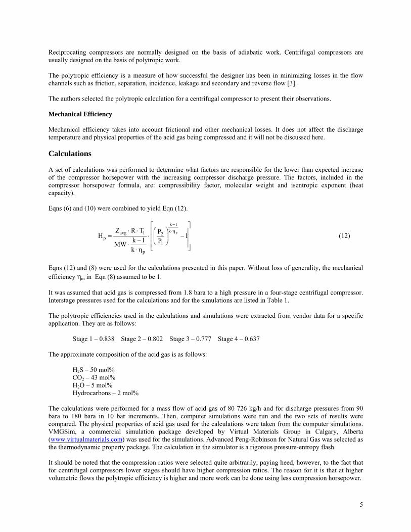
Reciprocating compressors are normally designed on the basis of adiabatic work. Centrifugal compressors are usually designed on the basis of polytropic work. The polytropic efficiency is a measure of how successful the designer has been in minimizing losses in the flow channels such as friction, separation, incidence, leakage and secondary and reverse flow [3]. The authors selected the polytropic calculation for a centrifugal compressor to present their observations. Mechanical Efficiency Mechanical efficiency takes into account frictional and other mechanical losses. It does not affect the discharge temperature and physical properties of the acid gas being compressed and it will not be discussed here. Calculations A set of calculations was performed to determine what factors are responsible for the lower than expected increase of the compressor horsepower with the increasing compressor discharge pressure. The factors, included in the compressor horsepower formula, are: compressibility factor, molecular weight and isentropic exponent (heat capacity). Eqns (6) and (10) were combined to yield Eqn (12).
⎥⎥⎥
⎦
⎤
⎢⎢⎢
⎣
⎡−⎟⎟
⎠
⎞⎜⎜⎝
⎛⋅
η⋅−
⋅
⋅⋅=
η⋅−
1PP
k1kMW
TRZH pk
1k
1
2
p
1avgp (12)
Eqns (12) and (8) were used for the calculations presented in this paper. Without loss of generality, the mechanical efficiency ηm in Eqn (8) assumed to be 1. It was assumed that acid gas is compressed from 1.8 bara to a high pressure in a four-stage centrifugal compressor. Interstage pressures used for the calculations and for the simulations are listed in Table 1. The polytropic efficiencies used in the calculations and simulations were extracted from vendor data for a specific application. They are as follows:
Stage 1 – 0.838 Stage 2 – 0.802 Stage 3 – 0.777 Stage 4 – 0.637 The approximate composition of the acid gas is as follows:
The calculations were performed for a mass flow of acid gas of 80 726 kg/h and for discharge pressures from 90 bara to 180 bara in 10 bar increments. Then, computer simulations were run and the two sets of results were compared. The physical properties of acid gas used for the calculations were taken from the computer simulations. VMGSim, a commercial simulation package developed by Virtual Materials Group in Calgary, Alberta (www.virtualmaterials.com) was used for the simulations. Advanced Peng-Robinson for Natural Gas was selected as the thermodynamic property package. The calculation in the simulator is a rigorous pressure-entropy flash. It should be noted that the compression ratios were selected quite arbitrarily, paying heed, however, to the fact that for centrifugal compressors lower stages should have higher compression ratios. The reason for it is that at higher volumetric flows the polytropic efficiency is higher and more work can be done using less compression horsepower.
Table 1: Interstage pressures used for the calculation of the compression horsepower Stage 1 Stage 2 Stage 3 Stage 4 Suction Pressure bara 1.8 4.6 12.3 33.3 Discharge Pressure bara 5.3 13.0 34.0 90 Compression Ratio 2.94 2.83 2.76 2.70 Suction Pressure bara 1.8 4.6 12.7 35.3 Discharge Pressure bara 5.3 13.4 36.0 100 Compression Ratio 2.94 2.91 2.83 2.83 Suction Pressure bara 1.8 4.7 13.3 38.3 Discharge Pressure bara 5.4 14.0 39.0 110 Compression Ratio 3.00 2.98 2.93 2.87 Suction Pressure bara 1.8 4.8 13.8 40.4 Discharge Pressure bara 5.5 14.5 41.1 120 Compression Ratio 3.06 3.02 2.98 2.97 Suction Pressure bara 1.8 4.9 14.4 43.3 Discharge Pressure bara 5.6 15.1 44.0 130 Compression Ratio 3.11 3.08 3.06 3.00 Suction Pressure bara 1.8 5.1 15.7 47.5 Discharge Pressure bara 5.8 16.4 48.2 140 Compression Ratio 3.22 3.22 3.07 2.95 Suction Pressure bara 1.8 5.3 16.8 50.8 Discharge Pressure bara 6.0 17.5 51.5 150 Compression Ratio 3.33 3.30 3.07 2.95 Suction Pressure bara 1.8 5.4 17.3 54.3 Discharge Pressure bara 6.1 18.0 55.0 160 Compression Ratio 3.39 3.33 3.18 2.95 Suction Pressure bara 1.8 5.5 18.1 57.8 Discharge Pressure bara 6.2 18.8 58.5 170 Compression Ratio 3.44 3.42 3.23 2.94 Suction Pressure bara 1.8 5.7 19.3 61.3 Discharge Pressure bara 6.4 20.0 62.0 180 Compression Ratio 3.56 3.51 3.21 2.94 The compressor horsepower is also affected by the pressure drop across the coolers and valves. It was assumed that the interstage pressure drops are 0.7 bar. Higher pressure drops obviously increase the compressor horsepower.
6
Results The results from the various calculations are listed and compared in Table 2 and Fig. 1. Table 2: Comparison of calculated and simulated compression horsepower
Fig. 1 shows the relationship between the discharge pressure and the compression horsepower. The horsepower curves resemble a power function f(x) = a·xb. Is the rate of the compression horsepower increase the same for all gases? To answer that question a set of calculations was performed for methane compression. Fig. 2 shows the calculated compression horsepower for methane and compares it with the calculated compression horsepower for acid gas.
A curve fit for acid gas and methane curves on Fig. 2 gives the following approximate equations:
Acid Gas curve: 152.02P4613Bhp ⋅=
Methane curve: 217.02P8476Bhp ⋅=
The curves and the equations show that increasing the discharge pressure of acid gas from 90 bara to 180 bara requires only 28% of the horsepower that is required to increase the discharge pressure of methane from 90 bara to 180 bara. The results of the horsepower calculations reveal that the compressor horsepower is a stronger function of the discharge pressure for methane than for acid gas. In other words – the horsepower increase with increasing discharge pressure is less for acid gas than for methane. Let’s now analyze the physical properties of the acid gas to see how they affect the compressor horsepower.
8
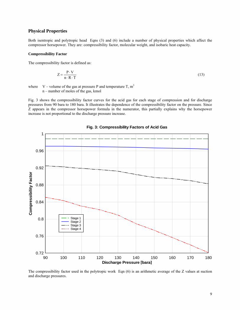
Physical Properties Both isentropic and polytropic head Eqns (3) and (6) include a number of physical properties which affect the compressor horsepower. They are: compressibility factor, molecular weight, and isobaric heat capacity. Compressibility Factor The compressibility factor is defined as:
TRnVPZ⋅⋅
⋅= (13)
where V – volume of the gas at pressure P and temperature T, m3
n – number of moles of the gas, kmol Fig. 3 shows the compressibility factor curves for the acid gas for each stage of compression and for discharge pressures from 90 bara to 180 bara. It illustrates the dependence of the compressibility factor on the pressure. Since Z appears in the compressor horsepower formula in the numerator, this partially explains why the horsepower increase is not proportional to the discharge pressure increase.
Discharge Pressure [bara]
Com
pres
sibi
lity
Fact
or
Fig. 3: Compressibility Factors of Acid Gas
90 100 110 120 130 140 150 160 170 1800.72
0.76
0.8
0.84
0.88
0.92
0.96
1
Stage 1Stage 2Stage 3Stage 4
The compressibility factor used in the polytropic work Eqn (6) is an arithmetic average of the Z values at suction and discharge pressures.
9
Fig. 4 illustrates the differences between the suction and discharge Z factors for the four-stage compression process with the final discharge pressure of 180 bara.
Acid Gas Temperature [°C]
Z Fa
ctor
Fig. 4: Z Factors for the Final Discharge Pressure of 180 bara
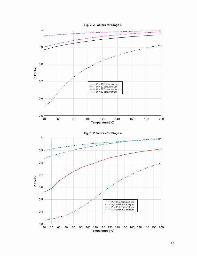
Fig. 4 shows that the Z factor values increase with increasing temperature and decrease with increasing pressure for the range of temperatures and pressures shown in this figure. Figures 5 to 8 compare Z factors of acid gas and methane for each of the four stages of compression for the final discharge pressure of 180 bara. Z factors for acid gas are already presented on Fig. 4 but comparing them with Z factors for methane requires separate graphs to avoid overcrowding the graph with too many curves. For each compression stage, the Z factors for methane are larger than those for acid gas. According to Eqn (6), increasing values of Z factor increase the compression horsepower, which explains higher rate of compression horsepower increase for methane than for acid gas.
Molecular Weight Fig. 9 shows the molecular weight of the acid gas for each stage of compression and for final compressor discharge pressures from 90 bara to 180 bara. The increase of the molecular weight from stage 1 to stage 2 and from stage 2 to stage 3 is due to liquid water dropout in suction scrubbers. The increase of the molecular weight with increasing discharge pressure is due to more liquid water dropout in suction scrubbers. The opposite can be said about methane. The reason lies in the differences in molecular weight of acid gas, methane and water. Lowering the amount of water in acid gas increases its molecular weight. Lowering the amount of water in methane decreases its molecular weight.
Discharge Pressure [bara]
Mol
ecul
ar W
eigh
t
Fig. 9: Molecular Weight of Acid Gas
90 100 110 120 130 140 150 160 170 18037.7
37.8
37.9
38
38.1
38.2
38.3
38.4
38.5
38.6
38.7
38.8
Inlet to Stage 1Inlet to Stage 2Inlet to Stages 3 and 4
Molecular weight appears in the denominator of the compression horsepower equation. Increasing values of the molecular weight slow the increase of the compression horsepower with increasing discharge pressure. The same cannot be said about methane. Since the molecular weight of methane is lower than the molecular weight of water, lowering the amount of water in methane decreases its molecular weight and increases the compression horsepower. This effect, in reality, is small and usually water in the gas is neglected in the compressor design. The effect of molecular weight changes on the rate of increase of the compression horsepower may be negligible, but the molecular weight itself affects the compression horsepower considerably. The reason the compression horsepower for methane is 2.5 to 2.6 times higher than for acid gas is that the molecular weight of acid gas is 2.3 to 2.4 times higher than the molecular weight of methane.
13
Heat Capacity The isobaric heat capacity of a substance (heat capacity at constant pressure) is defined as [2]:
PP T
HC ⎟⎟⎠
⎞⎜⎜⎝
⎛∂∂
= (14)
The isochoric heat capacity of a substance (heat capacity at constant volume) is defined as:
VV T
UC ⎟⎟⎠
⎞⎜⎜⎝
⎛∂∂
= (15)
Definitions (14) and (15) accommodate both the molar and specific heat capacity; the unit of the heat capacity can therefore be kJ/kmol⋅K or kJ/kg⋅K. For an ideal gas, the relationship between heat capacity at constant volume and heat capacity at constant pressure is:
RCC PV −= (16) Since the isochoric heat capacities are so easily calculated from the isobaric heat capacities, they are rarely given in tabulated data. An important reason for obtaining the isochoric heat capacity is that we desire the following quantity:
V
P
CCk = or
RCCkP
P−
= (17)
which, as we have seen, is a quantity used in compressor calculations. The k values used in the calculations are arithmetic average values between suction and discharge conditions. Fig. 10 shows the ideal gas isobaric heat capacity of acid gas.
14
Discharge Pressure [bara]
Cp
[kJ/
kmol
-°C
]
Fig. 10: Ideal Gas Isobaric Heat Capacity of Acid Gas
Isobaric heat capacity Cp of acid gas increases with increasing discharge pressure. Ideal gas heat capacities are independent of the pressure and the increase is due to higher temperatures at discharge pressures. According to Eqn (17), increasing the isobaric heat capacity lowers the k value. This is additionally illustrated on Fig. 10a.
35 40 451.2
1.25
1.3
1.35Fig. 10a: k as function of Cp
Cp
Cp 8.314−
Cp Figures 11 and 12 show the k values for each stage of compression and for final discharge pressures from 90 to 180 bara for acid gas and for methane. Higher k values increase the compression horsepower. On the other hand, decreasing k values with increasing discharge pressures lower the rate of increase of the compression horsepower.
15
Discharge Pressure [bara]
Ave
rage
Isen
trop
ic E
xpon
ent,
k
Fig. 11: Average Isentropic Exponent for Acid Gas
90 100 110 120 130 140 150 160 170 1801.27
1.272
1.274
1.276
1.278
1.28
1.282
Stage 1Stage 2Stage 3Stage 4
Discharge Pressure [bara]
Ave
rage
Isen
trop
ic E
xpon
ent,
k
Fig. 12: Average Isentropic Exponent for Methane
90 100 110 120 130 140 150 160 170 1801.248
1.252
1.256
1.26
1.264
1.268
1.272
Stage 1Stage 2Stage 3Stage 4
16
Eqn (12) used in the calculations of the compression horsepower contains a group of physical properties, which we
called a “Properties Group”:
p
1avg
k1kMW
TRZ
η⋅−
⋅
⋅⋅ and a compression ratio exponent:
pk1kη⋅− , which we called a “k Group”.
1 1.5 20
0.5
1Fig. 13a: k Group as a function of k
k 1−
k 0.838⋅
k 1−
k 0.637⋅
k
The effect of k value on the value of the “k Group” is not obvious at first glance. Fig. 13a shows the “k Group” as a function of k for the first stage and the fourth stage polytropic efficiency. It is a form of a power function and not a linear function. Decreasing k values with increasing discharge pressures (Fig. 11 and Fig. 12) lower the compression horsepower. Fig. 13b shows the k Group for acid gas as a function of the discharge pressure.
Discharge Pressure [bara]
(k-1
)/(kη
p)
Fig. 13b: k Group for Acid Gas - (k-1)/(kηp)
90 100 110 120 130 140 150 160 170 1800.25
0.26
0.27
0.28
0.29
0.3
0.31
0.32
0.33
0.34
Stage 1Stage 2Stage 3Stage 4
The graph shows that except for Stage 4 the values of the k Group decrease with increasing discharge pressures. This is in agreement with Fig. 11. With increasing discharge pressure, however, interstage compression ratios increase. This causes the compression horsepower to increase. Decreasing k Group values only slow down the rate of increase of the compression horsepower values.
17
Fig 13c shows the effect of k values on the compressor horsepower for the first stage and fourth stage polytropic efficiency and for the compression ratio of 3. The dependent variable on Fig. 13c constitutes part of the polytropic head Eqn (12), which in turn is part of the compression horsepower equation. Again, the decreasing k value with increasing compressor discharge pressure lowers the compression horsepower. It is the increasing compression ratio with increasing discharge pressure that produces a net increase of the compression horsepower.
1.26 1.281.25
1.3
Fig. 13c: Effect of k value on HP
1
k 1−
k 0.838⋅⎛⎜⎝
⎞⎟⎠
3
k 1−k 0.838⋅ 1−
⎛⎜⎝
⎞⎟⎠⋅
1
k 1−
k 0.637⋅⎛⎜⎝
⎞⎟⎠
3
k 1−k 0.637⋅ 1−
⎛⎜⎝
⎞⎟⎠⋅
k Fig. 14 shows Properties Group values as a function of the discharge pressure.
Discharge Pressure [bara]
PG [k
J/kg
]
Fig 14: Properties Group (PG) for Acid Gas
90 100 110 120 130 140 150 160 170 180150
160
170
180
190
200
210
220
230
240
250
260
270
Stage 1Stage 2Stage 3Stage 4
18
Looking at the Properties Group
p
1avg
k1kMW
TRZ
η⋅−
⋅
⋅⋅ and at Figures 3, 9 and 13b, one can notice that changes in molecular
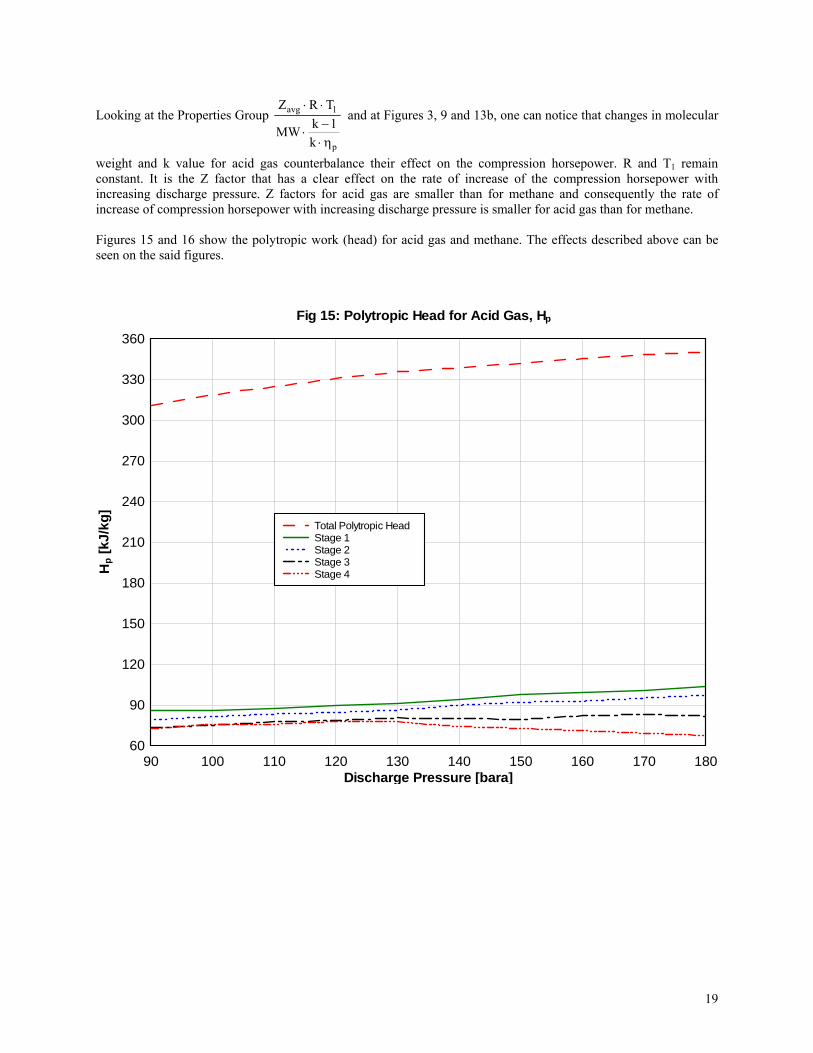
weight and k value for acid gas counterbalance their effect on the compression horsepower. R and T1 remain constant. It is the Z factor that has a clear effect on the rate of increase of the compression horsepower with increasing discharge pressure. Z factors for acid gas are smaller than for methane and consequently the rate of increase of compression horsepower with increasing discharge pressure is smaller for acid gas than for methane. Figures 15 and 16 show the polytropic work (head) for acid gas and methane. The effects described above can be seen on the said figures.
Discharge Pressure [bara]
Hp
[kJ/
kg]
Fig 15: Polytropic Head for Acid Gas, Hp
90 100 110 120 130 140 150 160 170 18060
90
120
150
180
210
240
270
300
330
360
Total Polytropic HeadStage 1Stage 2Stage 3Stage 4
19
Discharge Pressure [bara]
Hp
[kJ/
kg]
Fig 16: Polytropic Head for Methane, Hp
90 100 110 120 130 140 150 160 170 180160
240
320
400
480
560
640
720
800
880
960
Total Polytropic HeadStage 1Stage 2Stage 3Stage 4
Discharge Temperature Calculations Compressor discharge temperatures T2 were calculated using the following equation:
pηk1k
1
212 P
PTT
⋅−
⎟⎟⎠
⎞⎜⎜⎝
⎛⋅= (18)
Table 3 and Fig. 17 show the calculated discharge temperatures for each compression stage and each final discharge pressures from 90 bara to 180 bara. Interstage and final discharge temperatures increase with increasing pressure ratios. The discharge temperatures of the fourth stage of compression for the final pressures 140 bara and up go down. The reason is that the fourth stage compression ratios were lowered to avoid further increase in discharge temperature much above 200°C. Multistage compressors use interstage cooling to lower the gas temperature and the head. Lower head means lower speed or a smaller compressor. At a lower temperature, the specific volume is smaller. For a given mass flow it leads to a smaller compressor size. If the same pressure ratio is required, lowering the head saves the horsepower. Compression with intercooling approximates an isothermal thermodynamic process.
20
Table 3: Discharge temperatures from acid gas compression calculations Disch. P Discharge Temperatures from VMGSim Discharge Temp. Calculated with Eqn (18)
bara °C °C Stage 1 Stage 2 Stage 3 Stage 4 Stage 1 Stage 2 Stage 3 Stage 4 90 147.9 144.0 146.4 191.9 147.2 142.7 143.7 196.1 100 147.9 147.4 149.4 198.3 147.2 146.0 146.5 203.2 110 149.9 149.9 153.5 199.4 149.2 148.5 150.4 205.4 120 151.9 151.5 155.4 203.6 151.2 150.0 152.2 210.6 130 153.8 153.8 158.6 204.1 153.1 152.2 155.1 212.3 140 157.6 158.7 159.4 199.7 156.9 157.0 155.6 209.5 150 161.3 161.8 159.4 198.4 160.5 160.0 155.4 209.9 160 163.1 162.9 163.9 196.2 162.3 161.0 159.6 209.6 170 164.9 165.8 166.0 193.7 164.1 163.9 161.6 209.4 180 168.4 168.9 165.5 191.0 167.6 166.8 160.8 209.3 The differences between calculated and simulated discharge temperatures increase with increasing stage number and with increasing discharge pressure. For 90 bara discharge pressure the difference for Stage 1 is –0.45% (-0.7°C) and for 180 bara and Stage 4 the difference is 9.59% (18.3°C). The error increases with increasing k values. The big difference in discharge temperatures between lower stages of compression and Stage 4 is caused by higher fourth stage suction temperature. It has to be higher to avoid acid gas condensation.
Discharge Pressure [bara]
Dis
char
ge T
empe
ratu
re [°
C]
Fig. 17: Discharge Temperatures for Acid Gas
90 100 110 120 130 140 150 160 170 180130
140
150
160
170
180
190
200
210
220
Stage 1Stage 2Stage 3Stage 4
21
Effect of Impurities Acid gas impurities tend to broaden acid gas phase envelope. This affects compressor discharge temperature and pressure because the interstage temperature to which acid gas can be cooled must be increased to avoid acid gas condensation. Perhaps the most important impurity in an acid gas stream beside water is methane; methane is significantly more volatile than the acid gas components. Thus, it tends to broaden the phase envelope. In the design and operation of an acid gas compression scheme, it is important to avoid entering the phase envelope. Besides, the presence of methane reduces the density of the gas. Since the injection pressure is directly related to the density, the presence of the methane increases the required injection pressure and hence increases the required compressor power. The calculations and the analysis of methane properties prove that the compressor horsepower increases with increasing concentration of methane in acid gas. Conclusions Physical properties of acid gas are responsible for the phenomenon of lowering of compression horsepower increase with increasing discharge pressure. The strongest effect on this has the compressibility factor and to a lesser degree the isentropic exponent (heat capacity). Another reasons for non-linear relationship between the discharge pressure and the compressor horsepower Bhp is the non-linear function Bhp = f(k). References 1. Engineering Data Book, SI Version, 12th Ed., Gas Processors Suppliers Association, Tulsa, 2004. 2. Smith, J.M., Van Ness, H.C., Abbott, M.M., “Introduction to Chemical Engineering Thermodynamics”, 7th Ed.,