Received: 17 May 2018 Revised: 4 December 2018 Accepted: 21 February 2019
DOI: 10.1002/rnc.4531
R E S E A R C H A R T I C L E
Observers and observability for uncertain nonlinearsystems: A necessary and sufficient condition
Wenyan Bai1 Sen Chen2,3 Yi Huang2,3 Bao-Zhu Guo2,3,4 Ze-Hao Wu4
1Beijing Aerospace Automatic ControlInstitute, Beijing, China2Key Laboratory of System and Control,Academy of Mathematics and SystemsScience, Chinese Academy of Sciences,Beijing, China3School of Mathematical Sciences,University of Chinese Academy ofSciences, Beijing, China4School of Mathematics and Big Data,Foshan University, Foshan, China
CorrespondenceZe-Hao Wu, School of Mathematics andBig Data, Foshan University, Foshan528000, China.Email: [email protected]
Funding informationNational Natural Science Foundation ofChina, Grant/Award Number: 61603365,61873260, and 11801077; Natural ScienceFoundation of Guangdong Province,Grant/Award Number: 2018A030310357;Project of Department of Education ofGuangdong Province, Grant/AwardNumber: 2017KTSCX191 and2017KZDXM087
Summary
In this paper, observers and observability for uncertain nonlinear systems aresystematically discussed. It is shown that for the convergence of a large classof observers, featured with the augment state to estimate the uncertainty, itrequires not only the observability condition for the augment matrix pair but,more importantly, requires a structural condition first proposed in this paper.Furthermore, it is demonstrated that the combination of this structural condi-tion and the observability of the augment matrix pair is a necessary and sufficientcondition for the convergence of the observers and the observability of the origi-nal uncertain nonlinear systems. This implies that both the structural conditionand the observability condition of the augment matrix pair reveal essentialfeature of the observing problems for uncertain nonlinear systems. In addi-tion, for unobservable uncertain nonlinear systems, which do not satisfy thisnecessary and sufficient condition, the biased estimation error is explicitly pre-sented, which can be used to evaluate the estimation performance of this classof observers. The numerical simulations for three typical examples are carriedout to validate our theoretical analysis.
KEYWORDS
convergence of the observer, extended state observer, observers, uncertain nonlinear systems
1 INTRODUCTION
Uncertainties, including but not limited to external disturbances, unmodeled dynamics, and parameter perturbations,are ubiquitous in industrial systems and often bring adverse effects on performance and even stability of engineeringsystems.1-5 For this reason, ensuring normal operation for a control system under various uncertainties becomes a centralissue in control theory. In recent years, the control approaches with estimation/compensation of uncertainty to forcethe system to satisfy desired performance have been substantially developed for the control of uncertain systems.6-16 Theeffectiveness of such control strategies lies in large part in the observer design, which is used not only to recover the statebut also the uncertainty. In this sense, the observer design has become a bedrock for the control of uncertain systems.
During the past decades, several classes of observers, including but no limited to extended state observer (ESO),17,18
proportional-integral observer (PIO)23 and disturbance observer (DO)6 have been proposed to estimate state or uncer-tainty. Although using different names, these observers are based on the similar idea: expanding the state in the observer
to include the uncertainty estimation. This state augment design has been shown as an effective way for estimating uncer-tainties in practice. Substantial researches have been produced to analyze these classes of observers theoretically. Theconvergence of nonlinear ESO with matched uncertainty has been studied in the work of Guo and Zhao.11,18 Under theassumption that the nonlinear system is minimum phase, Freidovich and Khalil19 prove that the closed-loop system basedon the EHGO-based controller is stable. Hammouri and Tmar24 study a necessary and sufficient condition for the exis-tence of UIO, and the stability condition of UIO is also presented. For bounded external disturbance, stability of GESOfor systems with mismatched disturbances has been studied in the work of Li et al.22 Considering discrete-time nonmin-imum phase systems, it is shown that the estimation errors of the system state and unknown disturbance from PIO canbe constrained in a small bounded region.25 The global exponential stability of the estimation error from nonlinear DOhas been investigated in the work of Chen.6
Although some observers have been studied thoroughly from different perspectives, the theoretical analyses may havethe following two limitations:
• The structure of uncertain systems is limited to a special form. For instance, ESO and EHGO are constructed for thoseuncertain systems that have cascade form and control matched uncertainty17,19;
• The assumptions on large-time behavior of uncertainties are conservative. For instance, the asymptotic stability of theestimation errors of GESO and DO are proved under the assumption that the uncertainty converges to a constant astime goes to infinity.6,22
However, in real physical plants, the uncertainties may affect the system from each channel, which can be mismatchedwith the control input. Moreover, the uncertainties might be composed of the time-varying external disturbances andlinear/nonlinear unknown dynamics with respect to system states. To meet the requirement of engineering applications,the detailed analysis of observers for uncertain nonlinear systems under a more general framework becomes significantboth theoretically and practically.
A fundamental problem motivates this investigation is: what kinds of uncertainties can be estimated by observer forgeneral uncertain nonlinear systems?
We are therefore focused ourselves to uncertainty observing problem for general uncertain nonlinear systems in thispaper. Firstly, we analyze estimation performance of observers for a large class of uncertain nonlinear systems. The observ-ability for uncertain nonlinear systems is thus defined, which was neglected in previous studies. Secondly, we try to revealthe essential nature of the observability for uncertain nonlinear systems. The main contributions of this paper consist offour main points: a) The properties of the observers for a general class of uncertain nonlinear systems are rigorously ana-lyzed and a structural condition, which is proved to be the essential condition to ensure the convergence of the observers,is proposed in this paper; Specially, the performance of observers for uncertain nonlinear systems is quantitativelyanalyzed; b) The combination of the structural condition proposed in this paper and the observability of the augmentmatrix pair is proved to be a necessary and sufficient condition for the observers to be convergent; c) The observability foruncertain nonlinear systems is defined. The combination of the structural condition and the observability of the augmentmatrix pair is proved to be a necessary and sufficient condition for the uncertain systems to be observable. In particular,an algebraic criterion of the observability for uncertain nonlinear systems is presented; d) For unobservable uncertainnonlinear systems, the biased estimation error of the observers is quantitatively given in this paper, which can be used toevaluate the estimation performance of the observers.
The paper is organized as follows. In Section 2, the observation problem and the observers for a large class of uncertainnonlinear systems are introduced. In Section 3, the properties of the observers are analyzed and a necessary and sufficientcondition for convergence of the observers is presented. In Section 4, the condition in Section 3 is also proved to be nec-essary and sufficient for observability of uncertain nonlinear systems. Finally, in Section 5, some numerical experimentsare performed to validate the theoretical results.
The following notations are used throughout the paper. TheRn represents the n-dimensional Euclidean space andRn×m
stands for the space of real n × m-matrices; C− denotes the left-half complex plane; for a vector or matrix Y, Y⊤ denotes itstranspose; for a square matrix Y, Y−1 denotes its inverse matrix; for a square matrix Y, 𝜎(Y) denotes the set of eigenvaluesof Y; In×n denotes the n × n unit matrix; 𝜆min(Y ) and 𝜆max(Y ) represent the minimal and maximal eigenvalues of thesymmetric real matrix Y, respectively; ||Y|| denotes the Euclidean norm of the vector Y and the corresponding inducednorm when Y is a matrix; Cs(Rn;R) denotes the set of all continuous differentiable functions from Rn to R up to s-order;for any given function g, g( j) denotes its j-order total differentiation with respect to t, and specially f ( j) means d𝑗𝑓 (X(t),d(t),t)
dt𝑗for the unknown function f(·) in system (1) in the beginning of next section for simplicity.
2962 BAI ET AL.
2 PROBLEM FORMULATION
In this paper, we consider a class of uncertain nonlinear systems described as follows:{ .X(t) = AoX(t) + buu(t) + bd𝑓 (X(t), d(t), t),𝑦(t) = cX(t),
(1)
where X(t) ∈ Rn is the state vector, 𝑦(t) ∈ R is the measured output, u(t) ∈ R is the control input, d(t) ∈ R is the externaldisturbance, and 𝑓 ∈ Cn(Rn+1 ×[0,∞);R) is an unknown function representing the uncertainty, which contains externaldisturbance d(t), unmodeled dynamics, and parameter perturbations. Ao ∈ Rn×n, bu ∈ Rn, bd ∈ Rn, c ∈ R1×n are knownconstant matrix and vectors. It is suppose without loss of generality that all bu, bd, c are nonzero.
We first specify some assumptions about system (1) in what follows. The following Assumption 1 is about the state X(t),the input u(t), and the external disturbance d(t).
Assumption 1. The state X(t) and the input u(t) of system (1) are supposed to be bounded
supt≥0
||X(t)|| + supt≥0
|u(t)| ≤ M1; (2)
and the external disturbance d(t) satisfies
supt≥0
||(d(t), .d(t), … , d(n)(t))|| ≤ M2, (3)
where Mi(i = 1, 2) are some positive constants.
The following Assumption 2 is about the unknown function f(·).
Assumption 2. There exists a nonnegative continuous function 𝜍 ∈ C(Rn+1; [0,∞)), such that for any functiongj ∈ ∇( j)f( j = 2, … ,n),
where ∇f and ∇( j)f represent the gradient of f and the finite set of all j-order partial derivatives of f with respect to itsarguments, respectively.
Remark 1. It is significant to emphasize that both Assumption 1 and Assumption 2 are essentially to ensure theboundedness of f ( j)(j = 1, 2, … ,n). It also should be noticed that the boundedness requirement for the state X(t) inAssumption 1 aims for estimating the state-dependent uncertainty f(X(t), d(t), t), so that this boundedness assumptioncan be removed in the case that the uncertainty function is state independent. Moreover, the state could be boundedin many practical control systems such as those for faults diagnosis.26 Finally, since the observer is usually designedfor feedback purpose, we can use observer-based feedback to make the state be bounded.9,11,12,18
Remark 2. Assumption 2 is about the “growth” requirement of the time-varying unknown function f(X, d, t) withrespect to (X, d), which is reasonable as stated in Remark 1. However, if the unknown function f(X, d, t) is time indepen-dent, the Assumption 2 can be removed since in this case the left-hand side of (4) is always a nonnegative continuousfunction with respect to (X, d) and ∇( j)f is just a finite set for each j = 1, 2, … ,n.
We point out that many physical systems can be modeled by system (1). Examples can be found from robotic systems,27
DC-DC converter,28 flight systems,29 among many others (see, eg, the work of Xue et al30). For the control of system (1),there is a widely used method that performs two steps.15 One step is to estimate the uncertainty through observe andthe other is to compensate for the uncertainty in the feedback loop. The central strategy of this approach is the distur-bance/observer/estimator, which provides an online estimation of the disturbance or uncertainty such as ESO, EHGO,PIO, and GESO.
General observers of variable augment design to estimate the uncertainty are of the following form:[ .X(t).𝑓 (t)
]= A
[X(t)𝑓 (t)
]+ Buu(t) + L
(𝑦(t) − C
[X(t)𝑓 (t)
]), (5)
BAI ET AL. 2963
where X(t) ∈ Rn and 𝑓 (t) ∈ R are the estimates of the state X(t) and the lumped uncertainty f(X(t), d(t), t), respectively;A, Bu, and C are the following extended matrices
A =[
Ao bd0 0
], Bu =
[bu0
], C = [ c 0 ], (6)
and L ∈ Rn+1 is the observer gain vector to be designed.In fact, the observer (5) is a general form for uncertain systems in the sense that all ESO, EHGO, PIO, and GESO are
special cases of (5), which can be summarized from the following two aspects.
a) Both ESO and EHGO17,19 are designed for special integral cascade systems, where
Ao =⎡⎢⎢⎢⎣
0 1 … 0⋮ ⋱ ⋱ ⋮0 … 0 10 … … 0
⎤⎥⎥⎥⎦ , bd =⎡⎢⎢⎢⎣
0⋮01
⎤⎥⎥⎥⎦ , bu =⎡⎢⎢⎢⎣
0⋮01
⎤⎥⎥⎥⎦ , c = [ 1 0 … 0 ], (7)
which assumes that the relative degree from the control input to the controlled output is n and the lumped uncertaintyis matched with the control input;
b) The GESO and PIO22,23 are for general Ao, bd, bu, c, the lumped uncertainty is, however, commonly assumed to beultimately steady, ie, limt→∞𝑓
(1) = 0, which ensures asymptotically convergence of the estimation error. This paperwill further study the transient performance of the observer (5) without this ultimately steady assumption.
To analyze the performance of observer (5), we start from the estimation error:
𝜂(t) =[
X(t)𝑓 (X(t), d(t), t)
]−[
X(t)𝑓 (t)
]. (8)
It is seen that the estimation error is governed by
.𝜂(t) = (A − LC)𝜂(t) + Bd𝑓
(1), (9)
where Bd =[
0n×11
]. To achieve asymptotically unbiased estimation 𝜂(∞) = 0, the observability of (A,C) is a basic
condition, which is commonly used in previous studies.17,19,22,23 This is because if (A,C) is observable, A − LC can bedesigned to be Hurwitz by tuning L. Solve the error Equation (9) to obtain
𝜂(t) = e(A−LC)t𝜂(0) + ∫t
0e(A−LC)(t−s)Bd𝑓
(1)ds. (10)
It is seen that when (A,C) is observable, e(A−LC)t can decay as fast as desired by choosing the appropriate gain matrix Lfrom the pole assignment. Thus, if the uncertainty f(·) is a constant function, ie, f (1) ≡ 0, it follows from (7) and (10) that𝜂(∞) = 0. Therefore, it is often assumed that the uncertainty is ultimately steady, ie, limt→∞𝑓
(1) = 0 to ensure asymp-totically unbiased estimation.22,23 However, if f(·) is not a constant function, ie, f (1) ≢ 0, there is not necessarily existinga gain vector L to achieve asymptotically unbiased estimation even if (A,C) is observable, which can be easily seen fromsome simple counter examples, such as example 2 in Section 5.1 later. It is natural that some additional conditions aboutbd in system (1), which demonstrates the position of the uncertainty f, should be required to ensure the asymptoticallyunbiased estimation of the observer (5).
Actually, for general uncertainty f(·) satisfying Assumption 2, if (A,C) is observable and Assumptions 1 and 2 aresatisfied, the following proposed structural condition:
cbd = 0, cA0bd = 0, … , cAn−20 bd = 0, cAn−1
0 bd ≠ 0 (11)
will be proved to be not only a sufficient condition but also a necessary one to guarantee that there always exists a gainvector L such that the observer (5) is convergent, which is presented in Theorem 2 in the next section. Specially, if weonly consider the sufficient condition for the convergence of the observer (5), we can replace Assumptions 1 and 2 by thefollowing weaker Assumption 3, then (A,C) is observable and condition (11) can insure that there always exists a gainvector L such that the observer (5) is convergent, which is shown in Proposition 1 in the next section.
2964 BAI ET AL.
3 CONVERGENCE OF THE OBSERVER
Before analyzing the performance of the observer (5), we first give two essential properties, which make the observerfeasible. The observer (5) is said to be convergent if the following conditions (P1) and (P2) are satisfied.
(P1). The observer is interiorly stable, ie, 𝜎(A − LC) ⊂ C−.(P2). The estimation accuracy of the observer can be adjusted by 𝜎(A − LC), that is to say, for any T > 0 and any
𝜀 ∈ (0, 1], there exists L′ such that 𝜎(A − L′C) = 1𝜀𝜎(A − LC) and||𝜂(t)|| ≤ Γ𝜀,∀ t > T, (12)
where 𝜂(t) is defined as in (8) and Γ is a constant independent of 𝜀.
As discussed in Section 2, (P1) is a basic property for the observer to be practicable. (P2) means that the estimationerror of the observer (5) can be eventually unbiased ∶ lim𝜀→0||𝜂(t)|| = 0 by tuning the observer gain L′ in every time.Actually, unlike properties analyzed in general observers, (P2) ensures not only the ultimate performance but also, moreimportantly, the transient performance. Since (P1) and (P2) are preconditions for the observer (5) to be convergent, it issignificant to discuss under what conditions or for what kind of uncertainties, the observer can satisfy both (P1) and (P2).
According to the dynamics of the estimation error (9), it is difficult or even impossible to find analytically the estimationerror for general A,C, and f. Thus, we will first transform (9) into a special form that is more easy to be analyzed. The keysteps of this transform can be summarized as follows. First, since the observability of (A,C) is the prime condition for thefeasibility of observer, we always assume that (A,C) is observable. In this case, there is an (n + 1) × (n + 1) invertiblematrix
S ≜⎡⎢⎢⎢⎢⎣
CCACA2
⋮CAn
⎤⎥⎥⎥⎥⎦=
⎡⎢⎢⎢⎢⎣c 0
cA0 cbdcA2
0 cA0bd⋮ ⋮
cAn0 cAn−1
0 bd
⎤⎥⎥⎥⎥⎦(13)
such that (A,C) can be changed into the observable canonical form
SAS−1 = A, CS−1 = C, (14)
where
A =⎡⎢⎢⎢⎣
0 1 … 0⋮ ⋮ ⋱ ⋮0 0 … 1[
cAn+10 cAn
0 bd]
S−1
⎤⎥⎥⎥⎦(n+1)×(n+1)
, C =[
1 0 … 0]
1×(n+1). (15)
Then, the estimation error (9) can be reformulated as.��(t) = (A − LC)��(t) + Bd𝑓
(1), (16)
where we set��(t) = S𝜂(t), L = SL, Bd = SBd. (17)
We can see that the if we only consider the first term of the right-hand side of (16), it has been the estimation error of theobservable canonical form. We focus only on the second term Bd𝑓
(1). Let
Δ =
⎡⎢⎢⎢⎢⎣0 … 00 … 0
cbd … 0⋮ ⋱ ⋮
cAn−20 bd … cbd
⎤⎥⎥⎥⎥⎦[
𝑓 (1)
⋮𝑓 (n−1)
]. (18)
It is verified that.Δ = AΔ − Bd𝑓
(1) + F, (19)
where
F = −[
0n×11
] [cAn−1
0 bd … cbd] [ 𝑓 (1)
⋮𝑓 (n)
]+[
0n×11
] [cAn+1
0 cAn0 bd
]S−1Δ. (20)
BAI ET AL. 2965
Since CΔ = 0, (19) becomes .Δ = (A − LC)Δ − Bd𝑓
(1) + F. (21)Denote
𝜂o = �� + Δ. (22)It then follows from (16) and (21) that
.𝜂o = (A − LC)𝜂o + F. (23)
From the discussion above, we can see that the error Equation (9) is reformulated as (23) in the observable canonicalform. The convergence of system (23) is presented in the succeeding Lemma 1.
Lemma 1. Suppose that F defined in (20) is bounded. Then, there exists an (n + 1)-dimensional vector L such thatsystem (23) satisfies both (P1) and (P2).
Proof. Since (A, C) is observable with both A and C defined in (15), for any {��1, ��2, … , ��n} ⊂ C−1, there exists an(n + 1)-dimensional vector L0 such that
A − L0C = P0Λ0P−10 , (24)
where
Λ0 =
[��1
⋱��n+1
],
P−10 =
⎡⎢⎢⎢⎢⎢⎢⎢⎢⎢⎣
��n1 −
n+1∑i=2
ai��i−21 ��n−1
1 −n+1∑i=3
ai��i−31 … ��1 − an+1 1
��n2 −
n+1∑i=2
ai��i−22 ��n−1
2 −n+1∑i=3
ai��i−32 … ��2 − an+1 1
⋮ ⋮ ⋱ ⋮ ⋮
��nn+1 −
n+1∑i=2
ai��i−2n+1 ��n−1
n+1 −n+1∑i=3
ai��i−3n+1 … ��n+1 − an+1 1
⎤⎥⎥⎥⎥⎥⎥⎥⎥⎥⎦,
[a1, … , an+1] ≜ [cAn+1
0 cAn0 bd
]S−1.
When we replace Λ0 with 1𝜀Λ0 (𝜀 ∈ (0, 1]) in (24), there also exists an (n + 1)-dimensional vector L such that
A − LC = P[1𝜀Λ0
]P−1, (25)
where P−1 = P−10 T with
T = T−1a
⎡⎢⎢⎢⎣1
𝜀n+11𝜀n
⋱1
⎤⎥⎥⎥⎦Ta (26)
and
Ta =⎡⎢⎢⎢⎣
1 0 … 0−an+1 ⋱ ⋱ ⋮⋮ ⋱ 1 0
−a2 … −an+1 1
⎤⎥⎥⎥⎦ . (27)
The observe error Equation (23) becomes therefore
.𝜂0 = T−1P0
⎡⎢⎢⎢⎣��1𝜀
⋱��n+1
𝜀
⎤⎥⎥⎥⎦P−10 T𝜂0 + F. (28)
Denote𝜗 = T𝜂0. It follows from (24)-(28) that.𝜗 = 1
𝜀(A − L0C)𝜗 + TF. (29)
Since TF = F, (29) becomes.𝜗 = 1
𝜀(A − L0C)𝜗 + F. (30)
2966 BAI ET AL.
Since A − L0C is Hurwitz, there is an (n + 1) × (n + 1) positive definite matrix Q such that
(A − L0C)⊤Q + Q(A − L0C) = −I(n+1)×(n+1). (31)
Let V = 𝜗⊤Q𝜗, which satisfies𝜆min(Q)‖𝜗‖2 ≤ V ≤ 𝜆max(Q)||𝜗||2,
and hence.
V =(1𝜀(A − L0C)𝜗 + F
)⊤
Q𝜗 + 𝜗⊤Q(1𝜀(A − L0C)𝜗 + F
)≤ −1
𝜀𝜗⊤𝜗 + 1
2𝜗⊤𝜗 + 2||QF||2
≤ −1𝜀− 1
2
𝜆max(Q)V + 2||Q||2||F||2.
(32)
Furthermore, since F is bounded, there exists a positive constant C1 such that 2||Q||2||F||2 ≤ C1. This, togetherwith (32), yields
V(t) ≤ e−( 1
𝜀− 1
2 )𝜆max (Q) tV(0) + C1 ∫
t
0e
−( 1𝜀− 1
2 )𝜆max (Q) (t−s)ds. (33)
Since 0 < 𝜀 ≤ 1, we then have
V(t) ≤ e−1
2𝜆max (Q)𝜀 tV(0) + C1 ∫t
0e
−12𝜆max (Q)𝜀 (t−s)ds
≤ e−1
2𝜆max (Q)𝜀 tV(0) + 2𝜆max(Q)C1𝜀.
(34)
In addition, for any given T > 0, there exists a positive constant C2 independent of 𝜀 such that
e−1
2𝜆max (Q)𝜀 tV(0) ≤ C2𝜀, ∀ t ∈ [T,∞). (35)
Let 𝛾 = C2 + 2𝜆max(Q)C1. Then, for any t ≥ T,V ≤ 𝛾𝜀. (36)
This follows that ||𝜂0||2 = ||T−1𝜗||2 ≤ ||T−1||2 1𝜆min(Q)
V ≤ Γ𝜀, ∀ t ∈ [T,∞), (37)
where Γ ≜ ||T−1||2𝜆min(Q)
𝛾 is a constant independent of 𝜀.
By Lemma 1, the capability of observer (5) is demonstrated in the succeeding Theorem 1.
Theorem 1. For the observer (5), if (A,C) is observable and Assumptions 1 and 2 are satisfied, then there exists an(n + 1)-dimensional vector L such that the property (P1) is satisfied; in addition, for any 𝜀 ∈ (0, 1] and T > 0, whenthe gain vector L∗ is chosen such that 𝜎(A − L∗C) = 1
𝜀𝜎(A − LC), it holds
||𝜂(t) + S−1Δ||2 ≤ Γ𝜀,∀ t > T, (38)
where Γ is a constant independent of 𝜀 and 𝜂(t), S, Δ are defined as those in (8), (13), (18), respectively.
Proof. Since Assumptions 1 and 2 are satisfied, we can easily show by a computation that f ( j)( j = 1, 2, … ,n) arebounded. It follows from (20) that F is bounded. By Lemma 1, there exists an (n + 1)-dimensional gain vector L suchthat the estimation error system (23) satisfies both (P1) and (P2). Furthermore, since
SAS−1 = A,CS−1 = C, L = SL, (39)
which is specified in (14) and (17), we have
S(A − LC)S−1 = A − LC, (40)
which means that𝜎(A − LC) = 𝜎(A − LC). (41)
It then follows from Lemma 1 that for any 𝜀 ∈ (0, 1] and T > 0, there exists a gain vector L such that (P1) is satisfied,and ||𝜂(t) + S−1Δ||2 ≤ Γ𝜀,∀ t > T, (42)
BAI ET AL. 2967
for some 𝜀-independent constant Γ when we choose the gain vector L∗ such that 𝜎(A − L∗C) = 1𝜀𝜎(A − LC). This
completes the proof of the theorem.
Theorem 1 shows that the estimation error (𝜂(t) + S−1Δ) can be tuned as small as possible by the observer gain L∗.Moreover, (𝜂(t) + S−1Δ) will converge to zero with the eigenvalues of 𝜎(A − L∗C) tending to negative infinity. Since S−1Δdepends on the uncertainty f(·) and the structure of the original system (1), it cannot be adjusted by the observer gain L∗,which is therefore regarded as a biased estimation of the observer (5).
Theorem 1 is significant in the sense that it gives a quantitative estimation error of the observer (5). To achieve unbiasedestimations, S−1Δ should be a zero vector. From this fact, condition (11) specified in last section is considered as not onlya sufficient condition but also a necessary one for the convergence of the observer (5), which is shown in the followingTheorem 2.
Theorem 2. For the observer (5), suppose that (A,C) is observable and Assumptions 1 and 2 are satisfied. Then, therealways exists an (n + 1)-dimensional gain vector L such that the observer (5) is convergent if and only if condition (11) issatisfied.
Proof. Sufficiency: Since (A,C) is observable, there exists an (n + 1)-dimensional gain vector L such that (P1) issatisfied. If condition (11) is satisfied, from (18), we have Δ ≡ 0. It then follows from Theorem 1 that (P2) holds.
Necessity: Suppose that (P1) and (P2) are satisfied. Then, for any 𝜀 ∈ (0, 1] and T > 0, there exists an(n + 1)-dimensional gain vector L such that 𝜎(A−LC) ⊂ C−, and when we choose the gain L′ such that 𝜎(A−L′C) =1𝜀𝜎(A − LC), we have ||𝜂(t)|| ≤ Γ1𝜀,∀ t > T, (43)
for some 𝜀-independent constant Γ1. Suppose that there is an integer 0 ≤ i ≤ n − 2 such that
cAi0bd ≠ 0,
which yields Δ ≢ 0 for the uncertainty f satisfying f (1) ≢ 0.Since (A,C) is observable and Assumptions 1 and 2 are satisfied, it follows from Theorem 1 that||𝜂(t) + S−1Δ|| ≤ Γ2𝜀,∀ t > T, (44)
for some 𝜀-independent constant Γ2 with the choice of the gain L′. Now,||S−1Δ|| − ||𝜂(t)|| ≤ ||𝜂(t) + S−1Δ|| ≤ Γ2𝜀, (45)
which yields ||𝜂(t)|| ≥ ||S−1Δ|| − Γ2𝜀. (46)
It is easy to see that there exists 𝛾 > 0 such that 𝜃∗ ≜ mint∈[T,T+𝛾]||S−1Δ|| > 0, and we suppose that 0 < 𝜀 <
min{ 𝜃∗
2Γ2,
𝜃∗
3Γ1, 1}. This, together with (46), yields
||𝜂(t)|| ≥ 𝜃∗
2,∀ t ∈ [T,T + 𝛾], (47)
which contradicts with (43). Therefore,cAi
0bd = 0, 0 ≤ i ≤ n − 2. (48)
In addition, since (A,C) is observable, S is nonsingular. Thus, we have cAn−10 bd ≠ 0. This shows condition (11) finally.
Theorem 2 gives the necessary and sufficient condition (11), which is about the system structure for convergence of theobserver (5). It should be noted that the integral cascade system, which is widely discussed in ESO and EHGO, definitelysatisfies (11). This is the reason why ESO and EHGO show good estimation performance for uncertain systems.
The Assumptions 1 and 2 in Theorem 2 can be replaced by the following weaker Assumption 3 as a sufficient conditionabout the unknown function f to guarantee the convergence of the observer (5), which is substantially required for theboundedness of f (1).
Assumption 3. The state X(t) and the input u(t) of system (1) are supposed to be bounded in the sense that
supt≥0
||X(t)|| + supt≥0
|u(t)| ≤ M1, (49)
2968 BAI ET AL.
and the external disturbance d(t) satisfiessupt≥0
||(d(t), .d(t))|| ≤ M2, (50)
where Mi(i = 1, 2) are some positive constants;There exists a nonnegative continuous function 𝜍 ∈ C(Rn+1; [0,∞)), such that
|𝑓 (X , d, t)| + ‖∇𝑓 (X , d, t)‖ ≤ 𝜍(X , d),∀ t ∈ [0,∞),X ∈ Rn, d ∈ R. (51)
Proposition 1. Suppose that (A,C) is observable, condition (11) and Assumption 3 are satisfied. Then, there exists an(n + 1)-dimensional gain vector L such that the observer (5) is convergent.
Proof. Since condition (11) is satisfied, it follows from (20) that
F = −[
0n×11
]cAn−1
0 bd𝑓(1). (52)
Since Assumption 3 is satisfied, a direct computation easily shows that f (1) is bounded and then F is bounded. Similarto the proof of Theorem 1, we can conclude that there exists an (n + 1)-dimensional vector L such that (P1) is satisfied.Besides, for any 𝜀 ∈ (0, 1] and T > 0, ||𝜂(t) + S−1Δ|| ≤ Γ𝜀,∀ t > T, (53)provided we choose the gain matrix L so that 𝜎(A−LC) = 1
𝜀𝜎(A−LC). SinceΔ ≡ 0, there exists an (n + 1)-dimensional
gain vector L such that (P1) and (P2) are satisfied. This completes the proof of the proposition.
Remark 3. Theorem 2 and Proposition 1 indicate that for general uncertainty f(·), condition (11) is essentially thestructural condition to ensure the convergence of the observer (5). Nevertheless, condition (11) is often neglected inprevious observer studies. It seems that as long as (A,C) is observable and f (1) is bounded, the estimation errors canalways be tuned small enough through 𝜎(A − LC). However, it turns out that the convergence of the observer (5)is not only related to the observability of (A,C) and the boundedness of f (1) but also depends on which channel theuncertainty exists in as stated in condition (11).
In the next section, it will be further revealed that condition (11) is the fundamental one to ensure the observability ofuncertain systems.
4 OBSERVABILITY FOR UNCERTAIN SYSTEMS
Up to present, we have studied the convergence of the observer (5). However, a basic question may be ignored: doesthe output contains the information of uncertainty? If it does, whether the output uniquely determines the state anduncertainty? Motivated by this question, we discuss the observability of the uncertain systems.
For exactly known linear/nonlinear systems, observability of the state means that the continuous dependence of theoutput with respect to the initial value, ie,
𝑦(t) ≡ 0,u(t) ≡ 0,∀ t ∈ [0,∞) ⇒ X(0) = 0. (54)
This is because with the initial value and the exactly known model, the state X(t) will be uniquely determined by the out-put. However, this may not hold true for uncertain systems. With uncertain dynamics, the state of an uncertain systemmay not be uniquely determined by the output even if (54) is satisfied. Hence, observability for uncertain nonlinear sys-tems not only requires the continuous dependence of the output with respect to the initial value but also with respect tothe uncertainty. For this, we give a definition.
Definition 1 (Observability for uncertain nonlinear systems).The state X(t) and uncertainty f(·) of system (1) are said to be observable, if for any unknown initial state value X(0)and T > 0, the state X(t) and uncertainty f(X(t), d(t), t)(t ∈ [0,T]) can be uniquely determined by the output y(t) andthe control input u(t)(t ∈ [0,T]).
Observability for uncertain nonlinear systems is well defined by Definition 1, which means that the output not onlycontains all information of the state but also the uncertainty as well. In particular, if f ≡ 0 or bd = 0, system (1) is reduced
BAI ET AL. 2969
to be linear time-invariant one, and Definition 1 is line with the observability of linear time-invariant systems.31,32 Thenecessary and sufficient condition for observability of system (1) is presented in the following Theorem 3.
Theorem 3. For n ≥ 2, system (1) is observable under Definition 1 if and only if (A,C) is observable and condition (11)is satisfied.
Proof. The first n-order derivatives of y satisfy⎡⎢⎢⎢⎢⎣𝑦
𝑦(1)
𝑦(2)
⋮𝑦(n)
⎤⎥⎥⎥⎥⎦=
⎡⎢⎢⎢⎢⎣c 0 0 … 0
cA0 cbd 0 … 0cA2
0 cA0bd cbd ⋱ ⋮⋮ ⋮ ⋮ ⋱ 0
cAn0 cAn−1
0 bd cAn−20 bd … cbd
⎤⎥⎥⎥⎥⎦⎡⎢⎢⎢⎢⎣
X𝑓
𝑓 (1)
⋮𝑓 (l−1)
⎤⎥⎥⎥⎥⎦+
⎡⎢⎢⎢⎢⎣0 0 … 0
cbu 0 … 0cA0bu cbu ⋱ ⋮⋮ ⋮ ⋱ 0
cAn−10 bu … … cbu
⎤⎥⎥⎥⎥⎦⎡⎢⎢⎢⎢⎣
uu(1)
u(2)
⋮u(n−1)
⎤⎥⎥⎥⎥⎦.
(55)
Sufficiency: Since (A,C) is observable, S is nonsingular. This, together with condition (11), gives
[X𝑓
]= S−1
⎧⎪⎨⎪⎩⎡⎢⎢⎢⎣
𝑦
𝑦(1)
⋮𝑦(n)
⎤⎥⎥⎥⎦ +⎡⎢⎢⎢⎣
00⋮
cAn−10 buu.
⎤⎥⎥⎥⎦⎫⎪⎬⎪⎭ . (56)
It follows from (56) that the state X(t) and the uncertainty f(X(t), d(t), t) on [0,T] can be uniquely determined by theoutput y(t) and the control input u(t) on [0,T].
Necessity: Consider a constant disturbance: f ≡ D for some constant D. In this case, f (i) ≡ 0(i ≥ 1) and system (1)is reduced to the following linear time-invariant one:⎧⎪⎪⎨⎪⎪⎩
[ .X(t)𝑓 (1)
]= A
[X(t)𝑓
]+
[bu
0
]u(t),
𝑦(t) = C
[X(t)𝑓
].
(57)
By observability for linear time-invariant systems, the observability condition for this special case is that the pair (A,C)is observable. For general disturbance f, assuming
i = mini≥0
{i|cAibd ≠ 0, i ∈ Z
}, l > 0, (58)
we can get
⎡⎢⎢⎢⎢⎣𝑦
𝑦(1)
𝑦(2)
⋮𝑦(i+l)
⎤⎥⎥⎥⎥⎦+
⎡⎢⎢⎢⎢⎣0 0 … 0
cbu 0 … 0cAbu cbu ⋱ ⋮⋮ ⋮ ⋱ 0
cAi+l−1bu … … cbu
⎤⎥⎥⎥⎥⎦⎡⎢⎢⎢⎢⎣
uu(1)
u(2)
⋮u(i+l−1)
⎤⎥⎥⎥⎥⎦=
⎡⎢⎢⎢⎢⎢⎢⎢⎣
c 0 0 … 0cA ⋮ ⋮ ⋮ ⋮⋮ 0 0 ⋮ ⋮
cAi+1 cAibd 0cAi+2 cAi+1bd cAibd⋮ ⋮ ⋮ ⋱
cAi+l cAi+l−1bd cAi+l−2bd … cAibd
⎤⎥⎥⎥⎥⎥⎥⎥⎦
⎡⎢⎢⎢⎢⎣X𝑓
𝑓 (1)
⋮𝑓 (l−1)
⎤⎥⎥⎥⎥⎦, (59)
where {X, f, f (1), … , f (l− 1)} are unknown variables to be determined. To get {X, f, f (1)
, … , f (l− 1)} from theEquation (59), it is necessary to require i ≥ n − 1. Moreover, since (A,C) is observable, S is nonsingular, and thus wecan get i ≤ n − 1. Hence i = n − 1. In conclusion, the pair (A,C) is observable and condition (11) is satisfied. Thiscompletes the proof of the theorem.
Remark 4. If n = 1, system (1) is definitely observable.
Theorem 3 gives a necessary and sufficient condition for system (1) to be observable. Moreover, according to Theorems 2and 3, we can get the following Theorem 4.
2970 BAI ET AL.
Theorem 4. Suppose that Assumptions 1 and 2 are satisfied. Then, the following three assertions are equivalent:
(i). The observer (5) is convergent.(ii). System (1) is observable.
(iii). (A,C) is observable and condition (11) is satisfied.
Remark 5. Condition (11) is often neglected in the literature, which essentially reveals the nature of observability forthe uncertain system (1). More importantly, the combination of observability of (A,C) and condition (11) is an explicitobservability criterion that is easily to be verified. With the observability criterion for uncertain nonlinear systems,it is easy to check whether the uncertain nonlinear systems are observable before we design observers. On the otherhand, we can also use the observability criterion to choose the least feasible output to ensure the convergence. If theobservability criterion is not satisfied, one may make the uncertain nonlinear systems to be observable by seekingmore output information according to the observability criterion (iii) of Theorem 4.
Remark 6. For unobservable uncertain nonlinear systems, the estimation error for each state and uncertainty, whichactually reflects the degree of observability for each state and uncertainty, is quantitatively presented in (38) ofTheorem 1. According to the estimation error, the estimation accuracy for the state and uncertainty can be evaluatedthrough the structure of the uncertain nonlinear systems and the bound of the derivatives of uncertainty. For the stateor uncertainty with high estimation accuracy, the estimations of the state and the uncertainty are almost “reliable,”which can be treated as the approximation of the corresponding state and uncertainty although the uncertain sys-tems are unobservable. As a result, (38) in Theorem 1 can be used as an evaluation of the observability degree, or inother words the estimation accuracy, of each state and uncertainty for unobservable uncertain systems, which will beshown in details in example 5.2 of Section 5 later. The above theorem will be verified by three benchmark examplesin the next section.
5 APPLICATION EXAMPLE AND SIMULATIONS
5.1 Numerical simulation examples1. Observable uncertain nonlinear systems. Consider the following observable uncertain system:⎧⎪⎨⎪⎩
.x1(t) = x2(t),
.x2(t) = d(t),𝑦(t) = x1(t),
(60)
where (x1, x2)T ∈ R2, 𝑦 ∈ R, and 𝑓 (·, t) = d(t) ∈ R are the state, the measurement output, and the external disturbance,respectively. The initial states are chosen as
x1(0) = 0, x2(0) = −1. (61)
The observer (5) is used to estimate the state (x1, x2) and the external disturbance d(t) = sin(t) and the parameters ofobserver are selected as [
Xx(0)𝑓 (0)
]=
[ 000
], L =
[ 3𝜔o3𝜔o
2
𝜔o3
], 𝜔o = 80, (62)
which satisfies the bandwidth design of observers presented in the work of Gao.33 The estimates Xx = (x1, x2) and 𝑓 (t) ofthe state (x1, x2) and the uncertainty d(t) are depicted in Figure 1. The results indicate that the observer (5) estimates bothstate and uncertainty accurately. Notice that system (60) is observable according to the observability conditions given byTheorem 4. The simulation results in Figure 1 validate that the observability for uncertain systems is a sufficient conditionfor observer to achieve satisfactory estimation performance.
2. Unobservable uncertain nonlinear systems. Consider the following unobservable uncertain system:⎧⎪⎨⎪⎩.x1(t) = x2(t) + d(t),.x2(t) = d(t),𝑦(t) = x1(t),
(63)
BAI ET AL. 2971
0 10 20 30 40 50−2
0
2
4
time(s)
x 1
0 10 20 30 40 50−2
0
2
time(s)
x 2
0 10 20 30 40 50−2
0
2
time(s)
f
FIGURE 1 The states, disturbance, and their estimates from the example one [Colour figure can be viewed at wileyonlinelibrary.com]
0 10 20 30 40 50−2
0
2
4
time(s)
x 1
0 10 20 30 40 50−2
0
2
time(s)
x 2
0 10 20 30 40 50−2
0
2
time(s)
f
FIGURE 2 The states, disturbance, and their estimates from example two [Colour figure can be viewed at wileyonlinelibrary.com]
where (x1, x2)T ∈ R2, 𝑦 ∈ R, and 𝑓 (·, t) = d(t) ∈ R are the state, the measurement output, and the external disturbance,respectively. The initial state (x1(0), x2(0)) and the external disturbance d(t) are chosen the same as (61) and d(t) = sin(t),respectively.
The observer (5) is designed with the same initial values and bandwidth such that
L =
[ 3𝜔o3𝜔o
2 − 𝜔o3
𝜔o3
], (64)
and both Xx(0) and 𝜔o are the same as (62). The simulation results are depicted in Figure 2. Figure 2 shows that theobserver (5) fails to estimate the state component x2 and the uncertainty f(·, t) = d(t) accurately no matter how to tunethe gain matrix L. The estimations are always biased.
From Theorem 1, in the second example, the observer (5) actually gives the estimations of the following observablegroup of state and uncertainty, in other words,[
Xx𝑓
]−−−−−−→|𝜔o|→∞
X ≜[ x1
x2 − 𝑓 (1)
𝑓 + 𝑓 (1)
], ∀ t > 0. (65)
The estimates[
Xx𝑓
]and X are plotted in Figure 3, which shows that each component of
FIGURE 3 The observable group X and their estimates from example two [Colour figure can be viewed at wileyonlinelibrary.com]
FIGURE 4 Two-mass-spring system with uncertain parameters
corresponding component of X . This validates that only the observable group of states and uncertainty can be estimatedaccurately by the designed observer.
These two examples show that the observability condition for uncertain systems is a sufficient and necessary conditionfor the observer to achieve satisfactory estimations of state and uncertainty.
5.2 Application ExampleA benchmark two-mass-spring system was considered in the work of Zhang et al34 and its schematic is given in Figure 4.The system consists of two masses m1 and m2 that are free to slide over a frictionless horizontal surface. The massesare attached to one and another by means of a light horizontal spring of spring constant k. The states of the system aredefined as the displacements and velocities of the two masses, respectively, where x1(t) and x3(t) denote the displacementand velocity of mass m1, and x2(t) and x4(t) denote those of the mass m2. The control signal u(t) is the force applied tothe object one. By Newton's second law and Hooke's law, the two-mass-spring system dynamics can be described by thefollowing equation:
⎧⎪⎪⎪⎪⎨⎪⎪⎪⎪⎩
⎡⎢⎢⎢⎢⎢⎣
.x1(t)
.x2(t)
.x3(t)
.x4(t)
⎤⎥⎥⎥⎥⎥⎦=
⎡⎢⎢⎢⎢⎢⎣
0 0 1 00 0 0 1
− km1
km1
0 0k
m2− k
m20 0
⎤⎥⎥⎥⎥⎥⎦
⎡⎢⎢⎢⎢⎢⎣
cx1(t)x2(t)x3(t)x4(t)
⎤⎥⎥⎥⎥⎥⎦+
⎡⎢⎢⎢⎢⎢⎣
001
m1
0
⎤⎥⎥⎥⎥⎥⎦[u(t) + b1w1(t)] +
⎡⎢⎢⎢⎢⎢⎣
0001
m2
⎤⎥⎥⎥⎥⎥⎦b2w2(t),
𝑦(t) =[
c1 c2
][ x1(t)x2(t)
],
(66)
where w1(t) and w2(t) are two external disturbance forces applied to the masses m1 and m2, respectively. When w1(t) isconsidered only, b1 = 1 and b2 = 0, and when w2(t) is considered only, b1 = 0 and b2 = 1. In the same way, c1 = 1 andc2 = 0 means that the position of the mass that m1 is measured, and c1 = 0 and c2 = 1 means that the m2 is measured.
We mainly consider the uncertainty observing problem for multiple uncertainties w1(t) and w2(t) with the measure-ments y(t) = x1(t) or y(t) = x2(t). For this system, the general observer is designed as (5) with the control input to be setas u(t) = −k1x1(t) − k2x2(t) − k3x3(t) − k4x4(t) to stabilize.
When both w1(t) and w2(t) are considered,
bd =
⎡⎢⎢⎢⎢⎣0 00 0b1m1
0
0 b2m2
⎤⎥⎥⎥⎥⎦.
A calculation shows that (A,C) is unobservable no matter x1(t) or x2(t) is measured. The following four cases areconsidered:
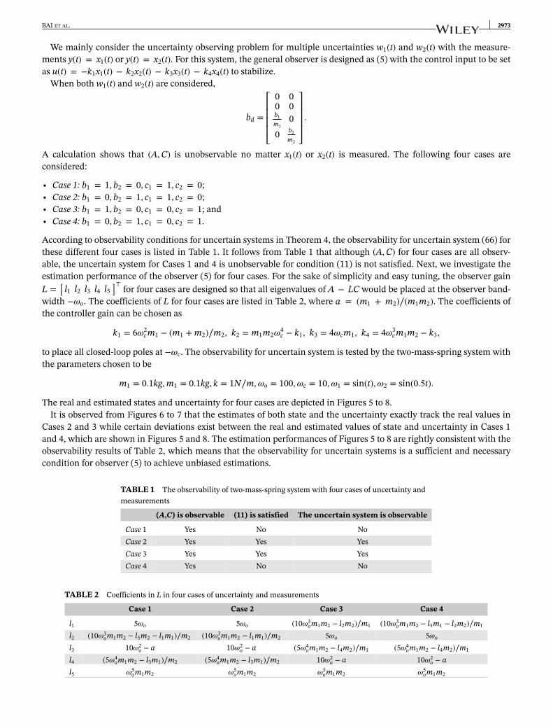
According to observability conditions for uncertain systems in Theorem 4, the observability for uncertain system (66) forthese different four cases is listed in Table 1. It follows from Table 1 that although (A,C) for four cases are all observ-able, the uncertain system for Cases 1 and 4 is unobservable for condition (11) is not satisfied. Next, we investigate theestimation performance of the observer (5) for four cases. For the sake of simplicity and easy tuning, the observer gainL =
[l1 l2 l3 l4 l5
]⊤ for four cases are designed so that all eigenvalues of A − LC would be placed at the observer band-width −𝜔o. The coefficients of L for four cases are listed in Table 2, where a = (m1 + m2)∕(m1m2). The coefficients ofthe controller gain can be chosen as
k1 = 6𝜔2c m1 − (m1 + m2)∕m2, k2 = m1m2𝜔
4c − k1, k3 = 4𝜔cm1, k4 = 4𝜔3
c m1m2 − k3,
to place all closed-loop poles at −𝜔c. The observability for uncertain system is tested by the two-mass-spring system withthe parameters chosen to be
The real and estimated states and uncertainty for four cases are depicted in Figures 5 to 8.It is observed from Figures 6 to 7 that the estimates of both state and the uncertainty exactly track the real values in
Cases 2 and 3 while certain deviations exist between the real and estimated values of state and uncertainty in Cases 1and 4, which are shown in Figures 5 and 8. The estimation performances of Figures 5 to 8 are rightly consistent with theobservability results of Table 2, which means that the observability for uncertain systems is a sufficient and necessarycondition for observer (5) to achieve unbiased estimations.
TABLE 1 The observability of two-mass-spring system with four cases of uncertainty andmeasurements
(A,C) is observable (11) is satisfied The uncertain system is observable
Case 1 Yes No NoCase 2 Yes Yes YesCase 3 Yes Yes YesCase 4 Yes No No
TABLE 2 Coefficients in L in four cases of uncertainty and measurements
Case 1 Case 2 Case 3 Case 4
l1 5𝜔o 5𝜔o (10𝜔3om1m2 − l2m2)∕m1 (10𝜔3
om1m2 − l5m1 − l2m2)∕m1
l2 (10𝜔3om1m2 − l5m2 − l1m1)∕m2 (10𝜔3
om1m2 − l1m1)∕m2 5𝜔o 5𝜔o
l3 10𝜔2o − a 10𝜔2
o − a (5𝜔4om1m2 − l4m2)∕m1 (5𝜔4
om1m2 − l4m2)∕m1
l4 (5𝜔4om1m2 − l3m1)∕m2 (5𝜔4
om1m2 − l3m1)∕m2 10𝜔2o − a 10𝜔2
o − al5 𝜔5
om1m2 𝜔5om1m2 𝜔5
om1m2 𝜔5om1m2
2974 BAI ET AL.
0 5 10 15 20
−505
x 10
time(s)0 5 10 15 20
−101
time(s)
0 5 10 15 20−5
0
5x 10
time(s)0 5 10 15 20
−2
0
2
time(s)
0 5 10 15 20−2
0
2
time(s)
the true valuethe estimate
FIGURE 5 The real and estimated values of states and uncertainty for Case 1 (example three) [Colour figure can be viewed atwileyonlinelibrary.com]
0 5 10 15 20
0
2
time(s)0 5 10 15 20
−4−2
024
time(s)
0 5 10 15 20−4−2
024
time(s)0 5 10 15 20
−4−2
024
time(s)
0 5 10 15 20−2
0
2
time(s)
the true valuethe estimate
FIGURE 6 The real and estimated values of states and uncertainty for Case 2 (example three) [Colour figure can be viewed atwileyonlinelibrary.com]
0 10 20
−5
0
5
x 10
time(s)0 10 20
−0.1
0
0.1
time(s)
0 10 20−1
0
1
time(s)0 10 20
−2
0
2
time(s)
0 10 20−2
0
2
time(s)
the true valuethe estimate
FIGURE 7 The real and estimated values of states and uncertainty for Case 3 (example three) [Colour figure can be viewed atwileyonlinelibrary.com]
FIGURE 8 The real and estimated values of states and uncertainty for Case 4 (example three) [Colour figure can be viewed atwileyonlinelibrary.com]
Moreover, it follows from Table 2 and Figures 5 to 8 that when x1(t) is measured, the uncertain system with w1(t) isobservable, while the uncertain system with w2(t) is unobservable. Conversely, when x2(t) is measured, the uncertainsystem with w2(t) is observable whereas the uncertain system with w1(t) is unobservable. Thus, for given measurement,observability corresponding to different uncertainties may be opposite. Fortunately, the observability criterion (iii) inTheorem 4 clearly tells us the case of uncertainty that can be accurately estimated before we try to design an observerto estimate the uncertainty. This is of great significance both theoretically and practically. On the other hand, for certainuncertainty, different measurements have different observability properties. How to choose the least “feasible” outputto achieve unbiased estimation of uncertain systems is an important problem to be solved. The observability criterion(iii) rightly gives the intuitional answer to this problem. For instance, Table 1 indicates that if we want to estimate w1(t),x2(t) needs to be measured, and similarly, if we want to estimate w2(t), x1(t) needs to be measured, which is verified byFigures 6 to 7.
A comparison of Figures 5 and 8 shows that although the estimations for Cases 1 and 4 are both biased, the deviationfor Case 4 is much smaller than that for Case 1. According to (53) in Theorem 1, the estimation error of unobservablesystem is S−1Δ, which is calculated as the following values for two cases:
The (53) in Theorem 1 quantitatively gives an estimation error of unobservable Cases 1 and 4, which helps to explain whythe deviation for Case 4 is smaller than that of Case 1. Since the estimation value is almost coincident with the true valueof w2(t) for Case 4, the estimate of w2(t) can be treated as “reliable” one, which can be used to approximate the true valueof w2(t) although the uncertain system in Case 4 is unobservable.
6 CONCLUSIONS
This paper analyzes the performance of observer for a large class of uncertain nonlinear systems and proposes a structuralcondition, which is proved to be essential to ensure the convergence of the observer. It is shown that the combination ofthe structural condition and the observability for the augment matrix pair is a necessary and sufficient condition for theobserver to be convergent. By defining observability for uncertain nonlinear systems, it is further proved that the uncer-tain nonlinear systems are observable if and only if both the structural condition and the observability of the augmentmatrix pair are satisfied. In addition, for unobservable uncertain nonlinear systems, which do not satisfy this necessaryand sufficient condition, it presents explicitly a biased estimation error, which can be used to evaluate the estimation
performance of the proposed observer. The numerical simulations for three typical examples are carried out to validatethe theoretical analysis.
ACKNOWLEDGEMENTS
This work was supported by the Natural Science Foundation of China the (grants 61603365, 61873260, and 11801077), theNatural Science Foundation of Guangdong Province (grant 2018A030310357), and the Project of Department of Educationof Guangdong Province (grants 2017KTSCX191 and 2017KZDXM087).
REFERENCES1. Gao ZQ. On the centrality of disturbance rejection in automatic control. ISA Trans. 2014;53:850-857.2. Li J, Qian CJ, Ding SH. Global finite-time stabilisation by output feedback for a class of uncertain nonlinear systems. Int J Control.
2010;83:2241-2252.3. Li SH, Yang J, Chen WH, Chen XS. Disturbance Observer-Based Control: Methods and Applications. Boca Raton, FL: CRC Press; 2014.4. Xie LL, Guo L. How much uncertainty can be dealt with by feedback. IEEE Trans Autom Control. 2000;45:2203-2217.5. Zhang CL, Jia RT, Qian CJ, Li SH. Semi-global stabilization via linear sampled-data output feedback for a class of uncertain nonlinear
systems. Int J Robust Nonlinear Control. 2015;25:2041-2061.6. Chen WH. Disturbance observer based control for nonlinear systems. IEEE/ASME Trans Mechatron. 2004;9:706-710.7. Feng H, Guo BZ. A new active disturbance rejection control to output feedback stabilization for a one-dimensional anti-stable wave
equation with disturbance. IEEE Trans Autom Control. 2017;62:3774-3787.8. Liu JJ, Wang JM. Boundary stabilization of a cascade of ODE-wave systems subject to boundary control matched disturbance. Int J Robust
Nonlinear Control. 2017;27:252-280.9. Guo BZ, Wu ZH. Output tracking for a class of nonlinear systems with mismatched uncertainties by active disturbance rejection control.
Syst Control Lett. 2017;100:21-31.10. Guo BZ, Wu ZH. Active disturbance rejection control approach to output-feedback stabilization of lower triangular nonlinear systems
with stochastic uncertainty. Int J Robust Nonlinear Control. 2017;27:2773-2797.11. Guo BZ, Zhao ZL. Active Disturbance Rejection Control for Nonlinear Systems: An Introduction. Singapore: John Wiley & Sons; 2016.12. Jiang TT, Huang CD, Guo L. Control of uncertain nonlinear systems based on observers and estimators. Automatica. 2015;59:35-47.13. Pu ZQ, Yuan RY, Yi JQ, Tan XM. A class of adaptive extended state observers for nonlinear disturbed systems. IEEE Trans Ind Electron.
2015;62:5858-5869.14. Shao S, Gao ZQ. On the conditions of exponential stability in active disturbance rejection control based on singular perturbation analysis.
Int J Control. 2017;90:2085-2097.15. Xue WC, Huang Y. On performance analysis of ADRC for a class of MIMO lower-triangular nonlinear uncertain system. ISA Trans.
2014;53:955-962.16. Zhou HC. Output-based disturbance rejection control for 1-D anti-stable Schrödinger equation with boundary input matched unknown
disturbance. Int J Robust Nonlinear Control. 2017;27:4686-4705.17. Han JQ. From PID to active disturbance rejection control. IEEE Trans Ind Electron. 2009;56:900-906.18. Zhao ZL, Guo BZ. A nonlinear extended state observer based on fractional power functions. Automatica. 2017;81:286-296.19. Freidovich LB, Khalil HK. Performance recovery of feedback-linearization-based designs. IEEE Trans Autom Control. 2008;53:2324-2334.20. Praly L, Jiang ZP. Linear output feedback with dynamic high gain for nonlinear systems. Syst Control Lett. 2004;53:107-116.21. Basile G, Marro G. On the observability of linear, time-invariant systems with unknown inputs. J Optim Theory Appl. 1969;3:410-415.22. Li SH, Yang J, Chen WH, Chen XS. Generalized extended state observer based control for systems with mismatched uncertainties. IEEE
Trans Ind Electron. 2012;59:4792-4802.23. Söffker D, Yu TJ, Müllter PC. State estimation of dynamical systems with nonlinearities by using proportional-integral observer. Int J Syst
Sci. 1995;26:1571-1582.24. Hammouri H, Tmar Z. Unknown input observer for state affine systems: a necessary and sufficient condition. Automatica.
2010;46:271-278.25. Chang JL. Applying discrete-time proportional integral observers for state and disturbance estimations. IEEE Trans Autom Control.
2006;51:814-818.26. Yan BY, Tian ZH, Shi SJ, Weng ZX. Fault diagnosis for a class of nonlinear systems via ESO. ISA Trans. 2008;47:386-394.
27. Su J, Ma H, Qiu W, Xi Y. Task-independent robotic uncalibrated hand-eye coordination based on the extended state observer. IEEE TransSyst Man Cybern B Cybern. 2004;34:1917-1922.
28. Sun M, Wang Z, Wang Y, Chen Z. On low-velocity compensation of brushless DC servo in the absence of friction model. IEEE Trans IndElectron. 2013;60:3897-3905.
29. Xia Y, Zhu Z, Fu M, Wang S. Attitude tracking of rigid spacecraft with bounded disturbances. IEEE Trans Ind Electron. 2011;58:647-659.30. Xue WC, Bai WY, Yang S, Song K, Huang Y, Xie H. ADRC with adaptive extended state observer and its application to air-fuel ratio control
in gasoline engines. IEEE Trans Ind Electron. 2015;62:5847-5857.31. Kalman RE. Mathematical description of linear dynamical systems. J Soc Ind Appl Math Ser A Control. 1963;1:152-192.32. Kreindler E, Sarachik P. On the concepts of controllability and observability of linear systems. IEEE Trans Autom Control. 1964;9:129-136.33. Gao ZQ. Scaling and bandwidth-parameterization based controller tuning. In: Proceedings of the American Control Conference; 2003;
Minneapolis, MN.34. Zhang H, Zhao S, Gao ZQ. An active disturbance rejection control solution for the two-mass-spring benchmark problem. Paper presented
at: 2016 American Control Conference (ACC); 2016; Boston, MA.
How to cite this article: Bai W, Chen S, Huang Y, Guo B-Z, Wu Z-H. Observers and observability for uncer-tain nonlinear systems: A necessary and sufficient condition. Int J Robust Nonlinear Control. 2019;29:2960–2977.https://doi.org/10.1002/rnc.4531