OCEANOORAPHIC ANALYSIS MANUAL FOR ON-SCENE PREDICTION SYSTEMS. CUl

UNCLASSIFIED N0-RPZ2ON

EIIIIIIIIIIIIuEEEEEEEEEEEEEIKIEEEIIIIIEEEEEEEIIIEEEEEIIIImhhllllllllllilu

1111.25 11111_1.4 II .6

III- '[W ;1,1 III -

PHOTOGRAF I THIS SHEET

,.~EVEL.N v|Oe ,,.; ,. ,v o,Nava cVP t&U&c C, rINVENTORY

____________, ' Sl. .uos, 3

8 DOCUMENT IDENTIFICATION may (776

DISTRIBUTION STATEMENT AApproved for public release;

Distribution Unlimited

DISTRIBUTION STATEMENT

ACCESSION FORNTIS GRA&iDYIC TAB DUNANNOUNCED Q]JUSTIFICATION ELECTE

BY S JUN 2 6 1980 i

BY'

DISRIBUTION, DAVAILABIL[TY CODESDIST AVAIL AND/OR SPECIAL. DATE ACCESSIONED

NVTE: C'"!ssified reerences riarermain as lis~ed.

Per: Mr. Dale Tid-ick,N(10, NSTL, Bay St.

DISTRIBUTION STAMP pL,

DATE RECEIVED IN DTIC

PHOTOGRAPH THIS SHEET AND RETURN TO DTIC-DDA-2FORM 7DOCUMENT PROCESSING SHEET

DTIC OCT 79 70A

- - k

- - -~

I

9- .K,~' v..

rNOO RP-20

$

OCEANOGRAPHIC ANALYSIS MANUAL

FOR ON-SCENE PREDICTION SYSTEMS

ALVAN FISHER, JR.

MAY 1978

Approved for public release, distribution unlimited.

NAVAL OCEANOGRAPHIC OFFICENSTL STATION

BAY ST. LOUIS, MS 39522

I

FOR WORD

The collection of environmental information by men-of-war datesto the earliest days of the United States Navy. In the past, few ofthese data were processed Immediately; most were logged for laterprocessing and analysis at stations ashore. Modern fleet units donot have this luxury, for they must be able to respond rapidly to anynumber of possible threats. Thus, it is Imperative that forcesafloat not only collect environmental data, but process and analysethe data as well. The procedures given in this text providetechniques necessary to convert oceanographic data into a meaningfulanalysis for subsequent conversion into tactical indices throughacoustic performance prediction using systems such as the IntegratedCommand ASW Prediction System (ICAPS).

R McDONNELL~aptan, U.S. Navy

Commander

iiii

ACKNOWLEDGMENTS

The author wishes to note the many suggestions and guidanceprovided by G. L. Hanssen. Of equal importance is the assistancein manuscript preparation given by I. Pelaez, D. L. Waters, andA. G. Voorhets. The task was funded as part of the IntegratedCommand ASW Prediction System (ICAPS) Program under the cognizanceof the U. S. Naval Oceanographic Office.

f

iv

JCONTENTS

Page

I. INTRODUCTION i

II. DATA REQUIREMENTS .......... ..................... 2

III. THERMAL STRUCTURE DATA SOURCES .......... .......... 3

IV. QUALITY CONTROL ........ .. .................... 3

V. OCEANOGRAPHY ......... .................... 6

Water Masses ........ .. .................... 6Oceanic Fronts .......... .................... 6Frontal Acoustics ......... ................... 10

VI. ENVIRONMENTAL DATA ANALYSIS ........ .............. 10

Environmental Data Collection ...... ............. 10Oceanographic Data Processing ............... .I. 11Acoustic Data Processing .. ............. 13Plotting and Analysis .. ............. 16

VII. REFERENCES ...... ...................... .25

FIGURES . . . . . . . . . . . . . . . . . . . . . .

1. Worldwide distribution of oceanic fronts . . . 92. Effect of temperature versus depth in sound speed

computations (metric units) 14

3. Effect of temperature versus depth in sound speedcomputations (engineering units) .... ......... 15

4. Sample oceanographic data summary sheet ...... .175. Rough oceanographic plotting sheet ........ .186. Smooth SST analysis ... ............... . 197. Smooth SLD analysis ... ............... . 208. Smooth water mass analysis .. ............ . 229. Typical water mass sound speed profiles ..... 2310. Typical water mass propagation loss-versus-range plots . 24

TABLES

1. Criteria for rating the relative strength of oceanfronts ..... ..................... 7

* v

0

I.

Page

VIII. APPEN]DIXES

A. Bathythermogram Radio Message Format. ......... 27B. Examples of XBT Malfunctions... ........... 35C. Water Mass Criteria - North Atlantic Ocean/

Mediterranean Sea....................47D. Water Mass Criteria - North Pacific Ocean .. ...... 63E. Water Mass Criteria - Indian Ocean. .......... 81F. Glossary of Acronyms..................93

vi

I. INTRODUCTION

Effective use of assets available to ASW units requires anawareness of the surrounding environment. This is particularly trueof underwater acoustics because of the effect of temperature, salinity,and pressure (depth) on sound velocity. An experienced ASW unit"ommander recognizes that changes in these parameters and the resultingchange in sonar range prediction greatly affects the ability to detectand track potentially hostile submarines. Although oceanographicanalyses are available from shore-based Fleet Weather Facilities duringperiods when electronic emission control is not in effect, they oftendo not have sufficient data input and detail to be satisfactory. Thepurpose of this report is to describe some techniques for on-sceneanalysis of oceanographic data as a necessary step in the preparationof valid and timely acoustical/tactical products.

On-scene analysis of oceanographic data is not new. Experimentalanalyses were made in support of carrier air groups during the late1950's. The availability of improved sensors, faster and more efficientcomputers, and a better understanding of oceanic and acoustic processesrequires that the older techniques be updated. It is expected that thetechniques described in this publication eventually will be assumed byfully automated systems. Even then, an analyst who understands oceanicprocesses will be required to evaluate the output. The success of anyon-scene sonar range prediction system is predicated on the quality andrelevancy of the input data. For example, depth - temperature valuesinput from an expendable bathythermograph (XBT) probe that malfunctionedfor any one of a number of reasons may produce un'eliable sonar predic-tions. Similarly, data input representative of Slope Water north of theGulf Stream would provide misleading predictions if used in the SargassoSea. It is the responsibility of the oceanographic/environmental analystto assure that input data are both accurate and representative of existingconditions. The preparation of a water mass analysis provides a processthat examines not only the accuracy of oceanographic data, but establishes

the geographic limits of observations with similar characteristics aswell. Unfortunately, the analyst frequently has received little trainingin preparing oceanographic analyses. This text provides a method ofoceanographic analysis of relatively small geographic areas--on theorder of 200 nmi or smaller--as an integral part of on-scene sonar rangeprediction, with particular application to automated systems such as theIntegrated Command ASW Prediction System (ICAPS).

Material covered in this report is divided among three generaltopics: (1) collection and quality control of oceanographic data; (2)major oceanographic features, and; (3) analysis of synoptic environmentaldata to provide near real-time information as to location and characteristicsof such features. Because the report is designed as a guide for ICAPSusers, it occasionally refers to computer software included in thatsystem such as the deep water mass history. However, most of the textwill apply to all systems.

]1

H -" __.. . .. . .. .__.. .I.. . .________._. . .._ ... . .' " . .

II. DATA REQUIREMENTS

Fnvironmental information required for sonar range predictionincludes a sound speed profile from sea surface to ocean floor, waveheights, depth and acoustic reflectivity of the bottom, ambient noise,and scattering coefficients. The sound speed profile normally isgenerated by merging a real-time XBT trace with deep historicaltemperature data, selecting a salinity value for each depth-temperaturepair, and converting these data to sound speeds. Most deep historiesprovide a single set of values for a given area. The ICAPS file,however, provides deep histories for each water mass indigenous to thearea under consideration. Description of the ICAPS history and methodof combining real-time data with historical data is too complex toinclude here, but may be found in reference (1)*.

Water depth and acoustic bottom type are required inputs tocompute bottom bounce and convergence zone propagation. The former maybe determined either by fathometer or reference to nautical charts.Bottom type-required to determine the amount of energy reflected fromthe bottom--is input on a 1 to 9 scale for frequencies at or above 1000Hz with a simplified scale below 1000 Hz (2, 3). Bottom loss type andmean water depth for each prediction area for the Northern Hemisphereand the Indian Ocean may be found on the ASW Prediction Area Charts.These data also are stored in the ICAPS history by 30-minute rectangles,thus enabling the user to default to the history if more accuratepositioning is not required.

Ambient noise--the summation of noise caused by waves,precipitation, marine biota, shipping and industrial noises--detractsfrom the ability to detect potential targets. Ship noise and cavita-tion are the major sources of ambient noise at frequencies below 50 Hz,whereas sea state usually is the largest contributor at frequencies inthe 100 to 5000 Hz range. Depending upon the prediction model used,wind speed or wave heighL is used as input for estimates of ambientnoise in the higher frequency range. Direct ambient noise measure-ments are possible using the AX/SSQ-57 sonobuoy and certain sonars inthe passive mode, but are of limited value because of the rapid varia-tion of ambient noise with respect to time and space and the inadequaciesof recording equipment. Tables are available to compute ambient noiseas a function of region and wave height (4, 5).

To obtain sonar predictions in the active mode, the analystmust determine the appropriate scattering coefficients. Volumescattering--a measure of the amount of energy reflected by suspendedparticles in the ocean, fish, and marine organisms--is directly relatedto the number, type, and distribution of the scatters. Layer scatteringis attenuation caused by the millions of marine organisms which form thedeep scattering layer. Both scattering coefficients are frequencydependent and vary rapidly with space and time. Because real-timescattering data are seldom available, default values are given in ref-erence (6) based upon values developed at the Fleet Numerical WeatherCentral (FLENUMWEACEN).

*References will henceforth be indicated by reference number enclosedin parentheses.

6r2

III. THERMAL STRUCTURE DATA SOURCES

Because sound speed profiles are rarely available to operatingFleet units, real-time thermal structure observations are normally usedin ccnjunction with deep historical temperature and salinity data toapproximate the sound field. Sources of temperature data include theshipboard expendable bathythermograph (XBT)*, thermistors mounted onhelicopter sonars or submarine sail, airborne expendable bathythermo-graph (AN/SSQ-36), submarine bathythermograph, mechanical bathythermograph,injection intake thermometer, and infrared imagery from aircraft andsatellites. Although few ASW units are able to obtain data reportsfrom all of the above sources, most are available from accompanyingunits.

As in all instrumentation, the above temperature sensingdevices are subject to measurement error. The XBT is the most accuratesensor available to fleet units. It has temperature errors within0.20 C 95 percent of the time and depth errors of 2 percent or 5 m,whichever is greater (7). The SSQ-36 is rapidly approaching thecapabilities of the shipboard system, but requires a better readoutcapability. Because submarine-mounted XBT systems are being introducedto fleet units, a data base to compute error rate and accuracy is notyet available.

Few mechanical bathythermograph observations are made today

because of the superiority of the XBT systems. Mechanical BT's aredifficult to keep calibrated, are limited to 270-m depths, and requirethe user to reduce speed to below 15 knots. Injection temperaturereadings are affected by engine room temperature, frequently read bydisinterested engineering personnel, and--because the sensor is locatedat varying depths below the surface--may not truly represent surfacetemperature because of the effect of seasonal thermoclines.

Airborne and satellite infrared (IR) imagery requirecorrections prior to use as sources of surface temperature values.

While correction tables are available for the former, none exist forsatellite data. In the absence of cloud cover and sea spray they providesuperb definition of major oceanic features such as fronts and eddies.Although these data generally are available only to select units; oceanicanalyses made using IR data are broadcast to fleet units by facsimile.

IV. QUALITY CONTROL

All data input to sonar range prediction models or oceanicanalyses must be quality controlled to eliminate misleading data.For example, a study of 411 XBT traces encoded during two fleet exercisesfor transmission to FLENUMWEACEN showed an error rate greater than 60percent (8). After elimination of encoding errors, the errors fellinto three basic types: (1) failure to select depth-temperature pairs

*3athythermogram data from all sources will be referred to as XBT data

because of the predominance of expendable systems.

3

that were representative of the XBT trace, (2) failure to recognizemalfunctioning XBT probes, and (3) positioning errors. If these datawere included in an oceanographic/acoustic analysis they could show

non-existent oceanic features.

With few exceptions, the process of preparing XBT traces forinput into a so'ar range prediction model is like that used to encodethe XBT trace fo.° transmission as BATHY messages. For this reasoninstructions for encoding XBT traces are given in Appendix A. Thepurpose of encoding is to convert a continuous record from an XBT traceto a number of depth-temperature pairs suitable for input to thecomputer*. Computer space may limit the number of data points thatcan be input, e.g., a maximum of 15 points can be used in ICAPS.Although ICAPS input may be in either engineering (OF, ft.) or metric

units (°C, m), current instructions (9) require that XBT messages for-warded to FLENUIMWEACEN be in metric units, thus requiring conversionto metric units during encoding. There appears to be a tendency amongobservers to record temperature values at constant depths (e.g.,100-m intervals) to reduce the number of values that must be converted.This causes some acoustically important features, such as sound channels,to be missed.

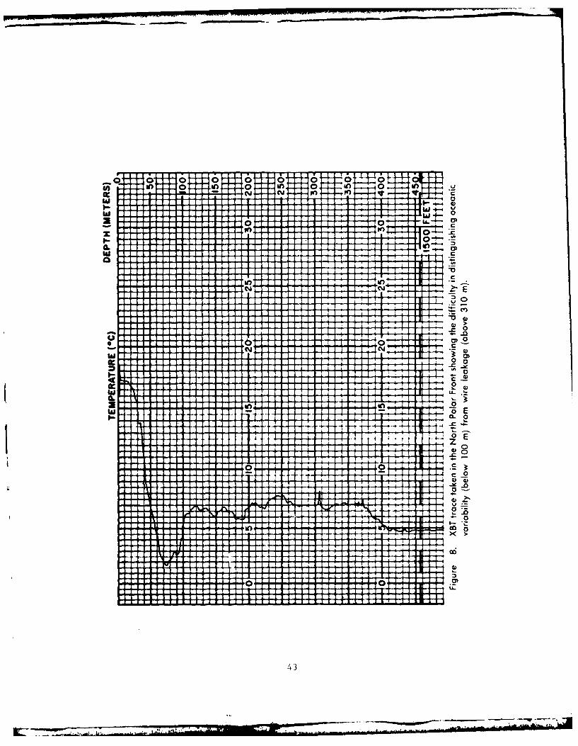
Failure to recognize malfunctioning probes is the most difficultto correct of all error sources. XBT probes frequently are not stowedin upright positions and are left in areas where ambient temperaturesare greater than 320 C (900 F). Under these conditions, the insulationin the probe cannister melts, causing wire leakage, wire breakage, and

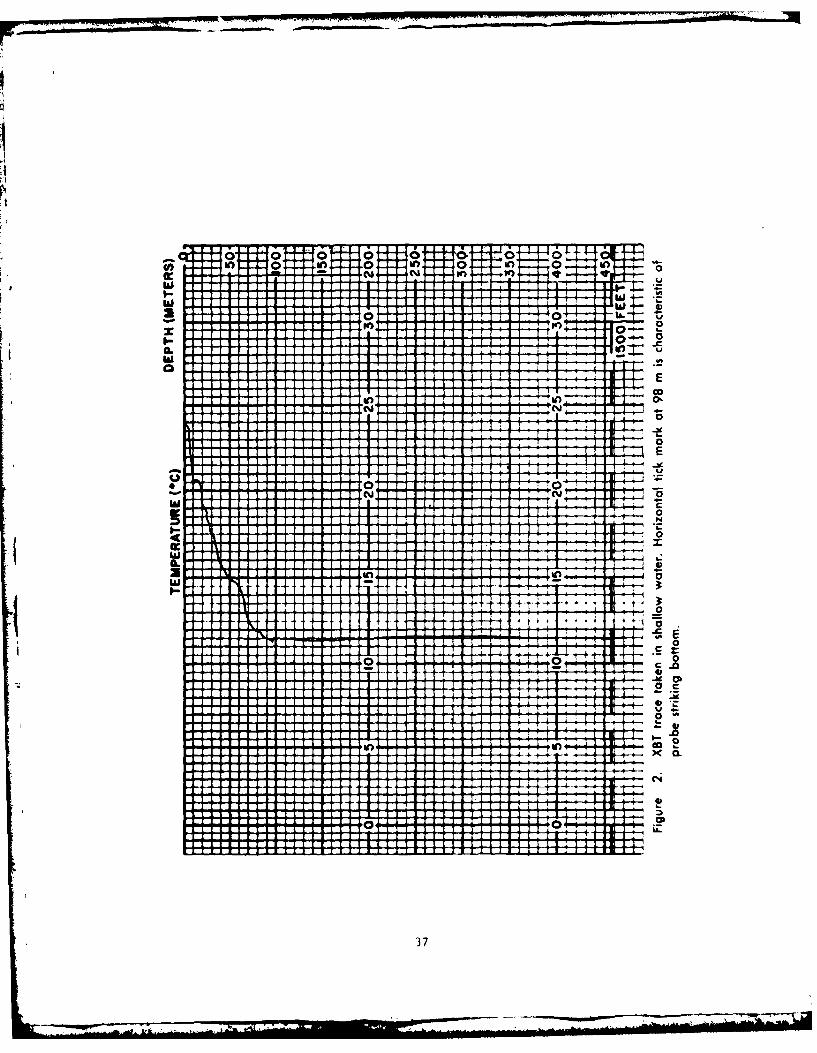
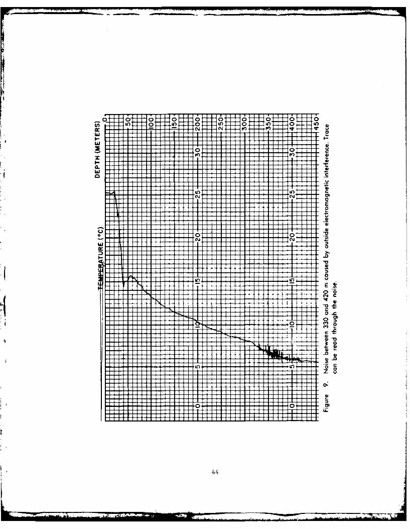
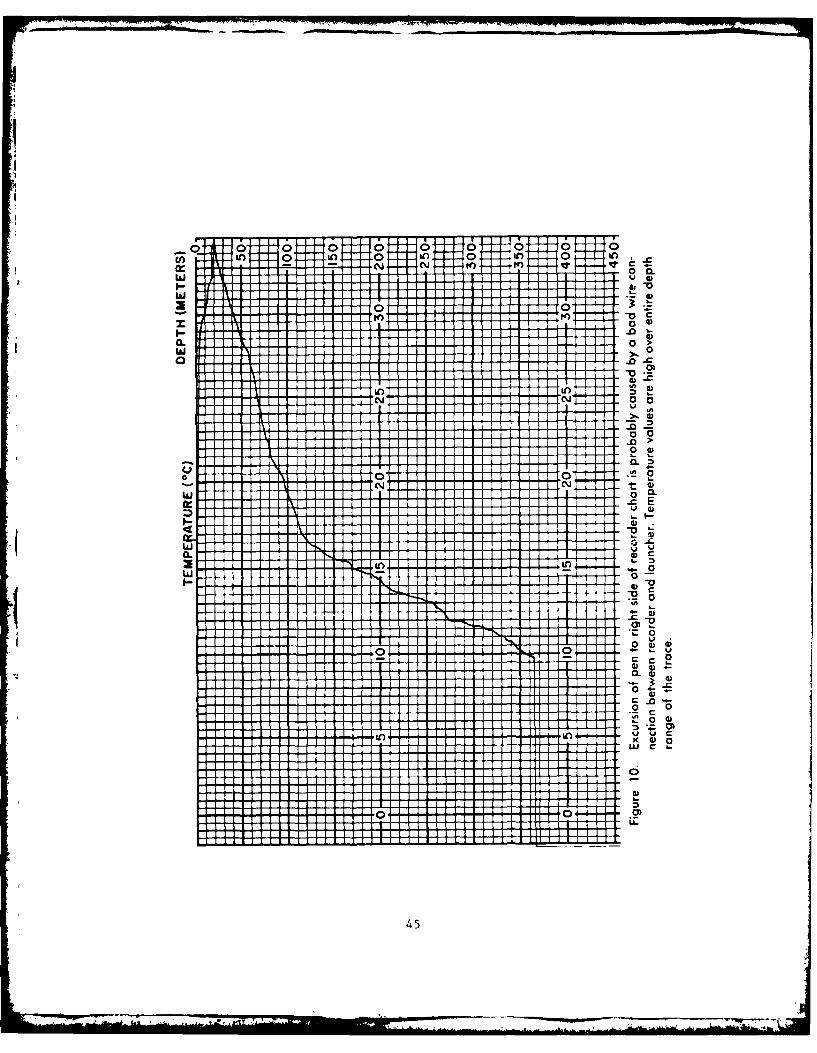
uneven unspooling. Contact with the ship's hull or towed sensor,electromagnetic interference from radar and radio transmission,stretching of the wire near the bottom of the trace, and recorderproblems also cause erroneous traces. In water shallower than 460 m,the XBT recorder continues to function after the probe strikes bott3m.An untrained observer may record this data which, of course, is unreal.Excessive motion of the XBT platform during severe weather, turbulencenear water mass boundaries and, in the case of air dropped probes,washover cause malfunctions from natural sources. Examples of commonXBT malfunctions are provided in Appendix B to help in recognizingerroneous traces.

Position errors may cause apparent radical departures fromactual conditions. For example, an XBT taken north of the Gulf Streamwith an erroneous position could cause the analyst to draw a cold eddysouth of the Stream. The most common sources of positioning errorare transposition of numbers (i.e., 570W instead of 750 W) or erroneouspositions. These errors frequently may be corrected by comparison toa dead reckoning (DR) plot of the reporting unit.

*Future on-scene XBT recorders will likely have digitizers to put the

data directly into the computer, in which case the operator mustedit the trace on a computer display terminal or similar deviceto eliminate errors caused by the XBT system.

4

If data are received in BATHY message format, the analystshould plot the trace to assure correctness. The ICAPS program has anediting feature that automatically plots the XBT's input, relievingthe analyst of this function. In addition to reviewing position,the analyst must check the encoded depth-temperature pairs forfeasibility. Communication garbles, reversed digits, conversion errors,and omission of the 999XX depth indicator can have considerable effect

on the data. Depth and temperature errors caused by transposition ofnumbers (72155 instead of 27155) often can be detected by examiningthe data immediately above and below the point in question. The bestmeans of detecting erroneous data is by comparison with data that isbelieved to be correct. These latter data include observations takenin the same area and the seasonal deep history stored in the ICAPShistory file. An ICAPS file providing XBT traces typical of each watermass by month is being compiled to provide additional guidance.

Wh: a layer of cold, low salinity water (called a temperature

inversion) is found between layers of warmer, more saline water, sonic

energy is trapped within the layer forming a sound channel. Welldefined sound channels may persist for several months near the boundaryof water masses having different temperature-salinity characteristics.Temperature inversions in moderate latitudes rarely occur at depthsgreater than 100 m, whereas weak inversions (0.10 to 0.20 C) are foundto 400 m or deeper in polar regions. An exception to this rule occursin the boundary zone between the Kuroshio and Oyashio Currents in the

western North Pacific where well-defined inversions occur at depthsexceeding 400 m. The analyst should suspect observations that exhibitinversions that are inconsistent with those described above. As a ruleof thumb, deep inversions should be ignored, unless the feature isobserved repeatedly.

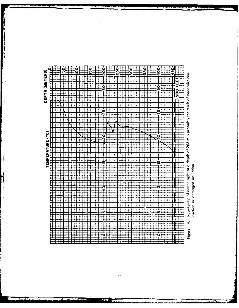
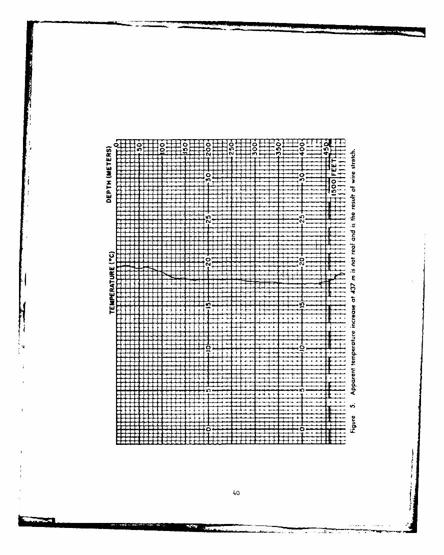
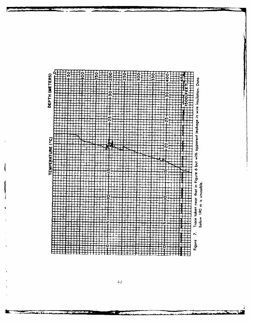
Temperature spikes to the high-temperature side of the trace are*caused by leakage in the probe wire and electromagnetic interference.A gridual temperature increase near the bottom of the trace is a resultof wire stretch or fictitious data recorded after the probe hits bottom.A sudden temperature increase to the right side of the trace followedby constant or slightly decreasing temperature indicates probe failure.These failures are more obvious than those described in the preceding

paragraph and the experienced analyst will have no problem recognizingthem.

When minor discrepancies are noted on an-XBT trace, the analystfrequently tends to correct data by applying a correction to ensuingdepth-temperature pairs. This procedure is not valid and should be

used only as a last resort. If data are plentiful, the analyst shoulddisregard an observation that differs markedly from surrounding observa-tions. In the absence of considerable data the analyst cannot eliminatean observation if it is possible that it indicates the presence ofmesoscale* oceanic feature such as an eddy.

*On the order of 100 kilometers in size.

5

V. OCEANOGRAPHY

Water Masses

The near-surface layer of the ocean is not homogeneous, butis divided into numerous water masses, each having a unique temperature-salinity relationship. Thus, water north of the Gulf Stream is readilydifferentiated from water to the south of the Stream by its relativelylow temperature and salinity. At depths of 200 to 300 m--whereseasonal change is minimal, but within the depth range of the XBT--water masses can generally be identified from thermal characteristicsalone (1). For example, during June 95 percent of sea surface tempera-tures (SST) in slope water fall in a range of 16.30 to 26.60C; differinglittle from the range of 21.40 to 27.6 0 C found in the Sargasso Sea.However, at a depth of 200 m the ranges differ considerably: 9.40 to14.5 0 C in slope water in contrast to 16.50 to 20.0°C in Sargasso water.

Where temperature values at 200 m are similar for adjacentwater masses, a second criterion is required to separate them. Forexample, both Gulf Stream water and Sargasso water have a temperaturerange of 150 to 250 C at 200 m; however, a layer of near-isothermal waterextends to depths exceeding 300 m in the Sargasso Sea, but not in theGulf Stream. Examination of oceanographic data from the northwestern

Sargasso Sea showed that 95% of all observations in that area had atemperature difference between -1.60 C and O.O°C in the layer between200 and 300 m. Thus, the temperature difference between 200 and 300 mis used to distinguish Sargasso water from Gulf Stream water. Additionalinvestigation indicated that the temperature difference criterion workedequally well in other areas, and it has 6een adopted as a 'tie breaker'when temperature criteria are similar at the 200-m level. It should benoted that some water masses occur in the near-surface layer only anddo not extend to 200 m. Because these changes occur within the depthrange of XBT, a single historical file is sufficient for both watermasses.

Oceanic Fronts

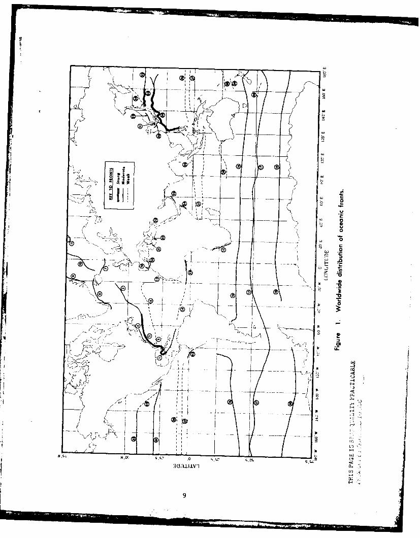
Considerable changes occur in the temperature-salinitystructure in both the horizontal and vertical planes in the boundaryzones between water masses. These zones--called oceanic fronts--areareas of intense mixing, generally 10 to 50 nmi in width. Surfacetemperature differences across a strong front, such as the Gulf Stream,may be greater than 100 C with horizontal gradients approaching 20C/nmi.It is not unusual for multiple gradients to occur in step-like progres-sions across a front. Salinity difference across a strong front mayapproach 2 parts per thousand. The different temperature and salinityregimes found on either side of the front cause density gradients acrossthe front so that the lighter water mass forms a wedge above theheavier (denser) water mass. Thus, the front at depth may be offsetconsiderably from the surface expression of the front. Figure 1 showsthe worldwide distribution of fronts based on the criteria providedin table 1 (9).

6

Anomalous features such as upwelling and eddies may occurwithin a water mass. For example, strong winds accompanying a weathersystem can cause divergence of surface water, allowing upwelling of

cold sub-surface water. Convergence of surface water may cause poorlydefined fronts such as those found in the Sargesso Sea. Instability ofdynamic features cause wave-like meanders to form and subsequentlyprogress as waves along a front. Warm eddies of Gulf Stream origin

may be injected into slope water northwest ci the Stream when meandersbecome unstable. Similarly, extreme meandering of the Gulf Streaimsimilar to the ox bow pattern of old rivers may entrap slope water,thus causing cold eddies in the Sargasso Sea. Eddies range from 50 to

200 nm in diameter and can be expected to retain the circulationpattern of their origin. Eddy life span varies from weeks in the caseof a warm eddy to as long as two years for a cold eddy. Although

eddies and meanders have most frequently been described along majorfrontal systems such as the Gulf Stream and the Kuroshio, weakeranomalies no doubt occur near weaker fronts.

Longevity and intensity of fronts and eddies are greatlyaffected both by existing conditions of contiguous water masses and theoverlying atmosphere. Cold eddies, being denser than the surroundingwarm water, will sink at a rate of up to 1 m per day. Thus, an old,cold eddy may not be evident from surface observations alone. Surfacewarming of fronts during summer frequently masks the surface indicationsof a front; however, subsurface horizontal temperature gradients andsound channels may exist throughout the summer. Warm eddies lose heatto the atmosphere faster than the surrounding cold water in winter with

the result that surface cooling may mask the eddy. Masking also occursin summer when the surface of the surrounding cold water may be warmedto near that of the eddy.

TABLE I

Criteria* for rating the relative

strength of ocean fronts

Maximum change Change in

in sound speed Sonic Layer Depth Depth Occurrence

(m/sec) (m) (M)

Strong 30 150 1000 year-round

Moderate 15-30 30-150 100-1000 year-round

Weak 15 30 100 selectedseasons only

*Table taken from reference (10)

7

.4 J 4 J ~5.44

4J 4J V"..4d U0 5.C4

~N54 .4"4.4& 4C: -4o0 9v V oE $4 4 > . 0 r.

.H-4E I r4 ) CJ ) 1 0-4 -4 O". CI) 4J > .W

Sn 4, 8 4.) ' r

41 to 0Odd 1 1

CL4 C:5. N w H H 44 4" f

0. r o o1410 p.HW3 E )z(

( C14 N N C

5.44

r-4 0-

p. 0

0H 41)po5 4.J rU) 54 r. 0 0 4

"-4 0 0 415.4 -

0 w (1)4. N -HJ 04P '4~ 04 r- 0'A

'U 8 $5J O4 H SNJ44 C-: C1

44 ~ ~ ~ 0 4J~ w - i 4kwr4 ) 0 -H 4 a 4)'r4) to 41)

$ N4 ~ .4 154"-4 " - .g .

-. A 9 8 --4 'or, 2W'0'44C 000 - 4) 8 .U)wCk -W $N4 4.I-W 0 Id 0~ IM45 t,4~4 8 4 -8

W W4J p.)4 1 4 U 4 -1 -4 4 O n w c

04 Nq 0 00

1-4 w 4-4 4-(d4-4 . ,4 r4C'

0 4 U 4 W

u Zrn n e H 0 go(n8~$4

ail,

KC

vIk

2Y'0

_ -

'-- 0

~e

Frontal Acoustics*

An oceanographic front is not only a boundary separatingtemperature-salinity regimes, but also separates acoustic regimes.

Because dynamic instability is inherent to frontal regions, acoustic

conditions can be expected to vary considerably. Variations that

occur during a frontal transit include:

e Surface sound speed may differ as much as 30 m/s oneither side of the front.

9 Differences in sonic layer depth of 300 m can exist oneither side of the front depending upon season.

0 Changes in in-layer and below-layer gradients usuallyaccompany changes in surface sound speed and sonic layer depth.

e The depth of the deep sound channel axis may differ byas much as 800 m on either side of the front.

e Increased biological activity generally found along afront will increase ambient noise and scattering.

* Sea-air interaction in a frontal zone can cause a

dramatic change in sea state when wind opposes ocean currents, thus

increasing ambient noise.

e Refraction of sound rays passing through a front atoblique angles may cause bearing errors.

e Interaction ot the water masses on either side of the

front may cause near-surface sound channels (temperature inversions).

VI. ENVIRONMENTAL DATA ANALYSIS

Environmental Data Collection**

Adequate XBT data coverage in operating areas is needed to

delineate water masses, ocean fronts, eddies, and other thermalfeatures that affect sound propagation. However, the limited availability

of computer processing time will, in most cases, preclude converting

all XBT data collected into sonar range predictions. Even if it werepossible to process all XBT data collected, it would be difficult toeffectively present all the computed information to users owing to thesheer number of the graphics generated. Therefore, it is importantto carefully analyze the ocean environment to determine areas of common

thermal structure, ocean fronts, and eddies. Once analyzed, XBT datarepresentative of each water type present can be processed, and products

from these data keyed to a water mass boundary chart can be presented to

*The material in this section is based on a report by Cheney and Winfrey (10).**Material in this section is based on reference (6).

10

the user. Processing time may be reduced considerably by use of theICAPS editing feature. Presently, XBT data must be manually plottedand analyzed to determine which profiles should be submitted foracoustic processing. The Analysis Section is intended to provideguidance in plotting and interpretation of environmental data.

An oceanographic analyst must coordinate the preparationof on-scene XBT data for the computer operator and establish therequirements for specific ICAPS program runs. XBT drops, reportedfrom naval, research, and commercial vessels on a regular basis inthe form of BATHY reports (9), provide the best source of oceanographicdata. When several escorts are in company, observations usually aretaken by assigned BT guardship duty. In addition, AXBT observationsmay be available from carrier and land-based air groups. Arrange-ments should be made to assure that information copies of all XBTdata are channeled to the oceanographic analyst, since the presentOPNAV instructions specify that XBT data can be transmitted directlyby at-sea observing units to FLENUMWEACEN (9). Because of the many

* errors made in encoding BATHY messages the analyst should use theoriginal XBT trace to prepare the analysis, whenever possible.

If the complexity of the ocean environment requires morefrequent XBT drops from surface units to adequately delineate watermasses in a given operating area, the usual BT guardship concept canbe amended to furnish additional data, particularly if the escorts are

in close formation. By this amended procedure, drops are made at

staggered times so that fewer ships report to the flagship at any onetime. For example, destroyer A would make a drop at 0200Z, destroyerB at 0400Z, and continue with subsequent drops at 4-hour intervals

thereafter. Such a schedule permits a steady flow of data to theanalysis team, eliminates a heavy communication load at the normalreporting time, and permits better sampling of the ocean by a more

even distribution of drops. Many destroyers make routine hourly dropswhen engaged in ASW operations, and these data may be of great valueto the environmental teams. It also may be possible to obtain addi-tional data in remote areas by vectoring patrol aircraft to thoselocations. Observations taken in this manner in future operatingareas are particularly useful.

Oceanographic Data Processing

Detailed analysis of XBT's to delineate water mass and otherthermal features is a complex procedure and entails the predetermina-tion of water mass characteristics and careful matching of observedXBT's to those criteria in order to classify them. The ICAPS programincludes routines to automatically classify XBT data by water mass

as an aid to on-board analysis. Units without ICAPS can manuallyanalyze the data using Appendixes C through E to determine water mass

criteria. Oceanographic data normally plotted include sea surfacetemperature (SST), sonic layer depth (SLD), and water mass boundaries.

ii

The analyst may wish to plot temperature at the 200-m level (T200)*

and the temperature difference between 200 and 300 m (DT) as an aidin water mass identification, temperatures at selected depths, andtemperature gradients (in-layer, below-layer).

The initial step in preparing an analysis is the collectionand examination of available data. Obviously, erroneous data shouldbe discarded and questionable data identified. The analyst isencouraged to enter the data in a log such as that shown later inthe text, both as an aid in preparation of the analysis and as arecord for later reference. It should be noted that all units aregiven in the metric system in order to be consistent with the currentBATHY message format (9). SST is generally available from XBT observa-tions and injection intake thermometer reports. The latter data areparticularly subject to errors and must be used with care. Temperature

values at specified depths (200 and 300 m in the sample given) and,where desired, additional information are computed.

The temperature difference between 200 and 300 m is computedusing the relationship

DT = T300 - T200

Some analysts like to determine the temperature gradientsimmediately above and below sonic layer depth to provide a crude

measure of refraction of sonic energy. The in-layer temperaturegradient giving temperature gradient per hundred meters between thesurface and SLD is determined from the relationship

ILG = (TSLD - SST) x l0/SLD

The below-layer gradient is normally defined

BLG = (TL - TSLD) x bO/L

where L is the thickness of the layer considered below SLD (normal 25or 30 m) and TL is the temperature at the bottom of that layer.

In each of the above equations the values are adjusted toreflect the gradient per 100 m, thus permitting comparison among ob-servations. Values that differ considerably from neighboring valuesShould be treated with suspicion. Particular variability in thermal

structure data can be expected near oceanic fronts. Although XBTtraces normally have an isothermal or slightly negative ILG, positivegradients are not unusual in frontal, coastal, and polar regions. Anincrease of temperature greater than 0.10 C at depths below 200 m

should be questioned.

*Hereafter, temperature levels will be indicated by the letter "T"

followed by the depth (e.g., T200, TSLD).

12

Acoustic Data Processing

Acoustic data normally plotted include SLD, areas whereconvergence zone (CZ) mode of sonar ranging is possible, and extentand axial depth of near-surface sound channels. Because sound speeddata are rarely available to Fleet ASW units, sonic structure isnormally estimated from thermal structure data. Therefore, the previouscomments on processing of oceanographic data apply equally well tothis section.

Sound speed is affected by depth and salinity as well astemperature. Although salinity has relatively little effect, depth(pressure) may have considerable effect on the determination of SLD.Where slightly negative temperature exists, the effect of depth may

be sufficient to cause the sound maximum to occur at the bottom of thelayer. For example, suppose that a near-isothermal layer occurredwith a surface temperature of 15.10 and a temperature of 14.90C at a

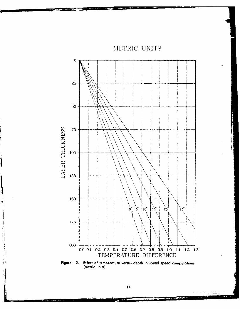
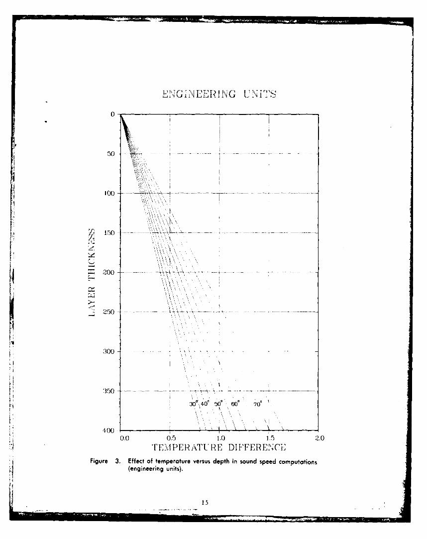
depth of 50 m. The 0.20 C temperature decrease in the layer causes adecrease in sound speed of 0.6 m/s. However, the effect of the 50-mdepth increase causes an increase in sound speed of 0.8 m/s for anet increase of 0.2 m/s. Figures 2 and 3 give the thermal change thatcan exist at various temperatures without overcoming the effect ofdepth. In the case of the previous example, enter figure 2 at a depthof 50 m and move horizontally to the nearest temperature line (150 C).

Then move vertically down to the temperature scale where a value of0.260 is read. Any temperature change less than this (0.20 in theexample) is insufficient to override the effect of depth. SLD willthus be at the bottom of the slightly negative temperature layer.

If the layer thickness is greater than the maximum depth shown on thegraphic (e.g., 260 m), simply solve the problem by using two layers(200 m + 60 m) and add the results.

A similar effect occurs in areas such as the Sargasso andMediterranean Seas and in the Arctic, where a seasonal thermoclinedevelops above a near-isothermal layer during spring and summer. Asound minimum occurs at the bottom of the seasonal thermocline and

the effect of depth overrides the slightly negative temperature gradientforming a so-called 'depressed' sound channel. Figures 2 and 3 againcan be used to determine if the near-isothermal layer forms a depressedsound channel. The channel axis will normally be at the top of thelayer.

When sound speed near the ocean floor is greater than thatat the surface, some of the sonic energy originally refracted downwardtoward the bottom will be refracted upward toward the surface, forminga convergence zone. Range, width and intensity of the CZ is a functionof depth excess; that is, the vertical distance between critical depth*and the bottom. Depth excess generally must be at least 1000 m if CZ

propagation is to be operationally useful. Range to the inner edge of

*Critical depth is that depth below the deep sound channel axis where

sound speed is equal to that at SLD.

13

METRIC UNITS

50-.---- _

S100-i-----

_j 125- _- - 1

150-

0' 5 V? 15' 200 25'

200- .

0.0 0.1 0.2 030.4 0.5 0.6 0.7 0.8 0.9 1.0 1.1 1.2 1.3TEMPERATURE DIFFERENCE

Figure 2. Effect of temperature versus depth in sound speed computations(metric units).

14

ENl~GiNEEF?1NG UNITS

50 ___

2 0 0 ------- --- - - - - - _ _ _ _ _ _ _ _

VV

250 ,

300 ----

350--

V ~30 \40 50 66' 0

400 '

0.0 0.5 1.0 1.5 2.0

~1TEMIPERATURE DIFFERENCE;(Figure 3. Effect of temperature versus depth in sound speed computations

(engineering units).

p 1 5

the first CZ annulus varies between 33 and 70 kyds, depending upongeographic area. Areas of high insonification at ranges less than33 kyds, or where depth excess is insufficient for CZ propagation,are probably the result of bottom bounce (BB) propagation.

Plotting and Analysis

The experienced analyst develops techniques over the yearsthat permit rapid plotting and analysis of environmental data. Thefollowing suggestions are provided as an aid in developing thesetechniques. In the example given only a portion of available data isused. The decision as to what data should be plotted depends upon whatinformation is required for subsequent briefings. For example, deter-mination and plotting of the temperature difference between 200 and 300

m (DT) is meaningless if it is not required for water mass identification.

Choice of plotting base and method of plotting are theprerogative of the analyst. Where a mercator base is desired, nauticalcharts or plotting sheets are recommended, but graph paper ormaneuvering boards also may be used.

Use of a summary sheet may be helpful in preparing thedata for plotting. A sample summary sheet is shown as figure 4 withfictitious BATHY and SST data. Data entered on this sheet will be usedlater to prepare a sample analysis. Ship name, DTG, position, thermalstructure data at various levels, SLD, and water mass are generallysufficient. Water mass is determined from Appendix C (North AtlanticOcean), using T200 and DT. Any observations not meeting the qualitycontrol criteria discussed earlier or falling outside water masscriteria given in Appendixes C through E should be used with caution.ICAPS can store XBT profiles during the data processing routine andthe analyst can rapidly recall this file. If an XBT probe mal-functioned below the surface layer, SST and SLD may be used if inagreement with surrounding observations.

After this summary sheet has been completed and a preliminaryerror check made, the data should be transferred to the plotting sheet.

Figure 5 shows a plotting sheet with position, DTG, and applicabledata entered from the summary sheet. Symbols or colored pencils maybe used to identify each ship--again this is the analyst's choice.Position errors are frequently revealed by computing the speed of

advance (SOA) between successive observations. For example, an SOAOf over 56 kts. is required to achieve the 07/0000 position of the

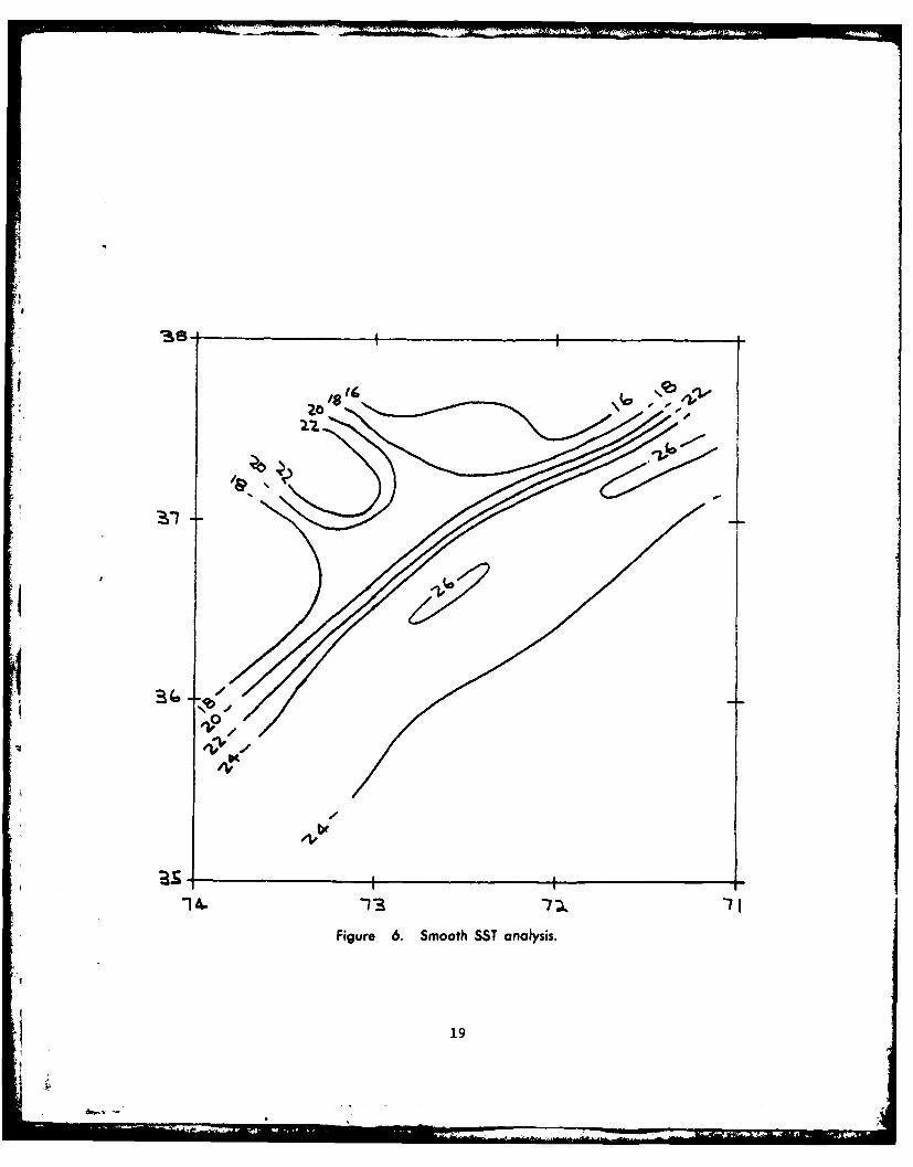
MCCANDLESS as recorded on the sample plot. Therefore, this observationshould be discarded if the correct position cannot be determined fromother sources (DRT plot, Quartermaster's log, etc). Pertinent informa-tion--such as SST, SLD, and water mass--may be plotted either on thebase chart or on overlays of tracing paper (figures 6 and 7). It ishelpful to analyze SST first because these data are more plentiful,thus permitting definition of the more obvious ocean features. Sub-sequent analyses--such as the SLD analysis shown--normally are configured

to agree with the SST analysis.

16

, , IP b'-Wr L 7 L0- S .T &7 is," -ram o r.o -. I-

. 5 -o 7- -71-3 €, S T It 8 .- . A Gl.1-31 1- t - .. ta.V I . -l.4 SL

Qp.00 21-42. 14-sq tsl LL I % 0-0 -0S%1 1-- So 73-41 ( i. I 4 ?.-A -1-l1 %._

CO ' b -a0 -13 -.. 171.o 1 1 I .. . , - . .3 .T .IS1€.o -14-2L4 "1-O'S ZL4.'I o \ .Vj .0! -6-1 G-5I6o "i ,'5-11 14 -4S. %... 12 IS5 14. 6 -a.-? '-1"10 B(- 7"--4. a6.3., to IO. 1E: I .1 -C-2 S P%goo '&of -I -£ .5. IS 11.1 12.0 -0.S S A

IAoo- 30 -. l1 -34- 2.3. i. IA, II l . -

! 2.00 "U 4 -1-I-SI I".3 7 I's . 7- .o - - SA"7/oo -J7-£. - , j_ ,0 ~ a4 1 o a .A S34 _j?

=0 3100 14 it-at 13 a 11.1 -4,2 -0.4- L..M O,'. ]1aoo -1- 7 -'1 3. 3a. it.ib 5. - 1 L

-0 7 -1S I 1 Q 1*.5 -t. - __

icrhyb (Daoo 'i -o .iL3. ..- L 3.O i t .' I 't -7 -21.o1,

____ .30.0 31,-Si 7 -o. ..i i2- . I. - oi. 3

i ,000 €-4; I -0 S I .6 - .,_ _0_ 34- t -a a4 to . -2

Fu 4 Sample a su m r s t.____ 0 0 ~ 3 .. 10. 12-41 I1.6 .. jI

cl__ og. ssa 74-0 S :A Il l - t- -' 1 S

010_ p -o MS4 -a -4 i. R A.1 1-3.1 -1.4.J S

_ _ _ _ 0400 'Sb4jS -1A-0 231 11. 1- IncG -0.- SA______U 345 11.-A 30 12 ___ 1 _s __a-ro

a co 440'1-40 'S- a 11 I. -1-4- S_ _47c 1 -14- ___ 11_S1 11_i __

7Z;oo 36-So -1.1 R A. o__ I_ Q4__

ir 31-00 11-S4 .S ___ _ _ __ __ __

Figure 4. Sample oceanographic data summary shoot.

1 7 ,

:i I 0 v.00o ~ 0.+0cu o °

II

%6, .,

% 6.0 )( S

ai a*

SL .Sa-

"8 a

OL %4vj. Q

woo I,

S1m-

~s. .

-1 4 1 2.

Figure 5. Rough oceanographic plotting sheet.

18

07k

Ar

Figure 6. Smooth SST analysis.

19

~~0

'74. I's

Figure 7. Smooth SID analysis.

20

During the plotting and analysis phases the analyst mustapply his knowledge of oceanography with respect to (1) eliminationof data that vary markedly from other data and (2) the properties ofmesoscale oceanic features of the area. For example, the 7/0100 XBTdrop made by the BROWN showed an SST of 29.5 0 C; some 60 C higher thanother data in the same general area. Although SLD, T200, and T300 werereasonable, uncertainty as to the accuracy of the observation prohibitsits use in the analysis. However, the 6/1800 and 6/1900 data collectedby the MCCANDLESS to the southwest of the aforementioned BROWN observa-tion show characteristics of Gulf Stream water. The presence of coldwater adjacent to the MCCANDLESS observations indicates that the warmwater is isolated from the Gulf Stream as an eddy.

Knowledge of oceanic processes is helpful in maintainingobjectivity. In frontal zones, where water masses of differenttemperature-salinity characteristics occur, it is common for thewarmer, more saline (and thus lighter) water to override the colder,less saline water with the result that SLD may approach the surface.In the example given, a zone of near-zero SLD is likely near theoceanic front separating slope water and Gulf Stream water.

The completed water mass analysis (figure 8) can now bedrawn. Prior to labeling the analysis, XBT traces representative ofeach water mass should be selected. In selecting a typical trace theanalyst should especially consider shape of the trace, T200, SLD, andSST. Once a trace has been selected, its position should be plottedon the analysis along with identification (A through D in the analysis).Name of water mass and variability of SST and SLD now can be added tothe water mass on the analysis.

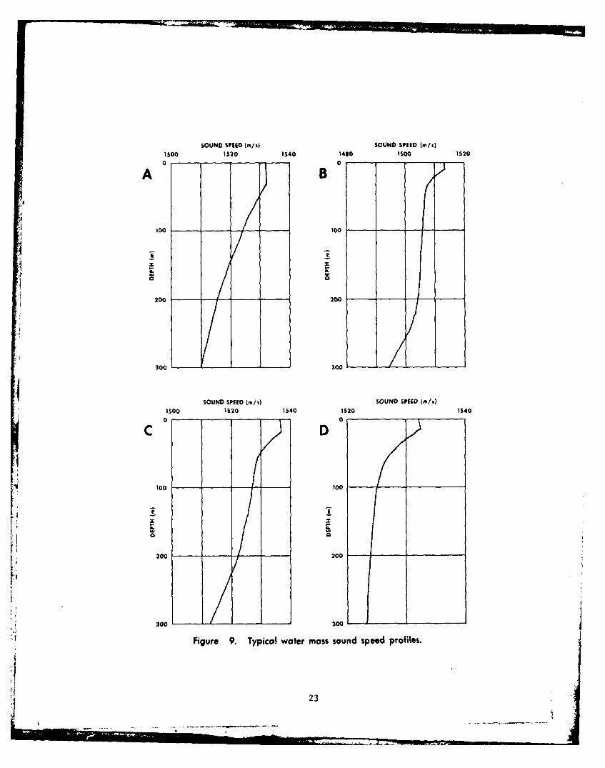
The full suite of ICAPS acoustical and tactical products cannow be made using the respresentative XBT traces selected for eachfrequency and source depth/hydrophone depth desired. Other environ-mental data (wave height, bottom classification, water depth, ambientnoise, scattering coefficients) will be required to compute passiveand active sonar ranges. Graphics showing sound speed profiles in thenear surface layer and propagation loss for each of the typical XBTtraces are shown as figures 9 and 10 respectively. (These graphicswere taken from a CRT display using a hard copier on the ICAPS mini-computer).

Items such as predicted sonar range (in-layer, cross-layer,below-layer), best depth, areas where CZ or BB modes sonar operationmay be used, etc., should be added. The computed data are nowavailable to develop ASW tactics suitable for each water mass. Whencompleted, a briefing package is available providing near real-timeenvironmental and tactical information to operational ASW forces.

21

Z37

:M0

-3'

Figure 8. Smooth water mass analysis.

22

SOUND SPEED (rn/s) SOUND SPEED (m/&)1500 1520 1540 1460 IS00 1S20

A 0B 0

4 100 100

x x

200 200--

300- - 300-

SOUND SPEED (i)SOUND SPEED (rn/i)1500 I520 1540 1520 1540

0 a

C D

100 100

20 0- 200

300 300

Figure 9. Typical water mass sound speed profiles.

23

RANGE (kyds)

0 20 40 60 s0 100

3 120

020 4600 10

0.100--

.12

RANGE (kyds)

C 60 20 40 60 s0 100

0goI.0

RANGE (kyds)0 20 40 60 so 100

40 - - - - - - - - -

V

o so - - - - - -- -

0

.100 -

120 - - - - - - - - -

424

VII. REFERENCES

1. Fisher, A., The ICAPS water mass file, Naval OceanographicOffice Reference Publication 19, 1978.

2. Bassett, C. G. and P. M. Wolff, Fleet Numerical WeatherCentral bottom loss values (U), Fleet Numerical WeatherCentral, Technical Note 50, Monterey, CA 1970. CONFIDENTIAL

3. Christensen, R. E., J. A. Frank, III, and 0. Kaufman, Navyinterim standard bottom loss curves at frequencies fromj1.0 to 3.5 kHz (U), Naval Oceanographic Office, Special

Publication 264, 11 p, 1974. CONFIDENTIAL

4. Wenz, G. W., Acoustic ambient noise in the ocean, spectraand sources. J. Acoustic Society America, 34 (12),

pp 1936-1956, 1962.

5. Vidale, M. L. and M. H. Houston, Jr., Estimates of ambientnoise in the deep ocean (U), General Oceanology, Inc.,Report No. GO-4, 70 p, Cambridge, MA, 1968, CONFIDENTIAL

6. Hanssen, G. L. and W. B. Tucker, III, Interim IntegratedCarrier Anti-Submarine Warfare Prediction System (ICAPS)manual, (CP-642-B computer system) (U), Naval OceanographicOffice, Reference Publication 10, 106 p, Washington, DC,1975. CONFIDENTIAL

7. Pickett, R. L., Precision of sound speed estimated from BTs,

J. Mar. Tech. Soc., 6, pp 37-38, 1972.

8. Fisher, A. and L. Riley, An investigation of XBT encodingerrors and their effect on sonar range computation,Naval Oceanographic Office, Technical Report 234, 12 p,Washington, DC 1977.

9. OPNAVINST 3160.17 of 18 Feb 1977

10. Cheney, R. E. and D. E. Winfrey, Distribution and classifi-

cation of ocean fronts, Naval Oceanographic Office,Technical Note 3700-56-76, 12 p, Washington, DC, 1976.

25

II

*

1

I

I

II

26

VIII. APPENDIXES

APPENDIX A*

BATHYTHERMOGRAPH RADIO MESSAGE INFORMATION

A. EVALUATING TRACE FOR RADIO MESSAGE INFORMATION ENTRIES.(See SAMPLE RECORDER TRACE fig. C-1)

To facilitate the use of bathythermograph (BATHY) informa-tion for synoptic forecasting, the following procedures must be

followed:

i. The trace should be read to tht nearest tenth of adegree in temperature and to the nearest whole unit of depth. Iftemperature is in Fahrenheit and/or depth in feet, convert to metricunits (°C, m.).

2. When interpreting and encoding the bathythermographtrace, always include:

a. Water temperature at the sea surface (or the firstreadable temperature in the upper 10 m) and at the deepest point of thetrace.

b. Sufficient inflection (flexure) points to describethe temperature structure and, in addition, significant irregularitiesin the surface layer. In the upper 500 m never report more than 20points. Usually the number of points required to describe the trace inthe upper 500 m will be less than 20.

c. The top and bottom of isothermal layers.

d. Additional intermediate points to support anylarge temperature/depth differences. The temperature differencebetween two consecutive depth/temperature entries should never exceed

30C. All such intermediate points should be read to the nearest wholedegree C.

3. Do not adjust the trace to agree with the referencetemperature.

4. Do not routinely interpret the trace at the convenient depthincrements (5 m, 20 m, etc.) unless inflection points actually exist atthose depths.

5. All values must be recorded accurately (every entry must berechecked).

6. If the instrument strikes the sea bottom read the temperature

depth value and report it in RADIO MESSAGE INFORMATION according toSPECIAL CODING INSTRUCTIONS FOR THE 00000 indicator group.

*This appendix is a reproduction in part of OCEANAVINST 3160.9B of 19June 1972.

27

B. RECORDING THE RADIO MESSAGE INFORMATION

The following procedures should be followed to enter bathythermographdata on "BATHYTHERMOGRAPH LOG" NOAA Form 77-22 (fig. C-1).

1. Message Prefix - Preprinted JJXX identifies bathythermographobservations.

2. DATE (YY14MJ)

YY Day - Enter the day of month as determined by (2T usingnumerals 01 through 31.

MM Month - Enter month of year using numerals 01 through 12.

J Year - Enter the last digit of year.

3. TIME (GGgg/)

GG Hour - Enter the GMT hour of observation.

gg Minutes - Enter the GMT time in minutes when bathythermographentered water.

/ Preprinted symbol.

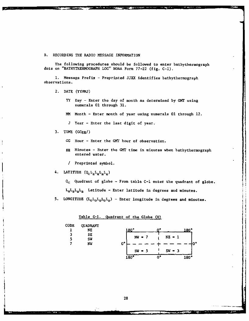
4. LATITUDE (QcLaLaLaLa)

Qc Quadrant of globe - From table C-I enter the quadrant of globe.

LaLaLaLa Latitude - Enter latitude in degrees and minutes.

5. LONGITUDE (LoLoLoLoLo) - Enter longitude in degrees and minutes.

Table C-1. Quadrant of the Globe (U)

CODE QUADRANT1 NE 1800 QO 1803 SEI5 SW NW 7 NE-7 NW 00 + 00

SW 5 iSW- 3

1800 00 1800

28

6. INDICATOR GROUP 88888 - Temperatures at significant depths follows:

BATHYTHERMOGRAPH TRACE READINGS

Surface Depth - Temperature (ZoZoToToTo )

ZoZ o Water Surface, 00 is preprinted.

TOT0T Enter the surface water temperature value (*C) as readfrom the BT trace to the nearest tenth of a degree. When

the temperature trace is unreadable in the first 10 metersenter solidi (///).

ZZTzTZTz This group is repeated as many times as necessary toadequately describe the BT trace.

ZZ For subsurface depth to 99 m enter in whole m the depthat which corresponding temperature values are read fromthe trace. Example: For 5 m, record 05; for 97 m, record97.

SPECIAL CODING INSTRUCTIONS

999NN NOTE: Always include a 999NN group before recordingdepths of 100 m, 200 m and each succeeding 100 m intervalsto termination. NN is coded as 01 for 100 to 199 m; 02for 200 to 299 m, etc. When the 999NN code is enteredmark out the ZZT zTzT z heading.

ZZ For depths between 100 and 200 m, 200 and 300 m, etc.,enter the tens and unit digits only. Example : for 101 m,record 01; for 256 m, record 56; for 375 a, recQrd 75.

TZTZTZ Temperature Group - Enter water temperature at depth ZZin *C to tenths of degrees. All temperature values ofless than O*C will be coded at 5TzT z (5 indicates that anegative reading follows).

00000 Indicator Group - Inserted after last ZZTzTZTz group onlyif last group is an ocean bottom reading.

RADIO All messages must terminate with the ship radio call orCALL aircraft squadron designator or the letters ACFT.

29

.1C. HOW TO ADDRESS MESSAGES FOR RADIO TRANSMISSION

Message addresses should be indicated and forwarded as follows

OBS METEO WASHDC - For all platforms other than Navy and under IOC,IGOSS auspices.

FLENUNWEACEN - For Navy sponsored aircraft and ship observationsin accordance with current Navy instructions.

D. INSTRUCTIONS FOR NAVY USE

BATHY messages will be transmitted with PRIORITY precedence,classified in accordance with the ship's movement. The heading onthe BATHY radio message is identical to the heading on any Navy message.

For example:

P 250015Z DEC 71FM USS BOSTONTO RUWJAGD/FLENUMWEACEN MONTEREY

BTUNCLASJJXX etc ..............

Navy ships, in addition to filling out the REFERENCE and RADIOMESSAGE INFORMATION sections, will fill in the Navy ship section inthe upper left corner of the log sheet as follows:

3-4. Enter first two letters of ship type in spaces 3 and 4,and remaining letters as appropriate in the next twoshaded unnumbered spaces.

5-7. Enter hull number in spaces 5-7; precede by zeroes if

less than 3 digits. If hull number is 4 digits, enterthe first digit in the shaded unnumbered space.

12-14. Enter last digit of current calendar year in space 12.

Enter two digit number of current month in spaces13-14; Example : August 1972 is coded as 208.

Navy aircraft, in addition to filling out the REFERENCE and RADIOMESSAGE INFORMATION sections, will fill in the Navy aircraft section inthe upper right corner of the log sheet, as follows:

3-4. Enter first two letters of squadron type in boxes 3-4.

(Exception VAW squadrons enter "AW").

30

5-7. Enter squadron number in spaces 5-7; precede by zeroes ifless than 3 digits (Exception: detachments enter "D"followed by detachment number).

8-11. Enter numbers and/or letters assigned to identify, withina squadron, each sortie of each aircraft.

12-14. Enter last digit of current calendar year in space 12.Enter two digit number of current month in spaces 13-14.Example: August 1972 is coded as 208.

Preprinted letters under some of the boxes are for data processingpurposes and are not of concern to the bathythermograph operator.

Navy submarines will fill out the RADIO MESSAGE INFORMATION sectionas follows:

In the Surface Depth-Temperature group (with 00 preprinted indepth group (ZoZo); enter 999 in temperature group ToToT o to indicatesubmarine observations.

31

Lil

e0

Nor)

U..4C-

NC O 0 0 I

L It 0 cm if) w

0-

S w W,W~ D L iJ 2 - 0 u

In p -z2> L

w C4

00

w

0 0

0 0 0 0 0 0 0 0 0 0In 0 In 0 n 0 In 0 In

(M') Hld3a

32

01 0

-7o coIWELJ

ix 0

0 .0

C,

1z1~ z

0 AE I.IL<-]Gc z tor~

.Zlr oz~-'.L o~ ..~o0~o o <.c

oww ~~- 0

-. f 4 L,

0zO0 0~0aI' -U

-( -'t - o 4 0 --j > 0 , >-

71 0 0'z0 - 2c

54

EV0 I' - I

00 . 0

zz - - -A -- -* ) - o - 0 -m

w 0

*3 3

Ieczr .0 A

*1

:4

I I

I

* r

34 I

I )

APPENDIX BEXAMPLES OF XBT MALFUNCTIONS

Under normal usage, approximately 5 percent of XBT probes will

malfunction for one or more reasons. Unfortunately, occasions arise

when nearly all of a batch of XBT probes fail because of improperstorage (high temperature, storage other than vertical) or old age(normal shelf life is 3 to 5 years). When failures occur, the analyst

* 1must recognize them in order to assure analysis accuracy. Higher than

normal failure rate will be experienced in strong oceanic frontal zones,

during heavy seas, and when the reporting ship is streaming instrumenta-

tion such as a VDS.

The following figures show a variety of XBT failures.* Completefailures are relatively easy to detect. Marginal failures are frequently

difficult to determine, particularly when taken in frontal areas. Whenin doubt, a second probe should be dropped as soon as possible to

validate the trace in question.

I

*A more comprehensive description of XBT failures is given in Kroner, S.M.and B.P. Blumenthal, Guide to common shipboard expendable bathythermograph(SXBT) recording malfunctions, Naval Oceanographic Office Reference Report21, Bay St. Louis, MS. (In preparation).

35

Ilk

0 0 0 0 0 0 Fo- 0--4 74c 0 If)o

0~00 0 0

- -

0

1 -0 0 0

w~ (D

CL~ 0 -

x

Co

-0

4)

3co

q- -

in0 n 0 IW4 :: W)li t a II1w

lil

f i l,.A..oo

0

+44 - - 4- -t -IE

1 f 111 1 1

I I I ; I , - V0

cc

x CL

37

6~- n- 6

0 1000 n-c

f i l 11 1 1 . f l

4)4) 4;

:Ckj:U C0

+ 1-4-

II-:4~ 41

I T 14)

38

0I0n 0 0 0o 0 0nwqt

CL I 1 1 1 1

-too

EL

I aI0 -

II

00

39

0 L 0.L 0 n.0 0 0 In

IaIn

0~0

40I -c

4-4-

9La

xEwC

+ t +

in C

40

0 0 0 0 0 0 0 ;

FO: # I T

aII -.L

(/)

1-7 CY

Ilt-

" I

41

z 0I I-. T

CLCLEl

42v

10 0 n 0 0

hfi

hi C

IF I

L-

CLC

Is *

I~ in

I43 I I

I t1 I

0 0=O 0 .0 0 0, 10 0 0

F 0 An 0 :: &) 0. ul), 0 i

C~i CV

0

C4

IL

tv. 44

cc In.

(r oi i

0>

UJ 0)Ga-C

IGa

cl 00v

.0>

0 o

w -401

If~ ~ I-,--C

1 0

LU C

_LL.4 I0-L

00

45

- -- 0

4:0~~~4 00

0 03c

00..

w - --i -,cO

C-

~ EF

46

AAI4 mbed&&* 1 .11,111, a .. . ......

APPENDIX C

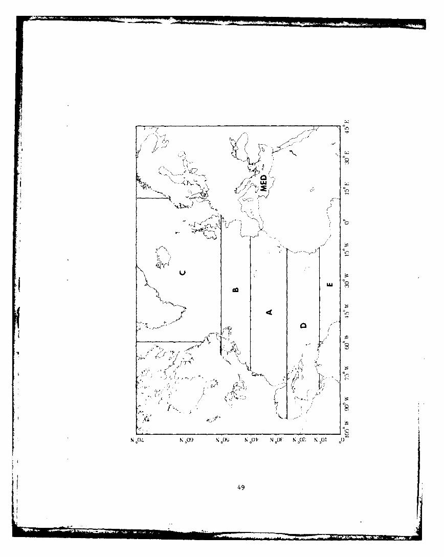
WATER MASS CRITERIANORTH ATLANTIC OCEAN/MEDITERRANEAN SEA

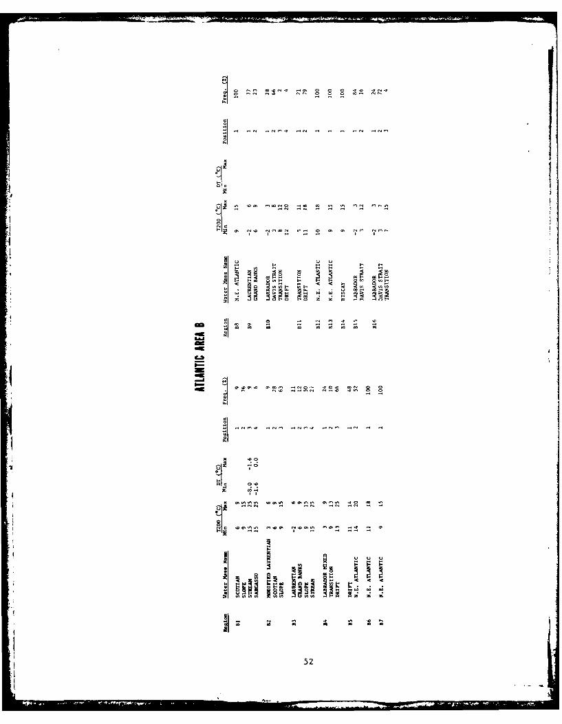
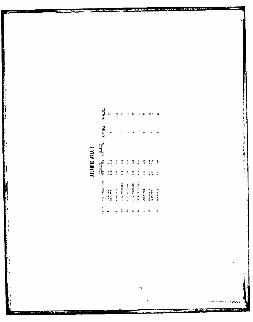
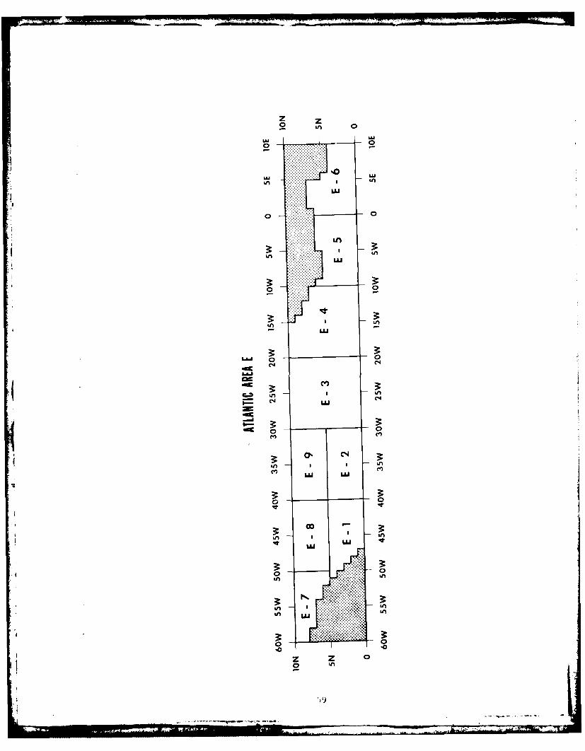
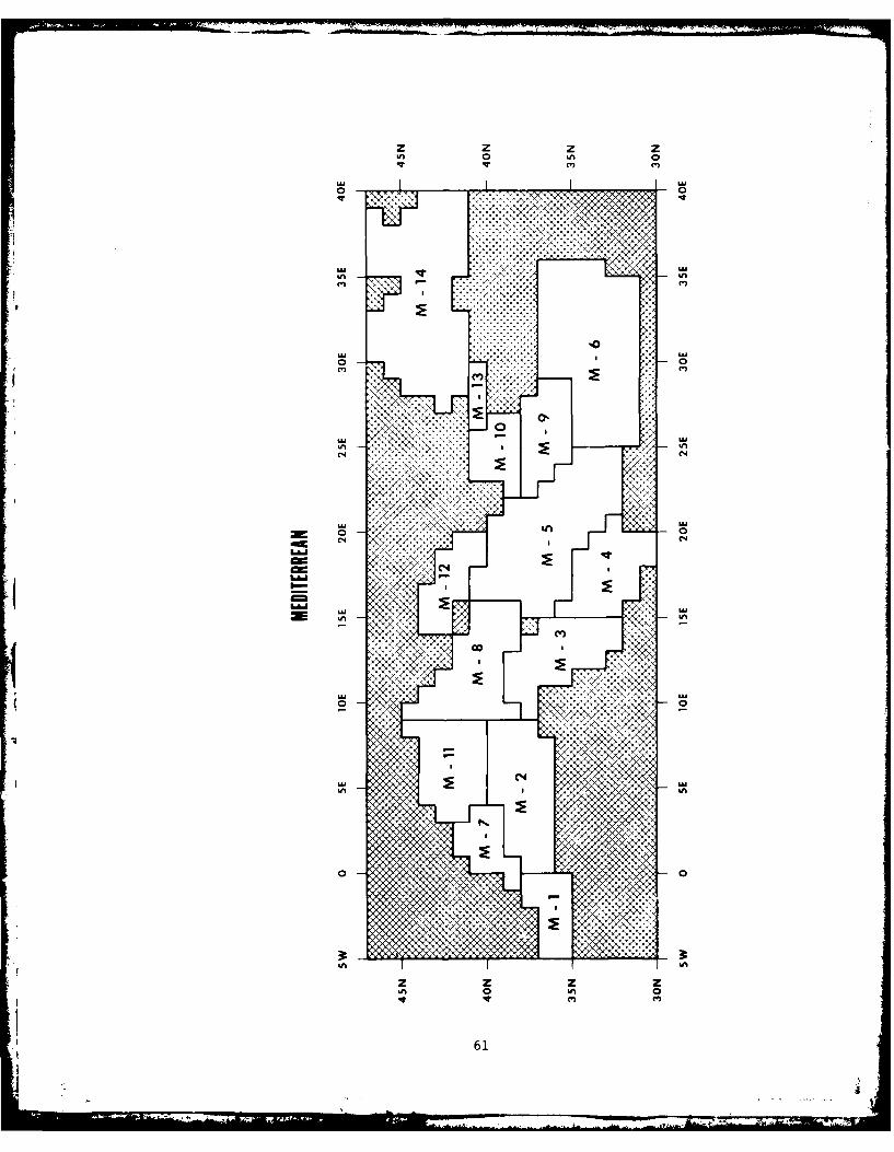
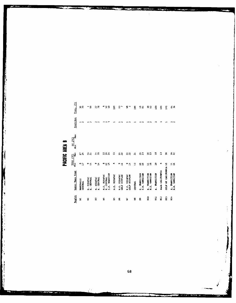
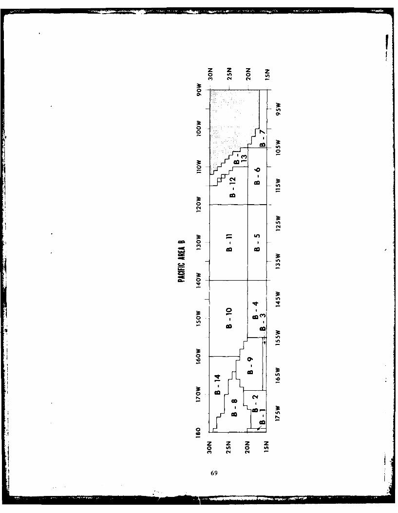
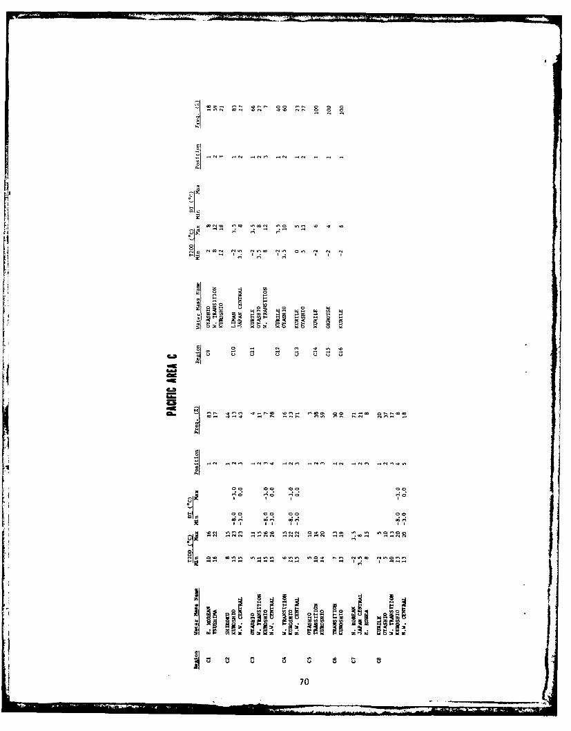
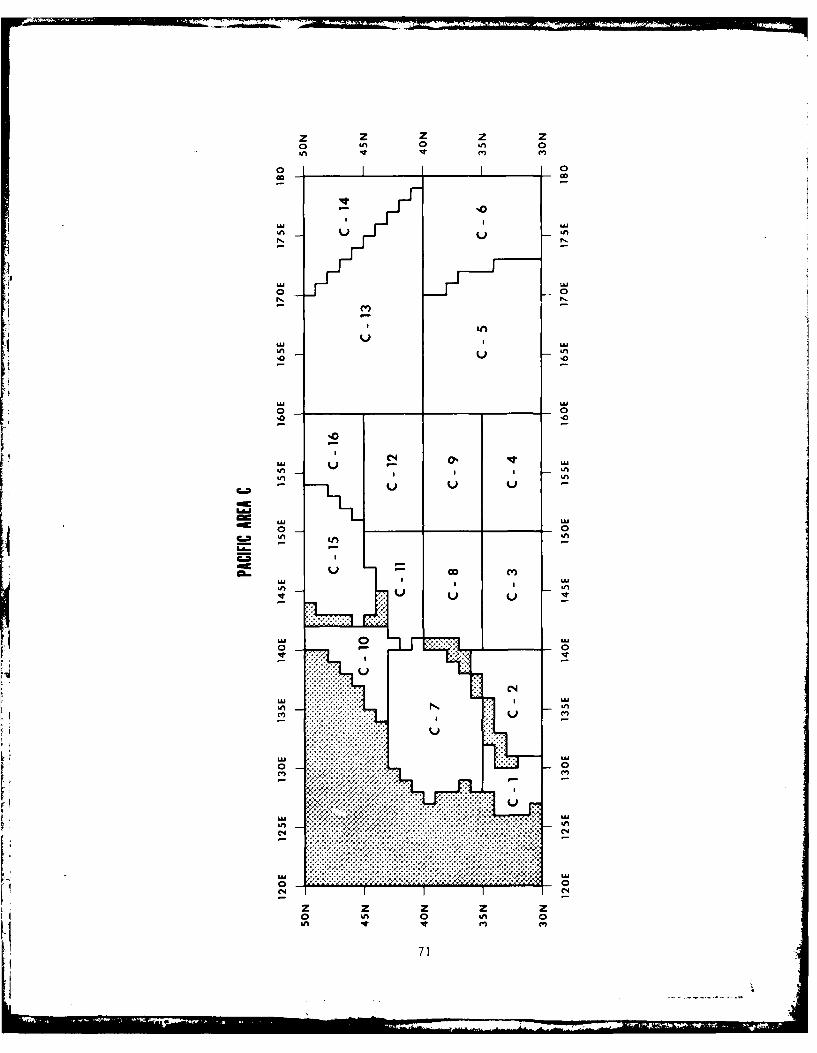
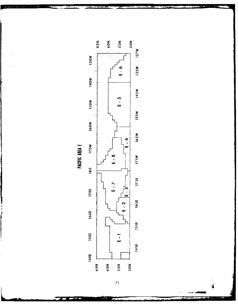
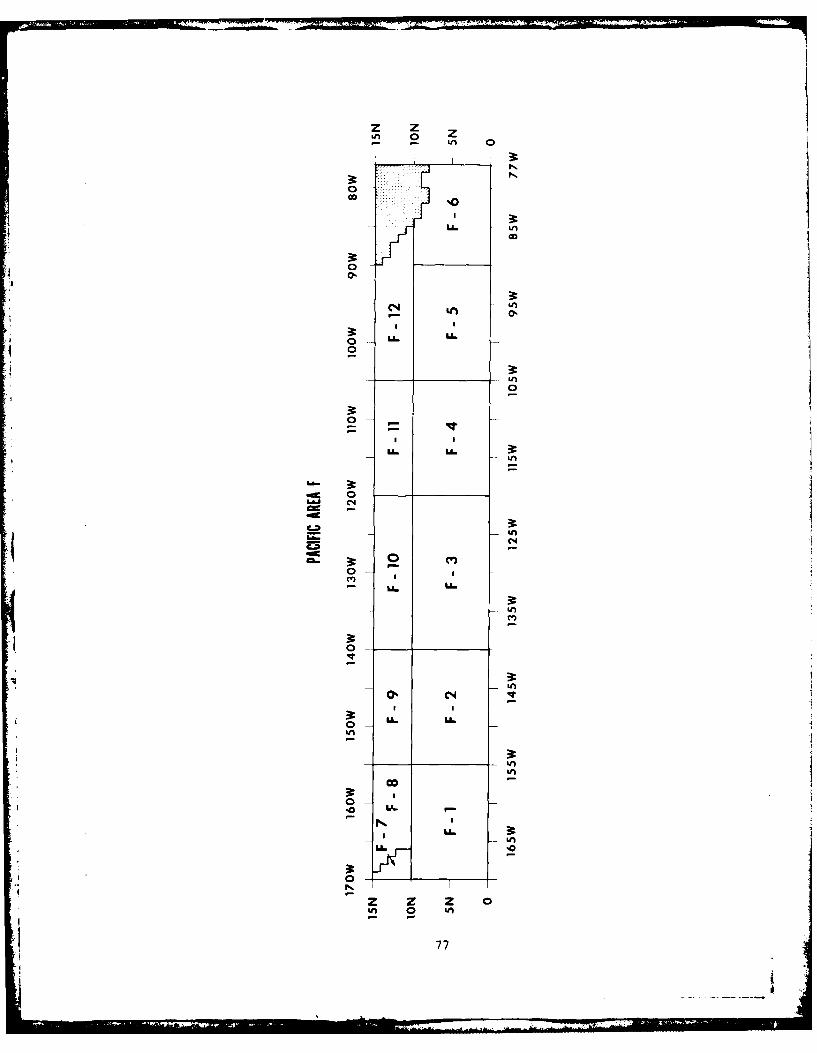
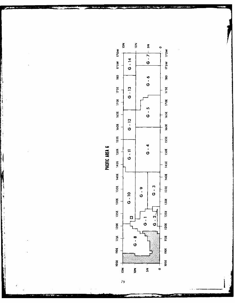
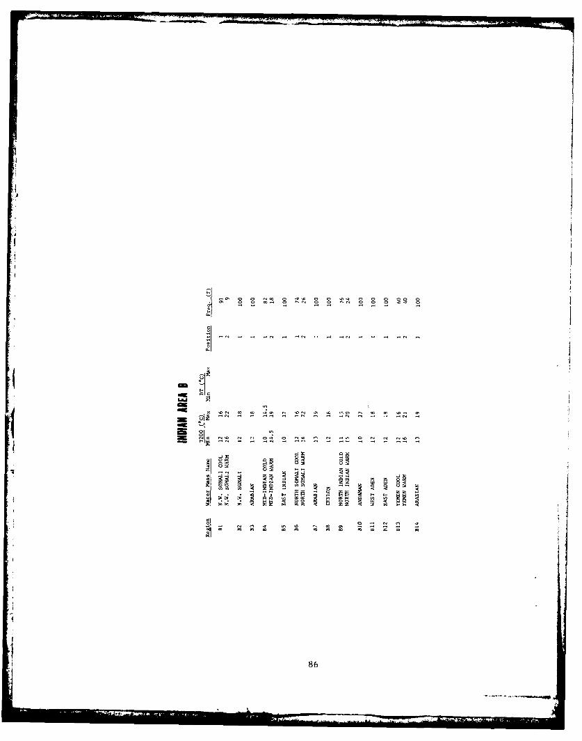
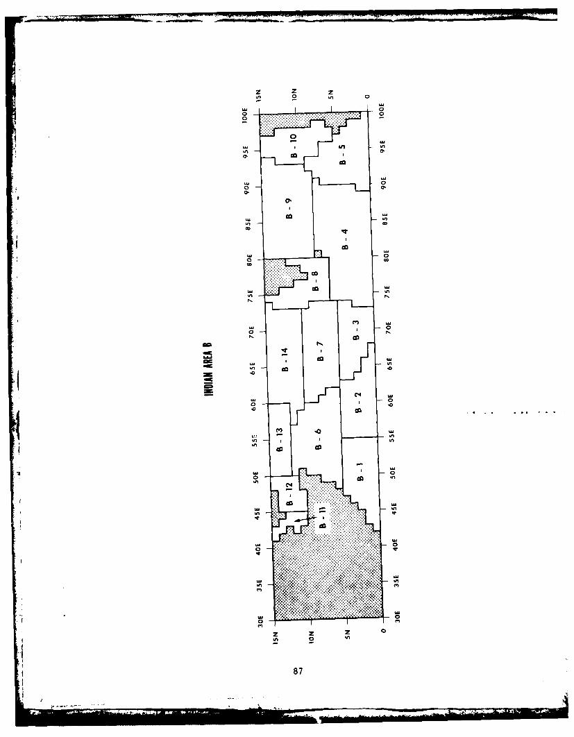
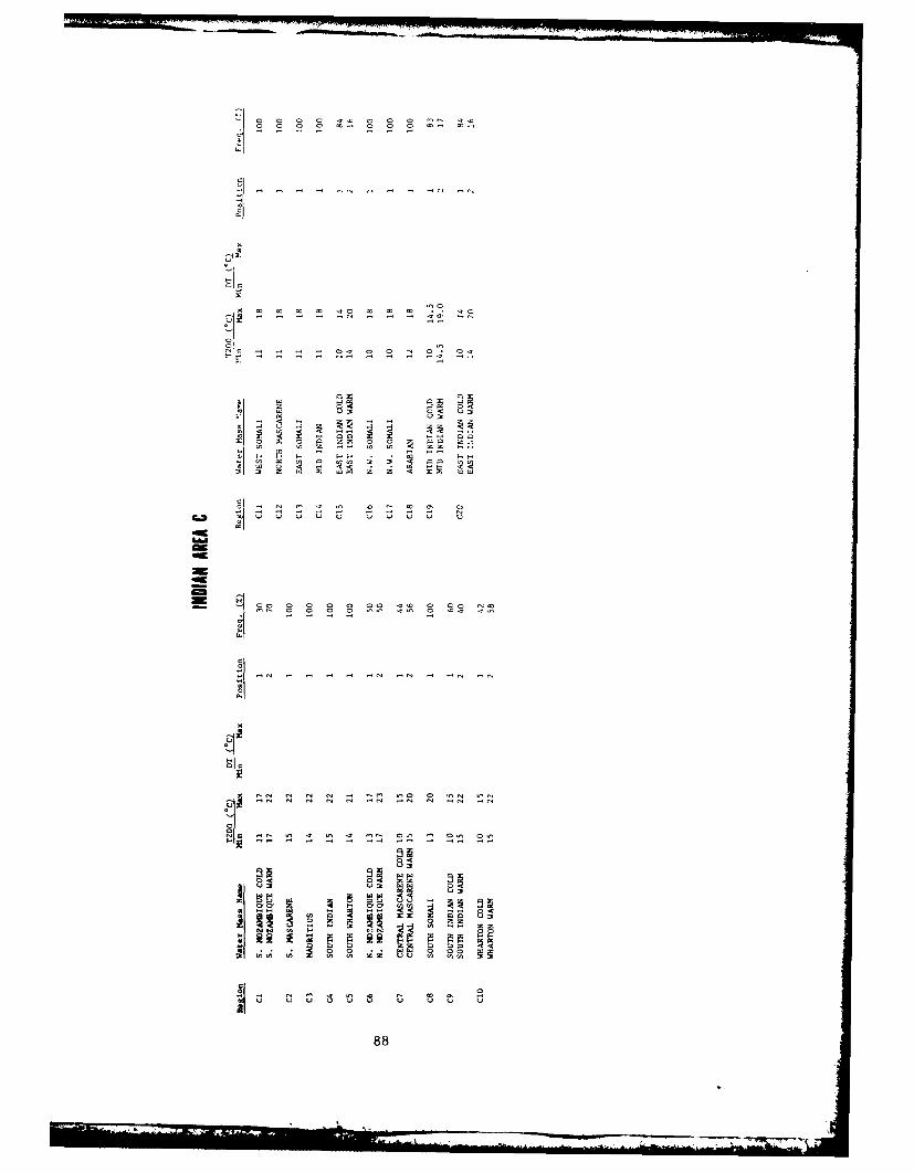
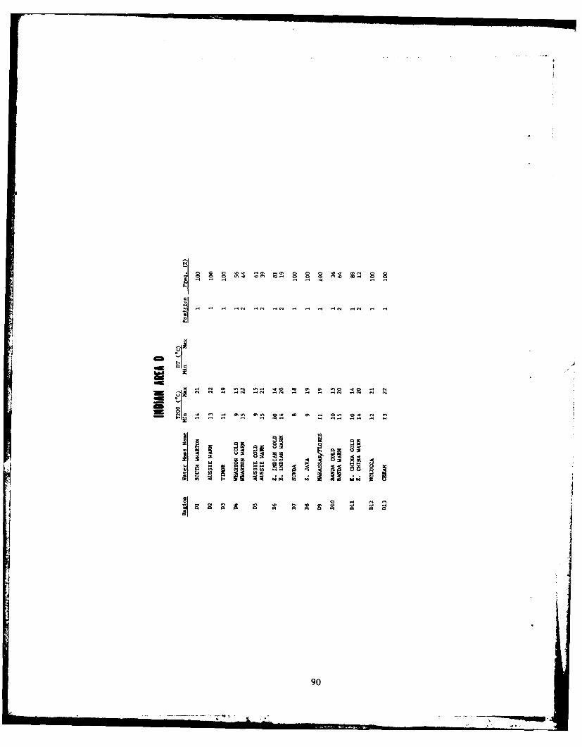
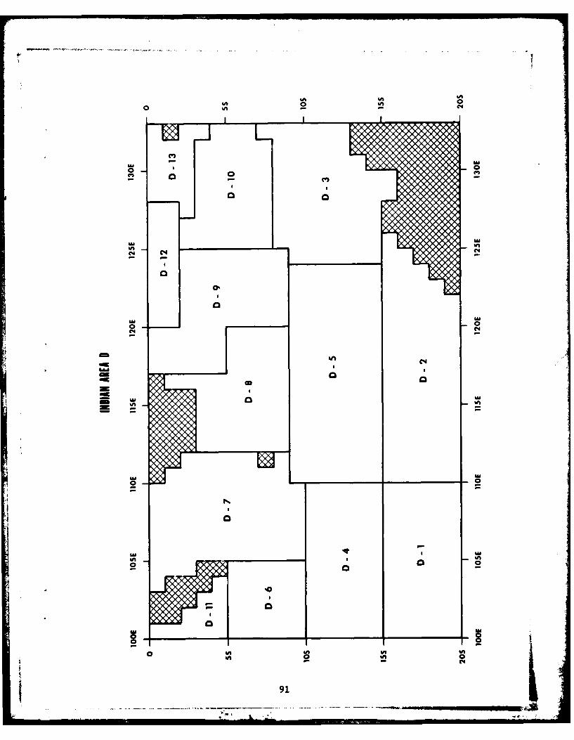
This appendix presents area definition and the thermalcharacteristics of each water mass within the file for the NorthAtlantic Ocean and the Mediterranean Sea. Subsequent appendixescover the North Pacific and the Indian Oceans. Each segment isdivided into areas designated by letter (e.g., Atlantic A). Withineach segment, geographic regions of similar oceanic properties aredesignated by number (Atlantic All). Although as many as five watermasses may occur in each region, most regions normally contain oneor two. For example, region All includes three water masses:Southern Slope, Stream, and Sargasso. It should be noted that

large water masses, such as the Sargasso Sea, may cover severalregions. Regions, water mass names, temperature range at 200 m(temperature filter), temperature difference between 200 and 300 m (DT)where applicable, file position in the ICAPS water mass file, andfrequency of observation of each water mass are provided in tabularform for each segment.

Water mass classification should be made initially usingtemperature at the 200 m level. When two water masses have similartemperature characteristics at this level, the temperature differencebetween 200 and 300 m (DT) should be used as a tie breaker.

CONTENTS

Page

Locator Chart ....... ..................... 49

Atlantic Area A ....... ..................... 50

Atlantic Area B ....... ..................... 52

Atlantic Area C ....... ..................... 54

Atlantic Area D ....... ..................... 56

Atlantic Area E . . . . . . . . . . . . . . . . . . . . . 58

Mediterranean Sea ....... .................... 60

47

48

__________________________________________________________________________________ a- '

-I V ~

N~N~ ~ -

N-~*ff-~.~-~,7 LU

(2 a

-..--'

*1 -4~.

V

LU

4' 0

~~~LI<A K ~

jfk ) -.

9 ~ AO 'VIs

1 7

4-' $

ire ~ a

-; (4

1.zNOL N0O~) N0O~., N~0Ot' N0OF NOc. \Ot ~()

49

g g a-*.r~~.~--~.ra C 00 a -C

C'

-~ -a cc

Cc Cc Cc ON

a', .1~ C C C C 0 ~a~aa~.flS~ C C C C Cf -I I -

El I- C C IL C CC, C < F- C CZ C F-. - IL F' F-

II .4.4 4 .4 .4C U a aC F-. F-F-CC C F- I- I- C CC, O 7Z~CC 0 0 U IL IL IL C C Q<

- C - - A F- - C 'C 'C - - - F-- .4 2 .~ a a Ta TIC F- .-J .4 .4 0 U F-C.......-U~'C 4JC,~< <F-IL

* *. - 4 01 01 tr .4 00CC CCC <.-..4 CO in CO Z 4 .4C

~ ~

- ~I CI~ 01.tO.C C.I'~ 0 -. ,.C CCC C C C cCOCC CCC C- CIa ~ILC . N C Nr C 0 C C NC CC C

.CN -

*1

x .rc .rc .rC .rc .rc .rC25 25 25 25 25 -c

F-Cc CC CC or cc Cc cc

~2 o2 ~2 ~-.II II II II I II

C ILIa~flIa .r.rC 'C NC-lCd C CIaILIL.CCIL

F-

C 0~ III.

01 14 U U LC 01.414 F- F- 4

C 0 014 14C 411C - C CC III~ .4 .. J~C 5~ F-C, F- .401 .4C, F- .4Ia CCU 7 7 .44 IC C

.~ ~ C 4C, ~ .~ .~C, UC, a -a a aCC C, ICCC, CCC, C,

0 - C-I C'

4

50 I?

C - 'I--.

z z z zo &M 0 0~

o N~o

:4 C4 4.-

NN

I n

0--

m.c

C=4 4m 0 0

C4

N 00

~ Sn N

_C 43cS0---- -

~Go

z SnLM 0 L

51

-0 - r- - - - -~ - % - n - 0%- --

9 1-

... ... ....% - 0 0 0 Jfl rfI

-. 1 I I - - -

18I-un -

52 ~ (0

z z z0 An 0tn

An Letn

01

I.,

LM InIAf

0 0

In 1 I - 4n

'00

0 0 0An In

Le) in n

An LM

o 0

.0 co a

0 An 0

53

:1

-i Ci

- Hr ii i ai i

i .'0asza .H: 2 -i J m52*jj j

*1 54

z z z z z

o o 0

'LI

UUL

0N N0

4n tn

CC4 N~

In Iin

0

&MVL 0

'7-

Lai

K0 Q o IM4

00 000 0 0 00 00 56

z z z zkmI 00

0~

N C

C41 C.,

~ 0 0

o 0

I'n

0 0

0 0o

kn U

100

co0

N A

U, OD

'n X 0cc

0 0l.... ....

01 01

57

* ~ ~ '0 0 ~0-1 C

4 222222 '0 2

I.'.'

-CO 00 0 0 C' 0 0 0 00 0

~ .~ '0 '0 ~'. '0 '.7 '.±-.~

=- 2

H~ ~~v; - - 0) '0<~ 0

- NO 00 0 0 0 0 0 0 00 0

0

- C-. o- -F F ~ I-' C- -

~C 0)0~ ~ g g - ~C- a-'C 0 0 0

S -' - 0 3-' 0~ 0& 0 La 0 00' 0S - 0. 0) ~t 0) a., - '-. La F-

-4 '.00)0 0 '0

*1 58

6 - L 0

LU LU

LUL

LU LULn

LU

00

* In

LA *: LA

L&LU

C=:

-n LU

33

- LA Ln

Cl" LUJ LU

0 0

c4.

1: -Ln LA

LU LU

on LMLAM*

0 .0

0 LA

f 6

f~~~ -I d Y2ZC-

<C _ <_ 22 2 2 . 2 " - 2 2

" C: 7 7 7 - :

bO0

Ln0 In0

100

;41

b&Jj

20 0

IC=

Lu 61

62

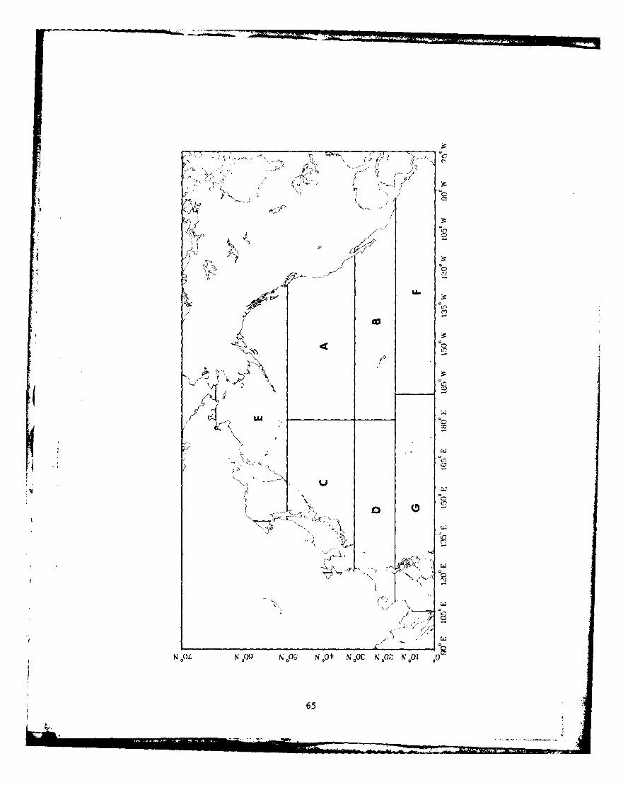
APPENDIX DWATER MASS CRITERIA

.5 NORTH PACIFIC OCEAN(See Appendix C for explanation)

CONTENTS

Page

Locator Chart.........................65

Pacific Area A...........................66

Pacific Area B...........................68

Pacific Area C...........................70I

Pacific Area D...........................72

Pacific Area E . . . . . . . . . . . . . . . . . . . . . . 7

Pacific Area F...........................76

Pacific Area G...........................78

63

.9

.1

)

I

I

* I

* i

I 64

*1

.. . ,

/5 - <p K-~ C

1'!

00

*11

II

a-

-

66

z z z z0 in 0

- . ..... ... ..... X.. X

%0

.. .. . .. . .. .

In %n

0; 0

-m-o

In U,

0 '0

00

N

z z z z z0 in 0 i

67

I2

00 .-4O~ CNO ~ 40 0C, n C O~4 04 C 0 C *A~~~~~~~~~~~~ * fr C Ch fC 0 C z~Q 0 0 0 C

m le w 1 2; 4 L 12 m 4

I.'68

z z z zC.) C~4 CN

0----n0..

9n

0%C4 1

ac -

S-2.

m~ 0-

an

0%

an

0%

00

Os

0'

o z0 A -LM 0* C

69n

Mllr-

C-2

I-I

I An sg -..

~0~

z z Z Z z

0 0 n

0 II0

uj u

LUUL

0 N

n In

UL

0C- L

71V

.01

00 'Cto ~4 OtCO' ~ 0 0

nr1 C! 1-i C!lC

5 5u

0

to 0072

z z Z zN in 0

0U 0

0 C2

LU LO LU

LA L

'00

L" L

'0

LU La

LU2

LU L"

LA Ln

LnU

C-

La-

LU L

IILU

LUi 0

LUn

Ln

UA LU

zz 2 Z z0 LA 0

73

~1

.4

o C C C C C C C

C 0 0 0 C C

LIJO2~

~ .. .~ ~ 'C~~1I 'a-~~lo T CI C C 0 Ia

C

I. 1-. .1 C (C

-I'C CC C C

74

z z z zLn 0 kn 010 10 LA Ln

01

00

LAJ

0u

10

0.

LALAcc.

LAn

CL. 0

LAJ I LY

0 L

LA

1 0

LU Lu0

- 00

Lu N

0

LU

LA

LUcv

0 n L

-40 0 in LA

750

I

C'J~ C C 0 Q .flU*~ ~ r~nc~ C r.r, 0'~-~C- ~N t-.e4 X' C O~ 0'

S 4 40 40 fl '0 C '0 .4.4 ~ C-4 '0 4C4 404

__ C C 0'-4 CO' Ce4C C C-S 0~t

__ CO 0'~ 0' 0' -

0 0'

0' U

B S~ a a~ aCS S _ 4. 4.0 4.0S. c-r.2 4. _ aw w4) U U . I CU .04 * *4 .4.4. 4) 4) 0' 4) "~ "-~"I .40) 0').) 0' 0' 4.C) * .4

4. 4.~ 4. 4. 4. 4.4. 4.

-I

76

z z

00

LL.

- - LA.

LaLM

ac 0-= -

- U. LA

U,

0C14

LI

U.. UL.

00

61U

07

........ ~ ~ ~ ... .. .. .. .. .

II

.. 1

---- . .t. .4 .t. .* . -4 --- 4 ------

4', <. C 0 .

7. w

78

z z

0- 0

I UIn

0 0

C-D,LU w)

a-I

'ILU uJ

0 C 0c2~

Lu u

0 0

Lm LUGoU'

o 0

- In

iI

if

I

80

APPENDIX EWATER MASS CRITERIA

INDIAN OCEAN(See Appendix C for explanation)

CONTENTS

Page

Locator Charts. ........................ 83

Indian Area A .................. ....... 84

Indian Area B .................... ..... 86

Indian Area C .................... ..... 88

4 Indian Area D .................... ..... 90

81

1 82

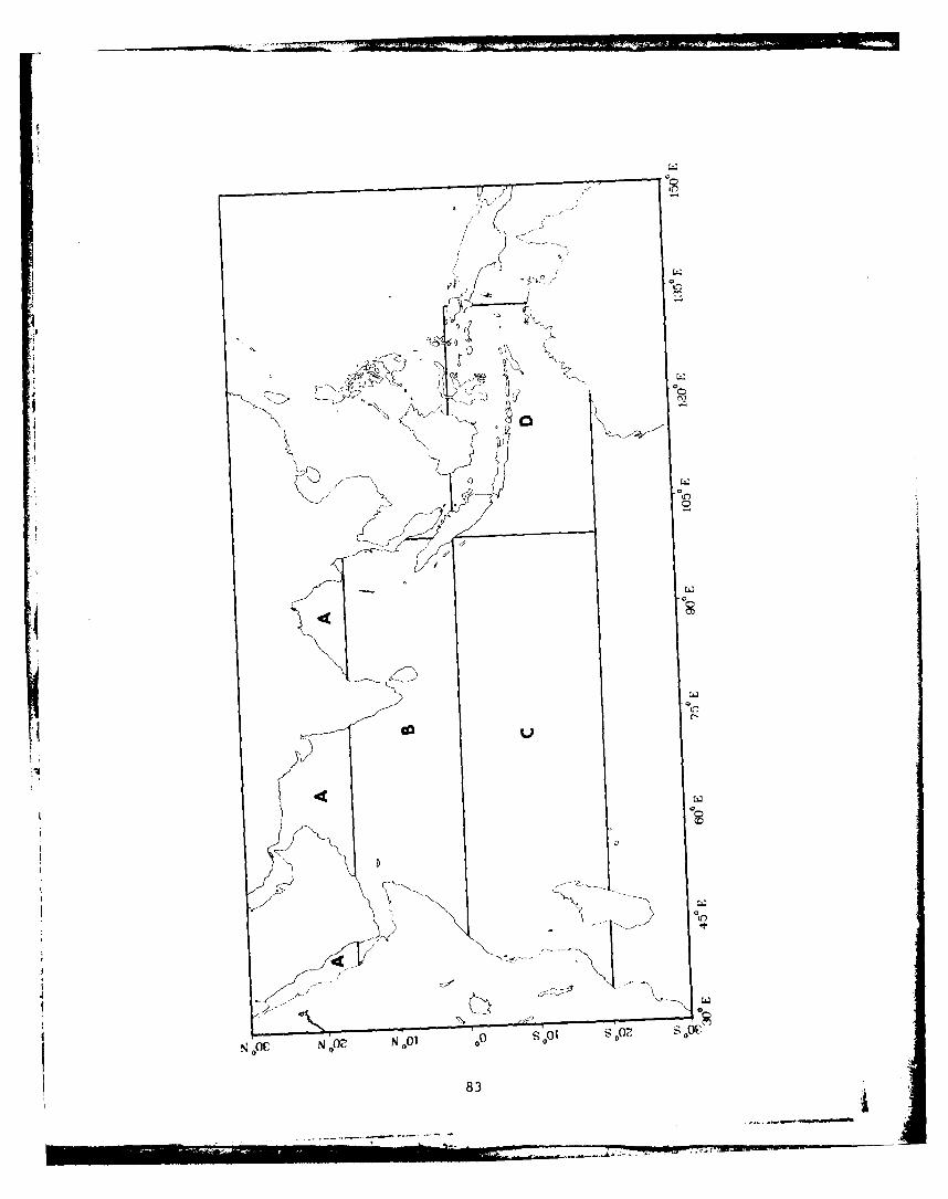
is~

N "pc N oz N .0

~~83

z Cz 0 0 H

-84

La 0

o 0o

0

Ln Lm

''1

LLA

. *.. .... .N .. .. . . .

L

..... .... . N

(n _4 LA m

=8

Idf

~ z -

86

Ln 0 0n

LU An

Ol cc

00

00

000

coA

0

0.

C.14

0

C.) L

n1 87 c

0 0o 0 0 - a0 0 co • - "

- - - - - - - - -- --

Z Z

mc

Qa M

44~ l

0 '"

0S .4 - ,80

OCEAN0GRAPHIC ANALYSIS MANUAL FOR ON-SCENE PREDICTION SYSTEMS U)

A Y '18 NA A FAORP FICEHT TTO SFIEEEEEEEEJ0 M

nin282 1112.53 2O

1111111'1'l18fljf:.25 14 HII=LJ-

mi OPY p H ll(, f I H R

6n 04

o

w 0 MA

U' C4 - U

w a,

ini

o 0

go

sman.

UU

a c

0'

aM --- I U.

,aa

IN

M M

0o 0

sm

Inn

on 0

39

4 4

I

'n t 'CC 0 •

'O# 0 '-4~ 0 0 ~ "-8

'4 -.4 - - -4_

C9

In In0!

IM

'U 0

- I"

Sa

r 00

00

-0

91

I I I InIIIIIII M

. ... ... I I

92

APPENDIX GGLOSSARY OF ACRONYMS

ASW - Antisubmarine Warfare

BATHY - Bathythermograph data encoded for transmission

BB - Bottom Bounce

BLG - Below-layer Gradient

BT - Bathythermograph

CZ - Convergence Zone

DR - Dead Reckoning

DT - Temperature at 300m minus temperature at 200m,

DTG - Day/Time/Group

FLENUMWEACEN - Fleet Numerical Weather Central, Monterey

ICeAPS - Integrated Command ASW Prediction System

ILG - In-layer Gradient

IR - Infrared

NWPCB - Naval Warfare Planning Chart Base

SLD - Sonic Layer Depth

SOA - Speed of Advance

SST - Sea Surface Temperature

TL - Temperature at the base of the below layer gradient

TSLD - Temperature at Sonic Layer Depth

T200 - Temperature at the 200-m level. Temperature at anylevel has a prefix "T" followed by the depth.

XBT - Expendable Bathythermograph

93S 4. t

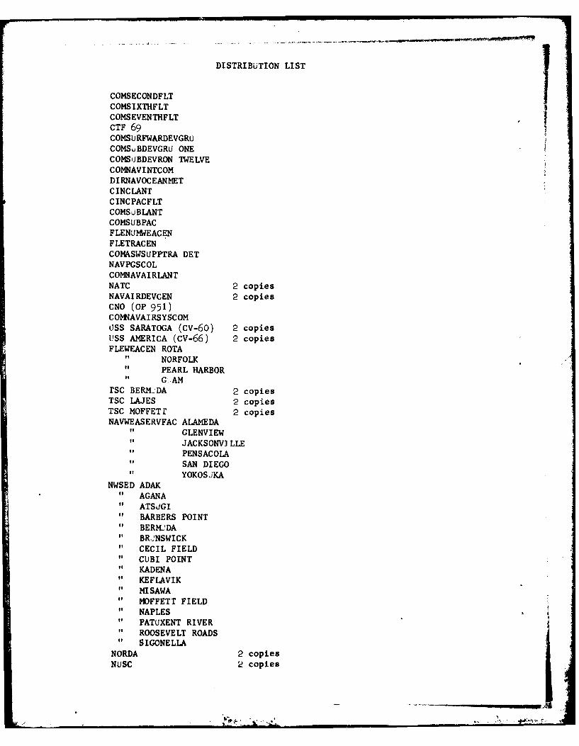
DISTRIBUTION LIST

COMSECONDFLTCOMSIXTHFLT ,

COMSEVENTHFLTCTF 69COMSU RFWARDEVGRUCOMSu BDEVGRU ONECOMSUBDEVRON TWELVECOMNAVINTCOMDIRNAVOCEAN MET

CINCLANTC INCPACFLTCOMSjBLANTCOMSUBPACFLENUM-EACENFLETRACEN

COMASWSUPPTRA DETNAVPGSCOL

COMNAVAI RLANTNATC 2 copiesNAVAIRDEVCEN 2 copiesCNO (oP 951)COINAVAIRSYSCOMUSS SARATOGA (CV-60) 2 copiesUSS AMERICA (CV-66) 2 copiesFLEWEACEN ROTA

Is NORFOLKof PEARL HARBORof G'.AM

rsC BERMDA 2 copiesTSC LAJES 2 copiesTSC MOFFETf 2 copiesNAVWEASERVFAC ALAMEDA

to GLENVIEWgo JACKSONVILLEof PENSACOLAIt SAN DIEGO"1 YOKOS JKA

NWSED ADAK" AGANA" ATSUGI" BARBERS POINT" BERMJDA" BR.JNSWICK" CECIL FIELD" CUBI POINT" KADENA

KEFLAVIKMISAWA

" MOFFETT FIELD" NAPLES" PATUXENT RIVER" ROOSEVELT ROADS" SIGONELLA

NORDA 2 copiesNUSC 2 copies

UNCLASSIFIED

SECURITY CLASSIFICATION OF THIS PAGE (lWhn Date Eat',e4)

READ ISTRUCTIONSREPORT DCUMENTATION PAGE BEFORE COMPLITING FORM1. REPORT NUMBER 2. GOVT ACCESSION NO S. RECIPIENT'S CATALOG NUMBER

NO0 RP 20

4. TITLE (and Subtitle) S. TYPE OF REPORT & PERIOD COVERED

Oceanographic Analysis Manual for On-scenePrediction Systems

S. PERFORMING ORG. REPORT NUMBER

7. AUTHOR(*) 1. CONTRACT OR GRANT NUM89RO)

Alan Fisher, Jr.

9. PERFORMING ORGANIZATION NAME AND ADDRESS 10. PROGRAM EL.EMIENT. PROJECT. TASK

AREA & WORK UNIT NUMBERS

U.S. Naval Oceanographic OfficeNSTL StationBay St. Louis, MS 39522 ..

11. CONTROLLING OFFICE NAME AND ADOWESS 12. REPORT DATEMay 1978

13. NUMBER OF PAGS93 (Incl 6 appendixes)

14. MONITORING AGENCY NAME & ADORESS(ii'dltfermat from Cotrollg Office) IS. SECURITY CLASS. (of thl ripo )

UNCLASSIFIEDIs*. OECL ASSI PICATION/ DOWNGRADING

SCNEDULE NIA

S4. DISTRIBUTION STATEMENT (of this Report)

Approved for public release, distribution unlimited.

17. DISTRIBUTION STATEMENT (of the bstract uttered In block" 0, It different hem Repet)

18. SUPPLEMENTARY NOTES

19. KEY WOROS (Cetinue on reverse side it noceeev atd IentI by block nmbr)ICAPSOn-scene prediction Sound speed conversionOceanographic data collection Water massesOceanographic data analysis

Oceanographic data interpretation20. ABSTRACT (Conftnue an reverse aide It neceesmy arid Ientl& by block unuabm)This report is intended to acquaint Naval personnel having minimal

oceanographic training with techniques used to prepare an oceanographicanalysis as an initial step in acoustic performance prediction. Oceanographicdata are discussed with particular emphasis on the quality control ofexpendable bathythermograph (XBT) data. Oceanic features, such as watermasses and boundaries, are reviewed to provide background information necessaryfor meaningful analysis. A sample analysis is made to assist the inexperienced.anal st in methods used. Finally, the process of selectini data representativeDO ,Fo 1473 fmITION OP I SOV ls is OBOL8ETE UNCLASSIFIED

_______ _ o_~o_-o__ -__o_ _ SeCURITY CLAWSIICAT op Tolls P s (WA, N. uemO" -- • I II ~ ~ ~~~~ i J .. 4. l: . 1 II ..... r .. .

UNCLASSIFIEDL.LUR1TY CLASSIFICATION OF THIS PAGE(Whem Date ntered)

ABSTRACT continued:

of each water mass for input into acoustic models is discussed.

I

S .

SECuRiTY CLASIPICATION OF T"IS PAEhl Dat. er Won

ILMED