Oliver Stegle and Karsten Borgwardt: Computational Approaches for Analysing Complex Biological Systems, Page 1 Linear models Oliver Stegle and Karsten Borgwardt Machine Learning and Computational Biology Research Group, Max Planck Institute for Biological Cybernetics and Max Planck Institute for Developmental Biology, Tübingen
Transcript
Oliver Stegle and Karsten Borgwardt: Computational Approaches for Analysing Complex Biological Systems, Page 1
Linear modelsOliver Stegle and Karsten Borgwardt
Machine Learning andComputational Biology Research Group,
Max Planck Institute for Biological Cybernetics andMax Planck Institute for Developmental Biology, Tübingen
Motivation
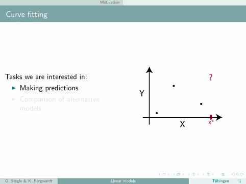
Curve fitting
Tasks we are interested in:
I Making predictions
I Comparison of alternativemodels
X
Y
?
x*
O. Stegle & K. Borgwardt Linear models Tubingen 1
Motivation
Curve fitting
Tasks we are interested in:
I Making predictions
I Comparison of alternativemodels
X
Y
?
x*
O. Stegle & K. Borgwardt Linear models Tubingen 1
Motivation
Further reading, useful material
I Christopher M. Bishop: Pattern Recognition and Machine learning.I Good background, covers most of the course material and much more!I This lecture is largely inspired by chapter 3 of the book.
O. Stegle & K. Borgwardt Linear models Tubingen 2
Outline
Outline
O. Stegle & K. Borgwardt Linear models Tubingen 3
Linear Regression
Outline
Motivation
Linear Regression
Bayesian linear regression
Model comparison and hypothesis testing
Summary
O. Stegle & K. Borgwardt Linear models Tubingen 4
Linear Regression
RegressionNoise model and likelihood
I Given a dataset D = {xn, yn}Nn=1, where xn = {xn,1, . . . , xn,D} is Ddimensional, fit parameters θ of a regressor f with added Gaussiannoise:
yn = f(xn;θ) + εn where p(ε |σ2) = N(ε∣∣ 0, σ2) .
I Equivalent likelihood formulation:
p(y |X) =N∏
n=1
N(yn∣∣ f(xn), σ
2)
O. Stegle & K. Borgwardt Linear models Tubingen 5
Linear Regression
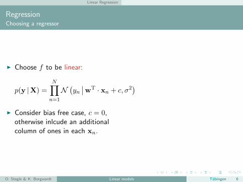
RegressionChoosing a regressor
I Choose f to be linear:
p(y |X) =
N∏n=1
N(yn∣∣wT · xn + c, σ2
)I Consider bias free case, c = 0,
otherwise inlcude an additionalcolumn of ones in each xn.
O. Stegle & K. Borgwardt Linear models Tubingen 6
Linear Regression
RegressionChoosing a regressor
I Choose f to be linear:
p(y |X) =
N∏n=1
N(yn∣∣wT · xn + c, σ2
)I Consider bias free case, c = 0,
otherwise inlcude an additionalcolumn of ones in each xn. Equivalent graphical model
O. Stegle & K. Borgwardt Linear models Tubingen 6
Linear Regression
Linear RegressionMaximum likelihood
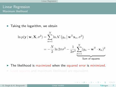
I Taking the logarithm, we obtain
ln p(y |w,X, σ2) =N∑
n=1
lnN(yn∣∣wTxn, σ
2)
= −N2ln 2πσ2 − 1
2σ2
N∑n=1
(yn −wT · xn)2
︸ ︷︷ ︸Sum of squares
I The likelihood is maximized when the squared error is minimized.
I Least squares and maximum likelihood are equivalent.
O. Stegle & K. Borgwardt Linear models Tubingen 7
Linear Regression
Linear RegressionMaximum likelihood
I Taking the logarithm, we obtain
ln p(y |w,X, σ2) =N∑
n=1
lnN(yn∣∣wTxn, σ
2)
= −N2ln 2πσ2 − 1
2σ2
N∑n=1
(yn −wT · xn)2
︸ ︷︷ ︸Sum of squares
I The likelihood is maximized when the squared error is minimized.
I Least squares and maximum likelihood are equivalent.
O. Stegle & K. Borgwardt Linear models Tubingen 7
Linear Regression
Linear Regression and Least Squares
y
x
f (xn , w )
yn
xn
(C.M. Bishop, Pattern Recognition and Machine Learning)
E(w) =1
2
N∑n=1
(yn −wTxn)2
O. Stegle & K. Borgwardt Linear models Tubingen 8
Linear Regression
Linear Regression and Least Squares
I Derivative w.r.t a single weight entry wi
d
dwiln p(y |w, σ2) =
d
dwi
[− 1
2σ2
N∑n=1
(yn −w · xn)2
]
=1
σ2
N∑n=1
(yn −w · xn)xi
I Set gradient w.r.t to w to zero
∇w ln p(y |w, σ2) =1
σ2
N∑n=1
(yn −w · xn)xTn = 0
=⇒ wML = (XTX)−1XT︸ ︷︷ ︸Pseudo inverse
y
I Here, the matrix X is defined as X =
x1,1 . . . x1, D. . . . . . . . .xN,1 . . . xN,D
O. Stegle & K. Borgwardt Linear models Tubingen 9
Linear Regression
Polynomial Curve Fitting
I Use the polynomials up to degree K to construct new features from x
f(x,w) = w0 + w1x+ w2x2 + · · ·+ wKx
K
= wTφ(x),
where we defined φ(x) = (1, x, x2, . . . , xK).
I Similarly, φ can be any feature mapping.
I Possible to show: the feature map φ can be expressed in terms ofkernels (kernel trick).
O. Stegle & K. Borgwardt Linear models Tubingen 10
Linear Regression
Polynomial Curve FittingOverfitting
I The degree of the polynomial is crucial to avoid under- andoverfitting.
x
t
M = 0
0 1
−1
0
1
(C.M. Bishop, Pattern Recognition and Machine Learning)
O. Stegle & K. Borgwardt Linear models Tubingen 11
Linear Regression
Polynomial Curve FittingOverfitting
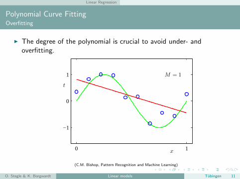
I The degree of the polynomial is crucial to avoid under- andoverfitting.
x
t
M = 1
0 1
−1
0
1
(C.M. Bishop, Pattern Recognition and Machine Learning)
O. Stegle & K. Borgwardt Linear models Tubingen 11
Linear Regression
Polynomial Curve FittingOverfitting
I The degree of the polynomial is crucial to avoid under- andoverfitting.
x
t
M = 3
0 1
−1
0
1
(C.M. Bishop, Pattern Recognition and Machine Learning)
O. Stegle & K. Borgwardt Linear models Tubingen 11
Linear Regression
Polynomial Curve FittingOverfitting
I The degree of the polynomial is crucial to avoid under- andoverfitting.
x
t
M = 9
0 1
−1
0
1
(C.M. Bishop, Pattern Recognition and Machine Learning)
O. Stegle & K. Borgwardt Linear models Tubingen 11
Linear Regression
Regularized Least Squares
I Solutions to avoid overfitting:I Intelligently choose KI Regularize the regression weights w
I Construct a smoothed error function
E(w) =1
2
N∑n=1
(yn −wTφ(xn)
)2︸ ︷︷ ︸
Squared error
+λ
2wTw︸ ︷︷ ︸
Regularizer
O. Stegle & K. Borgwardt Linear models Tubingen 12
Linear Regression
Regularized Least SquaresMore general regularizers
I A more general regularization approach:
E(w) =1
2
N∑n=1
(yn −wTφ(xn)
)2︸ ︷︷ ︸
Squared error
+λ
2
D∑d=1
|wd|q︸ ︷︷ ︸Regularizer
O. Stegle & K. Borgwardt Linear models Tubingen 13
Linear Regression
Regularized Least SquaresMore general regularizers
I A more general regularization approach:
E(w) =1
2
N∑n=1
(yn −wTφ(xn)
)2︸ ︷︷ ︸
Squared error
+λ
2
D∑d=1
|wd|q︸ ︷︷ ︸Regularizer
q = 0 .5 q = 1 q = 2 q = 4
(C.M. Bishop, Pattern Recognition and Machine Learning)
O. Stegle & K. Borgwardt Linear models Tubingen 13
Linear Regression
Regularized Least SquaresMore general regularizers
I A more general regularization approach:
E(w) =1
2
N∑n=1
(yn −wTφ(xn)
)2︸ ︷︷ ︸
Squared error
+λ
2
D∑d=1
|wd|q︸ ︷︷ ︸Regularizer
q = 0 .5 q = 1 q = 2 q = 4
QuadraticLasso
sparse
(C.M. Bishop, Pattern Recognition and Machine Learning)
O. Stegle & K. Borgwardt Linear models Tubingen 13
Linear Regression
Loss functions and other methods
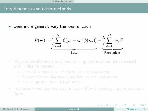
I Even more general: vary the loss function
E(w) =1
2
N∑n=1
L(yn −wTφ(xn))︸ ︷︷ ︸Loss
+λ
2
D∑d=1
|wd|q︸ ︷︷ ︸Regularizer
I Many state-of-the-art machine learning methods can be expressedwithin this framework.
I Linear Regression: squared loss, squared regularizer.I Support Vector Machine: hinge loss, squared regularizer.I Lasso: squared loss, L1 regularizer.
I Inference: minimize the cost function E(w), yielding a point estimatefor w.
O. Stegle & K. Borgwardt Linear models Tubingen 14
Linear Regression
Loss functions and other methods
I Even more general: vary the loss function
E(w) =1
2
N∑n=1
L(yn −wTφ(xn))︸ ︷︷ ︸Loss
+λ
2
D∑d=1
|wd|q︸ ︷︷ ︸Regularizer
I Many state-of-the-art machine learning methods can be expressedwithin this framework.
I Linear Regression: squared loss, squared regularizer.I Support Vector Machine: hinge loss, squared regularizer.I Lasso: squared loss, L1 regularizer.
I Inference: minimize the cost function E(w), yielding a point estimatefor w.
O. Stegle & K. Borgwardt Linear models Tubingen 14
Linear Regression
Regularized Least SquaresProbabilistic equivalent
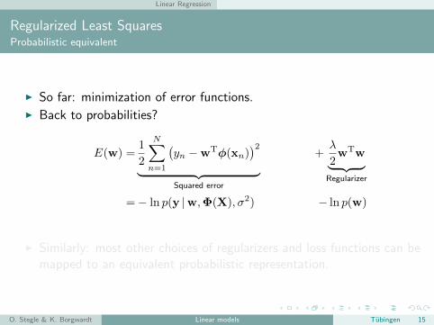
I So far: minimization of error functions.I Back to probabilities?
E(w) =1
2
N∑n=1
(yn −wTφ(xn)
)2︸ ︷︷ ︸
Squared error
+λ
2wTw︸ ︷︷ ︸
Regularizer
I Similarly: most other choices of regularizers and loss functions can bemapped to an equivalent probabilistic representation.
O. Stegle & K. Borgwardt Linear models Tubingen 15
Linear Regression
Regularized Least SquaresProbabilistic equivalent
I So far: minimization of error functions.I Back to probabilities?
E(w) =1
2
N∑n=1
(yn −wTφ(xn)
)2︸ ︷︷ ︸
Squared error
+λ
2wTw︸ ︷︷ ︸
Regularizer
=− ln p(y |w,Φ(X), σ2) − ln p(w)
=−N∑
n=1
lnN(yn∣∣wTφ(xn), σ
2)
− lnN(
w
∣∣∣∣0, 1λI
)I Similarly: most other choices of regularizers and loss functions can be
mapped to an equivalent probabilistic representation.
O. Stegle & K. Borgwardt Linear models Tubingen 15
Bayesian linear regression
Outline
Motivation
Linear Regression
Bayesian linear regression
Model comparison and hypothesis testing
Summary
O. Stegle & K. Borgwardt Linear models Tubingen 16
Bayesian linear regression
Bayesian linear regression
I Likelihood as before
p(y |X,w, σ2) =N∏
n=1
N(yn∣∣wT · φ(xn), σ
2)
I Define a conjugate prior over w
p(w) = N (w |m0,S0)
O. Stegle & K. Borgwardt Linear models Tubingen 17
Bayesian linear regression
Bayesian linear regression
I Likelihood as before
p(y |X,w, σ2) =N∏
n=1
N(yn∣∣wT · φ(xn), σ
2)
I Define a conjugate prior over w
p(w) = N (w |m0,S0)
O. Stegle & K. Borgwardt Linear models Tubingen 17
Bayesian linear regression
Bayesian linear regression
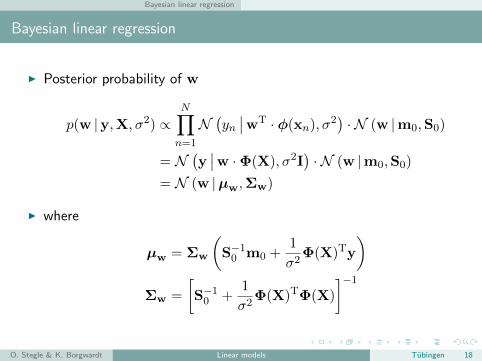
I Posterior probability of w
p(w |y,X, σ2) ∝N∏
n=1
N(yn∣∣wT · φ(xn), σ
2)· N (w |m0,S0)
= N(y∣∣w ·Φ(X), σ2I
)· N (w |m0,S0)
= N (w |µw,Σw)
I where
µw = Σw
(S−10 m0 +
1
σ2Φ(X)Ty
)Σw =
[S−10 +
1
σ2Φ(X)TΦ(X)
]−1
O. Stegle & K. Borgwardt Linear models Tubingen 18
Bayesian linear regression
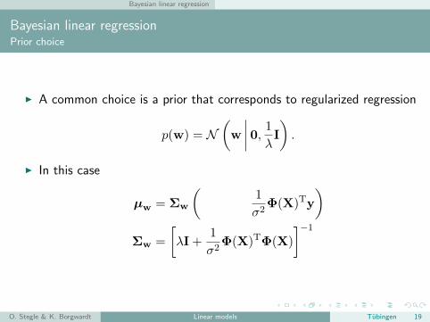
Bayesian linear regressionPrior choice
I A common choice is a prior that corresponds to regularized regression
p(w) = N(
w
∣∣∣∣0, 1λI
).
I In this case
µw = Σw
(S−10 m0 +
1
σ2Φ(X)Ty
)Σw =
[S−10 +
1
σ2Φ(X)TΦ(X)
]−1
O. Stegle & K. Borgwardt Linear models Tubingen 19
Bayesian linear regression
Bayesian linear regressionPrior choice
I A common choice is a prior that corresponds to regularized regression
p(w) = N(
w
∣∣∣∣0, 1λI
).
I In this case
µw = Σw
(1
σ2Φ(X)Ty
)Σw =
[λI +
1
σ2Φ(X)TΦ(X)
]−1
O. Stegle & K. Borgwardt Linear models Tubingen 19
Bayesian linear regression
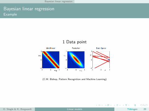
Bayesian linear regressionExample
0 Data points
(C.M. Bishop, Pattern Recognition and Machine Learning)
O. Stegle & K. Borgwardt Linear models Tubingen 20
Bayesian linear regression
Bayesian linear regressionExample
1 Data point
(C.M. Bishop, Pattern Recognition and Machine Learning)
O. Stegle & K. Borgwardt Linear models Tubingen 20
Bayesian linear regression
Bayesian linear regressionExample
20 Data points
(C.M. Bishop, Pattern Recognition and Machine Learning)
O. Stegle & K. Borgwardt Linear models Tubingen 20
Bayesian linear regression
Making predictions
I Prediction for fixed weight w at input x? trivial:
p(y? |x?, w, σ2) = N(y?∣∣∣ wTφ(x?), σ2
)I Integrate over w to take the posterior uncertainty into account
p(y? |x?,D) =∫wp(y? |x?,w, σ2)p(w |X,y, σ2)
=
∫wN(y?∣∣wTφ(x?), σ2
)N (w |µw,Σw)
= N(y?∣∣µT
wφ(x?), σ2 + φ(x?)TΣwφ(x
?))
I Key:I prediction is again GaussianI Predictive variance is increase due to the posterior uncertainty in w.
O. Stegle & K. Borgwardt Linear models Tubingen 21
Model comparison and hypothesis testing
Outline
Motivation
Linear Regression
Bayesian linear regression
Model comparison and hypothesis testing
Summary
O. Stegle & K. Borgwardt Linear models Tubingen 22
Model comparison and hypothesis testing
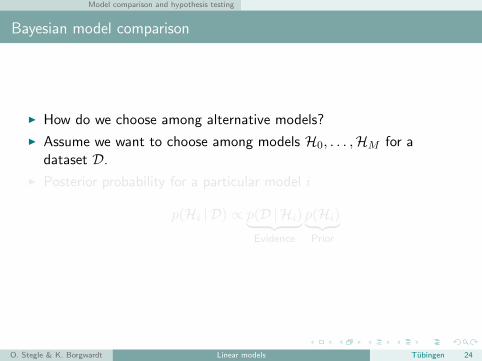
Model comparisonMotivation
I What degree of polynomialsdescribes the data best?
I Is the linear model at allappropriate?
I Association testing.
O. Stegle & K. Borgwardt Linear models Tubingen 23
Model comparison and hypothesis testing
Model comparisonMotivation
I What degree of polynomialsdescribes the data best?