On Explore-Then-Commit Strategies

Aurélien Garivier∗Institut de Mathématiques de Toulouse; UMR5219

Université de Toulouse; CNRSUPS IMT, F-31062 Toulouse Cedex 9, France

aurelien.garivier@math.univ-toulouse.fr

Emilie KaufmannUniv. Lille, CNRS, Centrale Lille, Inria SequeL

UMR 9189, CRIStAL - Centre de Recherche en Informatique Signal et Automatique de LilleF-59000 Lille, France

emilie.kaufmann@univ-lille1.fr

Tor LattimoreUniversity of Alberta

116 St & 85 Ave, Edmonton, AB T6G 2R3, Canadator.lattimore@gmail.com

Abstract

We study the problem of minimising regret in two-armed bandit problems withGaussian rewards. Our objective is to use this simple setting to illustrate thatstrategies based on an exploration phase (up to a stopping time) followed byexploitation are necessarily suboptimal. The results hold regardless of whetheror not the difference in means between the two arms is known. Besides themain message, we also refine existing deviation inequalities, which allow us todesign fully sequential strategies with finite-time regret guarantees that are (a)asymptotically optimal as the horizon grows and (b) order-optimal in the minimaxsense. Furthermore we provide empirical evidence that the theory also holds inpractice and discuss extensions to non-gaussian and multiple-armed case.

1 Introduction

It is now a very frequent issue for companies to optimise their daily profits by choosing betweenone of two possible website layouts. A natural approach is to start with a period of A/B Testing(exploration) during which the two versions are uniformly presented to users. Once the testing iscomplete, the company displays the version believed to generate the most profit for the rest of themonth (exploitation). The time spent exploring may be chosen adaptively based on past observations,but could also be fixed in advance. Our contribution is to show that strategies of this form aremuch worse than if the company is allowed to dynamically select which website to display withoutrestrictions for the whole month.

Our analysis focuses on a simple sequential decision problem played over T time-steps. In time-stept ∈ 1, 2, . . . , T the agent chooses an action At ∈ 1, 2 and receives a normally distributed reward

∗This work was partially supported by the CIMI (Centre International de Mathématiques et d’Informatique)Excellence program while Emilie Kaufmann visited Toulouse in November 2015. The authors acknowledge thesupport of the French Agence Nationale de la Recherche (ANR), under grants ANR-13-BS01-0005 (projectSPADRO) and ANR-13-CORD-0020 (project ALICIA).

30th Conference on Neural Information Processing Systems (NIPS 2016), Barcelona, Spain.

arX

iv:1

605.

0898

8v2

[m

ath.

ST]

14

Nov

201

6

Zt ∼ N (µAt , 1) where µ1, µ2 ∈ R are the unknown mean rewards for actions 1 and 2 respectively.The goal is to find a strategy π (a way of choosing each action At based on past observation) thatmaximises the cumulative reward over T steps in expectation, or equivalently minimises the regret

Rπµ(T ) = T max µ1, µ2 − Eµ

[T∑t=1

µAt

]. (1)

This framework is known as the multi-armed bandit problem, which has many applications andhas been studied for almost a century [Thompson, 1933]. Although this setting is now quite wellunderstood, the purpose of this article is to show that strategies based on distinct phases of explorationand exploitation are necessarily suboptimal. This is an important message because explorationfollowed by exploitation is the most natural approach and is often implemented in applications(including the website optimisation problem described above). Moreover, strategies of this kindhave been proposed in the literature for more complicated settings [Auer and Ortner, 2010, Perchetand Rigollet, 2013, Perchet et al., 2015]. Recent progress on optimal exploration policies (e.g., byGarivier and Kaufmann [2016]) could have suggested that well-tuned variants of two-phase strategiesmight be near-optimal. We show, on the contrary, that optimal strategies for multi-armed banditproblems must be fully-sequential, and in particular should mix exploration and exploitation. It isknown since the work of Wald [1945] on simple hypothese testing that sequential procedures can leadto significant gains. Here, the superiority of fully sequential procedures is consistent with intuition: ifone arm first appears to be better, but if subsequent observations are disappointing, the obligation tocommit at some point can be restrictive. In this paper, we give a crisp and precise description of howrestrictive it is: it leads to regret asympotically twice as large on average. The proof of this resultcombines some classical techniques of sequential analysis and of the bandit literature.

We study two settings, one when the gap ∆ = |µ1 − µ2| is known and the other when it is not.The most straight-forward strategy in the former case is to explore each action a fixed numberof times n and subsequently exploit by choosing the action that appeared best while exploring.It is easy to calculate the optimal n and consequently show that this strategy suffers a regret ofRπµ(T ) ∼ 4 log(T )/∆. A more general approach is to use a so-called Explore-Then-Commit (ETC)strategy, following a nomenclature introduced by Perchet et al. [2015]. An ETC strategy exploreseach action alternately until some data-dependent stopping time and subsequently commits to a singleaction for the remaining time-steps. We show in Theorem 2 that by using a sequential probability ratiotest (SPRT) it is possible to design an ETC strategy for which Rπµ(T ) ∼ log(T )/∆, which improveson the above result by a factor of 4. We also prove a lower bound showing that no ETC strategy canimprove on this result. Surprisingly it is possible to do even better by using a fully sequential strategyinspired by the UCB algorithm for multi-armed bandits [Katehakis and Robbins, 1995]. We design anew strategy for which Rπµ(T ) ∼ log(T )/(2∆), which improves on the fixed-design strategy by afactor of 8 and on SPRT by a factor of 2. Again we prove a lower bound showing that no strategy canimprove on this result.

For the case where ∆ is unknown, fixed-design strategies are hopeless because there is no reasonabletuning for the exploration budget n. However, it is possible to design an ETC strategy for unknowngaps. Our approach uses a modified fixed-budget best arm identification (BAI) algorithm in itsexploration phase (see e.g., Even-Dar et al. [2006], Garivier and Kaufmann [2016]) and chooses therecommended arm for the remaining time-steps. In Theorem 5 we show that a strategy based onthis idea satisfies Rπµ(T ) ∼ 4 log(T )/∆, which again we show is optimal within the class of ETCstrategies. As before, strategies based on ETC are suboptimal by a factor of 2 relative to the optimalrates achieved by fully sequential strategies such as UCB, which satisfies Rπµ(T ) ∼ 2 log(T )/∆[Katehakis and Robbins, 1995].

In a nutshell, strategies based on fixed-design or ETC are necessarily suboptimal. That this failureoccurs even in the simple setting considered here is a strong indicator that they are suboptimal inmore complicated settings. Our main contribution, presented in more details in Section 2, is to fullycharacterise the achievable asymptotic regret when ∆ is either known or unknown and the strategiesare either fixed-design, ETC or fully sequential. All upper bounds have explicit finite-time forms,which allow us to derive optimal minimax guarantees. For the lower bounds we give a novel andgeneric proof of all results. All proofs contain new, original ideas that we believe are fundamental tothe understanding of sequential analysis.

2

2 Notation and Summary of Results

We assume that the horizon T is known to the agent. The optimal action is a∗ = arg max(µ1, µ2), itsmean reward is µ∗ = µa∗ , and the gap between the means is ∆ = |µ1 − µ2|. LetH = R2 be the setof all possible pairs of means, andH∆ =

µ ∈ R2 : |µ1 − µ2| = ∆

. For i ∈ 1, 2 and n ∈ N let

µi,n be the empirical mean of the ith action based on the first n samples. Let At be the action chosenin time-step t and Ni(t) =

∑ts=1 1 As = i be the number of times the ith action has been chosen

after time-step t. We denote by µi(t) = µi,Ni(t) the empirical mean of the ith arm after time-step t.

A strategy is denoted by π, which is a function from past actions/rewards to a distribution over thenext actions. An ETC strategy is governed by a sampling rule (which determines which arm to sampleat each step), a stopping rule (which specifies when to stop the exploration phase) and a decisionrule indicating which arm is chosen in the exploitation phase. As we consider two-armed, Gaussianbandits with equal variances, we focus here on uniform sampling rules, which have been shownin Kaufmann et al. [2014] to be optimal in that setting. For this reason, we define an ETC strategy asa pair (τ, a), where τ is an even stopping time with respect to the filtration (Ft = σ(Z1, . . . , Zt))tand a ∈ 1, 2 is Fτ -measurable. In all the ETC strategies presented in this paper, the stopping timeτ depends on the horizon T (although this is not reflected in the notation). At time t, the action

picked by the ETC strategy is At =

1 if t ≤ τ and t is odd ,2 if t ≤ τ and t is even ,a otherwise .

The regret for strategy π, given in Eq. (1), depends on T and µ. Assuming, for example that µ1 =µ2 + ∆, then an ETC strategy π chooses the suboptimal arm N2(T ) = τ∧T

2 + (T − τ)+1 a = 2times, and the regret Rπµ(T ) = ∆Eµ[N2(T )] thus satisfies

∆Eµ[(τ ∧ T )/2] ≤ Rπµ(T ) ≤ (∆/2)Eµ[τ ∧ T ] + ∆T Pµ(τ ≤ T, a 6= a∗) . (2)

We denote the set of all ETC strategies by ΠETC. A fixed-design strategy is and ETC strategy forwhich there exists an integer n such that τ = 2n almost surely, and the set of all such strategies isdenoted by ΠDETC. The set of all strategies is denoted by ΠALL. For S ∈ H,H∆, we are interestedin strategies π that are uniformly efficient on S, in the sense that

∀µ ∈ S,∀α > 0, Rπµ(T ) = o(Tα). (3)

ΠALL ΠETC ΠDETC

H 2 4 NA

H∆ 1/2 1 4

We show in this paper that any uniformly efficient strategy in Πhas a regret at least equal to CΠ

S log(T )/|µ1 − µ2|(1− oT (1))for every parameter µ ∈ S , where CΠ

S is given in the adjacenttable. Furthermore, we prove that these results are tight. Ineach case, we propose a uniformly efficient strategy matchingthis bound. In addition, we prove a tight and non-asymptotic regret bound which also implies, inparticular, minimax rate-optimality.

The paper is organised as follows. First we consider ETC and fixed-design strategies when ∆ knownand unknown (Section 3). We then analyse fully sequential strategies that interleave exploration andexploitation in an optimal way (Section 4). For known ∆ we present a novel algorithm that exploitsthe additional information to improve the regret. For unknown ∆ we briefly recall the well-knownresults, but also propose a new regret analysis of the UCB* algorithm, a variant of UCB that canbe traced back to Lai [1987], for which we also obtain order-optimal minimax regret. Numericalexperiments illustrate and empirically support our results in Section 5. We conclude with a shortdiscussion on non-uniform exploration, and on models with more than 2 arms, possibly non Gaussian.All the proofs are given in the supplementary material. In particular, our simple, unified proof for allthe lower bounds is given in Appendix A.

3 Explore-Then-Commit Strategies

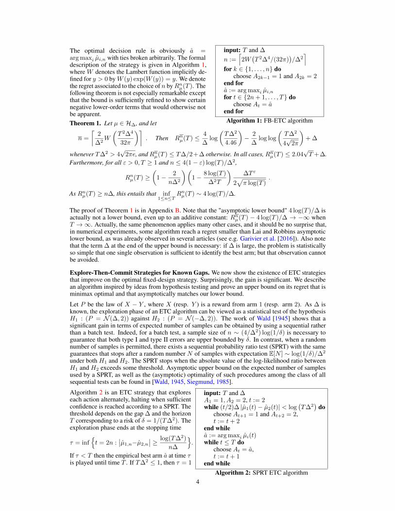
Fixed Design Strategies for Known Gaps. As a warm-up we start with the fixed-design ETCsetting where ∆ is known and where the agent chooses each action n times before committing for theremainder.

3

input: T and ∆

n :=⌈2W(T 2∆4/(32π)

)/∆2

⌉for k ∈ 1, . . . , n do

choose A2k−1 = 1 and A2k = 2end fora := arg maxi µi,nfor t ∈ 2n+ 1, . . . , T do

choose At = aend forAlgorithm 1: FB-ETC algorithm

The optimal decision rule is obviously a =arg maxi µi,n with ties broken arbitrarily. The formaldescription of the strategy is given in Algorithm 1,where W denotes the Lambert function implicitly de-fined for y > 0 by W (y) exp(W (y)) = y. We denotethe regret associated to the choice of n byRnµ(T ). Thefollowing theorem is not especially remarkable exceptthat the bound is sufficiently refined to show certainnegative lower-order terms that would otherwise notbe apparent.Theorem 1. Let µ ∈ H∆, and let

n =

⌈2

∆2W

(T 2∆4

32π

)⌉. Then Rnµ(T ) ≤ 4

∆log

(T∆2

4.46

)− 2

∆log log

(T∆2

4√

2π

)+ ∆

whenever T∆2 > 4√

2πe, andRnµ(T ) ≤ T∆/2+∆ otherwise. In all cases, Rnµ(T ) ≤ 2.04√T +∆.

Furthermore, for all ε > 0, T ≥ 1 and n ≤ 4(1− ε) log(T )/∆2,

Rnµ(T ) ≥(

1− 2

n∆2

)(1− 8 log(T )

∆2T

)∆T ε

2√π log(T )

.

As Rnµ(T ) ≥ n∆, this entails that inf1≤n≤T

Rnµ(T ) ∼ 4 log(T )/∆.

The proof of Theorem 1 is in Appendix B. Note that the "asymptotic lower bound" 4 log(T )/∆ isactually not a lower bound, even up to an additive constant: Rnµ(T ) − 4 log(T )/∆ → −∞ whenT →∞. Actually, the same phenomenon applies many other cases, and it should be no surprise that,in numerical experiments, some algorithm reach a regret smaller than Lai and Robbins asymptoticlower bound, as was already observed in several articles (see e.g. Garivier et al. [2016]). Also notethat the term ∆ at the end of the upper bound is necessary: if ∆ is large, the problem is statisticallyso simple that one single observation is sufficient to identify the best arm; but that observation cannotbe avoided.

Explore-Then-Commit Strategies for Known Gaps. We now show the existence of ETC strategiesthat improve on the optimal fixed-design strategy. Surprisingly, the gain is significant. We describean algorithm inspired by ideas from hypothesis testing and prove an upper bound on its regret that isminimax optimal and that asymptotically matches our lower bound.

Let P be the law of X − Y , where X (resp. Y ) is a reward from arm 1 (resp. arm 2). As ∆ isknown, the exploration phase of an ETC algorithm can be viewed as a statistical test of the hypothesisH1 : (P = N (∆, 2)) against H2 : (P = N (−∆, 2)). The work of Wald [1945] shows that asignificant gain in terms of expected number of samples can be obtained by using a sequential ratherthan a batch test. Indeed, for a batch test, a sample size of n ∼ (4/∆2) log(1/δ) is necessary toguarantee that both type I and type II errors are upper bounded by δ. In contrast, when a randomnumber of samples is permitted, there exists a sequential probability ratio test (SPRT) with the sameguarantees that stops after a random number N of samples with expectation E[N ] ∼ log(1/δ)/∆2

under both H1 and H2. The SPRT stops when the absolute value of the log-likelihood ratio betweenH1 and H2 exceeds some threshold. Asymptotic upper bound on the expected number of samplesused by a SPRT, as well as the (asymptotic) optimality of such procedures among the class of allsequential tests can be found in [Wald, 1945, Siegmund, 1985].

input: T and ∆A1 = 1, A2 = 2, t := 2while (t/2)∆ |µ1(t)− µ2(t)| < log

(T∆2

)do

choose At+1 = 1 and At+2 = 2,t := t+ 2

end whilea := arg maxi µi(t)while t ≤ T do

choose At = a,t := t+ 1

end whileAlgorithm 2: SPRT ETC algorithm

Algorithm 2 is an ETC strategy that exploreseach action alternately, halting when sufficientconfidence is reached according to a SPRT. Thethreshold depends on the gap ∆ and the horizonT corresponding to a risk of δ = 1/(T∆2). Theexploration phase ends at the stopping time

τ = inft = 2n :

∣∣µ1,n−µ2,n

∣∣ ≥ log(T∆2)

n∆

.

If τ < T then the empirical best arm a at time τis played until time T . If T∆2 ≤ 1, then τ = 1

4

(one could even define τ = 0 and pick a random arm). The following theorem gives a non-asymptoticupper bound on the regret of the algorithm. The results rely on non-asymptotic upper bounds on theexpectation of τ , which are interesting in their own right.Theorem 2. If T∆2 ≥ 1, then the regret of the SPRT-ETC algorithm is upper-bounded as

RSPRT-ETCµ (T ) ≤ log(eT∆2)

∆+

4√

log(T∆2) + 4

∆+ ∆ .

Otherwise it is upper bounded by T∆/2+∆, and for all T and ∆ the regret is less than 10√T/e+∆.

The proof of Theorem 2 is given in Appendix C. The following lower bound shows that no uniformlyefficient ETC strategy can improve on the asymptotic regret of Algorithm 2. The proof is given inSection A together with the other lower bounds.Theorem 3. Let π be an ETC strategy that is uniformly efficient onH∆. Then for all µ ∈ H∆,

lim infT→∞

Rπµ(T )

log(T )≥ 1

∆.

Explore-Then-Commit Strategies for Unknown Gaps. When the gap is unknown it is not possibleto tune a fixed-design strategy that achieves logarithmic regret. ETC strategies can enjoy logarithmicregret and these are now analysed. We start with the asymptotic lower bound.Theorem 4. Let π be a uniformly efficient ETC strategy onH. For all µ ∈ H, if ∆ = |µ1 − µ2| then

lim infT→∞

Rπµ(T )

log(T )≥ 4

∆.

A simple idea for constructing an algorithm that matches the lower bound is to use a (fixed-confidence)best arm identification algorithm for the exploration phase. Given a risk parameter δ, a δ-PAC BAIalgorithm consists of a sampling rule (At), a stopping rule τ and a recommendation rule a whichis Fτ measurable and satisfies, for all µ ∈ H such that µ1 6= µ2, Pµ(a = a∗) ≥ 1− δ. In a banditmodel with two Gaussian arms, Kaufmann et al. [2014] propose a δ-PAC algorithm using a uniformsampling rule and a stopping rule τδ that asymptotically attains the minimal sample complexityEµ[τδ] ∼ (8/∆2) log(1/δ). Using the regret decomposition (2), it is easy to show that the ETCalgorithm using the stopping rule τδ for δ = 1/T matches the lower bound of Theorem 4.

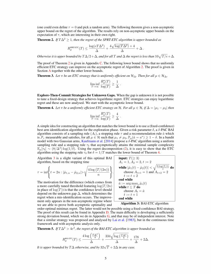
input: T (≥ 3)A1 = 1, A2 = 2, t := 2

while |µ1(t)− µ2(t)| <√

8 log(T/t)t do

choose At+1 = 1 and At+2 = 2t := t+ 2

end whilea := arg maxi µi(t)while t ≤ T do

choose At = at := t+ 1

end whileAlgorithm 3: BAI-ETC algorithm

Algorithm 3 is a slight variant of this optimal BAIalgorithm, based on the stopping time

τ = inf

t = 2n : |µ1,n − µ2,n|>

√4 log

(T/(2n)

)n

.The motivation for the difference (which comes froma more carefully tuned threshold featuring log(T/2n)in place of log(T )) is that the confidence level shoulddepend on the unknown gap ∆, which determines theregret when a mis-identification occurs. The improve-ment only appears in the non-asymptotic regime wherewe are able to prove both asymptotic optimality andorder-optimal minimax regret. The latter would not be possible using a fixed-confidence BAI strategy.The proof of this result can be found in Appendix D. The main difficulty is developing a sufficientlystrong deviation bound, which we do in Appendix G, and that may be of independent interest. Notethat a similar strategy was proposed and analysed by Lai et al. [1983], but in the continuous timeframework and with asymptotic analysis only.Theorem 5. If T∆2 > 4e2, the regret of the BAI-ETC algorithm is upper bounded as

RBAI-ETCµ (T ) ≤

4 log(T∆2

4

)∆

+334√

log(T∆2

4

)∆

+178

∆+ 2∆.

It is upper bounded by T∆ otherwise, and by 32√T + 2∆ in any case.

5

4 Fully Sequential Strategies for Known and Unknown Gaps

In the previous section we saw that allowing a random stopping time leads to a factor of 4 improvementin terms of the asymptotic regret relative to the naive fixed-design strategy. We now turn our attentionto fully sequential strategies when ∆ is known and unknown. The latter case is the classic 2-armedbandit problem and is now quite well understood. Our modest contribution in that case is the firstalgorithm that is simultaneously asymptotically optimal and order optimal in the minimax sense. Forthe former case, we are not aware of any previous research where the gap is known except the line ofwork by Bubeck et al. [2013], Bubeck and Liu [2013], where different questions are treated. In bothcases we see that fully sequential strategies improve on the best ETC strategies by a factor of 2.

Known Gaps. We start by stating the lower bound (proved in Section A), which is a straightforwardgeneralisation of Lai and Robbins’ lower bound.Theorem 6. Let π be a strategy that is uniformly efficient onH∆. Then for all µ ∈ H∆,

lim infT→∞

Rπµ(T )

log T≥ 1

2∆

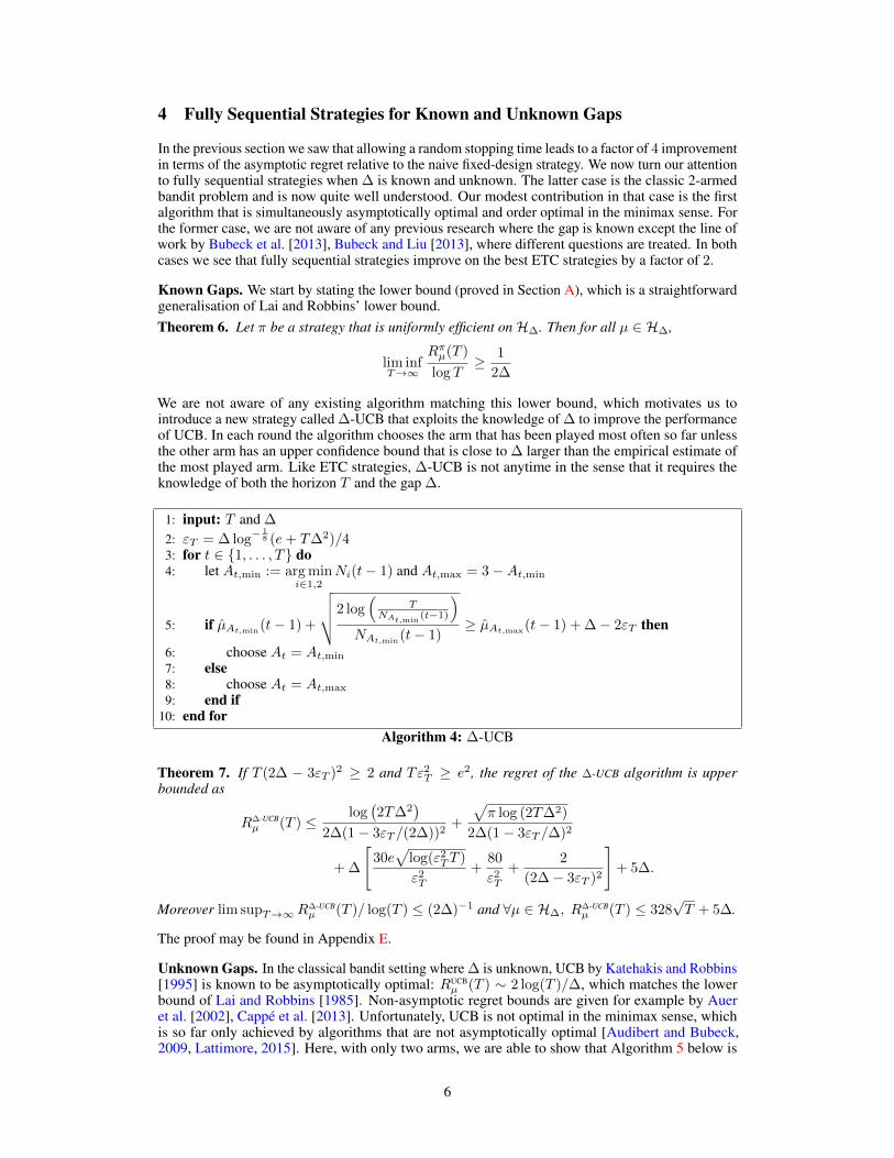
We are not aware of any existing algorithm matching this lower bound, which motivates us tointroduce a new strategy called ∆-UCB that exploits the knowledge of ∆ to improve the performanceof UCB. In each round the algorithm chooses the arm that has been played most often so far unlessthe other arm has an upper confidence bound that is close to ∆ larger than the empirical estimate ofthe most played arm. Like ETC strategies, ∆-UCB is not anytime in the sense that it requires theknowledge of both the horizon T and the gap ∆.

1: input: T and ∆

2: εT = ∆ log−18 (e+ T∆2)/4

3: for t ∈ 1, . . . , T do4: let At,min := arg min

i∈1,2Ni(t− 1) and At,max = 3−At,min

5: if µAt,min(t− 1) +

√√√√2 log(

TNAt,min

(t−1)

)NAt,min

(t− 1)≥ µAt,max

(t− 1) + ∆− 2εT then

6: choose At = At,min

7: else8: choose At = At,max

9: end if10: end for

Algorithm 4: ∆-UCB

Theorem 7. If T (2∆ − 3εT )2 ≥ 2 and Tε2T ≥ e2, the regret of the ∆-UCB algorithm is upper

bounded as

R∆-UCBµ (T ) ≤

log(2T∆2

)2∆(1− 3εT /(2∆))2

+

√π log (2T∆2)

2∆(1− 3εT /∆)2

+ ∆

[30e√

log(ε2TT )

ε2T

+80

ε2T

+2

(2∆− 3εT )2

]+ 5∆.

Moreover lim supT→∞R∆-UCBµ (T )/ log(T ) ≤ (2∆)−1 and ∀µ ∈ H∆, R

∆-UCBµ (T ) ≤ 328

√T + 5∆.

The proof may be found in Appendix E.

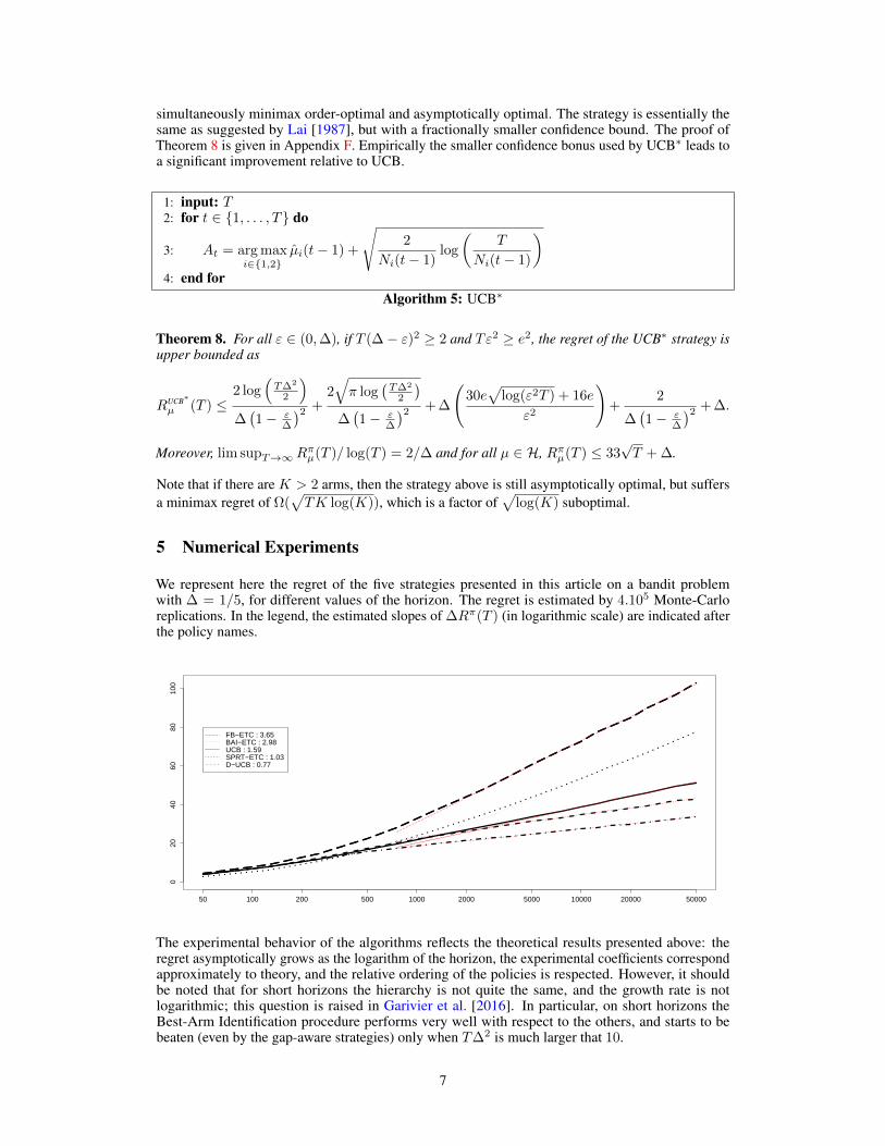
Unknown Gaps. In the classical bandit setting where ∆ is unknown, UCB by Katehakis and Robbins[1995] is known to be asymptotically optimal: RUCB

µ (T ) ∼ 2 log(T )/∆, which matches the lowerbound of Lai and Robbins [1985]. Non-asymptotic regret bounds are given for example by Aueret al. [2002], Cappé et al. [2013]. Unfortunately, UCB is not optimal in the minimax sense, whichis so far only achieved by algorithms that are not asymptotically optimal [Audibert and Bubeck,2009, Lattimore, 2015]. Here, with only two arms, we are able to show that Algorithm 5 below is

6

simultaneously minimax order-optimal and asymptotically optimal. The strategy is essentially thesame as suggested by Lai [1987], but with a fractionally smaller confidence bound. The proof ofTheorem 8 is given in Appendix F. Empirically the smaller confidence bonus used by UCB∗ leads toa significant improvement relative to UCB.

1: input: T2: for t ∈ 1, . . . , T do

3: At = arg maxi∈1,2

µi(t− 1) +

√2

Ni(t− 1)log

(T

Ni(t− 1)

)4: end for

Algorithm 5: UCB∗

Theorem 8. For all ε ∈ (0,∆), if T (∆− ε)2 ≥ 2 and Tε2 ≥ e2, the regret of the UCB∗ strategy isupper bounded as

RUCB∗

µ (T ) ≤2 log

(T∆2

2

)∆(1− ε

∆

)2 +2√π log

(T∆2

2

)∆(1− ε

∆

)2 + ∆

(30e√

log(ε2T ) + 16e

ε2

)+

2

∆(1− ε

∆

)2 + ∆.

Moreover, lim supT→∞Rπµ(T )/ log(T ) = 2/∆ and for all µ ∈ H, Rπµ(T ) ≤ 33√T + ∆.

Note that if there are K > 2 arms, then the strategy above is still asymptotically optimal, but suffersa minimax regret of Ω(

√TK log(K)), which is a factor of

√log(K) suboptimal.

5 Numerical Experiments

We represent here the regret of the five strategies presented in this article on a bandit problemwith ∆ = 1/5, for different values of the horizon. The regret is estimated by 4.105 Monte-Carloreplications. In the legend, the estimated slopes of ∆Rπ(T ) (in logarithmic scale) are indicated afterthe policy names.

50 100 200 500 1000 2000 5000 10000 20000 50000

020

4060

8010

0

FB−ETC : 3.65BAI−ETC : 2.98UCB : 1.59SPRT−ETC : 1.03D−UCB : 0.77

The experimental behavior of the algorithms reflects the theoretical results presented above: theregret asymptotically grows as the logarithm of the horizon, the experimental coefficients correspondapproximately to theory, and the relative ordering of the policies is respected. However, it shouldbe noted that for short horizons the hierarchy is not quite the same, and the growth rate is notlogarithmic; this question is raised in Garivier et al. [2016]. In particular, on short horizons theBest-Arm Identification procedure performs very well with respect to the others, and starts to bebeaten (even by the gap-aware strategies) only when T∆2 is much larger that 10.

7

6 Conclusion: Beyond Uniform Exploration, Two Arms and Gaussiandistributions

It is worth emphasising the impossibility of non-trivial lower bounds on the regret of ETC strategiesusing any possible (non-uniform) sampling rule. Indeed, using UCB as a sampling rule together withan a.s. infinite stopping rule defines an artificial but formally valid ETC strategy that achieves the bestpossible rate for general strategies. This strategy is not a faithful counter-example to our claim thatETC strategies are sub-optimal, because UCB is not a satisfying exploration rule. If exploration is theobjective, then uniform sampling is known to be optimal in the two-armed Gaussian case [Kaufmannet al., 2014], which justifies the uniform sampling assumption.

The use of ETC strategies for regret minimisation (e.g., as presented by Perchet and Rigollet [2013])is certainly not limited to bandit models with 2 arms. The extension to multiple arms is based on thesuccessive elimination idea in which a set of active arms is maintained with arms chosen accordingto a round robin within the active set. Arms are eliminated from the active set once their optimalitybecomes implausible and the exploration phase terminates when the active set contains only a singlearm (an example is by Auer and Ortner [2010]). The Successive Elimination algorithm has beenintroduced by Even-Dar et al. [2006] for best-arm identification in the fixed-confidence setting. It wasshown to be rate-optimal, and thus a good compromise for both minimizing regret and finding thebest arm. If one looks more precisely at mutliplicative constants, however, Garivier and Kaufmann[2016] showed that it is suboptimal for the best arm identification task in almost all settings excepttwo-armed Gaussian bandits. Regarding regret minimization, the present paper shows that it issub-optimal by a factor 2 on every two-armed Gaussian problem.

It is therefore interesting to investigate the performance in terms of regret of an ETC algorithmusing an optimal BAI algorithm. This is actually possible not only for Gaussian distributions, butmore generally for one-parameter exponential families, for which Garivier and Kaufmann [2016]propose the asymptotically optimal Track-and-Stop strategy. Denoting d(µ, µ′) = KL(νµ, νµ′) theKullback-Leibler divergence between two distributions parameterised by µ and µ′, they provideresults which can be adapted to obtain the following bound.Proposition 1. For µ such that µ1 > maxa6=1 µa, the regret of the ETC strategy using Track-and-Stopexploration with risk 1/T satisfies

lim supT→∞

RTaSµ (T )

log T≤ T ∗(µ)

(K∑a=2

w∗a(µ)(µ1 − µa)

),

where T ∗(µ) (resp. w∗(µ)) is the the maximum (resp. maximiser) of the optimisation problem

maxw∈ΣK

infa6=1

[w1d

(µ1,

w1µ1 + waµaw1 + wa

)+ wad

(µa,

waµ1 + waµaw1 + wa

)],

where ΣK is the set of probability distributions on 1, . . . ,K.

In general, it is not easy to quantify the difference to the lower bound of Lai and Robbins

lim infT→∞

Rπµ(T )

log T≥

K∑a=2

µ1 − µad(µa, µ1)

.

Even for Gaussian distributions, there is no general closed-form formula for T ∗(µ) and w∗(µ) exceptwhen K = 2. However, we conjecture that the worst case is when µ1 and µ2 are much larger thanthe other means: then, the regret is almost the same as in the 2-arm case, and ETC strategies aresuboptimal by a factor 2. On the other hand, the most favourable case (in terms of relative efficiency)seems to be when µ2 = · · · = µK : then

w∗1(µ) =

√K − 1

K − 1 +√K − 1

, w∗2(µ) = · · · = w∗K(µ) =1

K − 1 +√K − 1

and T ∗ = 2(√K − 1 + 1)2/∆2, leading to

lim supT→∞

RTaSµ (T )

log(T )≤(

1 +1√

K − 1

)2(K − 1)

∆,

while Lai and Robbins’ lower bound yields 2(K − 1)/∆. Thus, the difference grows with K as2√K − 1 log(T )/∆ , but the relative difference decreases.

8

ReferencesJean-Yves Audibert and Sébastien Bubeck. Minimax policies for adversarial and stochastic bandits.

In Proceedings of Conference on Learning Theory (COLT), pages 217–226, 2009.

Peter Auer and Ronald Ortner. UCB revisited: Improved regret bounds for the stochastic multi-armedbandit problem. Periodica Mathematica Hungarica, 61(1-2):55–65, 2010.

Peter Auer, Nicoló Cesa-Bianchi, and Paul Fischer. Finite-time analysis of the multiarmed banditproblem. Machine Learning, 47:235–256, 2002.

Sébastien Bubeck and Che-Yu Liu. Prior-free and prior-dependent regret bounds for thompsonsampling. In Advances in Neural Information Processing Systems, pages 638–646, 2013.

Sébastien Bubeck, Vianney Perchet, and Philippe Rigollet. Bounded regret in stochastic multi-armedbandits. In Proceedings of the 26th Conference On Learning Theory, pages 122–134, 2013.

Olivier Cappé, Aurélien Garivier, Odalric-Ambrym Maillard, Rémi Munos, and Gilles Stoltz.Kullback–Leibler upper confidence bounds for optimal sequential allocation. The Annals ofStatistics, 41(3):1516–1541, 2013.

Eyal Even-Dar, Shie Mannor, and Yishay Mansour. Action Elimination and Stopping Conditions forthe Multi-Armed Bandit and Reinforcement Learning Problems. Journal of Machine LearningResearch, 7:1079–1105, 2006.

Aurélien Garivier and Emilie Kaufmann. Optimal best arm identification with fixed confidence. InProceedings of the 29th Conference On Learning Theory (to appear), 2016.

Aurélien Garivier, Pierre Ménard, and Gilles Stoltz. Explore first, exploit next: The true shape ofregret in bandit problems. arXiv preprint arXiv:1602.07182, 2016.

Abdolhossein Hoorfar and Mehdi Hassani. Inequalities on the lambert w function and hyperpowerfunction. J. Inequal. Pure and Appl. Math, 9(2):5–9, 2008.

Michael N Katehakis and Herbert Robbins. Sequential choice from several populations. Proceedingsof the National Academy of Sciences of the United States of America, 92(19):8584, 1995.

Emilie Kaufmann, Olivier Cappé, and Aurélien Garivier. On the Complexity of A/B Testing. InProceedings of the 27th Conference On Learning Theory, 2014.

Tze Leung Lai. Adaptive treatment allocation and the multi-armed bandit problem. The Annals ofStatistics, pages 1091–1114, 1987.

Tze Leung Lai and Herbert Robbins. Asymptotically efficient adaptive allocation rules. Advances inapplied mathematics, 6(1):4–22, 1985.

Tze Leung Lai, Herbert Robbins, and David Siegmund. Sequential design of comparative clinicaltrials. In M. Haseeb Rizvi, Jagdish Rustagi, and David Siegmund, editors, Recent advances instatistics: papers in honor of Herman Chernoff on his sixtieth birthday, pages 51–68. AcademicPress, 1983.

Tor Lattimore. Optimally confident UCB: Improved regret for finite-armed bandits. Technical report,2015. URL http://arxiv.org/abs/1507.07880.

Peter Mörters and Yuval Peres. Brownian motion, volume 30. Cambridge University Press, 2010.

Vianney Perchet and Philippe Rigollet. The multi-armed bandit with covariates. The Annals ofStatistics, 2013.

Vianney Perchet, Philippe Rigollet, Sylvain Chassang, and Eric Snowberg. Batched bandit problems.In Proceedings of the 28th Conference On Learning Theory, 2015.

David Siegmund. Sequential Analysis. Springer-Verlag, 1985.

William Thompson. On the likelihood that one unknown probability exceeds another in view of theevidence of two samples. Biometrika, 25(3/4):285–294, 1933.

Abraham Wald. Sequential Tests of Statistical Hypotheses. Annals of Mathematical Statistics, 16(2):117–186, 1945.

9

Notation for the Proofs

We denote by (Xs) and (Ys) the sequence of successive observations from arm 1 and arm 2, so that

µ1,s =1

s

s∑i=1

Xi and µ2,s =1

s

s∑i=1

Yi

In the proofs of all regret upper bounds given in Appendix B to F we assume without loss of generalitythat µ is such that µ1 > µ2 and let ∆ = µ1 − µ2.

A Proof of the Lower Bounds (Theorems 3, 4, 6 and Lai&Robbins)

Let π be a uniformly efficient strategy on some class S, as defined in (3), and let λ ∈ H. Ifm(λ) = arg minλ1, λ2, as Eλ[Rπµ(T )] = |λ1 − λ2|Eλ[Nm(λ)(T )] this implies in particular that

∀α ∈]0, 1], Eλ[Nm(λ)(T )] = o(Tα).

Without loss of generality we assume that µ1 = µ2 + ∆ with ∆ > 0. All the lower bounds are basedon a change of measure argument, which involves considering an alternative reward vector (µ′1, µ

′2)

that is “not too far” from (µ1, µ2), but for which the expected behaviour of the algorithm is verydifferent. This is the same approach used by Lai and Robbins [1985], but rewritten and generalised ina more powerful way (in particular regarding the ETC strategies). The improvements come thanks toInequality 4 in [Garivier et al., 2016], which states that for every (µ′1, µ

′2) ∈ H and for every stopping

time σ such that N2(T ) is Fσ-measurable,

Eµ[N1(σ)

] (µ′1 − µ1)2

2+ Eµ

[N2(σ)

] (µ′2 − µ2)2

2≥ kl

(Eµ[N2(T )

T

], Eµ′

[N2(T )

T

]),

where kl(p, q) is the relative entropy between Bernoulli distributions with parameters p, q ∈ [0, 1]respectively. Since kl(p, q) ≥ (1− p) log(1/(1− q))− log(2) for all p, q ∈ (0, 1), one obtains

Eµ[N1(σ)

] (µ′1 − µ1)2

2+ Eµ

[N2(σ)

] (µ′2 − µ2)2

2

≥(

1− Eµ[N2(T )]

T

)log

(T

Eµ′ [N1(T )]

)− log(2) . (4)

For µ′ ∈ S such that µ′1 < µ′2, Eµ[N2(T )] = o(Tα) and Eµ′ [N1(T )] = o(Tα) for all α ∈]0, 1], thus

lim infT→∞

Eµ[N1(σ)

](µ′1 − µ1)2/2 + Eµ

[N2(σ)

](µ′2 − µ2)2/2

log T≥ 1 .

Let us now draw the conclusions in each setting. Observe that while this argument is now routine forgeneral policies, we show here how to apply it very nicely to ETC strategies as well.

Known gap, General strategy: S = H∆. By choos-ing σ = T , µ′1 = µ1 and µ′2 = µ1 + ∆ = µ2 + 2∆,we obtain

lim infT→∞

Eµ[N2(T )

]log T

≥ 1

(2∆)2/2.

Unknown gap, General strategy:S = H. We use the same choices, ex-cept µ′2 = µ1 + ε for some ε > 0:

lim infT→∞

Eµ[N2(T )

]log T

≥ 1

(∆ + ε)2/2

.

Known gap, ETC strategy: S = H∆. For an ETCstrategy π with a stopping rule τ , one hasN1(τ∧T ) =N2(τ ∧ T ) = (τ ∧ T )/2. Besides, N2(T ) is indeedFτ∧T -measurable: after τ ∧T draws, the agent knowswhether she will draw arm 2 for the last T − τ ∧ Tsteps or not. With µ′1 = µ2, µ′2 = µ1, Inequality (4)thus yields:

lim infT→∞

Eµ[τ∧T

2

]log T

≥ 1

2∆2/2.

Unknown gap, ETC strategy: S = H.Choosing this time µ′1 = (µ1 + µ2 −ε)/2 and µ′2 = (µ1 + µ2 + ε)/2, forsome ε > 0 yields

lim infT→∞

Eµ[τ∧T

2

]log T

≥ 1(∆+ε

2

)2 .

10

Rπµ(T ) = ∆Eµ[N2(T )] for general strategies, while Equation (2) shows that Rπµ(T ) ≥ ∆Eµ[(τ ∧T )/2] for ETC strategies. Therefore letting ε go to zero when needed shows that

lim infT→∞

Rπµ(T )

log(T )≥ CΠ

S∆

, for the value CΠS given at the end of Section 2.

Note that the asymptotic lower bound of Theorem 1 can also be proved by similar arguments, if onereally wants to bring in an elephant to kill a mouse. Moreover, note that this proof may also lead to(not-so-simple) non-asymptotic lower-bounds, as shown in Garivier et al. [2016] for example.

B Proof of Theorem 1

Let n ≤ T/2. The number of draws of the suboptimal arm 2 is N2 = n + (T − 2n)1Sn ≤ 0,where Sn = (X1 − Y1) + · · ·+ (Xn − Yn) ∼ N (n∆, 2n). The expected regret of the strategy using2n exploration steps is

Rnµ(T ) = ∆Eµ[N2] = ∆(n+ (T − 2n)Pµ(Sn ≤ 0)

). (5)

But

Pµ(Sn ≤ 0) = Pµ(Sn − n∆√

2n≤ −n∆√

2n= −∆

√n

2

).

Denote by Φ (resp. φ) the pdf (resp. cdf) of the standard Gaussian distribution, and recall thatW is theLambert function defined for all y > 0 by W (y) exp(W (y)) = y. The regret is thus upper-boundedas Rnµ(T ) ≤ ∆g(n) where, for all x > 0, g(x) = x+ TΦ(−∆

√x/2). By differentiating g, one can

see that its maximum is reached at x∗ such that

φ

(∆

√x∗

2

)=

∆√x∗/2

T∆2/4, and thus x∗ =

2

∆2W

(T 2∆4

32π

).

By choosing n = dx∗e, we obtain

Rnµ(T ) ≤ 2

∆W

(T 2∆4

32π

)+ ∆ + ∆TΦ

(−∆

√x∗

2

).

As g(n) ≤ g(x∗) + 1 ≤ g(0) + 1 = T/2 + 1, Rnµ(T ) ≤ (T/2 + 1)∆ ≤ 2.04√T + ∆ for

T∆2 ≤ 4√

2πe. If T∆2 ≥ 4√

2πe, the inequality W (y) ≤ log((1 + e−1)y/ log(y)

)valid for all

y ≥ e (see Hoorfar and Hassani [2008]) entails

W

(T 2∆4

32π

)≤ log

((1 + e−1)T

2∆4

32π

log(T 2∆4

32π

) )= 2 log

1

8

√1 + e−1

π

T∆2√log(T∆2

4√

2π

)

In addition, the classic bound on the Gaussian tail Φ(−y) ≤ φ(y)/y yields by definition of x∗:

Φ

(−∆

√x∗

2

)≤φ(−∆

√x∗

2

)∆√

x∗

2

=4

T∆2.

Hence, for T∆2 ≥ 4√

2πe,

Rnµ(T ) ≤ 4

∆log

e

8

√1 + e−1

π

T∆2√log(T∆2

4√

2π

)+ ∆ <

4

∆log

T∆2

4.46

√log(T∆2

4√

2π

)+ ∆ .

To complete the proof of the uniform upper-bound, we start from

Rnµ(T ) ≤ 2

∆W

(T 2∆4

32π

)+

4

∆+ ∆ .

11

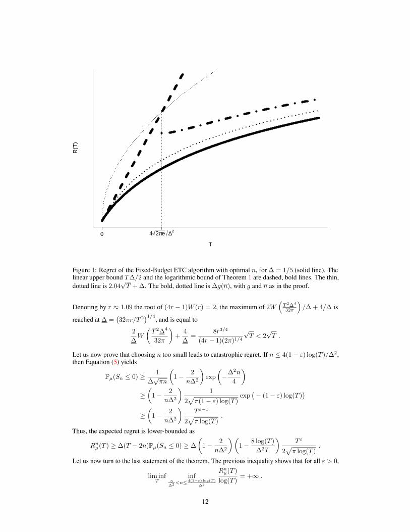
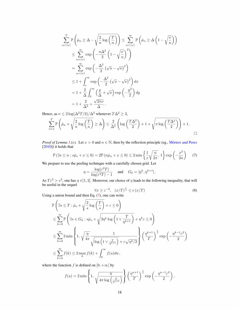
0 4 2πe ∆2

T

R(T

)

Figure 1: Regret of the Fixed-Budget ETC algorithm with optimal n, for ∆ = 1/5 (solid line). Thelinear upper bound T∆/2 and the logarithmic bound of Theorem 1 are dashed, bold lines. The thin,dotted line is 2.04

√T + ∆. The bold, dotted line is ∆g(n), with g and n as in the proof.

Denoting by r ≈ 1.09 the root of (4r − 1)W (r) = 2, the maximum of 2W(T 2∆4

32π

)/∆ + 4/∆ is

reached at ∆ =(32πr/T 2

)1/4, and is equal to

2

∆W

(T 2∆4

32π

)+

4

∆=

8r3/4

(4r − 1)(2π)1/4

√T < 2

√T .

Let us now prove that choosing n too small leads to catastrophic regret. If n ≤ 4(1− ε) log(T )/∆2,then Equation (5) yields

Pµ(Sn ≤ 0) ≥ 1

∆√πn

(1− 2

n∆2

)exp

(−∆2n

4

)≥(

1− 2

n∆2

)1

2√π(1− ε) log(T )

exp(− (1− ε) log(T )

)≥(

1− 2

n∆2

)T ε−1

2√π log(T )

.

Thus, the expected regret is lower-bounded as

Rnµ(T ) ≥ ∆(T − 2n)Pµ(Sn ≤ 0) ≥ ∆

(1− 2

n∆2

)(1− 8 log(T )

∆2T

)T ε

2√π log(T )

.

Let us now turn to the last statement of the theorem. The previous inequality shows that for all ε > 0,

lim infT

inf3

∆2<n≤4(1−ε) log(T )

∆2

Rnµ(T )

log(T )= +∞ .

12

For n ≤ 3/∆2, we have that

Pµ(Sn ≤ 0) ≥ Pµ

(Sn − n∆√

2n≤ −

√3

2

)> 0 ,

and hence that lim infT infn≤3/∆2 Rnµ(T )/T > 0. As Rnµ(T ) ≥ n∆, the result follows.

C Proof of Theorem 2

Recall that µ1 > µ2. Using (2), one has

Rπµ(T ) ≤ ∆Eµ[τ

2

]+ T∆Pµ(τ < T, a = 2) .

If T∆2 ≤ 1, then τ = 2 and a is based on a single sample from each action. Therefore a = 2 withprobability less than 1/2 and the regret is upper-bounded by ∆ + T∆/2. Otherwise, let S0 = 0,Sn = (X1−Y1)+ · · ·+(Xn−Yn) for every n ≥ 1. For every u > 0, let nu = (log(T∆2)+u)/∆2.Observe that τ

2≥⌈

log(T∆2) + u

∆2

⌉⊂Sdnue ≤

log(T∆2)

∆

.

Moreover, if nu ∈ N then Snu ∼ N (nu∆, 2nu) and

Pµ(Snu ≤

log(T∆2)

∆

)= Pµ

(Snu − nu∆√

2nu≤ log(T∆2)/∆−∆(log(T∆2) + u)/∆2√

2(log(T∆2) + u)/∆2

)

= Pµ

(Snu − nu∆√

2nu≤ −u√

2(log(T∆2) + u)

)≤ exp

(− u2

4(

log(T∆2) + u)) .

Hence, for a = 2√

log(T∆2),∫ ∞na

Pµ(τ

2− 1 ≥ v

)dv =

∫ ∞a

Pµ(τ

2− 1 ≥ log(T∆2) + u

∆2

)du

∆2

≤∫ ∞a

Pµ(τ

2≥⌈

log(T∆2) + u

∆2

)⌉du

∆2

≤ 1

∆2

∫ ∞a

exp

(− u2

4(

log(T∆2) + u)) du

≤ 1

∆2

∫ ∞a

exp

(− u

2√

log(T∆2) + 4

)du as log(T∆2) ≤ u

√log(∆2T )/2

≤ 1

∆2

∫ ∞0

exp

(− u

2√

log(T∆2) + 4

)du

=2√

log(T∆2) + 4

∆2,

and

Eµ[τ

2

]≤ 1 + na +

∫ ∞na

Pµ(τ

2− 1 ≥ v

)dv ≤ 1 +

log(T∆2) + 4√

log(T∆2) + 4

∆2.

To conclude the proof of the first statement, it remains to show that P(τ < T, a = 2) ≤ 1/(T∆2).Since X1 − Y1 ∼ N (∆, 2), Eµ[exp(−∆(X1 − Y1))] = exp(−∆2 + 2∆2/2) = 1 and Mn =exp(−∆Sn) is a martingale. Let τ2 = T ∧ infn ≥ 1 : Sn ≤ − log(T∆2)/∆, and observe that

τ < T, a = 2⊂∃n < T : Sn ≤ −

log(T∆2)

∆

=τ2 < T

.

13

Doob’s optional stopping theorem yields Eµ[Mτ2 ] = Eµ[M0] = 1. But as Mτ2 = exp(−∆Sτ2) ≥exp(∆ log(T∆2)/∆) = T∆2 on the event τ2 < T,

Pµ(τ < T, a = 2) ≤ Pµ(τ2 < T ) ≤ Eµ[1τ2 < TMτ2

T∆2

]≤

Eµ[Mτ2

]T∆2

=1

T∆2.

The last statement Theorem 2 is obtained by maximising the bound (except for the ∆ summand). Letu = 1/(∆

√T ) and f(u) = −u log(u/

√e) + 2u

√− log(u). Denoting ` = − log(u), f ′(u) = `−

1/2+2√`−1/

√` = (

√`+2)(`−1/2)/

√`, thus the maximum is reached at ` = log

(∆√T)

= 1/2

and ∆ =√e/T . Re-injecting this value into the bound, we obtain that for every ∆ > 0,

RSPRT-ETCµ (T ) ≤ 2 + 4

√1 + 4√

e/T= 10

√T

e.

D Proof of Theorem 5

Recall that µ1 = µ2 + ∆ with ∆ > 0. Let Ws = (Xs−Ys−∆)/√

2, which means that W1,W2, . . .are i.i.d. standard Gaussian random variables. Introducing F = (a 6= 1, τ < T ), one has by (2) that

RBAI-ETCµ (T ) ≤ T∆Pµ(F) + (∆/2)Eµ[τ ∧ T ].

From the definition of τ and Lemma 1.(c) in Appendix G, assuming that T∆2 ≥ 4e2, one obtains

Pµ (F) ≤ Pµ

(∃s : 2s ≤ T, µ1,s − µ2,s ≤ −

√4

slog

(T

2s

))

= Pµ

(∃s ≤ T/2 :

∑si=1Wi

s≤ −

√2

slog

(T/2

s

)− ∆√

2

)

≤120e

√log(∆2T/4)

∆2T+

64e

∆2T.

The last step is bounding Eµ[τ ∧ T ] for which as T∆2 ≥ 4, Lemma 1.(b) yields

Eµ[τ ∧ T ] =

T∑t=1

Pµ (τ ≥ t) ≤ 2 + 2

T/2∑s=1

Pµ (τ ≥ 2s+ 1)

≤ 2 + 2

T/2∑s=1

Pµ

(∑si=1Wi

s≤

√2

slog

(T/2

s

)− ∆√

2

)

≤8 log

(T∆2

4

)∆2

+8√π log

(T∆2

4

)∆2

+8

∆2+ 4 ,

Therefore, if T∆2 ≥ 4e2,

RBAI-ETCµ (T ) ≤

4 log(T∆2

4

)∆

+4√π log

(T∆2

4

)∆

+4

∆+ 2∆ +

120e√

log(

∆2T4

)∆

+64e

∆

≤4 log

(T∆2

4

)∆

+334√

log(T∆2

4

)∆

+178

∆+ 2∆.

Taking the limit as T → ∞ shows that lim supT→∞RBAI-ETCµ (T )/ log(T ) ≤ 4. Noting that

RBAI-ETCµ (T ) ≤ ∆T and taking the minimum of this bound and the finite-time bound given above

leads arduously to RBAI-ETCµ (T ) ≤ 2∆ + 32

√T for all µ.

14

E Proof of Theorem 7

Define random time τ = max τ1, τ2 where τi is given by

τi = min

t ≤ T : sup

s≥t|µi,s − µi| < εT

.

By the concentration Lemma 1.(a) in Appendix G we have Eµ[τi] ≤ 1 + 9/ε2T and so Eµ[τ ] ≤

Eµ[τ1 + τ2] ≤ 2 + 18/ε2T . For t > 2τ we have |µAt,max

(t − 1) − µAt,max| < εT . Therefore the

expected number of draws of the suboptimal arm may be bounded by

Eµ[N2(T )] = Eµ

[T∑t=1

1 It = 2

]≤ Eµ[2τ ] + Eµ

[T∑

t=2τ+1

1 It = 2

]

≤ Eµ[2τ ] + Eµ

[T∑t=1

1

µ2(t− 1) +

√2 log(T/N2(t− 1))

N2(t− 1)≥ µ1 + ∆− 3εT and It = 2

]

+ Eµ

[T∑t=1

1

µ1(t− 1) +

√2 log(T/N1(t− 1))

N1(t− 1)≤ µ2 + ∆− εT = µ1 − εT

](6)

By Lemma 1.(b), whenever T (2∆− 3εT )2 ≥ 2,

Eµ

[T∑t=1

1

µ2(t− 1) +

√2 log(T/N2(t− 1))

N2(t− 1)≥ µ1 + ∆− 3εT = µ2 + 2∆− 3εT and It = 2

]

≤T∑s=1

Pµ

(µ2,s − µ2 +

√2 log(T/s)

s≥ 2∆− 3εT

)

≤2 log

(T (2∆−3εT )2

2

)(2∆− 3εT )2

+

2

√π log

(T (2∆−3εT )2

2

)(2∆− 3εT )2

+2

(2∆− 3εT )2+ 1.

For the second term in (6) we apply Lemma 1.(c) to obtain, whenever Tε2T ≥ e2,

Eµ

[T∑t=1

1

µ1(t− 1) +

√2 log(T/N1(t− 1))

N1(t− 1)≤ µ1 − εT

]

≤ TPµ

(∃s ≤ T : µ1,s +

√2

slog(T/s) ≤ µ1 − εT

)≤

30e√

log(ε2TT )

ε2T

+16e

ε2T

.

Therefore, if T (2∆− 3εT )2 ≥ 2 and Tε2T ≥ e2,

Eµ[N2(T )] ≤2 log

(T (2∆−3εT )2

2

)(2∆− 3εT )2

+

2

√π log

(T (2∆−3εT )2

2

)(2∆− 3εT )2

+30e√

log(ε2TT )

ε2T

+80

ε2T

+2

(2∆− 3εT )2+ 5.

The first result follows since the regret is R∆-UCBµ (T ) = ∆Eµ[N2(T )]. For the second

it easily noted that for the choice of εT given in the definition of the algorithm thatlim supT→∞ Eµ[N2(T )]/ log(T ) ≤ 1/(2∆2). Therefore lim supT→∞R∆-UCB

µ (T )/ log(T ) ≤1/(2∆). The third result follows from a laborious optimisation step to upper-bound the minimum ofT∆ and the finite-time regret bound above.

15

F Proof of Theorem 8

For any ε ∈ (0,∆) we have

Eµ[N2(T )] = Eµ

[T∑t=1

1 At = 2

]

≤ Eµ

[T∑t=1

1

At = 2 and µ2(t− 1) +

√2

N2(t− 1)log

(T

N2(t− 1)

)≥ µ1 − ε

]

+ TPµ

(∃s ≤ T : µ1,s +

√2

slog

(T

s

)≤ µ1 − ε

).

By the concentration Lemma 1.(b) in Appendix G we have, whenever T (∆− ε)2 ≥ 2,

Eµ

[T∑t=1

1

At = 2 and µ2(t− 1) +

√2

N2(t− 1)log

(T

N2(t− 1)

)≥ µ1 − ε

]

≤T∑s=1

Pµ

(µ2,s − µ2 +

√2

slog

(T

s

)≥ ∆− ε

)

≤2 log

(T (∆−ε)2

2

)(∆− ε)2

+

2

√π log

(T (∆−ε)2

2

)(∆− ε)2

+2

(∆− ε)2+ 1

For the second term we apply Lemma 1.(c) to obtain, whenever Tε2 ≥ e2,

TPµ

(∃s ≤ T : µ1,s +

√2

slog

(T

s

)≤ µ1 − ε

)≤

30e√

log(ε2T )

ε2+

16e

ε2.

Finally, if T (∆− ε)2 ≥ 2 and Tε2 ≥ e2,

RUCBµ (T ) ≤ ∆Eµ[N2(T )]

≤2 log

(T (∆−ε)2

2

)∆ (1− ε/∆)

2 +

2

√π log

(T (∆−ε)2

2

)∆ (1− ε/∆)

2 +2

∆ (1− ε/∆)2 + ∆ + ∆

(30e√

log(ε2T )

ε2+

16e

ε2

)

The asymptotic result follows by taking the limit as T tends to infinity and choosing ε = log−18 (T )

while the minimax result follows by finding the minimum of the finite-time bound given above andthe naive RUCB

µ (T ) ≤ T∆.

G Deviation Inequalities

As was already the case in the proof of Theorem 1, we heavily rely on the following well-knowninequality on the tail of a Gaussian distribution: if X ∼ N (0, 1), then for all x > 0

P (X ≥ x) ≤ min

1,

1

x√

2π

exp

(−x2/2

).

Lemma 1 gathers some more specific results that are useful in our regret analyses, and that we believeto be of a certain interest on their own.

16

Lemma 1. Let ε > 0 and ∆ > 0 and W1,W2, . . . be standard i.i.d. Gaussian random variables andµt =

∑ts=1Ws/t. Then the following hold:

(a). E[min

t : sup

s≥t|µs| ≥ ε

]≤ 1 + 9/ε2

(b). if T∆2 ≥ 2 thenT∑n=1

P

(µn +

√2

nlog

(T

n

)≥ ∆

)≤

2 log(T∆2

2

)∆2

+2√π log

(T∆2

2

)∆2

+2

∆2+ 1

(c). if Tε2 ≥ e2 then P

(∃s ≤ T : µs +

√2

slog

(T

s

)+ ε ≤ 0

)≤

30e√

log(ε2T )

ε2T+

16e

ε2T

The proof of Lemma 1 follows from standard peeling techniques and inequalities for Gaussian sumsof random variables. So far we do not know if this statement holds for subgaussian random variableswhere slightly weaker results may be shown by adding log log terms to the confidence interval, butunfortunately by doing this one sacrifices minimax optimality.

Proof of Lemma 1.(a). We use a standard peeling argument and the maximal inequality.

P (∃s ≥ t : |µs| ≥ ε) ≤∞∑k=1

P (∃s ∈ [kt, (k + 1)t] : |µs| ≥ ε)

≤∞∑k=1

P (∃s ≤ (k + 1)t : |sµs| ≥ ktε)

≤∞∑k=1

2 exp

(− (ktε)2

2(k + 1)t

)=

∞∑k=1

2 exp

(− ktε2

2 (1 + 1/k)

)

≤∞∑k=1

2 exp

(−ktε

2

4

)

Therefore

E[τ ] ≤ 1 +

∞∑t=1

P (τ ≥ t) ≤ 1 +

∞∑t=1

min

1, 2

∞∑k=1

exp

(−ktε

2

4

)

= 1 +

∞∑t=1

min

1,

2

exp (tε2/4)− 1

≤ 1 +

∫ ∞0

min

1,

2

exp (tε2/4)− 1

dt

≤ 1 +4 log(4)

ε2+

∫ ∞4/ε2 log(4)

8

3 exp (tε2/4)dt = 1 +

4 log(4)

ε2+

8

3ε2≤ 1 +

9

ε2.

Proof of Lemma 1.(b). Let ν be the solution of√

2 log(T/n)/n = ∆, that is ν = 2W(∆2T/2

)/∆2.

Then

T∑n=1

P

(µn +

√2

nlog

(T

n

)≥ ∆

)≤ ν +

T∑n=dνe

P

(µn ≥ ∆−

√2

nlog

(T

n

)).

As for all n ≥ ν2

nlog

T

n≤ 2

νlog

(T

ν

)ν

n= ∆2 ν

n,

17

T∑n=dνe

P

(µn ≥ ∆−

√2

nlog

(T

n

))≤

∞∑n=dνe

P(µn ≥ ∆

(1−

√ν

n

))

≤∞∑

n=dνe

exp

(−n∆2

2

(1−

√ν

n

)2)

=

∞∑n=dνe

exp

(−∆2

2

(√n−√ν)2)

≤ 1 +

∫ ∞ν

exp

(−∆2

2

(√x−√ν)2)

dx

= 1 +2

∆

∫ ∞0

( y∆

+√ν)

exp

(−y

2

2

)dy

= 1 +2

∆2+

√2πν

∆.

Hence, as ν ≤ 2 log(∆2T/2)/∆2 whenever T∆2 ≥ 2,T∑n=1

P

(µn +

√2

nlog

(T

n

)≥ ∆

)≤ 2

∆2

(log

(T∆2

2

)+ 1 +

√π log

(T∆2

2

))+ 1 .

Proof of Lemma 1.(c). Let x > 0 and n ∈ N, then by the reflection principle (eg., Mörters and Peres[2010]) it holds that

P (∃s ≤ n : sµs + x ≤ 0) = 2P (nµn + x ≤ 0) ≤ 2 min

1

x

√n

2π, 1

exp

(−x

2

2n

)(7)

We prepare to use the peeling technique with a carefully chosen grid. Let

η =log(ε2T )

log(ε2T )− 1and Gk = [ηk, ηk+1[ .

As Tε2 > e2, one has η ∈]1, 2[. Moreover, our choice of η leads to the following inequality, that willbe useful in the sequel

∀x ≥ ε−2, (x/T )1η ≤ e (x/T ) (8)

Using a union bound and then Eq. (7), one can write

P

(∃s ≤ T : µs +

√2

slog

(T

s

)+ ε ≤ 0

)

≤∞∑k=0

P

(∃s ∈ Gk : sµs +

√2ηk log

(1 ∨ T

ηk+1

)+ ηkε ≤ 0

)

≤∞∑k=0

2 min

1,

√η

4π

1√log(

1 ∨ Tηk+1

)+ ε√ηk/2

(ηk+1

T

) 1η

exp

(−η

k−1ε2

2

)

≤∞∑k=0

f(k) ≤ 2 maxk

f(k) +

∫ ∞0

f(u)du ,

where the function f is defined on [0,+∞[ by

f(u) = 2 min

1,

√η

4π log(

Tηu+1

)(ηu+1

T

) 1η

exp

(−η

u−1ε2

2

),

18

with the convention that√

η

4π log(

T

ηu+1

) = +∞ for u such that T/ηu+1 < 1.

The last inequality relies on the fact that f can be checked to be unimodal, which permits to upperbound the sum with an integral. The maximum of f is easily upper bounded as follows, using notably(8):

maxk

f(k) ≤ 2 supk≥0

(ηk+1

T

) 1η

exp

(−η

k−1ε2

2

)= 2 exp(−1/η)

(2η

ε2T

) 1η

≤ 8e

ε2T.

The remainder of the proof is spent bounding the integral, which will be split into three disjointintervals with boundaries at constants k1 < k2 given by

k1 = log(1/ε2)/ log(η) k2 = 1 +log(− log log(η)

ε2

)log(η)

.

These are chosen such that

ηk1 = ε−2 exp

(−η

k2−1ε2

2

)=√

log(η) .

First, one has

I1 :=

∫ k1

0

f(u)du ≤∫ k1

0

√2√

π log(

Tηu+1

) (ηu+1

T

) 1η

exp

(−η

u−1ε2

2

)du

≤√

2√π log

(T

ηk1+1

) ∫ k1

0

(ηu+1

T

) 1η

du ≤√

2√π log

(ε2Tη

) η

log(η)

( η

ε2T

) 1η

≤ e√

2η2√π log

(ε2Tη

)log(η)ε2T

≤ e√

2η2√π log

(ε2Tη

) log(ε2T )

ε2T,

where the last inequality follows from the fact that (log(η))−1 ≤ η/(η − 1) = log(ε2T

).

Secondly,

I2 :=

∫ k2

k1

f(u)du ≤∫ k2

k1

√2√

π log(

Tηu+1

) (ηu+1

T

) 1η

exp

(−η

u−1ε2

2

)du

≤ e√

2√π log

(T

ηk2+1

) ∫ ∞k1

ηu+1

Texp

(−η

u−1ε2

2

)du =

e√

2√π log

(T

ηk2+1

) 2η2 exp(−η

k1−1ε2

2

)ε2T log(η)

≤ 2e√

2√π log

(T

ηk2+1

) η2

ε2T log(η)≤ 2e

√2η2√

π log(

ε2T−η2 log log(η)

) log(ε2T )

ε2T

≤ 2e√

2η2√π log

(ε2T

η2 log log(ε2T )

) log(ε2T )

ε2T

The second inequality follows from (8), since by definition of k1, one has ηu+1 ≥ ε−2 for u ≥ k1,whereas the last inequalities use again that (log(η))−1 ≤ log(ε2T ). Using similar arguments for the

19

third term, one has

I3 :=

∫ ∞k2

f(u)du ≤ 2

∫ ∞k2

(ηu+1

T

) 1η

exp

(−η

u−1ε2

2

)du

≤ 2e

∫ ∞k2

ηu+1

Texp

(−η

u−1ε2

2

)du =

4eη2 exp(−η

k2−1ε2

2

)ε2T log(η)

=4eη2

ε2T√

log(η)≤ 4eη2

ε2T

√log(ε2T )

Combining the three upper bounds yield∫ ∞0

f(u)du ≤ I1 + I2 + I3

≤ eη2 log(ε2T )

ε2T

√

2√π log

(ε2Tη

) +2√

2√π log

(ε2T

η2 log log(ε2T )

) +4√

log(ε2T )

≤ 4e log(ε2T )

ε2T

√

2√π log

(ε2T

2

) +2√

2√π log

(ε2T

4 log log(ε2T )

) +4√

log(ε2T )

It can be shown, using notably the inequality log u ≤ u/e, that for all ε2T ≥ e2,

log(ε2T/2) ≥ (1/2) log(ε2T )

log

(ε2T

4 log log(ε2T )

)≥

(1− 4

e2

)log(ε2T )

and one obtains∫ ∞0

f(u)du ≤ 4e log(ε2T )

ε2T× 2 + 2e

√2/(√e2 − 4) + 4

√π√

π log(ε2T )≤ 30e

ε2T

√log(ε2T ).

Finally,

P

(∃s ≤ T : µs +

√2

slog

(T

s

)+ ε ≤ 0

)≤∫ ∞

0

f(u)du+ 2 maxk

f(k) ≤ 30e

ε2T

√log(ε2T ) +

16e

ε2T.

20