University of Groningen

On Mathematical Aspects of Dual Variables in Continuum Mechanics. Part 1Giessen, E. van der; Kollmann, F.G.

Published in:Zeitschrift für Angewandte Mathematik und Mechanik

DOI:10.1002/zamm.19960760807

IMPORTANT NOTE: You are advised to consult the publisher's version (publisher's PDF) if you wish to cite fromit. Please check the document version below.

Document VersionPublisher's PDF, also known as Version of record

Publication date:1996

Link to publication in University of Groningen/UMCG research database

Citation for published version (APA):Giessen, E. V. D., & Kollmann, F. G. (1996). On Mathematical Aspects of Dual Variables in ContinuumMechanics. Part 1: Mathematical Principles. Zeitschrift für Angewandte Mathematik und Mechanik, 76(8),447-462. https://doi.org/10.1002/zamm.19960760807

CopyrightOther than for strictly personal use, it is not permitted to download or to forward/distribute the text or part of it without the consent of theauthor(s) and/or copyright holder(s), unless the work is under an open content license (like Creative Commons).

The publication may also be distributed here under the terms of Article 25fa of the Dutch Copyright Act, indicated by the “Taverne” license.More information can be found on the University of Groningen website: https://www.rug.nl/library/open-access/self-archiving-pure/taverne-amendment.

Take-down policyIf you believe that this document breaches copyright please contact us providing details, and we will remove access to the work immediatelyand investigate your claim.

Downloaded from the University of Groningen/UMCG research database (Pure): http://www.rug.nl/research/portal. For technical reasons thenumber of authors shown on this cover page is limited to 10 maximum.

Download date: 08-02-2022

GIFXSEX. E. 1,4> D E I ~ : KOLL~IASN, F. G.: Dual Variables in Continuum hlechanics. Part 1 447

ZAhIM Z. angew. Math. Mech. 76 (1996) 8, 447-462

GIESSES, E. VAN DER: KOLLMANN, F. G.

On Mathematical Aspects of Dual Variables in Continuum Part 1 : Mathematical Principles

Akadernie Verlag

Mechanics.

Dedicated to Professor Dr.-Ing. Dr.-Ing. E. h. Dr. h.c. mult. E. STEIN on the occasion of his 65th birthday

In diesem: aus zwei Teilen bestehendem Aufsatt werden mathematische Gesichtspunkte won dualen Variablen behandelt? die in der Kontinuumsmechanik auftreten. Dabei wird der Tensorkalkiil auf Mannigfaltigkeiten venuendet. wie er iion l l . 4 ~ s n ~ s und HUGHES [l] in die Kontinuumsmechanik eingefuhr? wurde. Dieser mathematische Formalismus f ihrt Z I L

zusatzlicher Stmktur in kontinuumsmechanischen Theorien. Insbesondere ergibt die Invarianz bestimmter Bilinearfor- men eindeutige Transformationsreyeln f i r Tensoren zwischen der Referenz- und der Momentankonfiguration. Diese Transformationsregeln werden durch die push-forward- bzw. pull-back-Operatoren festgelegt. - In Teil 1 stellen wir die mathemataschen Grundlagen unseres Vorgehens vor. Ein wesentlicher Aspekt besteht darin, sor,qfiltig zwischen inneren und skalaren Produkten zii unterscheiden. Diese Unterscheidung wird physikalisch motiviert und mathematzsch formu- liert. Innere Produkte kiinnen nur f'iir solche Objekte gebildet werden, die in ein und demselben Vektorraum leben. Dage- yen werden Skalarprodukte aus Objekten gebildet, die in verschiedenen Vektorriiumen leben. Die Un.tersch,eidung von inneren und skalaren Produkten f ihr t zu einer Unterscheidung zwischen transponierten und dualen Tensoren. Entspre- chend wird zwischen Symmetrie und Selbstdualitiit unterschieden. Ein wichtiges Ergebnis der Untersuchungen sand neue Beziahungen fur die Berechnung des push-forwards bzw. pull-backs won Tensoren zweiter Stufe. Sie werden, aiL,s Inrin- riantforderungen fur bestimmte innere bzw. skalare Produkte hergeleitet. I m Gegensatz t u den aus der Literatur bekannv ten Beziehungen bleibt bei diesen Formeln die Symmetrie gemischter Tensoren erhalten.

In this paper consisting of two parts we consider mathematical aspects of dual variables appearing in continuum me- chanics. Tensor calculus on manifolds as introduced into continuum mechanics b y MARSDEN and HWHES [l] is wed as u point of departure. This mathematical formalism leads to additional structure of continuum mechanical theories. Specifi- cally iniiariance of certain bilinear forms renders unambiguous transformation rules for tensors between the reference and the current configuration. These transformation rules are determined by push-forwards and pull-backs, respectzaely. - In Part 1 we consider the basic mathematical features of our theory. The key aspect of our approach is that, contrary to the usual considerations in this field, we distinguish carefully between inner products and scalar products. This discrr- mination is motivated by physical considerations and is subsequently given a firm mathematical basis. Inner products can only be formed with objects living in one and the same vector space. Scalar products, on the other hand, are formed between objects living in different spaces. The distinction, between inner and scalar products leads to a distinction be- tween transposes and duals of tensors. Therefore, we distinguish between symmetry and se2f-duality. An, im'portant result of this approach are new formulae for the computation of push-forwa.rds and pull-backs, respectively, of second-order tensors, which are derived from invariance requirements of inner and scalar products, respectively. In contrast to prior approaches these new formulae preserve symmetry of symmetric mixed tensors.

MSC (1991) : 53A45, 53B20, 70G05: 73C05; 15A72.

1. In t roduct ion

Tensor calculus on manifolds is a powerful tool for the mathematical description of cont.inuum mechanics. Prior mathe- matical formulations do not carry through the consequences of physical duality. The objective of this paper is to formulate a description in which duality is attributed a key mathematical role.

In Part 1 of our paper we present the mathematical fundamentals of tensor calculus on manifolds with respect to applications in continuum mechanics. In a following Part 2 we give applications of our formalism on nonlinear solid mechanics. The references for both parts of this paper will be given at the end of Part 1.

The issue of dual variables with respect to work or power is of fundamental importance in all fields of physics. In continuum mechanics, conjugate or dual variables are quantities that leave the stress power per unit volume invariant under t,ransformations between different configurations of a material body. Since HILL'S key paper [2], this issue has been addressed repeatedly by many authors up until today. Among the more recent studies, we mention the work by H A ~ W T and TSAKSIAKIS [3] who stipulated that dual variables and their suitably defined time derivatives leave invariant the following four inner products on different configurations: Inner product of dual stress and strain tensors: stress power, complementary stress power and incremental stress power. Following a different line, SANSOUR [4] states that the derivative of the free energy function with respect to a strain tensor delivers its dual stress tensor. This is similar to a point of view raised many years before by BESSELING (51. This definition implies that the material response of the body considered is, at least partially, hyperelastic. However, we feel that the concept of dual variables shall be ad- dressed without recurrence to a specific material behavior.

The literature cit,ed so far has been formulated within the framework of classical tensor calculus in a three- dimensional Euclidean space. The concept of tensor calculus on manifolds as introduced into continuum mechanics by MARSI)E:S and HUGHES [l] has not been considered. It is well known that despite its rather abstract level this mathema-

448 ZAMM ’ 2 . anpew. Math. Mech. 76 f1996) 8

tical formalism leads to substantial additional structure of continuum mechanical theories. One essential task of conti- nuum mechanical theories is the transformation of objects (as e.g. vectors and tensors of arbitrary order) between the reference and the current configuration, respectively. In classical tensor calculus the transformation rules for e.g. second order tensors with covariant, mixed or contravariant component representations are different and not intelligible di- rectly. In tensor calculus on manifolds the notions of push-forwards and pull-backs lead automatically to the correct transformation rules. Also the concept of Lie derivatives renders time derivatives which are objective. These examples demonstrate the power of tensor calculus on manifolds for continuum mechanics. Therefore, in this paper we will combine tensor calculus on manifolds systematically with the concept of duality. This approach leads to a theory with additional structure thus clarifying basic concepts.

In an abstract setting, all physical quantities can be considered as elements of suitably defined vector spaces. Variables that, for physical reasons, identify different physical quantities should be placed, mathematically, in different spaces. Thus, physically dual variables live in d i f f e r e n t vector spaces. This becomes simply evident in the mechanics of mass points. Consider a force f acting on an unconstrained mass point. Under the action of this force the mass point is accelerated and sees a velocity G . Therefore, the force extends power P to the mass point, where in conventional mechanics this power is defined as the i n n e r p r o d u c t of the vectors T and G , i.e. P = f . G, where th+e dot (.) indicates the inner product of classical vector calculus. Mathematically, this formula implies that the force f and the velocity G live in one and the same vector space. However, physically, force and velocity have different dimensions. Since in any vector space the usual vector operations, like addition, must hold for all its elements, it is evident that a clear distinction between forces and velocities has to be made and that these quantities cannot live in one and the same vector space.

Of course, one can reduce all physical quantities to nondimensional numbers by normalizing them. Such nondi- mensional quantities then formally live in the same vector spaces (for instance normalized vectors in R3). However, normalized vectors representing d i f f e r e n t p h y s i c a 1 quantities (as e.g. force and velocity) must not be added. Therefore, they cannot be elements of one and the same vector space. They rather must be assigned to different vector spaces. The far reaching duality between kinematic and dynamic variables (compare Sections 7 and 8) becomes most noticeable mathematically in our approach.

The mathematical tool to express such a physically based distinction is the concept of dual spaces as introduced in the literature (e.g. [S]). In such a setting, we can consider velocities to be elements of a primal vector space Y and forces as elements of a dual vector space P*, where duality of vector spaces has still to be defined. Further, if we want to measure the magnitude of elements of these vector spaces we have to stipulate that the spaces Zr and V* are inner product spaces. With d E V, the magnitude IiiI of ii can be defined as the square root of its inner product, i.e. /GI = (a . ii)1’2. We emphasize the fact that the inner product is a map of the Cartesian product 5 7 x 9” on the space IR of real numbers. Correspondingly, the magnitude of the force T E V* can be measured as square root of the inner product

If we now consider the power exerted by the force T it becomes obvious that we have to map the Cartesian product of the velocity G E P and its dual, i.e. the force f E P* on the set of real numbers. Since 3 and 2 live in different vector spaces no inner product can be defined. This conflict can be resolved by the introduction of a scalar product. A scalar product can be defined as a bilinear map of the Cartesian product V x F* on the set IR of real numbers. VAN DER GIESSEN [7] has given a preliminary formulation of a continuum mechanics based on such considera- tions. In the present paper, these ideas are developed further within the framework of tensor calculus on manifolds [l].

The layout of the whole paper is as follows. In Part 1 we summarize in Section 2 the development of tensor algebra on a manifold in which inner and scalar products, and spaces and dual spaces are kept separately. For concise- ness, the exposition focusses exclusively on the type of tensors that appear typically in continuum mechanics. Section 3 deals with tensor operations that are relevant when considering maps between manifolds. Particular emphasis in this section will be on the development of the concepts of pull-backs and push-forwards within the novel framework adopted here. In Part 2 we first recapitulate in Section 5 the essential results of Part 1. In Sections 6 and 7 we discuss the applications of the present approach to the kinematics and dynamics of continuous media. Section 8 closes with a few illustrative examples from the field of constitutive modelling which demonstrate some of the illuminating features of the formulation.

-+

= (<. F)1’2, where now the inner product is a map of the Cartesian product F* x V* on IR.

2 Algebra of tensors on a manifold

2.1 Vectors and one-forms

Throughout this paper the summation convention is used. Following TRUESDELL and NOLL [8] we consider a body B with a configuration 3 being an n-dimensional differentiable manifold, where n can take values 1 or 2 or 3. Let 2% c 55’ be an open set. Further, let { X A } : + lRR, A = 1, 2, . . . , n, be a coordinate system on 9. Then we can introduce covariant basis vectors g~ on 35‘ as

EA := d / d X A , A = 1 , 2 , . . . , n .

GIFSSEN. E. VAT DER; KOLLMAX’N. F. G.: Dual Variables in Continuum Mechanics. Part 1 449

Since IR” is a linear vector space, and since the manifold 3’ is embedded in Rn (9 c R“) we can attach to each element X E .A the linear vector space R”. Let 3 E R” be a typical vector of this space. Then we can define the tangent space at the point X E 3’

D e f i n i t i o n 2.1 : The tangent space Tx.3 at a point X E 3 is the linear vector space of all vectors 3 E R”.

3=v4&, V A E R , (2) emanating at the point X E 3’.

arrow, e.g. U

0 R e m a r k 2.1: We denote all vectors defined on T x 9 by uppercase boldface Roman letters with a superposed

D e f i n i t i o n 2.2: A vector field V ( X ) on the manifold 3 is a map

+

(3) for all X t A.

Next, we introduce the notion of cotangent space. For this purpose we consider the space ~ ( T x A ’ ; IR) of all linear functionals f : Tx.3 --$ R. Since IR is a linear vector space itself, we can conclude from theorem 16.1 in BOJ$E~ and WAZG [6] that

0

dim Z ( T x . ~ IR) = dim Tx.3 dim W = dim Tx.%’ = n .

Therefore. the spaces T x d and %(Tx.9; R) are isomorphic and Z(Tx.9; W) is itself a vector space called the cotan- gent space of the manifold 3’ at the point X E 97.

D e f i n i t i o n 2.3: The cotangent space T>B is the linear vector space %(Tx3‘; lR) of all linear maps f T r A + R emanating at X E .A, i.e.

T>.H = .Y(TxX W) 0 . (4)

The tangent space Tx3’ and the cotangent space T%3’ are dual spaces. The elements of the cotangent space are

R e m a r k 2.2: We denote one-forms living in the dual space T:%’ by boldface Greek letters with a superposed

Similar to Definition 2.2, we can define one-form fields on &’. Remember that a one-form is a linear function

called onr-forms. (Sometimes one-forms are also called covectors.)

arrow, e.g I? E ~ > d

from T Y A into IR, i.e

I ? : T x . 8 - R : 3- (r(3) = k ,

ii(mfJ + n3) = ma@) + n@),

(mii + n6) ij = mi@) + n&fJ).

( 5 )

(6)

where 3 E T y - 8 and k E lR. Let m, n E lR and 6, 3 E Tx.9 and 2 E T*,9. Then we have

since ti is a linear function from Tx.3’ into IR. Correspondingly, let a, 6 E T:.M and 0 E T y H . Then from linearity of the maps I? : T,yA + R and 6 : Tx-8 + R follows

( 7 )

Therefore. the action of a one-form on a vector is a bilinear form. We denote this bilinear form by (. , .)x and call it a scalar product [6].

D e f i n i t i o n 2.4: A scalar product

(I?, G)x : T;d x T x 3 + R

(I?, qr := G ( 3 ) . 0 (9)

(8) is a bilinear mapping of the Cartesian product T > 3 x Tx-9 on the set of real numbers R, such that

R e m a r k 2.3: We denote scalar products between objects living in the spaces Tx.9 and T;3 , respectively, by

R e m a r k 2.4: For all intents and purposes, the dual of the cotangent space T:.%’ is identical to the tangent

(. , .)dr, where the index X indicates that the dual spaces are attached to the manifold 3 at X E 9.

space Tx.A, 1 e. TxjS = %(T;;Yj; R). Hence, a vector 9x95’ can be considered as a linear function

3 . T * , 3 -+ R : 6 H V ( a ) , (10) while linearity implies that q ( G ) = a@). Because of the mutual duality between Tx.3’ and T % 3 , the definition of the scalar product in (8) can be extended to handle bilinear maps from T x 3 x T*,9 to R,

(3, : T x R x 7’:Y --$ IR, (11)

so that the scalar product acts as a symmetmc bilinear form, (3, = (d, 3)x.

450 ZAMM Z. anEew. Math. Mech. 76 (1996) 8

Thus, the order of the spaces in the Cartesian product on which the scalar product is formed is of no impor- tance, but it is crucial for our considerations that scalar products map Cartesian products of d u a l spaces on the set of real numbers. 0

Using the notion of scalar product we can introduce a basis on the cotangent space T*,.%’. This basis is called the dual basis and we denote it as ZA, A = 1, 2 . . . , n. The dual basis is given by

(12) ( Z A , &)x = d,,

ZA = dXA . (13)

(14)

A

where 8; is the Kronecker symbol. It, can be shown [l] that for a coordinate system { X A } the dual basis is given by

The component representation of a one-form is given by

-A G = a A & , a A E I R .

From (2), (14), and (12), it follows that

(15) (5, G ) x = ( a A P , V ’ E B ) ~ = aAv A .

Therefore, the scalar product is an example of a product leading to a simple contraction of components.

R e m a r k 2.5: We emphasize that, contrary to classical tensor calculus, the dual basis does not consist of basis “vectors” but rather of basis one-forms. 0

R e m a r k 2.6: In conformance with Remark 2.2 we reserve the kernel letter Z for the dual basis on the mani- fold 3’. 0

2.2 Tensors on manifolds

We can generalize the concepts of vectors and one-forms, respectively, to tensors. For this purpose, we need the follow- ing results from combinatorics. Consider two arbitrary elements A and B.

D e f i n i t i o n 2.5: A ( p , q)-class is the set consisting of all permutations of p elements A and q elements B. The number of permutations within a ( p , q)-class is equal to ( p + q)!.

However, by simple inspection it is observed that within a ( p , q)-class there exist p!q! permutations that are indistinguishable because they are simple permutations of the elements A and B, i.e., elements A are exchanged with elements A and elements B are exchanged with elements B, respectively. Now it is possible to sort out from a ( p , 4)- class the subclass of distinguishable permutations of the p elements A and the q elements B. Such distinguishable permutations are generated from an arbitrary representative of a ( p , q)-class by exchanging elements A with elements B and vice versa.

0

D e f i n i t i o n 2.6: A ( p , q)-restriction is the set of all distinguishable permutations of p elements A and q ele- ments B. Let N be the number of all sets in a ( p , q)-restriction. Then

Now we can define the -family of associate tensors. For this purpose we identify the element A with the

cotangent space T*,3 and the element B with the tangent space T x 9 . Next, we form Cartesian products consisting of p elements in T $ 3 and q elements in Tx.9. From the class of all such Cartesian products we sort out the subclass of distinguishable Cartesian products.

D e f i n i t i o n 2.7: The

0

0

0 (3

-restriction of Cartesian products of p elements in T>3’ and q elements in Tx.9 is

the (p , q)-restriction of all such Cartesian products. 0 For the definition of tensors, the notion of multilinear mappings is of central importance.

D e f i n i t i on 2.8 : The -family of associate tensors is the set of all multilinear mappings of the -restric-

tion of Cartesian products of p elements in T*,3 and q elements in T x 3 on the set W of real numbers.

is an individual member of the -family of associate tensors.

GIESSEN. E. VAS DER: KOLLMANN. F. G. : Dual Variables in Continuum Mechanics. Part 1 451

D e f i n i t i o n 2.9: A tensor of type is a multilinear mapping of a Cartesian product of p elements in T;A’

and q elements in Tx.B on the set IR of real numbers. Therefore, a tensor of type

family of associate tensors. Any tensor

We demonstrate these ideas for

is a representative of the

of rank p and covariant of rank q.

of associate tensors. From (16) it follows that this family con-

sists of 6 associate tensors, the definitions of which read as follows:

For an explanation of symbols \ , I , #, and b see Remark 2.13.

R e m a r k 2.7: We note that contrary to classical tensor calculus, all associate tensors of a ent tensors since they represent different mappings. 0

R e m a r k 2.8: We denote tensors defined on 3 by boldface uppercase Roman letters. 0 Since it is not possible to consider in the sequel all members of a -family of associate tensors: we shall

/m\ (3 concentrate in an exemplaric manner on the following member of the -family, which we denote as the representa- tave tensor. u

D e f i n i t i o n 2.1 0: The representative tensor T of a -family of associate tensors at the point X E .6’ is the multilinear mapping

T : ( ~ ; d x . . . x ~ ; 2 ) x ( T ~ L ~ x . . . x ~ ~ 3 ) -+ R . -- p copies q copies

The components of T are defined as -+A - +

B* B~ ,.. B~ = T(sAAl, zAz,. . . , E ’, , E B ~ , . . . , E B ~ ) . T A ~ A ‘ ... A,

(23)

Since the representative tensor T is a member of the -family of associate tensors it is contravariant of rank p

on p one-forms and q vectors t) (3 and covariant of rank q (compare Definition 2.9). The action of a tensor T of type gives a real number, i.e.

+ T(G’, . . , , G p , GI,. . . , V,) = TAlA2 ApB,B2 B,ail . . . a”A,FB1 . . . ~ ’ q , (25)

where i? = aii?4 E T > 3 and qJ = r/;”E. E Tx.9. Clearly, a vector is a

scalar can be interpreted as a

-tensor and a one-form a -tensor. A (3 (D -tensor. (3

D e f i n i t i o n 2 .11:Theorderofa -tensorisdefinedas

(26) t)

O : = p + q . 0 Generalizing Definition 2.2 we can define -tensor fields on 3, where again this notion is introduced for the

representative tensors only. t) D e f i n i t i o n 2.12: The set of all representative tensors of a -family of associate tensors forms the tensor

space 7: defined by

.T; = s( ~ % 3 x . . . x ~ ; g x ~~3 x . . . x T ~ B ; R) . -- p copies q copies

(27)

452 ZAMM . Z. angew. Math. Mech. 76 (1996) 8

R e m a r k 2.9: In Definition 2.12 we again used the notion of a representative tensor (see Definition 2.10). It

-family of associate tensors, an individual tensor should be noted that to each tensor of type

space has to be assigned, as will be demonstrated in Definition 2.15 or Definition 2.16.

belonging to the 0 (3 0

Def in i t i on 2.13: A -tensor field o n the manifold .%’ is a map

T(X) : X -+ .Ti for all X E 3.

To emphasize that .F: is defined on the tangent space Tx-W and the cotangent space T > 9 , respectively, we may adopt the notation .T:(Tx.W, T$X?), but we shall refrain from that since there is no possibility for confusion.

Any tensor T E .T; can be represented by a basis formed by tensor products of one-forms and vectors.

Def in i t i on 2.14: Let TI E F: and T2 E 9-1. Then the tensorproduct is defined by

0

ij*, 31, . . . -1 -r -

= Ti(G1, . . . , &’, c1, . . . , fiq) T2(P , . . . , fi , V1, . . . , qs) , (29) + + -.7 * where 2, P E T x 9 , with i = 1, 2, . . . , p , j = 1, 2 . . . , r , and uk, VL E Tx.9 with k = 1, 2, . . . , q, 1 = 1, 2, . . . , s.

The space of all such tensors T1 8 Tz is the tensor space Yi;: = Y p @%Ti. It follows, for instance, that Ti = S(T:2@, T x 9 ; R) can also be written as Y-: = .Ti 8 Ty = Tx.8 €3 Tx.9. More general, 57; itself can be viewed as the tensor product of Tx-8 and T $ 3 [see (27)], i.e.

5

According to (4), Yy = T ; 3 and 9-i = T x 9 . With n being the dimension of the underlying vector space T x 9 , the dimension of .T: is dim Y: = no, where 0 is the order of the tensor space according to (26).

It can be shown [9] that any tensor T E Y: has the unique representation +

B ~ . .B,EA] @ . . . 8 EA, €3 ZB1 @ . . . 8 ZBq (31) T = TAI ... A,

in terms of its components defined in (24). Here summation is implied for all repeated indices over the range from 1 to n .

2.3 Dual spaces, scalar products, and dual tensors

The tensor space .Ti being a vector space itself, the dual space F*: is the space 3(F;; IR). It follows from (30) that

Furthermore, the dual of .T*; is .Ti. Duality of two tensors is illustrated as follows. Consider two tensors R and S which live in dual tensor spaces, i.e. R E 27: and S E S*z. With their following component representations,

their scalar product yields

(R, s), = RA1 A r ’ ~ l , B,SA~ , A ~ ~ ~ *,. (35 ) R e m a r k 2.10. The property (32) is a special case of a general natural isomorphism (see e.g. [ S ] ) . Let %‘ and 97

be two vector spaces with duals %* and 9*, respectively. The dual space (2% 8 9)* of the space 5% €3 V is naturally isomorphic to %* 8 Y*, i.e.

( % @ 9 ” ) * N % * @ V * . 0 (36)

Tensors can be used to represent mappings between vector spaces. We shall illustrate this for second-order ten- sors, as these are of special importance in continuum mechanics. We first introduce simple second-order tensors by tensor products of vectors and one-forms, respectively.

GIESSES. E. VAS DER: KOLLMANN. F. G. : Dual Variables in Continuum Mechanics. Part 1 453

D e f i n i t i o n 2.15: Let fi, 9 E T x ~ and 2, 6 E T > Y . Then construct the following sample tensors:

U 8 2 E Tx,%’@ T%jS = ,7’,

ti@ 6 E ~*,.a@ T%.W = Y-;. I?@ fi E T>.%@T& = ,TI1,

6 @ V E T,$B T,A =.T;, (37) % (38)

(39) 1 (40)

such that

6 fi3G : T*x-.1’3 + T x S : i iHf i@V6 = fi(G, I?),. 0 (44)

R e m a r k 2.11: In Definit.ion 2.15 we defined second-order tensors as linear mappings between vector spaces thus deviating from the more general Definition 2.10, where we defined tensors as linear maps of Cartesian products of vector spaces on the space of real numbers. A discussion of the relations between Definition 2.10 and Definition 2.15 is given in [9. p. 3391. 0

R e m a r k 2.12: In a more abstract setting we can say that simple tensors map a vector space $A on a vector space 7’ .. Lct u E ?A, v E 7” and ui E 2Y; then we have for instance

v @ w : ?!+?, (45)

where according to Definition 2.15 the spaces % and 3Y have to be chosen such that a scalar product can he formed of arbitrary elements ?L E ?A and w E W . In other words, ?!4 and %ff must be dual spaces, i.e. 9” = ”A*? so that. 11 % ’ui E ;7. g &*. Note that on the other hand, v 8 w also serves as a map

v ‘ w : 7“ x &* + R, (46)

X ( & : 7)2P@%* (47)

in accordance with (29). In fact, it may be shown (e.g. [6]) that there is a natural isomorphism

for any two vector spaces 2% and F’ (the expressions (27) and (30) are a special case of this). In a manifold setting and for second-order tensors, ?L and %* are identified either with Tx.9 and T % 3 , respectively, or with T*,.%’ and T,y..A, respectively. However. we can identify the space 9’” either with T x 3 or with T*,.A’ arbitrarily.

Next. we introduce general second-order tensors. Recall that EA and zA are the dual basises of the spaces Tx.A and T:-.A, respectively. We can define the following second-order tensors.

0

D e f i n i t i o n 2.16:

T\ E Tx.8 g ~ > 2 = 7:; , T’ E T;.3 8 Tx .3 = S;f

T\ = T ~ B E A g zB , Ti = T A B-A E BE€?,

(48)

(49)

Definitions 2.15 and 2.16 lead to the following equations:

R.emark 2.13: The symbols \ , I : b, and # indicate the positions of the tensor spaces T x B and T*,3’, respec- t,ively, in t,he tensor products in equations (48) to (51). Therefore, they also can be considered as reminders of the position of covariant and cont.ravariant indices in the components presented in (52) to (55).

Having introduced the dual of a vector or tensor space, we can define the dual or adjoint of t.ensors [6]. In doing so we regard tensors as mappings between vector spaces. Let T be a linear map between two vector spaces 2d and P’, i.e. T : $A + 7‘. Here 2Z is the domain of the linear map T, and F is the range. The dual map T* is defined as a linear map from the dual 7’* of the range space Y to the dual %* of the domain 2Z of the original map, i.e. T* : ?”* + ?A*. We shall limit ourselves here to giving the definition for second-order tensors (see Definition 2.16).

0

454 ZAMM . Z. angew. Math. Mech. 76 (1996) 8

D e f i n i t i o n 2.17: Let T\, TIl Tb, T' be second-order tensors; then for each of these tensors its dual can be defined as follows:

T\* : T%A7 + T ; 9 ,

TI* : T ~ 2 8 + T x 9 ,

such that (Tiel i%)x = (6, T\*i%)x

such that (T/Zl o)x = (2, T'*6)x

for all 6 E Tx.9 and all 2 E T;X,

for all i% E T%B' and all 0 E Tx.9

(56)

(57)

Tb* : TxB' + T $ 3 , such that (Tb6-, q)x = (6, Tb*q)X for all e, 3 E T i 9 , (58)

TI* : T ; 9 + T x 9 , such that (T'Z, p), = (2, Tn*P)x for all 6, 6 E T;.W. 0 (59)

T\* E ~ ; 2 @ ~,2, T\* = T* A B-A E @ 2 B l T * ~ ~ = T ~ ~ , (60)

It can be shown [6] that these dual tensors have the following component representations:

R e m a r k 2.14: Thus, we see that the matrix of components of the dual tensor is identical to the transpose of the component matrix of the original tensor, e.g. [T*A~] = [TB~IT . Note that the dual of a tensor in this way has the same representation as the transpose of a tensor in standard tensor algebra. 0

In general, for any two maps R : % -+ F and S : M + W the dual of the composite map

T = RS E ,w@ a*

T* = S*R* E a* 8 w . is

(64)

(65)

R e m a r k 2.15: Notice that the space of dual tensors is not necessarily identical to the dual tensor space. For instance, the dual of the tensor T E Y @ a* is the tensor T* which belongs to the tensor space %* @ 9, whereas according to (36), Y* @ %' is the dual space to Y 8 %*. Only when 5% = Y are both spaces naturally isomorphic; for second-order tensors this condition is met only for mixed tensors.

It is noted that Tb and Tb* belong to the same tensor space 97:; likewise] Tt and Tn* both belong to 97;. For such tensors, we can introduce the notion of self-duality.

D e f i n i t i o n 2.18: A map Tb : T x 9 + T ; 2 is called self-dual or self-adjoint if

0

Tb = Tb*.

Similarly, self-duality of Tn : T > 2 --+ Tx.8 is defined as Tn E Tn*. 0 R e m a r k 2.16: Note that self-duality can be defined for any tensor of type 24 @ a1 where 2% can be any tensor

space of type ?:. Hence, for second-order tensors self-duality can be defined for covariant or contravariant tensors only. For mixed second-order tensors the notion of self-duality does not make sense.

The above ideas are readily generalized to other tensor spaces. With a view on applications in continuum me- chanics, we explicitly mention the fourth-order tensor Cf/ € .F: @ Yll. = T > 9 @ T x 9 @ T;3' @ Tx.9 that serves as the following mapping:

0

+ Ti1 : T\ H Ti = C//T\ . c / l : 7 1 (67)

R e m a r k 2.1 7 : Fourth-order tensors are denoted by boldface Roman uppercase kernel letters and a combination

For later reference in Section 3.2 we give the component representation of (67), of two of the symbols 1 , b , and #. In the same sense higher order tensors of even order can be characterized.

R e m a r k 2.18: The underbraced numbers indicate how scalar products in the second line of (68) are formed. Similar to (56), the dual of Cl' is defined through

(c//R\, s\j, = (R\, c//*s\), for all R\, S\ E .Pi, (69)

and this tensor is self-dual if C / / * = Cll.

first define the directional derivative of such a function. We finally introduce here the notion of a gradient of a scalar-valued function of a tensor. For this purpose we

GIESSEX. E. YA\ DER: KOLLMAXN, F. G.: Dual Variahles in Continuum Mechanics. Part 1 455

D e f i n i t i o n 2.19: Let f : . . . x 7; x . . . + R be a function and S, T E Y-;, then the directional derzuatiue at S i n the drrectron T is defined as

D e f i n i t i o n 2.20: The partial derivative or gradient of the function f : . . . x 27: x of its arguments T E 7: is a linear map

such that (see [lo])

(a.f/aT: T)x = Df(T) T. 0 R e m a r k 2.19: Note that af/aT is a member of the space .T*t, dual to the space 9-i

living in. 0

2.4 Inner products and transposes of tensors

In mechanics we want to measure the magnitude of vectors. For this purpose we endow Riemannian metric.

(70)

+ IR with respect to one

(72)

where the argument T is

the manifold .A with a

D e f i n i t i o n 2.21: A Riemannian metric G(X) on 3 is a C” tensor field such that 1. G(X) is symmetric, i.e., for 31, 32 E T x 9 we have G(31, 3,) = G(32, 31); 2. G ( X ) is positive-definite, i.e., G ( 3 , 3) > 0 for all 3 E Tx.9 with 3 # 0 . 0

R e m a r k 2.20: If there is no possibility of confusion, we shall just write G without explicitly stating that it is

The metric G ( X ) induces an inner product on 3.

D e f i n i t i o n 2.22: The innerproduct on the tangent space of 3 at Xis the mapping

the metric at. X E .A.

fi . 3 : Tx3‘ x Tx.i7+ R,

O . q : = G ( O , G ) . 0 (74)

(73)

such that

This inner product operates on Cartesian products formed on the tangent space at X , so that we can interpret, G also as a tensor G E 7:. On the other hand, in view of (50) and (54), we can make the following interpretation:

G’ : Ty.n+ T>.B: G~ = G .

G: : T > A + Tx.3 : Gt := G”* .

(75)

This int.erpretation leads to the definition of the inverse mapping

(76)

Thus, the metric G(X) induces the field GF(X) E one on the cotangent space of .W.

on 3‘, with which we can define another inner product, namely

D e f i n i t i o n 2.23: The inner product on the cotangent space T>,% of .%’ at X is the mapping

a . 6 : T;,-H x T;Z + R,

6 . 6 : = G d ( 6 , 6 ) . 0 (78)

(77)

such that,

R e m a r k 2.21: We denote inner products by (.) irrespective of the space for which this inner product is de- fined. n

R e m a r k 2.22: Symmetry of the metric G’ according to Definition 2.21, and hence the symmetry of GE, finds

Denote the components of the metric tensor G(X) by G A B ( X ) . Then the component form of (74) is expression in the fact that both Gb and GI are self-dual. 0

0.3 = Gn,rjUAVB. (79)

456 ZAMM . Z. angew. Math. Mech. 76 (1996) 8

Correspondingly, the component form of (78) is

6 ‘ 6 = GABCtAPB, (80)

where GAB is the inverse of the matrix GAB.

product (8) as follows. Let U, 3 E Tx.9 and a, 6 E T % g . Then The isomorphisms ( 7 9 and (76) provide a link between the inner products on 3, (74) and (78), and the scalar

- 6. q = (Gb6, q)x = (6, G b t ) , , 6 . fi = (GG, a), = (6, G’g), . (811, (82)

Next, we define transposes of second-order tensors. Let T be an arbitrary second-order tensor (mixed, covariant or contravariant). Assume that T maps a vector space 2% on vector space F, i.e. T : 22 + V. Following [l, 71 we define the transpose as a map TT : t7 -+ %, where equality of certain inner products has to be stipulated. More expli- citly, we define

D e f i n i t i o n 2.24: Let T\, TI , T’, Tfl be second-order tensors, let e, 3 E Tx.B and 6, fi E T;B’, then the following transposed tensors can be defined :

T\T : Tx.9 + Tx.9,

TIT : T;.H + T % 3 ,

TbT : T ; 3 + T x 9 ,

TnT : Tx.3 + T % 2 ,

such that

such that

such that

such that

R e m a r k 2.23: Note that, contrary to the dual of a map, the transpose of a map reverses domain and range of the map. As a consequence, only the transpose of mixed tensors leaves the tensor space unchanged, i.e. T\, T\T E Y1; and TI, TIT E Yi!.

The transpose and dual of a tensor can be linked to each other through the isomorphisms between Tx.9 and T % 3 in (75) and (76). It is readily verified on the basis of (56)-(59) and (83)-(86) that

c]

(8% (88)

(891, (90)

GABTACUCVB = TRBUCVBGRC, (91)

T\* = G~T\T@, T/* = @ T / T G ~ ,

TS* = GbTbTGb, Td* = G~TIITGU.

From (79), (go), and (83) it follows for the component representation of TIT = TAgE,4 g ZB, that

and since the vectors 0 and 3 are arbitrary, that

G A B T ~ C = T R B ~ R C .

Multiplication of (92) with GD” leads to

T A R = G ~ ~ T ~ ~ G ~ ~ = T B . A (93)

R e m a r k 2.24: A corresponding result has been derived for the transpose of a mixed two-point tensor in [l] (see Section 3.1), (102). 0

indicate transposed components by ? instead of TT.

summarize the result as follows :

R e m a r k 2.25: To avoid confusion of the letter T (symbol for transposition) with a contravariant index T , we

In a completely analogous manner we can derive the components of the remaining transposed tensors, and we

- A B - (96)

(97)

TbT E Tx.3 @ Tx.93, T ~ T = T E~ g gB , TAB = G B D T ~ ~ G C A TBA .

T # ~ E ~ % 2 8 T>.% , TAB = GBDTDCGc~ = TBA . ~f~ = T A B P 8 8, R e m a r k 2.26: Note that the components of a transposed tensor TT cannot be represented directly by the

components of the original tensor T but rather by components of one of its associate tensors. This is in contrast with the components of a dual tensor T*, see Remark 2.14. 0

R e m a r k 2.27: We note that KOLLMANN and HACKENBERG [ll] give an alternative definition of transposition, be it for two-point tensors. This definition corresponds with our definition of dual or adjoint tensors as given above. It has some advantages in continuum mechanics which are presented in [ll]. However, as we will demonstrate in Part 2 our

GIESSES. E. V A N DER: KOLI.LI.ANY. F. G.: Dual Variables in Continuum Mechanics. Part 1 457

definition for transposition of second-order tensors is stringent, since inner products and scalar products are distin- guished. what is not the case in [ll].

It has been noted that original and transpose of mixed tensors live in the same tensor space. For those tensors, we can introduw the notion of symmetry.

0

D e f in i t i o n 2.25 : A map T\ : Tx.8 + Tx.3 is symmetrrc if

T'T = Ti , (98)

and is anti- or skewsymmetrzc if

TiT -Ti,

Similar definitions hold for mixed tensors of type T/ : T:3' -+ T:A'. 0 (99)

R e m a r k 2.28: We mention that symmetry of covariant and contravariant tensors does not make sense (coni- pare Remark 2.23).

3. Mappings be tween manifolds and related tensor operations

3.1 Maps between manifolds and two-point-tensors

In this section we consider maps 9 : .% + .Y which map an n-dimensional manifold 3' on an n-dimensional manifold .I. We assume t,hat we have coordinate systems { X A } on .3' and coordinate systems {xu} on 9'. On .A we have a basis E . 4 and its dual basis ZoB and on .Y a basis Ga and a dual basis Z b . Furthermore, we presuppose that bot,h manifolds are Riemannian, i.e., on .3' exists a metric tensor G and on Y a metric tensor g.

We introduce the notion of dzffeomorphism. In accordance with [9, p . 1161 we give the following defznitzon.

D e f in i t i o n 3.1 : A C' diffeomorphism 9 -+ .P is a map of an n-dimensional manifold d o n an n-dimensional inanifold .I which possesses an inverse q-', i.e. qpl : Y -+ 3, and where the map and its inverse are in class c'.

R e m a r k 3.1: We have to distinguish between objects living on 3' and Y. respectively. Therefore, we denotc vectors and tensors defined on 3' with uppercase kernel letters as e.g. 3 and T. Correspondingly, vectors and tensors defined on . / are denoted by lowercase kernel letters as e.g. G and t . One-forms defined on 3' are denoted by a sub- script 0. as e.g. &. while one-forms living on .% are denoted by Greek kernel letters without this subscript.

Next, we introduce two-point tensors. In the present work we only need mixed two-point tensors of a special type. Therefore, we do not consider general two-point tensors. A detailed description of the algebra of two-point t.ensors is given by KoLI.hrAxN and HACKENBERG [ l l ] . DEKG and Vu-Quoc [12] have pointed out that the definition for transposition used by KOLLK~NN and HACKENBERG in fact is the notion of adjoint tensors as found in the mathematical literature [li]. They give some other useful applications of two-point tensors.

0

0

D e f in i t i o n 3.2 : A mixed two-point tensor Y\ over the map 9 is a linear transformation

.Ti : Ty.8 + T,.% : 0 H G = .,T"e. [7

R e n i a r k 3.2: Two-point. tensors are indicated by boldface uppercase calligraphic kernel letters.

D e fi n i t. i o n 3.2 leads to the component representation .T\ = .PA$ @3 G A with GU E T x Y and EA E T:.X.

Following [l] we generalize Definition 2.24 to the transposition of two-point tensors.

D e f i n i t i o n 3.3: Let .T' : T x 3 + TxY be a two-point tensor as in (100). Then the transpose .7\T is de-

(100)

[7

fined as

.T7\T : TI&' ----f Tx.8, such that .@6.3 = 6. ,@TG for all 6 E T x 3 and all 3 E Tx2'. (101)

By a procedure completely analogous to that presented in connection with the derivation of (93) the following compo- nent representation for the transpose of .T\T is obtained:

.T'T = g n b T b ~ G A B E ~ 8 Z a . (102)

R e m a r k 3.3: One can write xA for the components of .T7\T. However, it has to be observed, that this quantity can only be computed as indicated on the right-hand side of (102).

rlnal of a two-point tensor of type .@.

0 In correspondence to Definition 2.17 we can define dual or adjoint two-point tensors. Again

D e f i n i t i o n 3.4 : Let .T\ : Tx-3 + Tx,Y be a two-point tensor. Then its dual is defined as

.TI* : T*,Y + T;2? such that (.P\G, ii)z = (G, [7

we consider only the

(103)

31 Z angex. Math. 3kch.. Bd 76. 11. 8

458 ZAMM . Z. angew. Math. Mech. 76 (1996) 8

Analogously to (60) we give the component representation of @* .@* E T%.R B T*,,Y, Y\* = y * * a z O * 8 za ,

where .T*A~ = Y a ~ .

R e m a r k 3.4: We note that our Definition 3.3 corresponds with that given in [1, p. 481 while the definition given for transposition by [ll] is that for the dual presented in Definition 3.4. 0

3.2 Invariant transformations between manifolds

In this subsection we seek for transformations which leave certain scalar objects invariant under the map p : 3 -+ 9. We start with the scalar product of a vector G and a one-form 6 0 . For simplicity we assume that the map ip is an at least C'-diffeomorphism.

D e f i n i t i o n 3.5: The tangent of the map q : .%'+ .Y is the map

R e m a r k 3.5: In the sequel we often denote the tangent Txp of the map as

.F := Txip,

and it is easy to show that .F is a two-point tensor with component representation

= .FaAGa '8 G A , where

Correspondingly, the tangent TZp-' of the inverse map 9-l : T z Y -+ Tx.9 is denoted by

.q-' := Tzppl

with component representation

(110) F-1 - 9 - 1 A -, - . E A @ ~ ' . 0

R e m a r k 3.6: Strictly speaking, the tangent F E T r y '8Tx.9 is a mixed two-point tensor of type 9-l. How- ever, since 9F is the only two-point tensor introduced in this paper, we omit the apostrophe ' as no ambiguity is possible. 0

Under the mapping p a vector field : X -+ T x 3 transforms as +

+(x) = .FV 0 p = p*(G). (111)

Following MARSDEN and HUGHES 111 we call the transformation (111) the push forward of the vector field G ( X ) by the mapping p. Clearly, +(x) is a vector field on Y .

D e f i n i t i on 3.6: The inverse of the transformation (1 11)

G ( X ) = 9-'+ = p*(q (112) is called the pull-back of the vector field G ( x ) by the inverse mapping p-l.

R e m a r k 3.7: Generally we denote push-forwards of objects (.) living on 9 with p*(.) and pull-backs of objects living on Y' with p*(.).

Next, we want to define the push-forward of a one-form field 6 0 under the mapping cp, Generally speaking we define push-forwards by the requirement that certain scalars remain invariant under the transformation ip : 3' -+ 9'. In the case of the push-forward of a one-form field this scalar quantity is the scalar product of a vector field and a one- form field. Therefore, we find the push-forward of a one-form field by the postulate that

0

0

We insert (111) into the right-hand side of (113) and apply (103) to obtain

(v*(Q, v*(go))z = (3, F*v*(~o) )x .

From invariance of (113) follows

GIESSEK.. E. VAN DER: KOLLMANN, F. G.: Dual Variables in Continuum Mechanics. Part 1 459

Conversely, the pull-back of a one-form defined on Y is given by

V * ( i i ) = .F*ii. (116)

R e m a r k 3.8: Whenever there is no ambiguity possible we use the terms “vector” and “one-form”, respectively, for a vector field and a one-field, respectively. 0

R e m a r k 3.9: Equations (111), (112), (115), and (116) have been derived repeatedly in the literature (e.g. [l, 131) in the following form:

q* (3) = 9-3, ql*(Go) = . F T G 0 ,

P*(?) = 9-%,

Cp*(Z) = F T G .

Clearly the expressions for push-forwards and pull-backs of vectors are identical with our formulae (111) and (112). The difference between our equations for push-forwards and pull-backs of one-forms, respectively. and that ones cited stems from the fact, that in earlier work inner products and scalar products are indistinguishable. Therefore, dual or adjoint tensors coincide with transposed tensors. Indeed, when this distinction is dropped, our formulae for one-forms also reduced to the earlier published ones.

Next, we will derive formulae for push-forwards and pull-backs, respectively, of second-order tensors. We first mention that earlier published formulae (e.g. 11, 131) only preserve symmetry of covariant and contravariant tensors, respectively. For mixed tensors in the conventional setting symmetry does not exist.

0

R e m a r k 3.10: Note that in our setting covariant and contravariant tensors can be self-dual, while mixed tensors can be symmetric. 0

For applications in continuum mechanics we seek for push-forwards and pull-backs which preserve self-duality and symmetry of second-order tensors. A tool to find such preserving formulae for push-forwards and pull-backs. respectively. of second-order tensors are quadratzc forms.

In the following we will derive the formulae for push-forwards of a mixed tensor and a covariant tensor, respec- tively, in an exemplaric manner. For mixed tensors, we use the inner product as appropriate quadratic form. Let 3 E T y . A and T\ E Tx-8 @ T ; J . We stipulate invariance of 3 . T \ 3 as

V . T ‘ ? = q * ( Q . T \ Q ) = q * ( G ) . q * ( T \ ) q * ( ? ) . (117)

With (111) and (83), it follows for the right-hand side of (117) that

Then, invariance of equation (117), requires that

q* (T‘) = .F-TT\.F”’ . (119)

Next, we investigate the push-forward of a covariant tensor. Let 3 E T x 9 and Tb E T;3’ @ T;.A. The appro- priate quadratic form now is a scalar product. We consider invariance of (3, Tb?),:

(Q,T’Q)x = (q*(G). q*(Tb) V * ( Q ) ) ~ .

(q*(Q)? q*(Tb) q * ( q ) ) X = (?, F * q * ( T b ) . F ? ) X ,

(120)

With (111) and (103) we have

(121)

and invariance requires

(122) *-1T*.F-l p*(T’) = .F

In an analogous manner, formulae for push-forwards of tensors T \ and Tn can be derived. Clearly, pull-backs are just the inverses of the respective push-forwards. In Table 1 we summarize the expressions for push-forwards and pull- backs of scalars, vectors, one-forms, and second-order tensors.

R e m a r k 3.11: We comment on the push-forwards and pull-backs of second-order tensors presented in Table 1 as follows. Push-forwards and pull-backs of covariant and contravariant tensors are as in prior work (e.g. [l, 9, 131) if one collapses the dual of the tangent operator .P with its transpose (.F* = .FT). However, the push-forwards and pull-backs of mixed tensors presented in Table 1 are new. Obviously, in all prior attempts to establish rules for push- forwards and pull-backs, respectively, the concept of invariance of quadratic forms based on scalar products has been exploited implicitly. Our new definitions for mixed second-order tensors have far reaching consequences in the descrip tion of kinematics of deformable continua as will be seen in part 2. 0

31’

460 ZAMM . Z. angew. Math. Mech. 76 (1996) 8

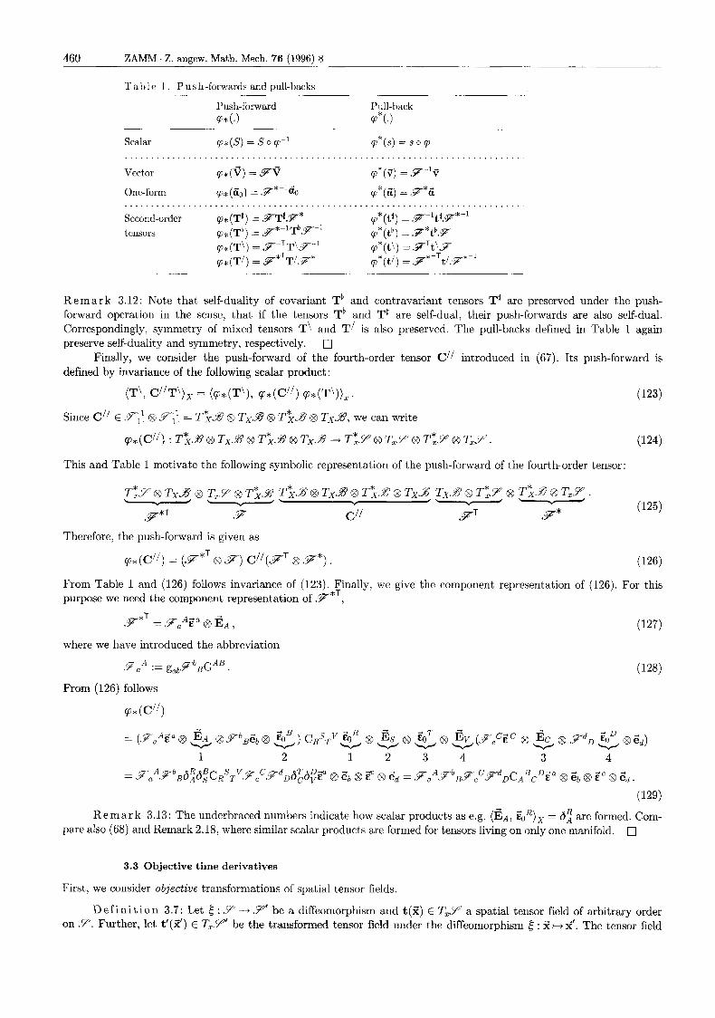
T a b 1 e 1 . P u s h -forwards and pull-backs

Push-forward Pull-back P* (.I P*(.)

Scalar q*(S) = sop-1 P*(.) = s 0 p

Vector p*(3) = F3 P*(5) = . p ' 3

One-form fp* (6") = .F*-'& rp*(6) = 9-*6

Second-order q*(Tn) = ,FT'F* P*(tY) = ; F - I t i y * - l

tensors P* ( ~ 3 ) = p%*-lTb.'F"l p*(tb) = .F*tb.F p*(t\) = .PTtW P*(t/) = ,q*-Tt/.q*-l

. . . . . . . . . . . . . . . . . . . . . . . . . . . . . . . . . . . . . . . . . . . . . . . . . . . . . . . . . . . . . . . . . . . . . . . . . .

. . . . . . . . . . . . . . . . . . . . . . . . . . . . . . . . . . . . . . . . . . . . . . . . . . . . . . . . . . . . . . . . . . . . . . . . . . .

p* (Ti) = sGF-TT\.F-l p*(T/) = .F*TT/.F*

R e m a r k 3.12: Note that self-duality of covariant Tb and contravariant tensors Ts are preserved under the push- forward operation in the sense, that if the tensors Tb and Tr are self-dual, their push-forwards are also self-dual. Correspondingly, symmetry of mixed tensors T\ and T/ is also preserved. The pull-backs defined in Table 1 again preserve self-duality and symmetry, respectively. 0

Finally, we consider the push-forward of the fourth-order tensor Cii introduced in (67). Its push-forward is defined by invariance of the following scalar product :

(T', C/'T'), = (p+(T'), p ( C i i ) p+(T\)), .

Q~*(C/ ' ) : T * X & ' @ T X ~ @ T $ . ~ @ T ~ . $ + T*,Y@TT,.Y @T*,s"@TzY'.

(123)

(124)

Since c// E .T~' 8 yI1 = ~ > d 8 T ~ . W cg ~ $ 2 @ ~ ~ 3 , we can write

This and Table 1 motivate the following symbolic representation of the push-forward of the fourth-order tensor:

TZ.7 @ T x 9 @ TpY @ T%.% T$.H @ Tx.9 @ T>.% @ Tx35 T x 9 €3 T*,.Y @ 1%.9 @ T,Y . - - L '- - + (125) *$T*T 3- C/J .FT .F*

Therefore, the push-forward is given as

rp* (C") = (.F*T €3 .F) C//(.FT @ .F*) .

From Table 1 and (126) follows invariance of (123). Finally, we give the component representation of (126). For this purpose we need the component representation of .F *T ,

.F*T = .Fa+" @ EA,

where we have introduced the abbreviation

.FaA := g,bFb,GAB

From (126) follows

9* (C' / ) 4 - T - +

- @ -

= ( .FaAE'" @ 3 @DhBe'b @ + U

1 2 1 2 3 4 3 4 - A 7 b R B T D - a - fl a. .f R G A G s C R S T V . P ~ C ~ d D g ~ s ~ & @ e'b @ E" @ & = , ~ u A . ~ b R , ~ i r c C ~ d ~ C A ~ ~ D ~ a @ 8i, @ 2' @ & .

(129) R e m a r k 3.13: The underbraced numbers indicate how scalar products as e.g. @ A , Z O ' ) ~ = d; are formed. Com-

pare also (68) and Remark 2.18, where similar scalar products are formed for tensors living on only one manifold. [7

3.3 Objective time derivatives

First, we consider objective transformations of spatial tensor fields.

D e f i n i t i o n 3.7: Let : Y + 9' be a diffeomorphism and t(Z) E TpY' a spatial teitsor field of arbitrary order : 2-2'. The tensor field on 9. Further, let t'(Z') E TnY' be the transformed tensor field under the diffeomorphism

GIESSEN. E. v 4 1 DEK: K O L L i f A N x , F. G.: Dual Variables in Continuum Mechanics. Part 1 461

t ( l ) transforms objectively under the transformation 6 if t’ = t * ( t ) ,

where t* ( t ) is the push-forward o f t under the diffeomorphism 5. D e f i n i t i o n 3.8: We say that the tensor field t(2) is spatially covamant, if (130) holds for every diffeomorphisni

Special cases of diffeomorphism 6 : .Y -+ Y’ are zsometries which leave the metric tensor g invariant. t : . Y +/’. 0

D e f i n i t i o n 3.9: An isometry is a map 5 : Y -+ Y with

4.k) = g .

R e m a r k 3.14: We note that rigid body motions are special cases of isometries. Let q(t) : T/ + T p Y , t 2 0 E R, be an orthogonal tensor and Z ( t ) E Tz,Y a vector on .%. Then the transformation

2’ = q t ) + q(t) 2 (132)

is a rigid body motion. The intensively discussed issue of objectivity is equivalent with invariance under rigid body motions.

We first consider time derivatives on the reference configuration. Here we introduce the maternal tzmP derzvatzvr, where we consider a fixed material particle X .

D e f i n i t i o n 3.10: Let Y be an object defined on the reference configuration 3, where Y can be a scalar, a vector, a one-form, or a tensor of arbitrary order. The maternal tame denvatzve of this object Y is defined as

Y:=- . z li (133)

where the index X indicates that the particle X is held fixed during differentiation. 0 R e m a r k 3.15: Material time derivatives will be indicated by a superposed dot. As is well known the material time derivative of any spatial tensor field t(2) is not an objective tensor field.

However, we can derive spatially covariant time derivatives of spatial tensor fields using the notion of Lze derzvatzves. Here we will only consider the Lie derivative induced by the map Q, : 3’ + Y .

0

D e f i n i t i o n 3.11: The Lze dernuatzve of an object I+V defined on the current configuration 9’ is given by

R e m a r k 3.16: In (134) Q,*(.) and p*(.) denote the push-forward operator and the pull-back operator, respec-

We note without proof [l] that Lie derivatives of materially covariant tensors are also materially covariant, i.e., tively, introduced in Section 3.2 (compare also Table 1).

if under the diffeomorphism < introduced in Definition 3.7,

0

t’ = t * ( t ) , (135)

then XGl(t’) = {*(X’-J(t))

R e m a r k 3.17: We mention that there is a more general and rather abstract definition [l, p. 951 of the Lie derivative based on the concept of flow of the velocity field G t . In this paper we use Definition 3.11 which is especially suitable for applications in continuum mechanics. 0

Applications of Lie derivatives will be given in part 2.

4. Summary

In this section we recapitulate the essential results of Part 1 and advantages of the suggested approach. As usual in tensor calculus on manifolds we distinguish between the tangent space Tx.9 and its dual T*X%‘. From objects living in different spaces as e.g. vectors ? E Tx3’ and one-forms 6 E T*,,% only s c a l a r products can be formed. In Section 2.2 we introduce tensors on manifolds. To cover the great variety of higher order tensors we introduce the notions of the

(:)-family of associate tensors (see Definition 2.8) and representative tensor of a -family of associate tensors. In

31a Z . angew. Math. Xlrch.. Bd. 76. H. 8

462 ZAMM . Z. angew. Math. Mech. 76 (1996) 8

Section 2.3 we introduce generalized dual spaces and scalar products formed of tensors living in such dual spaces. In Definition 2.17 we use scalar products to define dual or adjoint tensors. On manifolds with Riemannian metrics i n n e r products can be defined between objects living in the s a m e vector space. Preservation of inner products leads to the definition of transposed tensors (see Definition 2.24).

In Section 3.1 we consider diffeomorphisms between manifolds and introduce mixed two-point tensors (see Defini- tion 3.2). For such tensors transposes (Definition 3.3) and duals (Definition 3.4) can be defined. Of central importance is Section 3.2, where rules for push-forwards and pull-backs of vectors, one-forms and second-order tensors are derived in a systematic manner. The push-forwards and pull-backs are obtained from invariancc requirements imposed on quadratic forms. Our newly developed rules preserve duality and symmetry of second-order tensors (compare Table 1). Section 3.3 gives a short introduction to objective time derivatives which are based on Lie derivatives.

References

1 2 3

4

5

6

7

8 9

10 11

12 13

14

15 16 17

MARSDEN, E.; HUGHES, T. J. R.: Mathematical foundations of elasticity. Prentice Hall, Englewood Cliffs 1983. HILL, R.: Aspects of invariance in solids mechanics. Advances in Appl. Mech. 18 (1978), 1-75. HAUPT, P.; TSAKMAKIS, C.: On the application of dual variables in continuum mechanics. Contin. Mech. Thermodyn. 1 (1989),

SANSOUR, C.: On the geometric structure of the stress and strain tensors, dual variables and objcctive rates in continuum me- chanics. Arch. Mech. 44 (1993), 527-556. BESSELING, J. F.: A thermodynamic approach to rheology. In PARKUS, H; SEDDOV, L. I. (eds.): Irrwersible aspects of continuum mechanics. Springer, Wien 1968, p. 16-53. BOWEN, R.; WANG; C.-C.: Introduction to vectors and tensors - Linear and multilinear algebra. Volume 1. Plenum Press, New York-London 1980. VAN DER GIESSEN, E. : Models in nonlinear thermomechanics - Finite element models and constitutive models for large deformation plasticity. PhD thesis, Delft University of Technology, Delft 1987. TRUESDELL, C.; NOLL, W.: The non-linear field theories of mechanics. Vol. III/3. Springer, Berlin-New York 1965. ABRAHAM, R.; MARSDEN, J. R.; RATIU, T. : Manifolds, tensor analysis and applications. Addison - Wesley Publishing Comp., Read- ing, Mass., 2nd. edition 1983. MISNER, C. W.; THORNE, K. S.; WHEELER, J. A,: Gravitation. W. H. Freeman & Co., San Francisco 1973. KOLLMANN, F. G.; HACKENBERG, H.-P.: On the algebra of two-point tensors on manifolds with applications in nonlinear solid me- chanics. ZAMM 73 (1993), 307-314. DENG, H.; Vu-QUOC,: On the algebra of two-point tensors and their applications. ZAMM (to appear 1996). HACKENBERG, H.-P. : Uber die Anwendung inelastischer Stoffgesetze auf finite Deformationen mit der Methode der Finiten Ele- mente. PhD thesis, Technische Hochschule Darmstadt 1991. GURTIN, M. E.: An introduction to continuum mechanics. Academic Press, New York-London-Toronto-Sydney-San Francisco 1981. KRONER, E. : Allgemeine Kontinuumstheorie der Versetzungen und Eigenspannungen. Arch. Rat. Mech. Anal. 4 (1960) 4, 273-334. LEE, E. H.: Elastic-plastic deformation at finite strains. Trans. ASME, J. Appl. Mech. 36 (1969), 1-6. SIMO, J. C.; ORITZ, M.: A unified approach to finite deformation elastoplastic analysis based on the use of hyperelastic constitutive equations. Computer Meth. Appl. Mech. Eng. 49 (1985), 221-245.

165-196.

Received November 13, 1995, as first part of a revised version of a paper submitted February 23, 1995; rtccepted November 17, 1995

Addresses: Prof. Dr.-Ing. Dr.-Ing. E. h. FRANZ GUSTAV KOLLMANN, Technische Hochschule Darmstadt, Fachgebiet Maschinenelemente und Maschinenakustik, Magdalenenstrafle 4, D-64289 Darmstadt, Germany Prof. Dr. ERIK VAN DER GIESSEN, Laboratory for Engineering Mechanics, P.O. Box 5033, NL-2600 Delft, The Netherlands