Ann. Inst. Statist. Math. Vol. 55, No. 3, 467-485 (2003) (~)2003 The Institute of Statistical Mathematics

ON THE CUSUM OF SQUARES TEST FOR VARIANCE CHANGE IN NONSTATIONARY AND NONPARAMETRIC TIME SERIES MODELS

SANGYEOL LEE 1, OKYOUNG NA 1 AND SEONGRYONG NA 2

1Department of Statistics, Seoul National University, Seoul 151- 7~2, Korea 2Department of Information and Statistics, Yonsei University, Won-Ju, Gangwon-Do, 220-710, Korea

(Received September 17, 2001; revised September 20, 2002)

A b s t r a c t . In this paper we consider the problem of testing for a variance change in nonstationary and nonparametric time series models. The models under consid- eration are the unstable AR(q) model and the fixed design nonparametric regression model with a strong mixing error process. In order to perform a test, we employ the cusum of squares test introduced by Incl~n and Tiao (1994, Y. Amer. Statist. Assoc., 89, 913-923). It is shown that the limiting distribution of the test statistic is the sup of a standard Brownian bridge as seen in iid random samples. Simulation results are provided for illustration.

Key words and phrases: Cusum of squares test, variance change, autoregressive model with unit roots, nonparametric regression model, strong mixing process, weak convergence, Brownian bridge.

1. Introduction

The problem of testing for a parameter change has attracted much attention from many researchers since the parameter change in the underlying model is occasionally observed in actual practice. Since the paper of Page (1955), a vast amount of relevant articles have appeared in the literature; for example, see Hinkley (1971), Brown et al. (1975), Zacks (1983), CsSrg5 and Horvs (1988, 1997), Krishnaiah and Miao (1988), Wichern et al. (1976), Picard (1985), and the articles cited therein. The problem of testing for a variance change has became an important issue in time series analysis since the variance is often interpreted as a risk in econometrics. Incls and Tiao (1994) considered the cusum of squares test for testing for a variance change. Their method has abundant merits since it is essentially a nonparametric test (distribution free), applicable to detecting multiple change points, and easy to understand and implement under a variety of circumstances; for instance, their test has been extended to GARCH (1, 1) models (cf. Kim et al. (2000)) and linear processes (cf. Lee and Park (2001)).

In linear processes a variance change in the observations implies a change in one of the errors and the converse is also true. Thus a test for a variance change can be performed based on the errors rather than the observations themselves. Furthermore, the test based on the errors outperforms the one based on observations since the latter is subject to serious power losses when the data is highly correlated. Thus, if the time series under investigation is stationary and invertible (see Brockwell and Davis (1991), for the definition), then the former is naturally preferred (cf. Park et al. (2000)). In fact, the ease of application of the cusum of squares test lies in the fact that the limiting

467

468 SANGYEOL LEE ET AL.

distribution of the test statistic is the sup of a standard Brownian bridge. It has been shown by Lee and Park (2001) that this result holds for stationary processes, but so far no attempt has been made to investigate its extension to nonstationary processes. The issue is intrinsically interesting and the result, if it turned out to be true, would merit special attention. Motivated by this, we considered the variance change problem in unstable processes (cf. Chan and Wei (1988)).

In this paper, we also deal with a nonparametric time series model taking into con- sideration its practical importance. The nonparametric approach in time series analysis has been advocated by many authors due to its flexibility and robust features when no parametric models are easy to apply to data (see, for example, Truong and Stone (1992), Neumann and Zreiss (1998) and Hafner (1998)). In fact, the nonparametric time series approach has been well appreciated by practitioners as a preliminary search method aimed at establishing a final parametric model. Needless to say, the task of cor- rect modeling requires an analyst to be informed of the possibility of a variance change when she/he speculates as to its presence in given data set. Here we particularly concen- trate on the variance change problem in a nonparametric regression model with a strong mixing error process.

The organization of this paper is as follows. In Section 2, we deal with the variance change test for the errors in AR(q) models, which cover both stationary and nonstation- ary models. In view of the result of Lee and Wei (1999), which shows that the residual empirical process from the AR(q) model with unit root 1 has a non-Gaussian process as its limiting process, one would likely guess that the same phenomenon might occur in this case. However, on the contrary, the Brownian bridge result is shown to remain the same as in Inclgn and Tiao, and the cusum of squares test is still valid in this case. In light of this result, we discuss a goodness of fit test using the empirical process based on the squares of residuals. It is shown that the empirical process in this case converges weakly to a standard Brownian bridge as long as the error distribution has a symmetric density, which is immediately applicable to a Gaussian test.

In Section 3, we consider the variance change problem in a fixed design nonparamet- ric regression model whose error process is geometrically strong mixing. We show that under regularity conditions the cusum of squares test statistic behaves asymptotically the same as with iid random variables.

Finally in Section 4, we report simulation results for our cusum tests introduced in Sections 2 and 3.

2. Test in AR(q) model

In this section we consider the problem of testing for a variance change in the unstable AR(q) model:

(2.1) X t - - / ~ l X t - 1 . . . . . / ~ q X t - q = s

where et are iid random variables with Eel = 0, Ec 2 = a 2 and Ee~ < ec. We assume that the corresponding characteristic polynomial ~ has a decomposition

r = 1 - j31z . . . . . /3qZ q

l

= (1 - z)a(1 + z) b H ( 1 - 2cOSOkZ + z2 )dkr

k=l

CUSUM OF SQUARES TEST FOR VARIANCE CHANGE 469

where a, b, l, dk are nonnegative integers, Ok belongs to (0, ~r) and r is the polynomial of order r = q - (a + b + 2dl + . . . + 2dr) tha t has no zeros on the unit disk in the complex plane.

Let X t = ( X t , . . . , Xt -q+l ) ' , where X t = 0 for all t < 0. Let )1. ~n : X t - l ~ t - 1 E X t - l X t ,

t = l t = l n > q ,

be the least squares es t imate of /3 ---- ( i l l , - . . ,~3q) t based o n X 1 , . . . ,Xn. Then the resid- uals are

^ l

~t = Xt --/3nXt-1, t = 1,. . . , n .

As mentioned earlier, our goal is to test the following hypotheses: H0: the et have the same variance a 2 vs. H i : not Ho. In order to perform a test, we employ the cusum of squares test s tat ist ic T~ based

on the residuals:

1 k n

(2.2) T n - ~/ngr-~ n l<k<_nmaX t ----n t ,

where ^ 2 n - 1 n ^ n t% ---- ~ t = l e4t - ( n-1 Y]~t=l ~2)2. Then we have the following result.

THEOREM 2.1. Under Ho, as n ---+ co,

(2.3) Tn ~ sup IW~ O<u<l

where W ~ denotes a standard Brownian bridge. We reject Ho i f Tn is large.

P R O O F OF THEOREM 2.1. Since

~ 2 __k ~2 --__ 1 k v/~ t n t ~ ~2__n e

t = l t=l

+ E 4 - - - - t = l t = l

and 1

i n a x l < k < n v ~ v a r ( c 2)

it suffices to show that

k Tt

~2 _ ~2 n v / - ~ t t

sup IW~ O<u<l

(2.4)

and

(2.5)

1 t=~l k m a x - - = gt 2 - ~ c~ = OR(l) l<k<n 4?2 t = l

~2 L var(~i~).

470 SANGYEOL LEE ET AL.

Note that

1 t=~ t=~ ~ L e t ) e t max ~t 2 _ e2 1 l<k<n ~ t --~ l<k<nmaX ~ (et -- (it) 2 -~- 2 t = l (~t -- ~- In -~- 2 I In ,

where k n n

1 1 1 I n = m a x E ( ~ t - et) 2 - E ( ~ t - s 2 - E { ( ~ n - t ~ ) ' X t _ l } 2,

l < k < n ~ t = l - - v ~ t = l V ~ t= l

1 k 1 k IIn = m a x - - = t~=l(~t -s = max = ~ ( ~ - - ~ ) ' X t _ , e t . l<k<n k in l<k<n x/n = n

As in Lee and Wei (1999), in order to show the negligibility of In and IIn, we decompose the time series into several components so that each component has its own distinct characteristic roots.

Let

ut = r - B)-aXt,

vt = r + B)-bxt ,

xt(k) = r - 2cosekB + B2)-dkxt, k = 1,. . . , l ,

zt = ~b(B)~ -1 (B)Xt,

where B denotes the back-shift operator. For convenience, set

Ut ---- ( t t t , . . . , U t - a + l ) t, Vt ---- (Vt , . . . ,V t - -b+l) ' ,

Xt(]g ) ~- ( x t ( k ) , . . . , x t_2dk_Fl (k ) ) ' , Zt = ( Z t , . . . , Z t _ r + l ) ' .

Since Xo = 0, we have Uo = Vo -- Xo(1) . . . . . Xo(1) = Zo -- 0. According to Chan and Wei (1988), there exists a q • q nonsingular matrix Q such

that

= ' x't(1),... 4 ( 0 , 4 ) ' Q X~ (4, ~'~, and there exist block diagonal matrices Sn = diag(Jn, Kn, i n ( i ) , . . . ,in(1), Mn) such that

n

(2.6) S ~ Q ~ _ X ~ _ ~ , ~ ' ~ ' t--1 '~5 ~'n t = l

! !

~ p diag Jn ~ - l ~ h _ l J ~ , . . . , M n Zt-l~t-1 t = l t = l

= op(1),

where Jn, K n , L n ( 1 ) , - . . , L n ( l ) , M , are a x a,b • b, 2dl • 2 d l , . . . , 2 d l • 2dl and r x r matrices�9 Moreover, it holds that

/ I - - 1 ^ (Q Sn) (~n - ~) ~P (2.7)

( s ~ - 1 ~ - 1 ~- i~t t = l t= l

( M n l ) - I t= l Z t - l~J t -1 E Z t - l ~ t t = l

CUSUM OF SQUARES TEST FOR VARIANCE CHANGE 471

= Op(1).

Here, for any sequences of r.v.'s {X,} and {Y~}, Xn "-~g Yn means tha t X n - Y n = Op(1). First , note tha t In -- Og(1/v'~), since

n

(2.8) E { (~n -- t~) ' X t -1 }2 : Op(1), t=l

which is due to (2.6) and (2.7). In order to deal with IIn, note tha t

(2.9) SnQ E Xt- le t : t=l

Jn E Ut-ls t=l

k

Mn E zh-let t=l

Then, in view of (2.7) and (2.9), we have tha t

IIn "JR max ( j ~ ) - t , l < k < n ~ "ll"t-lUt-1 t=l

which is no more than

• u t - l e t J . ut_le~ t=l t=l

n k

E ~ - l e t Mn ~- le t t= l t= l

(2.10) ~ (Sn) -1 Ut_l'ltt_ 1 max E t=l t=l l <_k<_n t=l

- I - ' ' ' n t - ~ (Mn I) Z t - l Z t - 1 Zt- le t l<k<nmaX 2;t_1s t , \t=l t=l -- -- t----I

where If" II denotes the Euclidean norm. Since the first term in each summand in (2.10) is Op(1) by Chan and Wei (1988), we only have to deal with the second terms.

Now, we show that

k

(2.11) max J~ E u t - l e t = Op(1). l<k<n t= l

Recall tha t (1 - B)aut = et and u0 = 0. Set ut(j) = (1 - B)a-Jut, j = 0 , . . . , a - 1, and Ut = (ut(a),. . . ,ut(1))'. By (3.13) of Chan and Wei (1988), there exists an a x a matr ix M such tha t M u t = Ut and Jn = N ~ I M where Nn = d i a g ( n a , . . . ,n) . In this case, we have

,

t=l t=l t= l

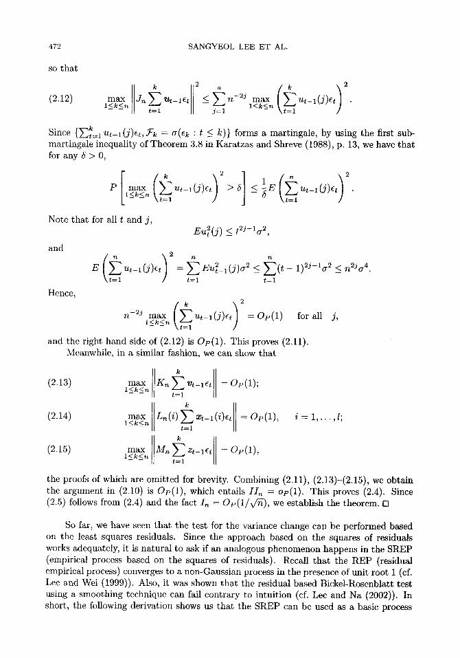
472 S A N G Y E O L L E E E T AL.

so that

) (2 .12) m a x < n - 2 j m a x l < k < n t = l j = l l < k < n t = l

k Since {~-~t----1 U t - l ( j ) ( t , ~ k ~- O' (s : t < k ) } forms a martingale, by using the first sub- martingale inequality of Theorem 3.8 in Karatzas and Shreve (1988), p. 13, we have that for any 5 > 0,

P m a x Ut-l(j)et > 5 < -~E ut-i(j)s l < k < n - - - -

- - t = l

Note that for all t and j ,

and

E

2

Eu2t (j) <<_ t2j-l a 2,

Hence,

n n

---- E Eu~-I(J)a2 <- E ( t - 1)2J-la2 -< n2Ja4" t : l t : l

2

and the right hand side of (2.12) is OF( l ) . This proves (2.11). Meanwhile, in a similar fashion, we can show that

J,

J (2.13) max Kn Vt-let -- OF(l) ; l < k < n

nn(i)~-~ (2.14) max ~-l(i)et : Op(1), i = 1 , . . . , l ; l < k < n t = l

(2.15) max M~ zt- le t = OF(l ) , l < k < n t = l

the proofs of which are omitted for brevity. Combining (2.11), (2.13)-(2.15), we obtain the argument in (2.10) is OR(l) , which entails IIn = OR(l). This proves (2.4). Since (2.5) follows from (2.4) and the fact In -- Op(1 /v /~ ), we establish the theorem. O

So far, we have seen that the test for the variance change can be performed based on the least squares residuals. Since the approach based on the squares of residuals works adequately, it is natural to ask if an analogous phenomenon happens in the SREP (empirical process based on the squares of residuals). Recall that the REP (residual empirical process) converges to a non-Gaussian process in the presence of unit root 1 (cf. Lee and Wei (1999)). Also, it was shown that the residual based Bickel-Rosenblatt test using a smoothing technique can fail contrary to intuition (cf. Lee and Na (2002)). In short, the following derivation shows us that the SREP can be used as a basic process

CUSUM OF SQUARES TEST FOR VARIANCE CHANGE 473

for a goodness of fit test so long as the underlying density is symmetric and satisfies the regularity conditions in Lee and Wei, Section 3.2. The result is directly applicable to a Gaussian test.

Let F be the distribution of el with symmetric density f , and let G be the distri- bution of e~, namely, G(x 2) = F(x) - F ( - x ) for x _> O. Define

n

1 ~ { I ( 4 _ < x ~ ) - a ( x ~ ) } , x > 0 , En(x) = ~ ~:1

n

~ { i ( ~ < x~)-a(x~)}, ~ > 0. 2n(X) : - ~ ~=1

Then,

g~(x) - 1 n

) - ~ { i ( - x < ~ < x) - (F(x) - F ( - x ) ) } v~

n 1 n 1 E { i ( g t <_ x ) - F(x)} - ~ ~-'~{I(~t <_ - x ) - F ( - x ) } .

V/n t ~ l =

Since in view of Lee and Wei (1999),

n

1 ~{• _< x ) - F(x)} - V/n t= l

n

1 E { i ( e t _< x ) - F(x)} V/n t = l

n

1 ~ ( ~ _ ~) 'x~_ iI (x ) + ~ ( x ) -[- " ~ t = l

with SUpx I~n(X)l = Op(]-), and f (x) = f ( - x ) , we can see that

sup Ign(X) - - ~n(X)] = Op(1). x

Therefore, gn(U) := $,((G-I(u)) 1/2) ~ W~ 0 < u < 1.

The above result suggests that a goodness of fit test for a symmetric density, includ- ing a Gaussian test, can be accomplished based on gn- In fact, the Gaussian test (when the variance is known) is converted into a chi-square distribution test. In actual practice, one should keep in mind that, if an estimate of variance is plugged into the empirical process, the limiting distribution is no longer a Brownian bridge, but a Gaussian process as we usually observe in the empirical process context (cf. Lee and Wei (1999), Section 3.2). Besides the goodness of fit test, we can reason that the sequential SREP (cf. Bai (1994)) can be employed to detect a distributional change in autoregressive models un- der the same conditions; it is well-known that this result does not hold when using the sequential REP (cf. Ling (1998)). All these facts support the usefulness of the method employing the squares of residuals in autoregressive models.

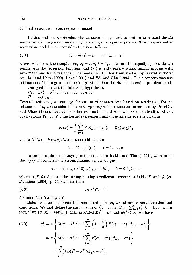
474 S A N G Y E O L L E E E T AL.

3. Test in nonparametric regression model

In this section, we develop the variance change test procedure in a fixed design nonparametr ic regression model wi th a strong mixing error process. The nonparametr ic regression model under consideration is as follows:

(3.1) Y, = g(xt) + e,, t = 1 , . . . , n ,

where n denotes the sample size, x t = t / n , t = 1 , . . . , n, are the equally-spaced design points, g is the regression function, and {et} is a s ta t ionary strong mixing process with zero mean and finite variance. The model in (3.1) has been studied by several authors: see Hall and Hart (1990), Har t (1991) and Wu and Chu (1994). Their concern was the est imation of the regression function g ra ther than the change detection problem itself.

Our goal is to test the following hypotheses: H0: Eet 2 = a 2 for all t = 1 , . . . , n vs. H1: not H0.

Towards this end, we employ the cusum of squares test based on residuals. For an est imator of g, we consider the kernel-type regression est imator introduced by Priestley and Chao (1972). Let K be a kernel function and h -- hn be a bandwidth. Given observations Y1,- .- , In , the kernel regression function est imator gn( ' ) is given as

1 n = - ~ - ~ Y t g h ( x - x t ) , 0 < x < 1, gn(x)

t = l

where K h ( u ) = K ( u / h ) / h , and the residuals are

et = Yt - g n ( x t ) , t = 1 , . . . , n .

In order to obtain an asymptot ic result as in Incls and Tiao (1994), we assume tha t {et} is geometrically strong mixing, viz., if we put

ak = a ( a ( e s , s < O ) , a ( e s , s > k)), k = 0, 1 , 2 , . . . ,

where a(.T, 6) denotes the strong mixing coefficient between a-fields 9 c and G (cf. Doukhan (1994), p. 3), {ak} satisfies

(3.2) ak ~ C e -pk

for some C > 0 and p > 0. Before we state the main theorem of this section, we introduce some notat ion and

k conditions. We first define the part ial sum of e~, namely, Sk = ~-,t=l e2t, k = 1, . . . , n. In 2 Var(S~), then provided E ~ = a 2 and Ee 4 < c~, we have fact, if we set s n =

2 E(e 2 - a 2 ) 2 2 ~ 1 - Z ( c ~ - a 2 ) ( e 2 + k - a 2) (3.3) 8 n = n + k = l

n

- 2)--:. - - : ) , k = l

CUSUM OF SQUARES TEST F O R VARIANCE CHANGE 475

which is useful for later work. Since we have to deal with the residuals, we also define the partial sum of residuals:

S k = E @2 for t=[nhl+ l

k = [nh] + 1 , . . . , n - [nh],

where the truncations for k are concerned with the kernel function K satisfying 2 2 2 supp(K) C [-1, 1] which is assumed in (A3) below. Moreover, v(k) := E(el - a )(ei+ k -

a 2) is estimated by

1 "~(k) - n - 2 [ n h ] E (e2_ ^ ^2

t=[nh]+l

where 1 n-[nh]

- n - 2[ h] t=[nh]+l

Then the estimator sn̂ 2 of Sn2 is given by

~̂ {~( S n = It O)

n } ,

k=l

for a sequence of positive integers {/n} satisfying In --* oo and I n / n --* 0 as n --* c~ as will be explained in more detail shortly. Note that the residuals near end points are discarded to avoid the boundary effect in nonparametric regression.

Below are the conditions imposed in this section. (A1) { a k } satisfies (3.2), and Ele 2 - a2I r < c~ for some r > 2. (A2) The regression function g satisfies the Lipschitz condition, viz.,

Ig(x) - g (y ) l < D l l x - y l , O <_ x , y <_ l

for some constant 0 < D1 < oo. (A3) The kernel function K vanishes outside [-1, 1] and is Lipschitz continuous

on [-1, 1], viz., I K ( x ) - K ( y ) I <_ D21x - Yl, - 1 <_ x , y < 1

for some constant 0 < D2 < c~. And K satisfies f K ( x ) d x = 1.

(A4) The bandwidth h = hn satisfies n h 2 -~ c~ and n h 4 --* 0 as n -~ c~.

(Ah) In satisfies In -~ cx~, l n / v / ~ h -~ 0 and l ~ h -~ 0 as n -~ ~ .

R e m a r k . A broad class of processes, including invertible stationary ARMA(p, q) processes with innovations having a continuous distribution, satisfy Condition (A1) (cf. Gorodetskii (1977)). Conditions (A2)-(A4) are the usual conditions assumed in non- parametric regression estimation.

Here is the main result of this section.

476 SANGYEOL LEE ET AL.

THEOREM 3.1. Assume that Ho holds. Under Conditions (A1)-(A5),

(3.4) T~* := max S k - ~ sup I w ~ . [nhl+ l <_k<_n--[nh] -- 0<u<t

We reject Ho if T~ is large.

Now we prove Theorem 3.1. We start with a lemma which can be found in Doukhan ((1994), p. 46).

LEMMA 3.i. Assume that Ho holds. I f E]e~ - a21 ~ < c~ for some r > 2 and (3.2) is true for some C > 0 and p > O, then

(3.5) Z ( ~ [ n . ] - -~ W O.

LEMMA 3.2. Under Ho and

1 ^ max gkl ~ o, I S k -

[nh]+l~k<n-[nh] x/n

k where Sk = Et=[nh]+l e2t"

PROOF. We write k 1 ~ 1

t=[uh]+l k k

1 2 1

t=[nh]+ l V/~ t=inh]+ l

= I k + I I k .

Observe that .-[nh] {

1 1 s -- Xj) (3.6) Ia <_ ~ E n t=[nh]+l

< 3

2

+ - ~ g ( ~ j ) K . ( x ~ - ~ j ) - g(xd It j=l

-~1 ~_, nl ejKh(xt -- xj) t=[nh]+l j=l

in nhJ{l }2 + . ~ ~ (g(xj) - g(x~))K.(x~ - xj)

t=[nh]+l "=

.

CUSUM OF SQUARES TEST FOR VARIANCE CHANGE 477

It is easy to check tha t the first t e rm in (3.6) is O p ( n - t / 2 h -~) since

E ej K h (x t - x j ) = 0 ,

due to (A1) and (A3). The remaining nonstochastic terms in (3.6) are of order O ( n l / 2 h 2) and O(n-3 /2h -2 ) , respectively, since

and

n s ~ , ( g ( . , ) - a (x~))Kh( .~ - ~ ) = O(h) n

j = l

(3.7) g(xt) K h (x t - x j ) - 1 = 0 , j = l

where we have used (A2) and (A3). Then, by using (A4) we obtain

(3.8) max Ilkl = oF( i ) . [nh]+ l <_k<n-[nh]

For I Ik , we decompose it into three terms as follows:

{ ( )} ---- V 1~2 t=~nh]+l g(xt) 1-- X E Kh(x t -- s I Ik

--e2 ~-..~ 1 ~ ( g ( x ~ ) - g (x , ) )Kh(x~ - x , ) + v~e t=[~]]+ l n j=l

} t=[nh]+l rt j = l

= IIk,1 -}- I I k a -- IIk,3.

First, observe tha t

2 n-fnh]

III<ll <_ -~ t=[n~h]q_l

From this and (3.7), we have

) g(xt) 1 - - 1 K h ( x t - - x j ) n

j = l

s

(3.9) max [IIk,11 = O p ( n - 1 / 2 h - 1 ) �9 [nhl+l<_k<n-[nh]

For IIk,2, set p = [n 1/3] and q = [(logn)2], and define random variables V / a n d y~, as follows:

bi ai+l --1 [,~ - 2 I~h] ] ~ = ~ , ~'= ~ ~, ~=l,...,r= ~Tq j' t=ai t=bi-k l

478 SANGYEOL LEE ET AL.

(3.11)

since

--1 n [nh] + 1 + (p + q)(i 1) and where ~Tt = (n Y~.j=l(g(xt) - g(x j ) )Kh(x t - xj))et , ai = bi = [nh] + 1 + (p+ q)(i - 1) +p . Then, we can write

~Zk 2 k 2 ~k 2 V/ 2 (a. lo) ss~,2-~ ~ ~ , = ~ Z ~ + ~ ,+~/'k, t=[nh]+l 7=1 i = 1

k where uk is the largest integer such that [nh]+l+uk(p+q) <_ k, and Ak = Y~.t=[nh]+l rh-- Uk Uk Y~-i=l 17/- ~--~-~=1 IX/'. Let ~ be any positive real number. By the coupling theorem (cf.

Doukhan (1994), p. 8, and Bosq (1996), p. 18), there exist independent random variables VI*,... , V* such that Vi* and 17i have the same distribution and

( ( P IV~-V~*l >r < 1 8 aq 2

Then, we can see that

max = op(1), [nh]-t- l <--k<--n--[nhl

t inh]+ l <-k<-n-[ nh]

< P max Vi > - k,~_~_~-~ < P ( m a x 1 E V / * - kl<~_<~ 7 ( > + P max V i - V i * )

l<u<r

P ( max 1 IAkl > r \[nhl+l<k<_n-[nh]

<_ P max rh i = 1 ai <k<ai+ l--1

- - t ~ i

(r (p + q)m = 0 \ n~ 2 ) ,

>

~ ~--~ Var V/* + IV/- V/*I > )

i = 1 i = 1

__ o + o t,/~) )

= o(1). In the same manner, we also get

1 ~ If/' (3.12) max = op(1). [nhl+l <k<n-[nh] V ~

Furthermore, applying the coupling theorem again, we can show that for any ~ > 0,

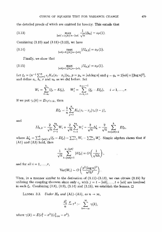
C U S U M OF SQUARES T E S T F O R V A R I A N C E C H A N G E 479

the detailed proofs of which are omit ted for brevity. This entails tha t

(3.13) 1 max IAal = OF(l). [nh]+l<k~n-[nh] V/~

Combining (3.10) and (3.11)-(3.13), we have

(3.14) max Iz/k,21 = op(1). [~h]+l<k<~-[nh]

Finally, we show tha t

(3.15) max IIIk,31 = OF(l). [nh]+l~_k~n-[nh]

n Let ~t = (n -1 ~-~j=l c jKh(Xt - -x j ) )e t , p = Pn = [nhlogn] and q = qn = 2[nh] + [(logn)2], and define ai, bi, r and uk as we did before. Set

b~

w, = ~ (~ - E6) , w : : t=a~

a i + l - - 1

( ~ - E~,), t=biA-1

i = 1 , . . . , r .

If we put 7~(k) = E ~ l ~ l + k , then

and

n

= -

j = l

2 ~ 2 _ ~ 2 ~ , 2 IIk,3 = - - ~ E Wi + W: + + E~t,

t k Uk uk = - - }-~-i=1 Wi shows tha t if - ~-~i---1 W[. Simple where A k ~-~n=[nh]+l (~t E~t) algebra (A1) and (A3) hold, then

n-[nh]

t=[nh]+l

and for all i = 1 , . . . , r ,

Var(Wi) = O \ n2h2 ] .

Then, in a manner similar to the derivation of (3.11)-(3.13), we can obta in (3.15) by utilizing the coupling theorem since only ej with j = t - [ n h ] , . . . , t + [nh] are involved in each ~t- Combining (3.8), (3.9), (3.14) and (3.15), we establish the lemma. El

LEMMA 3.3. Under 1to and (A1)-(Ah), as n ~ c~,

^2 co

n k ~ - o o

where ~(k) = E ( ~ - ~)(~1~+~ - ~2).

480 S A N G Y E O L LEE E T AL.

PROOF. Let

~/*(k) = (n - 2[nh]) -1 n - [ n h l - N

E (c2 e2 - ' - # 2 ) ( t+lkl tt2) t=[nh]+l

where #2 (n 2[nh])_l v-.n-[nhl 2 = -- 2--,t=ir~h]+l et" It suffices to show that

In In

(3.16) E ~ ( k ) - E "~*(k) p 0 k=-l~ k=-l~

and In In

(3.17) E " / * ( k ) - E "~(k) P o" k=-ln k=-l,~

In order to verify (3.16), we write

1 ~(k) - ~,*(k) - n - 2[nh]

n-[nh]-k

- - - c ~ ) ( E , + k - - ~ 2 )

t=[nhl+l + (e~ ~ ) ( ~ f ,2) + ( 4 .2 _ _ _ _ . ~ ) ( ~ , § ~+~)

+ ( d ~ 2 ) ( ~ f,~) + ( .2 - ~ ^5 - - ~ ) ( ~ + ~ - 4 + ~ )

+ (#2 - ^ 2

= R l ( k ) + . . . + R s ( k ) .

Observe that by the Schwarz inequality,

n-[nh] 1

]Rl(k)l-< n - 2 [ n h ] E (e2-~t2)2 t=[nh]+l n-[nh]

2 < . r L , ~ ( g ~ ( x , ) - - g ( ~ ) ) 4 + - n - z/nnu

t J t=[nh]+l

n-[~hl 8 y- - g ( ~ ) ) ~ , .

n - 2 [nh l t=[nh]+l By Jensen's inequality and Condition (A1), we can see that

n--[nh] rt~h] { (1~.~= 1 )4 (gn(x~) - g ( x d ) 4 < 27 - ~ j K h ( x , - x j )

t=[nh]+l t=[nhJ+l 4

+ - ~ ( g ( x j ) - g ( x ~ ) ) K h ( x ~ - z j ) n j=l

n 1 n 1 +o,o 4, + o

CUSUM OF'SQUARES TEST FOR VARIANCE CHANGE 481 E v ' n - [nh] Since z--,t=[nh]+l e4t = O(n ) and

n-[nh] E (gn(Xt) 22 - g ( x t ) ) et <

t=[nh]+l

we obtain, uniformly in k,

( 1 (3.18) [R~(k)[ = ON

( n~_~h] )1/2 (rt~_~h ] )1/2 (gn(xt) - g (x t ) ) 4 e 4 ,

\t=[nh]+l \t=[nh]+l

/ ( ( 1 / 1 / 2 ) (1) V h 4 + O R n--~-gh2Vh 4 = O R -s v h 2 ,

where a V b denotes the maximum of a and b. For i = 2, 4, we have

(3.19) n- [nh] )

IRi(k)l < 1 t=[nh]+l

1/2

n--[nh] ) 1/2 1 [ 2 p2) 2

t=[nh]-t-1

(Op(-~l h2)) 1/2 = V ( ())Op1 1/2

) = Op V h

in view of (3.18). Furthermore, by Lemma 3.2, we have that for i = 3,6,

(3.20) Ini(k)[ <

and for i = 5, 7,

(3.21) IRi(k)l <

= op

Also, by Lemma 3.2,

(3.22)

n 1 max ( n - 2[nhD 2 [nh]+Z<_j<_n-[nh] V ~

1 n ~ h ] (e~ - d )

v/-d t=[,~hl+l

1 n - [nh]

n - 2[nh] t=[nh]+l

o,(1) n

(n - 2[nh]) 2

J

t=[nh]A-1

n - 2[nh] ( ~ -

( rn j r)2 1 E (et2 - gt2)

"-~ t=[nh]+l

482 S A N G Y E O L LEE E T AL.

Hence, (3.16) is yielded by (3.18)-(3.22) and Condit ion (A5). Now, it remains to prove (3.17). Noticing tha t

1 n-[nh]-k

-- @t ~t+k t=[nh]+l

n - 2[nh] +

n - 2[nh] (t=[nh]+l t=n-[nh]-k+l

we have

k 2 2 n -- 2[nh] (EClel+k nu vr4)

n - [n h] - k I. 1 -- (etet+ k -- Ee2te2+k ) + OR(l). E ('~*(k) 7(k)) -- 2[nh] E 22

k=--ln k=-ln n - t=[nh]+l

Then, using the Minkovski inequality in L2-norm [l" [12, and Conditions (A1) and (A5), we obtain

n-- [nh] - - k [ 1

@t 6t +k n - 2[nh] Z 22 _ Ee2e2t+k) k=-ln t=[nh]+l 2

l. ] 1 -< E n - 2[nh] E

t=-ln t=[nh]+l nhlk 2 II (etet+ k - Ee2e2+k )

2

= o p ( 1 ) ,

which implies (3.17) and the lemma is established. []

P R O O F OF T H E O R E M 3.1. Let -2 S n = Var(Sn_[nh] ). Then, from (3.3) and Lemma

3.3, we can see tha t Sn/Sn P 1 and ~n/v/-n P T. Now, note tha t

k - [nh] ~ ls~ Sk - n - 2[nh] --[-hl)

} sn gn n - 2[nh] n-[nh]

Sn V ~ (~k -- ~k) ~ - - - 2 - ~ 1 (S--Inhl -- Sn-l-hJ) �9

Then, the theorem is a direct result of Lemmas 3.1 and 3.2. []

4. Simulation results

In this section we conduct a simulation s tudy to evaluate the tests in Sections 2 and 3. In this simulation we perform a test at a nominal level a = 0.05. The empirical

CUSUM OF SQUARES TEST FOR VARIANCE CHANGE 483

sizes and powers are calcula ted as the reject ion number of the null hypothes is out of 2000 repet i t ions. First , in order to see the pe r fo rmance of Tn in Sect ion 2, we consider the model

X t = f lX t -1 + et, t = 1 , . . . , n ,

where X0 is assumed to be 0 and r are lid normal r a n d o m variables wi th m e a n zero and variance a 2. Now we consider the p rob lem of tes t ing the following hypotheses:

H0: cr 2 remains equal to 1 for t = 1 , . . . , n, vs. H i : ~r 2 = 1 for t = 1 , . . . , [ n / 2 ] and a 2 = A for t = [n/2] + 1 , . . . , n ,

where A takes the values 2 and 4. Here we evaluate Tn wi th the sample size n = 200, 300, 500 and fl = 0.2, 0.5, 0.8, 1.0. The empir ical sizes and powers are summar ized in Table 1. As seen in the table, Tn does not have size dis tor t ions and produces good powers. I t is manifes t t ha t the sizes and powers do not depend upon the values of fl, and the test works well for the uns table case as well as the s t a t i ona ry case.

Now, in order to evaluate the pe r fo rmance of the test T,~ in Sect ion 3, we consider the nonpa rame t r i c regression model in (3.1):

Yt = g(x t ) -b ~t, t = 1 , . . . , n,

where g(x) = 25x 3 - 45x 2 + 24x - 3.6 and {~t} satisfies the equation:

r ~-- r -]- et, Ir < 1, t = 1 , . . . , n,

where et are lid normal r a n d o m variables wi th mean zero and var iance w 2. For the es t imat ion of the regression function, we use the kernel funct ion

K ( x ) = ~(1 - x2) I [_ l ,1] (x ) ,

where I(-) denotes the indicator function, the bandwid th h = hn = n - 1 / 3 / 3 , and In = 2 As before, we assume tha t the var iance change occurs a t t = n / 2 [n 1/4] in es t imat ing s , .

and pe r fo rm a test for the following hypotheses: H0: w 2 remains equal to 1 over t = 1 , . . . , n , vs. H i : w 2 changes f rom 1 to 8 at t = In/2],

where 5 takes the values 2, 4 and 9. Here we employ the sample size n -- 200, 300, 500, and r = 0, 0.3, 0.5, 0.8 in order to see the correlat ion effect. T h e figures in Tables 2 and 3 denote the empir ical sizes and powers, respectively. From the results , we can see t ha t the tes t has no severe size dis tor t ions at m o d e r a t e sample size, say, n > 300, and it produces good powers u n d e r / / 1 . T h e power depends on the values of r which decreases as r approaches 1 and when 5 has lower values. As ant ic ipated, it increases as ei ther 5 or n increases. The results ob ta ined in our s imulat ion s tudy enable us to conclude t ha t the cusum of squares test pe r fo rms adequa te ly for the var iance change in nons t a t iona ry and nonpa rame t r i c t ime series models.

Table 1. Empirical sizes and powers of Tn.

/3 0.2 0.5 0.8 1.0

A size 2 4 size 2 4 size 2 4 size 2 4

200 .033 .818 1,00 .030 .818 1.00 .037 .788 1.00 .037 .826 1.00

300 ,034 .953 1.00 .039 .953 1.00 .032 .953 1.00 .037 .957 1.00 500 .042 .998 1.00 .050 .997 1.00 .042 1.00 1.00 .042 .998 1.00

484 SANGYEOL LEE ET AL.

Table 2. Empirical sizes of T~.

r 0.0 0.3 0.5 0.8

200 .028 .030 .035 .030

300 .026 .034 . 0 4 1 .040

500 .034 .048 .042 .050

Table 3. Empirical powers of T n.

r 0.0 0.3 0.5 0.8

2 4 9 2 4 9 2 4 9 2 4 9

200 .559 .981 .998 .511 .978 .998 .466 .949 .995 .318 .851 .978

n 300 .834 1.00 1.00 .774 .999 1.00 .706 .995 1.00 .474 . 9 6 1 .996

500 .990 1.00 1.00 .975 1.00 1.00 .940 1.00 1.00 .725 .999 1.00

Acknowledgements

We like to thank the referees for their valuable comments. This research was sup- ported (in part) by KOSEF through Statistical Research Center for Complex Systems at Seoul National University.

REFERENCES

Bai, J. (1994). Weak convergence of the sequential empirical processes of residuals in ARMA models, Ann. Statist., 22, 2051-2061.

Bosq, D. (1996). Nonparametric Statistics for Stochastic Processes; Estimation and Prediction, Lecture Notes in Statist., Springer, New York.

Brockwell, P. J. and Davis, R. A. (1991). Time Series: Theory and Methods, 2nd ed., Springer, New York.

Brown, R. L., Durbin, J. and Evans, J. M. (1975). Techniques for testing the constancy of regression relationships over time, J. Roy. Statist. Soc. Set. B, 37, 149-163.

Chan, N. H. and Wei, C. Z. (1988). Limiting distribution of least squares estimates of unstable autor~ gressive processes, Ann. Statist., 16, 367-401.

CsSrgS, M. and Horvgth, L. (1988). Nonparametric methods for change point problems, Handbook of Statistics (eds. P. R. Krishnaiah and C. D. Rao), Vol. 7, 403-425, Elsevier, New York.

CsSrgS, M. and Horv~th, L. (1997). Limit Theorems in Change-point Analysis, Wiley, Chichester. Doukhan, P. (1994). Mixing: Properties and Examples, Springer, New York. Gorodetskii, V. V. (1977). On the strong mixing properties for linear sequences, Theory Probab. Appl.,

22, 411-413. Hafner, C. M. (1998). Nonlinear Time Series Analysis with Applications to Foreign Exchange Rate

Volatility, Physica, Heidelberg. Hall, P. and Hart, J. D. (1990). Nonparametric regression with long range dependence, Stochastic

Process. Appl., 36, 339-351. Hart, J. D. (1991). Kernel regression estimation with time series errors, J. Roy. Statist. Soc. Ser. B,

53, 173-187. Hinkley, D. V. (1971). Inference about the change-point from cumulative sums tests, Biometrika, 58,

509-523.

Incls C. and Tiao, G. C. (1994). Use of cumulative sums of squares for retrospective detection of changes of variances, J. Amer. Statist. Assoc., 89, 913-923.

Karatzas, I. and Shreve, S. E. (1988). Brownian Motion and Stochastic Calculus, Springer, New York.

CUSUM OF SQUARES TEST FOR VARIANCE CHANGE 485

Kim, S., Cho, S. and Lee, S. (2000). On the cusum test for parameter changes in GARCH(1,1) models, Comm. Statist. Theory Methods, 29, 445-462.

Krishnaiah, P. R. and Miao, B. Q. (1988). Review about estimation of change points, Handbook of Statistics (eds. P. R. Krishnaiah and C. P. Rao), Vol. 7, 375-402, Elsevier, New York.

Lee, S. and Na, S. (2002). On the Bickel-Rosenblatt test for first order autoregressive models, Statist. Probab. Lett., 56, 21-35.

Lee, S. and Park, S. (2001). The cusum of squares test for scale changes in infinite order moving average processes, Scand. J. Statist., 28, 625-644.

Lee, S. and Wei, C. Z. (1999). On residual empirical processes of stochastic regression models with applications to time series, Ann. Statist., 27, 237 261.

Ling, S. (1998). Weak convergence of the sequential empirical processes of residuals in nonstationary autoregressive models, Ann. Statist., 26, 741-754.

Neumann, M. H. and Kreiss, J. P. (1998). Regression-type inference in nonparametric autoregression, Ann. Statist., 26, 1570-1613.

Page, E. S. (1955). A test for change in a parameter occurring at an unknown point, Biometrika, 42, 523-527.

Park, S., Lee, S. and Jeon, J. (2000). The cusum of squares test for variance changes in infinite order autoregressive models, J. Korean Statist. Soc., 29, 351-361.

Picard, D. (1985). Testing and estimating change-points in time series, Advances in Applied Probability, 17, 841--867.

Priestley, M. B. and Chao, M. T. (1972). Non-parametric function fitting, J. Roy. Statist. Soc. Ser. B, 34, 385-392.

Truong, Y. K. and Stone, C. J. (1992). Nonparametric function estimation involving time series, Ann. Statist., 20, 77-97.

Wichern, D. W., Miller, R. B. and Hsu, D. A. (1976). Changes of variance in first-order autoregressive time series models--with an application, Appl. Statist., 25, 248-256.

Wu, J. S. and Chu, C. K. (1994). Nonparametric estimation of a regression function with dependent observations, Stochastic Process. Appl., 50, 149-160.

Zacks, S. (1983). Survey of classical and Bayesian approaches to tile change-point problem: Fixed sample and sequential procedures of testing and estimation, Recent Advances in Statistics (eds. M. H. Rizvi, J. S. Rnstagi and D. Siegmund), 245 269, Academic Press, New York.