On The Numerical Solution of Linear Fredholm-Volterra ...€¦ · Hence, the matrix representation...

556

Available at http://pvamu.edu/aam

Appl. Appl. Math.

ISSN: 1932-9466

Vol. 7, Issue 2 (December 2012), pp. 556 - 570

Applications and Applied Mathematics:

An International Journal (AAM)

On The Numerical Solution of Linear Fredholm-Volterra İntegro Differential Difference Equations With Piecewise İntervals

Mustafa Gülsu and Yalçın Öztürk

Deparment of Mathematics Mugla University

Mugla,Turkey [email protected]; [email protected]

Received:August 03, 2011; Accepted: October 6, 2012

Abstract The numerical solution of a mixed linear integro delay differential-difference equation with piecewise interval is presented using the Chebyshev collocation method. The aim of this article is to present an efficient numerical procedure for solving a mixed linear integro delay differential difference equations. Our method depends mainly on a Chebyshev expansion approach. This method transforms a mixed linear integro delay differential-difference equations and the given conditions into a matrix equation which corresponds to a system of linear algebraic equation. The reliability and efficiency of the proposed scheme are demonstrated by some numerical experiments and performed on the computer algebraic system Maple 10.

Keywords: Mixed linear integro delay differential-difference equations; Chebyshev polynomials and series; Approximation methods; Collocation points

MSC 2010 No.: 41A58; 39A10; 34K28; 41A10

1. Introduction In recent years, the studies of mixed integro delay differential-difference equations have developed very rapidly. These equations may be classified into two types; the Fredholm integro-differential-difference equations and Volterra integro-differential-difference equations. The upper bound of the integral part of Volterra type is variable, while it is a fixed number for that of

AAM: Intern. J., Vol. 7, Issue 2 (December 2012) 557

Fredholm type. In this paper we focus on Fredholm Volterra integro differential difference equations with piecewise intervals. Integro-differential-difference equations are important, but are often harder to solve, even numerically, and progress on how to solve them has been slow. Problems involving these equations arise frequently in many applied areas including engineering, mechanics, physics, chemistry, astronomy, biology, economics, potential theory, electrostatics, etc. [Emler (2001,2002), Ren (1999), Rashed (2004), Kadalbajoo (2002,2004), Bainov (2000), Cao (2004),]: The study of integro differential difference equations has great interest in contemporary research work. Several numerical methods, such as the successive approximations, Adomian decomposition, Chebyshev and Taylor collocation, Haar Wavelet, Tau and Walsh series methods, etc. [Ortiz (1998), Hosseini (2003), Zhao (2006), Maleknejad (2006), Sezer (2005a, 2005b), Synder (1966), Gülsu (2010)] are used for their solution. Mainly we deal with the following integro delay differential-difference equation with piecewise intervals

v

j

x

a

jj

u

i

b

a

ii

n

s

ss

m

k

kk

j

i

i

dttytxKdttytxF

xgxyxHxyxP

00

0

)(

0

)(

)(),()(),(

)()()()()(

(1)

]0,[ x , 1,,1 jii cba under the mixed conditions

1,...1,0,0,)(1

0 0

)(

miccyc ij

m

ki

r

jij

kij

k , (2)

where )(xy is an unknown function, the known )(xPk , )(xH s , ),( txFi , ),( txK j and )(xg are

defined on an interval and also kijc , ijc , i and s are appropriate constant. Our aim is to find an

approximate solution expressed in the form

N

rrr xTaxy

0

)()( , 0 i N , (3)

where Nrar ,...,2,1,0, , are unknown coefficients and N is any chosen positive integer such that mN . To obtained a solution in the form(3) of the problem (1) and (2), we may use the collocation points defined by

NiN

ixi ,,2,1,0,)cos(1

2

. (4)

The remainder of the paper is organized as follows: Higher-order linear mixed integro-delay-differential-difference equation with variable coefficients with piecewise intervals and fundamental relations are presented in Section 2. The method of finding approximate solution is described in Section 3. To support our findings, we present numerical results of some experiments using Maple10 in Section 4. Section 5 concludes this article with a brief summary.

558 M. Gülsu and Y. Öztürk

2. Fundamental Matrix Relations Let us write Eq.(1) in the form

v

jjj

u

iii xJxIxgxHxD

00

)()()()()( ,

where the differential part

m

k

kk xyxPxD

0

)( )()()(

and the difference part

n

s

ss xyxHxH

0

)( )()()(

the Fredholm integral part

dttytxFxIi

i

b

a

ii )(),()(

and Volterra integral part

dttytxKxJx

c

jj

j

)(),()( .

We convert these equations and the mixed conditions in to the matrix form. Let us consider the Eq. (1) and find the matrix forms of each term of the equation. We first consider the solution

)(xy and its derivative )()( xy k defined by a truncated Chebyshev series. Then we can put series in the matrix form

AT )()( xxy , AT )()( )()( xxy kk , (5)

where

)](...)()([)( 210 xTxTxTx T , )](...)()([)( )()(1

)(0

)( xTxTxTx kN

kkk T , TNaaa ]...[ 10A .

On the other hand, it is well known that [Synder (1966)] the relation between the powers nx and the Chebyshev polynomials )(xTn is


,11,)(2

20

2122

xxTjn

nx

n

jj

nn (6)

and

.11,)(12

20

12212

xxT

jn

nx

n

jj

nn (7)

Using the expression (6) and (7) and taking Nn ...,,1,0 , we obtain the corresponding matrix relation as follows:

)()( xx TT DTX and ,))(()( 1 Txx DTX (8)

where

TNxx ]...1[ 1X . for odd N,

NN N

N

N 11

11

0

1

20

022/)1(

0

020

202

1

2

2

1

0020

10

00020

0

2

1

D

and for even N,

NNN N

N

N

N

N 111

11

0

1

20

22/)2(

022/2

1

020

202

1

2

2

1

0020

10

00020

0

2

1

D .


Then, by (8), we obtain

1))(()( Txx DXT (9)

and

1))(()( T(k)(k) xx DXT , ,...2,1,0k . (10)

Moreover it is clearly seen that the relation between the matrix )(xX and its derivative )(x(k)X is

kk) xx BXX( )()( , (11)

where

0000

0000

0200

0010

N

B .

2.1. Matrix Representation for Differential and Difference Parts Let us assume that the function )(xy and its derivatives have truncated the Chebyshev expansion of the form

N

r

krr

k mkxTaxy0

)()( .,...,2,1,0),()( (12)

The derivative of the matrix )(xT defined in (10), and the relations (11), give

1))()( Tk(k) xx (DBXT . (13)

Substituting (13) into (5) we obtain

A)(DBXAT 1)()( )()()( -Tkkk xxxy , (14)

where )(),...,(),(),()(),()( 10)0()0( xTxTxTxTxTxyxy N are first-kind Chebyshev polynomial,

Naaa ,...,, 10 are coefficients to be determined in (3). Now, the matrix representation of the

differential part is given by


m

k

Tkk xxxD

0

1)()()()( AMBXP . (15)

To obtined the matrix form of the difference part

n

s

ss xyxHxH

0

)( )()()( . (16)

We know that;

BXX )()( xx , (17)

where

0

20

110

210

000

0

2

2

200

0

1

1

2

1

10

00

2

0

1

0

0

N

N

N

N

N

N

N

N

B.

Using relation (11), we can write

BBXX k(k) xx )()( . (18)

In a similarly way as (14), we obtain

A)(DBBXAT -1-

Tsks xxxy )()()( )()( . (19)

So that, the matrix representation of the difference part become

m

k

Tss xxxH

0

1)()()()( ADBBXH . (20)

2.2. Matrix Representation for Fredholm Integral Part Let assume that ),( txFi can be expanded to univariate Chebyshev series with respect to t as

follows:


N

rriri tTxftxF

0

)()(),( . (21)

Then the matrix representations of the kernel function ),( txFi is given by

)()(),( txtxF T

ii TF , (22)

where

])()()()([)( 210 xfxfxfxfx iNiiii F .

Substituting the relations (14) and (22) in the Fredholm part, we obtained

ADMDFADXXDF

ADXXDFATTFF

1111

11

)()()()()()(

)()()()()()()()(),()(

Tii

Tb

a

Ti

Tb

a

Ti

b

a

b

a

iii

xdtttx

dtttxdtttxdttytxxI

i

i

i

i

i

i

i

i

We say

i

i

b

a

Ti dttt )()( XXM ,

and

Nqpqb

abm

qpi

qpi

pqi ,...,1,0,,1

][11

M .

Hence, the matrix representation of the Fredholm integral part is given by

u

i

Ti

-ii xxI

0

11 )()()( ADMDF . (23)

2.3. Matrix Representation for Volterra Integral Part Similar to the previous section, suppose that the kernel functions ),( txK j can be expanded to

the univariate Chebyshev series with respect to t as follows:

N

rrjrj tTxktxK

0

)()(),( . (24)

Then the matrix representations of the kernel function ),( txK j become


)()(),( txtxK T

jj TK , (25)

where

])()()()([)( 210 xkxkxkxkx jNjjjj K .

Using (14) and (25), we obtain

dtttxdtttxxJ Tx

a

Tj

x

c

Tjj

sj

ADXXDKATTK 11 )()()()()()()()(

ADLDKADXXDK 1111 ))(()()()()()(

T

jjT

x

c

Tj xxdtttx

j

,

where

x

c

Tj dtttx )()()( XXL ,

and

Nqpqp

cxl

qpj

qp

pqj ,...,1,0,,1

][11

L .

So that,

v

i

Tj

-jj xxxJ

0

11 ))(()()( ADLDK . (26)

2.4. Matrix Representation of the Conditions Using the relation (14), the matrix form of the conditions defined by (2) can be written as

0,))(1

0 0

1

ij

m

ki

r

j

Tkijij

k ccc A(DBX , (27)

where

][)( 210 Nijijijijij ccccc X .


3. Method of Solution We are now ready to construct the fundamental matrix equation corresponding to equation (1). For this purpose, substituting the matrix relations (15), (20), (23) and (26) into equation (1) we obtain

)())(()())(()(

)()()()()()(

0

11

0

11

0

1

0

1

xgxxxx

xxxx

v

j

Tjjj

u

i

Tiii

n

s

Tss

m

k

Tkk

ADLDKDMDF

DBBXHDBXP

(28)

For computing the Chebyshev coefficient matrix A numerically, Chebyshev collocation points defined by

NrN

rxi ,...,2,1,0),cos(1(

2

are put in the above relation (28). We obtained

)())(()())(()(

)()()()()()(

0

11

0

11

0

1

0

1

r

v

j

Trjrjj

u

i

Tririi

n

s

Tsrrs

m

k

Tkrrk

xgxxxx

xxxx

ADLDKDMDF

DBBXHDBXP

. (29)

so, the fundamental matrix equation is obtained

GADLDKDMDF

DBXBHDXBP

_____

v

j

Tjjj

u

i

Tiii

n

s

Tss

m

k

Tkk

0

________11

0

11

0

1

0

1

)()(

)()(

, (30)

where

)(000

0)(00

00)(0

000)(

2

1

0

Nk

k

k

k

k

x

x

x

x

P

P

P

P

P

,

)(000

0)(00

00)(0

000)(

2

1

0

Ns

s

s

s

s

x

x

x

x

H

H

H

H

H


)(000

0)(00

00)(0

000)(

2

1

0

Nj

j

j

j

j

x

x

x

x

K

K

K

K

K

,

1

1

1

1

1

000

000

000

000

-

-

-

-

-

D

D

D

D

D___

)(000

0)(00

00)(0

000)(

2

1

0

Nj

j

j

j

j

x

x

x

x

L

L

L

L

L

,

NNNN

N

N

N

xxx

xxx

xxx

xxx

2

22

22

12

11

02

00

1

1

1

1

X ,

)(

)(

)(

)(

2

1

0

Nxg

xg

xg

xg

G

)(

)(

)(

)(

2

1

0

Ni

i

i

i

i

x

x

x

x

F

F

F

F

F

1

1

1

1

________1

)(

)(

)(

)(

)(

T

T

T

T

T

D

D

D

D

D

.

The fundamental matrix equation (30) for equation (1) corresponds to a system for the )1( N

unknown coefficients 0a , 1a ,…, Na . Briefly we can write equation (30) as

WA=G or [ W;G ] , (31)

so that

v

j

Tjjj

u

i

Tiii

n

s

Tss

m

k

Tkkpqw

0

________11

0

11

0

1

0

1

)()(

)()(][

DLDKDMDF

DBXBHDXBPW

____

Nqp ,...,1,0, . (32)

The matrix form for conditions (2) are then

CiA = [ i ] or [Ci; i ] i=0,1,…,m-1, (33)

where

]...[)()( 10

1

0

1iNii

m

k

Tkijij

ki uuucc

DBXC .


To obtain the solution of equation (1) under the conditions (2), we replace the row matrices (33) by the last m rows of the matrix (31) to get the required augmented matrix

[W*;G*]=

1,11,10,1

111110

000100

,1,0,

111110

000100

;...

...;.........

;...

;...

)(;...

...;.........

)(;...

)(;...

mNmmm

N

N

mNNmNmNmN

N

N

uuu

uuu

uuu

xgwww

xgwww

xgwww

or the corresponding matrix equation

W*A=G*. (34)

If rank (W*) = rank [W*;G*]= 1N , then we can write

A=(W*)-1G*. Thus, the coefficients Nnan ,...,1,0, , are uniquely determined by equation (34). Also we can

easily check the accuracy of the obtained solutions as follows:

Since the obtained first-kind Chebyshev polynomial expansion is an approximate solution of equation (1), when the function )(xy and its derivatives are substituted in equation (1), the

resulting equation must be satisfied approximately; that is, for ixx [-1,1] , i=0,1,2,…,

0)()()()()()(00

v

jiijj

u

iiiiiii xgxJxIxHxDxE .

4. Illustrative Examples In this section, several numerical examples are given to illustrate the accuracy and effectiveness properties of the method and all of them were performed on the computer using a program written in Maple 9. The absolute errors in Tables are the values of )()( xyxy N at selected

points.


Example4.1. Let us first consider the second order linear Fredholm-Volterra integro-delay-differential-difference equation with piecewise interval,

xx

dttydttydttxydtty

xxxxxxyxxyxyxxyxy

01

1

1

0

1

))(2))())()(

)1sin()1sin()1(2)sin()1()1()1(')()(')(''

with mixed conditions 0)0(,1)0( yy and seek the solution )(xy as a truncated first-kind Chebyshev series

N

rrr xxTaxy

0

01),()( ,

so that

,1)(,)(,1)( 210 xPxxPxP 1)(0 xH , xxH )(1 , 1),(0 txF , xtxF ),(1 ,

1),(0 txK 1),(1 txK , )1sin()1sin()1(2)sin()1()( xxxxxxg .

Then, for 5N , the collocation points are

0,5

4cos2

1

2

1,

5

3cos

2

1

2

1

5

2cos

2

1

2

1,

5cos

2

1

2

1,1

543

210

xxx

xxx

and the fundamental matrix equation of the problem is

_______1

11

11

_______1

01

001

11

111

01

00

111

110

122

11

10

)()()()(

)()()()()(

TTTT

T-

T-

TTT

DLDKDLDKDMDFDMDF

DXBBHDXBHDXBPDXBPDXPW________

. (35)

With the following matrices for conditions

1010101))(0( 1 ADX T ,

0503010)()0( 1 ADBX T ,

where


100000

010000

001000

000100

000010

000001

0P,

000000

00954.00000

003454.0000

0006545.000

00009045.00

000001

1P,

100000

010000

001000

000100

000010

000001

2P

100000

010000

001000

000100

000010

000001

0H,

000000

00954.00000

003454.0000

0006545.000

00009045.00

000001

1H,

000000

500000

040000

003000

000200

000010

B

100000

510000

1041000

1063100

0543210

111111

1B ,

000001

000001

000001

000001

000001

000001

0F,

000000

000000954.0

000003454.0

000006545.0

000009045.0

000001

1F

000001

000001

000001

000001

000001

000001

0K,

000001

000001

000001

000001

000001

000001

1K

16

10

16

50

8

50

08

10

2

10

8

3

004

10

4

30

0002

10

2

1000010

000001

D

.

If these matrices are substituted in (34), we obtain the linear algebraic system and the approximate solution of the problem for 5N as

5432 005079.0045501.0004434.0503090.0000000.1)( x+x+x+x+xy .


The exact solution of this problem is )cos()( xxy . Figure 1 shows the comparison between the exact solution and the approximate different for various N Chebshev collocation method solution of the system. In Table 1, we show that when N is increasing, eN is decreasing.

Table 1: Numerical solution of Example 4.1 for different N .

Figure 1. Error function of Example 4.1 for various N

Example 4.2. Let us consider the second order linear Fredholm-Volterra integro delay differential-difference equation with piecewise intervals,

x

dttxydttytxdttytx

xxxxxxyxyxyxxxyxyx

0

1

0

0

1

2342

)()()()()(

3

13

2

23176

3

2)5.0(')5.0()()1()(')(''


with conditions 5)0( y , 4)0(' y and its exact solution is 542)( 2 xxxy . We obtained the approximate solution of the problem for 5N which are the same with the exact solution.


Example 4.3. Consider the second order linear Fredholm-Volterra integro delay differential-difference equation with piecewise intervals,

1

0 5.0 5.01

1

1

5.0

5.0111

)()()()()()()()(1

)5.1(

)5.0()3()1()1()1('')1('''''x xx

xx

xxxxxx

dttytxdttytxdttytxdttyedttyee

ex

exeeeexxyxxyyyeyey

with mixed conditions 1)0( y , 1)0(' y , 1)0('' y and its exact solution is xexy )( . We obtain the approximate solution of the problem for 4N , 5N , 6N which are tabulated and graphed in Table 2 and Figure 2 respectively.

Table 2: Numerical solution of Example 4.3 for different N



Example 4.4. Consider the linear third order Fredholm-Volterra integro delay differential-difference equation,

0

1 10

1

0

6543

)()()()()(

5

1

5

1

3

1

3

157

15

206

20

293)1(')1('')()1()('12)(''')1(

xx

dttxydttydttytxdtty

xxxxxxyxyxyxxyxyx

with conditions 0)0( y , 0)0(' y , 2)0('' y and its exact solution is 42)( xxxy . We obtained the approximate solution of the problem for N = 5 which are the same with the exact solution. Example 4.5. Consider the first order linear Fredholm-Volterra integro-differential equation,

1

0 0

)()('x

x dttydttyeeyy

with nonlocal boundary condition

edttyy 1

0

)()0(

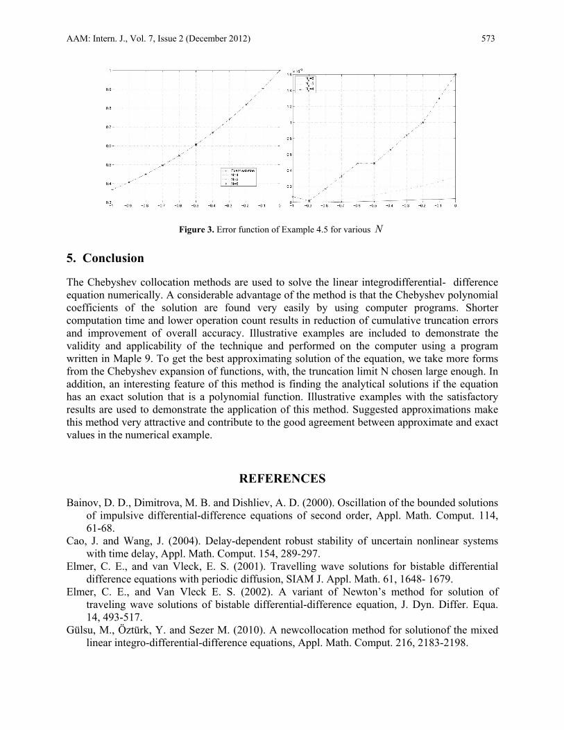
and its exact solution is xexy )( . We obtain the approximate solution of the problem for 4N , 5N , 6N which are tabulated and graphed in Table 3 and Figure 3 respectively.

Table 3: Numerical solution of Example 4.5 for different N



5. Conclusion The Chebyshev collocation methods are used to solve the linear integrodifferential- difference equation numerically. A considerable advantage of the method is that the Chebyshev polynomial coefficients of the solution are found very easily by using computer programs. Shorter computation time and lower operation count results in reduction of cumulative truncation errors and improvement of overall accuracy. Illustrative examples are included to demonstrate the validity and applicability of the technique and performed on the computer using a program written in Maple 9. To get the best approximating solution of the equation, we take more forms from the Chebyshev expansion of functions, with, the truncation limit N chosen large enough. In addition, an interesting feature of this method is finding the analytical solutions if the equation has an exact solution that is a polynomial function. Illustrative examples with the satisfactory results are used to demonstrate the application of this method. Suggested approximations make this method very attractive and contribute to the good agreement between approximate and exact values in the numerical example.

REFERENCES

Bainov, D. D., Dimitrova, M. B. and Dishliev, A. D. (2000). Oscillation of the bounded solutions of impulsive differential-difference equations of second order, Appl. Math. Comput. 114, 61-68.

Cao, J. and Wang, J. (2004). Delay-dependent robust stability of uncertain nonlinear systems with time delay, Appl. Math. Comput. 154, 289-297.

Elmer, C. E., and van Vleck, E. S. (2001). Travelling wave solutions for bistable differential difference equations with periodic diffusion, SIAM J. Appl. Math. 61, 1648- 1679.

Elmer, C. E., and Van Vleck E. S. (2002). A variant of Newton’s method for solution of traveling wave solutions of bistable differential-difference equation, J. Dyn. Differ. Equa. 14, 493-517.

Gülsu, M., Öztürk, Y. and Sezer M. (2010). A newcollocation method for solutionof the mixed linear integro-differential-difference equations, Appl. Math. Comput. 216, 2183-2198.


Hosseini, S. M. and Shahmorad, S. (2003). Numerical solution of a class of integrodifferential equations by the Tau method with an error estimation, Appl. Math. Comput. 136:559-570.

Kadalbajoo, M. K. and Sharma, K. K. (2002). Numerical analysis of boundary-value problems for singularly-perturbed differential-difference equations with small shifts of mixed type, J. Optim. Theory Appl. 115:145-163.

Kadalbajoo, M. K.and Sharma, K. K. (2004). Numerical analysis of singularly-perturbed delay differential equations with layer behavior, App. Math. Comput. 157:11-28.

Maleknejad, K. and Mirzaee, F. (2006). Numerical solution of integro-differential equations by using rationalized Haar functions method, Kybernetes Int. J. Syst. Math. 35:1735-1744.

Ortiz, E. L., and Aliabadi, M. H. (1998). Numerical treatment of moving and free boundaryvalue problems with the Tau method, Comp. Math. Appl. 35(8), 53- 61.

Rashed, M. T. (2004). Numerical solution of functional differential, integral and integro-differential equations, Appl. Numer. Math. 156, 485-492.

Ren, Y., Zhang, B. and Qiao, H. (1999). A simple Taylor-series expansion method for a class of second kind integral equations, J. Comp. Appl. Math. 110, 15-24.

Sezer, M. and Gulsu, M. (2005). Polynomial solution of the most general linear Fredhol integro-differential-difference equation by means of Taylor matrix method, Int. J. Complex Var. 50(5):367-382.

Sezer, M. and Gülsu, M. (2005). A new polynomial approach for solving difference and Fredholm integro-difference equations with mixed argument, Appl. Mat. Comp. 171, 332- 344.

Synder, M. A. (1966). Chebyshev methods in Numerical Approximation, Prentice Hall, Inc., London.

Zhao, J. and Corless, R. M. (2006). Compact finite difference method for integrodifferential equations, Appl. Math. Comput. 177:271-288.

Date post:	01-Jun-2020
Category:	Documents
Upload:	others
View:	6 times
Download:	0 times

On The Numerical Solution of Linear Fredholm-Volterra ...€¦ · Hence, the matrix representation...

Documents