50

On the pricing of Bermudanswaptions with an application tolimited observed market data
Mattias Jansson
Royal Institute of TechnologyLindstedts väg 13
SE-100 44 Stockholm, Sweden
Algorithmica Research ABHamngatan 13
SE-111 47 Stockholm, Sweden

.

Abstract
The focus of this thesis is on the risk neutral valuation of Bermudan swaptionsand its application to pricing situations where observed market data used forcalibration is limited. By exploring the properties of the solution to the optimalstopping problem that species the price process of these instruments, a generalvaluation method suited for practical computations is suggested. The valuationmethod is based on restricting the evolution of the short rate process to thatof a recombining binomial tree and is able to produce fast price estimates ofBermudan swaptions based on limited input data when specifying the dynamicsof the short rate process to the Ho-Lee model.

.

Acknowledgements
This master thesis has been conducted in collaboration with Algorithmica Re-search AB and I would like to take the opportunity to thank all members of thesta who have helped and supported me on the way to completing the work,especially my supervisor Peter Alaton who has provided me with much adviceon various aspects of the interest rate market.I would furthermore like to thank my supervisor at the Royal Institute of Tech-nology, Professor Boualem Djehiche, for all his encouragement and advice at allstages of the project.Last but not least, I want to acknowledge all encouragement and support givento me by my family and my girlfriend, Aurora, during this process.

.
Contents
1 Introduction 7
2 Preliminaries 92.1 Zero coupon bonds . . . . . . . . . . . . . . . . . . . . . . . . . . 92.2 The bank account . . . . . . . . . . . . . . . . . . . . . . . . . . 92.3 LIBOR spot rates . . . . . . . . . . . . . . . . . . . . . . . . . . . 102.4 Eective zero rates . . . . . . . . . . . . . . . . . . . . . . . . . . 11
3 Denition of instruments 123.1 The interest rate swap . . . . . . . . . . . . . . . . . . . . . . . . 12
3.1.1 The payer swap . . . . . . . . . . . . . . . . . . . . . . . . 123.2 The Bermudan swaption . . . . . . . . . . . . . . . . . . . . . . . 14
3.2.1 The Bermudan payer swaption . . . . . . . . . . . . . . . 15
4 Pricing Bermudan swaptions 174.1 Stopping times . . . . . . . . . . . . . . . . . . . . . . . . . . . . 18
4.1.1 Stopping times and Bermudan swaptions . . . . . . . . . 184.2 Derivation of an optimal stopping time . . . . . . . . . . . . . . . 19
5 Using the pricing envelope in practice 225.1 Introducing a new pricing envelope . . . . . . . . . . . . . . . . . 22
5.1.1 Interpretation of the envelope . . . . . . . . . . . . . . . . 24
5
5.1.2 Extension of the envelope . . . . . . . . . . . . . . . . . . 255.2 Pricing with a binomial tree . . . . . . . . . . . . . . . . . . . . . 26
5.2.1 Approximating the pricing procedure . . . . . . . . . . . . 285.2.2 The approximation error . . . . . . . . . . . . . . . . . . . 29
6 Pricing according to the Ho-Lee short rate model 306.1 The Ho-Lee short rate model . . . . . . . . . . . . . . . . . . . . 306.2 Pricing the Bermudan swaption . . . . . . . . . . . . . . . . . . . 326.3 Calibrating the model using limited data . . . . . . . . . . . . . . 336.4 Disadvantages of the model . . . . . . . . . . . . . . . . . . . . . 34
7 Numerical results 367.1 Convergence of the pricing procedure . . . . . . . . . . . . . . . . 377.2 Convergence of the calibration procedure . . . . . . . . . . . . . 387.3 Sensitivity measures . . . . . . . . . . . . . . . . . . . . . . . . . 39
7.3.1 Price sensitivity w.r.t. the short rate volatility . . . . . . 397.3.2 Price sensitivity w.r.t. the initial term structure . . . . . 40
8 Summary and conclusions 44
A Pricing zero coupon bonds using the Ho-Lee binomial tree 46

Chapter 1
Introduction
In recent years a lot of attention has been drawn to the problem of accuratelyand eectively pricing Bermudan swaptions. A number of pricing procedures,such as those described in [1], [3], [8], [9] and [10], have resulted from thisresearch. All these methods have a common property in that they require fairlyadvanced market data for calibration and furthermore employ computationallyintense procedures when calibrating. For a nancial institution, the complexityof these procedures is generally manageable, but for non-nancial corporateshaving positions in Bermudan swaptions, it may quickly become a hard problem.For these parties, gathering and processing the extensive collection of marketdata (such as prices for caps, oors and interest rate swaps) needed to make thepricing procedures work as well as performing and ne tuning the calculations,usually results in a time consuming, or at worst, an impossible task. As aconsequence of this, they are thus more or less left without a means to valueand assess the risk of their position.Assuming that these parties receive valuations from the counter party of theBermudan swaption on regular intervals and that they are able to access widelyquoted interest rate curves, there is however as will be revealed, a way for themto retrieve an estimate of the sought information.The purpose of this thesis is twofold. Firstly, the optimal stopping problem ofpricing the Bermudan swaption through risk neutral valuation will be studiedand solved as the optimum of a deterministic dynamic programming problem.Secondly, the properties of the derived solution will be explored in order tond a means to convert the theoretical results into a pricing procedure suit-able for practical purposes. A specialization of this method, adjusted to thepreviously described calibration circumstances, will then nally be proposed us-ing the Ho-Lee binomial tree representation of the short rate. Although, thismethod generally is considered to generate relatively crude results, it will pro-vide a quickly calculated estimate of the price of the Bermudan swaption to theparties lacking the possibility of using more complex models.
7

8 Chapter 1. Introduction
The remainder of this thesis is organized as follows. Chapter 2 gives a briefintroduction to the concepts used throughout the rest of this thesis when de-riving results regarding the pricing of Bermudan swaptions. Chapter 3 providesa denition of the interest rate swap as well as a denition of the Bermudanswaption and its price process. In Chapters 4 and 5 we derive and discuss thetheoretical solution to the pricing problem and study how these results may beused in practical pricing situations. In Chapter 6 we then study a special caseof the previously derived pricing procedure having a calibration procedure ad-justed to the aforementioned limitations in observed market data. This pricingmethod is obtained by modelling the evolution of the short rate according tothe Ho-Lee model in discrete time. Chapter 7 presents some numerical resultson the behaviour of the Ho-Lee pricing method as well as its calibration pro-cedure. Chapter 8 nally summarizes and discusses the material covered in thethesis and suggests topics that remain to be studied.

Chapter 2
Preliminaries
The purpose of this chapter is to give a brief introduction to the concepts aswell as the notation that will be used throughout the rest of this thesis. Theinterested reader is referred to [2] for a thorough treatment of the covered ma-terial.
2.1 Zero coupon bonds
The market we will be working with in subsequent chapters is a complete marketfree of arbitrage characterized by having zero coupon bonds as its only asset.On a complete and ltered probability space (Ω,F , (Ft)t≥0) these instrumentsare dened as follows.
Denition 1. A zero coupon bond with maturity T is a contract which at time
T pays one unit of currency to its holder. The price at time 0 ≤ t ≤ T of a zero
coupon bond maturing at time T is denoted by p(t, T ), where (p(t, T ) ∈ Ft)0≤t≤T
and p(t, t) = 1 for all t ≥ 0.
2.2 The bank account
Given the previously introduced bond market, we now construct a derived in-strument that will be frequently used in chapters to come. This instrumentrepresents an investment free of risk continuously growing according to an in-terest rate the short rate and is commonly referred to as the bank account.
9
10 Chapter 2. Preliminaries
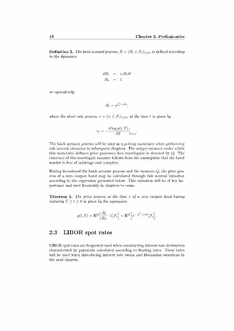
Denition 2. The bank account process, B = (Bt ∈ Ft)t≥0, is dened according
to the dynamics
dBt = rtBtdt
B0 = 1
or equivalently
Bt = e∫ t0 rsds,
where the short rate process, r = (rt ∈ Ft)t≥0, at the time t is given by
rt = −∂ log p(t, T )∂T
∣∣∣T=t
.
The bank account process will be used as a pricing numeraire when performingrisk neutral valuation in subsequent chapters. The unique measure under whichthis numeraire deates price processes into martingales is denoted by Q. Theexistence of this martingale measure follows from the assumption that the bondmarket is free of arbitrage and complete.Having introduced the bank account process and the measure Q, the price pro-cess of a zero coupon bond may be calculated through risk neutral valuationaccording to the expression presented below. This valuation will be of key im-portance and used frequently in chapters to come.
Theorem 1. The price process at the time t of a zero coupon bond having
maturity T ≥ t ≥ 0 is given by the expression
p(t, T ) = EQ[ Bt
BT· 1
∣∣Ft
]= EQ
[e−
∫ Tt
rsds∣∣Ft
].
2.3 LIBOR spot rates
LIBOR spot rates are frequently used when constructing interest rate derivativescharacterized by payments calculated according to oating rates. These rateswill be used when introducing interest rate swaps and Bermudan swaptions inthe next chapter.
2.4. Eective zero rates 11
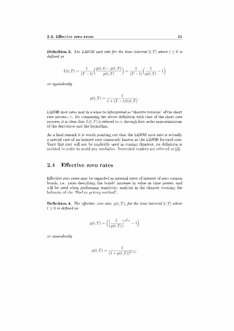
Denition 3. The LIBOR spot rate for the time interval [t, T ] where t ≥ 0 is
dened as
L(t, T ) =1
(T − t)
(p(t, t)− p(t, T )p(t, T )
)=
1(T − t)
( 1p(t, T )
− 1)
or equivalently
p(t, T ) =1
1 + (T − t)L(t, T ).
LIBOR spot rates may in a sense be interpreted as discrete versions of the shortrate process, r. By comparing the above denition with that of the short rateprocess, it is clear that L(t, T ) is related to rt through rst order approximationsof the derivative and the logarithm.As a nal remark it is worth pointing out that the LIBOR spot rate is actuallya special case of an interest rate commonly known as the LIBOR forward rate.Since this rate will not be explicitly used in coming chapters, its denition isomitted in order to avoid any confusion. Interested readers are referred to [3].
2.4 Eective zero rates
Eective zero rates may be regarded as internal rates of interest of zero couponbonds, i.e. rates describing the bonds' increase in value as time passes, andwill be used when performing sensitivity analysis in the chapter covering thebehavior of the Ho-Lee pricing method.
Denition 4. The eective zero rate, y(t, T ), for the time interval [t, T ] wheret ≥ 0 is dened as
y(t, T ) =([ 1
p(t, T )
] 1T−t − 1
)or equivalently
p(t, T ) =1
(1 + y(t, T ))T−t.

Chapter 3
Denition of instruments
In this chapter we dene the transactions and instruments studied in this the-sis and present expressions for their corresponding price processes. Althoughthe time structures used in the presentation are somewhat limited in order tomaintain manageable expressions, all derived results may easily be adjusted toa more general setup.
3.1 The interest rate swap
An interest rate swap, henceforth abbreviated as an IRS, is a contractual agree-ment between two parties under which each party agrees to make periodic in-terest payments to the other for an agreed period of time. The agreement inits most common form states that a series of payments calculated by applyinga xed rate of interest to a notional amount are exchanged for another seriesof payments calculated at the same notional amount using a oating rate ofinterest. The xed rate payment stream is traditionally called the xed leg,while the oating payments are referred to as the oating leg.Depending on whether a participant of an IRS agreement receives/pays the xedleg he is said to hold a receiver/payer swap. That is, the dierence between thetwo setups lies in the sign of the net ow of payments. As a consequence of this,once the price of one type of IRS is known, the price of the other is instantlyknown by reverting the sign of the rst price. Since the dierence in pricesindeed is minor, we only provide the derivation of the price of the payer swap.
3.1.1 The payer swap
Consider a xed set of equidistantly spaced dates T0, T1, . . . , TN such that δ =Ti − Ti−1 for all i = 1, 2, . . . , N . The payer swap is dened according to thefollowing agreement:
12

3.1. The interest rate swap 13
• All cash ows will be paid and received at the dates T1, T2, . . . , TN .• At the beginning of each period, [Ti−1, Ti], the LIBOR spot rate, L(Ti−1, Ti),is set and the amount κδL(Ti−1, Ti) is received by the holder at the date
Ti where i = 1, . . . , N . The amount κ is called the notional amount.• For the same period, [Ti−1, Ti], the holder pays the amount κδR, at thedate Ti where i = 1, . . . , N and R is constant. The rate at which thesepayments are made, R, is called the swap rate.
Using the above specics of the contract together with the denition of theLIBOR spot rate, the net cash ow of the payer swap at the date Ti can beexpressed as
κδ(L(Ti−1, Ti)−R
)= κ
( 1p(Ti−1, Ti)
− (1 + δR)). (3.1)
We now wish to determine the value of this net income, denoted Ni(t), at atime t ≤ T0, i.e. before the rst settlement date. Risk neutral valuation gives
Ni(t) = EQ[e− ∫ Ti
t rsdsκ(
1p(Ti−1,Ti)
− (1 + δR))∣∣∣Ft
]= κ
(EQ
[e− ∫ Tit rsds 1
p(Ti−1,Ti)
∣∣∣Ft
]− (1 + δR)p(t, Ti)
) (3.2)
where the cash ow κ(1 + δR) obviously may be interpreted as the face valueof a zero-coupon bond maturing at the date of the net transaction. In orderto price the rst term in the net income, we need to perform some furthercalculations. By conditioning the expectation on a larger σ-algebra, FTi−1 ⊇ Ft,and extracting the information stored therein we get
EQ[e− ∫ Ti
t rsds 1p(Ti−1,Ti)
∣∣Ft
]=
EQ[EQ
[e− ∫ Ti−1t rsdse−
∫ TiTi−1
rsds 1p(Ti−1,Ti)
∣∣FTi−1
]∣∣∣Ft
]=
EQ[e− ∫ Ti−1
t rsds 1p(Ti−1,Ti)
EQ[e− ∫ Ti
Ti−1rsds∣∣FTi−1
]∣∣∣Ft
]=
EQ[e− ∫ Ti−1
t rsds∣∣Ft
].
From the above calculation, it becomes clear that the rst term in the expressionfor the net cash ow, (3.2), is valued as κp(t, Ti−1) at the date t ≤ T0. Usingthis fact together with earlier calculations, we nally end up at the net incomevaluation
Ni(t) = κ(p(t, Ti−1)− (1 + δR)p(t, Ti)
). (3.3)
Determining the total value at the time t ≤ T0 of the payer swap, PS(t;κ, δ, R),now amounts to summing up all the values of the net incomes and thus we get

14 Chapter 3. Denition of instruments
PS(t;κ, δ, R) =N∑
i=1
Ni(t) = κN∑
i=1
(p(t, Ti−1)− (1 + δR)p(t, Ti)
)
which simplies to
PS(t;κ, δ, R) = κ(p(t, T0)− p(t, TN )− δR
N∑i=1
p(t, Ti)). (3.4)
A few remarks are in order. First of all, the valuation formula above is validonly at times prior to the rst settlement date, i.e. t ≤ T0. At later instants,the value of the IRS is determined by summing up the discounted values of allyet unsettled net cash ows. If for instance, T0 ≤ Tk−1 < t ≤ Tk ≤ TN , thevalue of the payer swap would equal
PS(t;κ, δ, R) = κ(p(t, Tk)− p(t, TN )− δR
N∑i=k+1
p(t, Ti)).
Secondly, the swap rate, R, is not to be mistaken for the par swap rate. Thepar swap rate, Rp(t), is the swap rate at which the price of the IRS equals zeroand is calculated using (3.4) as
Rp(t) =p(t, T0)− p(t, TN )
δN∑
i=1
p(t, Ti). (3.5)
Although, IRS contracts in practice are formulated to have an initial price ofzero, swap rates do not necessarily have to be calculated at par, i.e. whereR = Rp.
3.2 The Bermudan swaption
A swaption is an option on an IRS, i.e. an instrument providing its holder theright, but not the obligation, to enter an IRS at a pre-specied date in thefuture. As the name suggests, an option with the Bermudan characteristic, maybe considered as being situated somewhere in the gap between the Europeanoption having a single exercise date and the American option having acontinuous range of exercise dates in terms of its set of possible exercise dates.That is to say, a Bermudan swaption is a swaption having multiple discretelypositioned exercise dates.The following section provides a closer denition of the Bermudan swaptionin terms of its typical setup and risk neutral valuation. The focus will be on

3.2. The Bermudan swaption 15
swaptions having a payer swap as its underlying instrument. These types ofswaptions are henceforth referred to as payer swaptions.
3.2.1 The Bermudan payer swaption
Before getting into details about the exercise features of the Bermudan swaptionwe need to consider the underlying payer swap of the option. Using the setupand results described in the previous section we similarly dene this swap as:
• The underlying payer swap has N equidistantly spaced dates, T1, T2, . . . , TNwhere cash ows occur. The cash ows are identical to those described inthe previous section with the exception that the xed leg follows the swaprate Rs. This swap rate is called the swaption's strike rate.
• The value process of the swap at the time t ≤ TN−1 is PS(t;κ, δ, Rs).
There are several possible ways of constructing a Bermudan swaption when itcomes to deciding the setup of exercise dates. The arrangement that is used inthis thesis is basically the same as described in [3]:
• The swaption may be exercised at one of M + 1 number of xed exercisedates. These dates are denoted T e
i and all coincide with settlement datesof the underlying IRS, i.e. T e
i ∈ T0, T1, . . . , TN−1, i = 0, 1, . . . ,M .• The rst exercise date of the swaption equals1 the rst settlement date ofthe underlying IRS, i.e. T e
0 = T0.
Before continuing with the risk neutral valuation of the Bermudan swaptionwe need to determine the option's payo function. Unlike for instance optionson stock, swaptions, are not characterized by strike prices. Instead, swaptionsuse strike rates specifying the swap rate, R = Rs, of the underlying IRS of theoption. To make matters more specic, consider for instance the case whenthe swaption is exercised at the date T e
i for some i = 0, 1, . . . ,M . The payofunction generated as a consequence of the exercise is then given by
maxPS(T ei ;κ, δ, Rs), 0
.
As is clear from the payo function, one could claim that swaptions use strikeprices equalling zero. Remembering that market practice is to construct swapsusing par swap rates in order to achieve an initial value of zero, a possibleinterpretation of this choice of strike price is that the holder chooses to exercise
1This might seem like a limitation to generality at rst, but assuming that T e0 > T0 would
in fact be pointless since the holder of the swaption wouldn't be able to access any cash owssettled earlier than T e
0 , which in the context of pricing the swaption makes all settlement datesearlier than T e
0 redundant.

16 Chapter 3. Denition of instruments
the option only when the strike rate is suciently low compared to the par swaprate (the swap rate used for trading an identical swap on the market). In thatcase, the value of the payer swap would be positive implying that the owner ofthe swaption would make prot entering the IRS agreement.Having dened the underlying IRS and the exercise feature of the Bermudanswaption it is possible to calculate its price, BPS(T e
0 ;κ, δ, Rs), at the time T e0using risk neutral valuation as
BPS(T e0 ;κ, δ, Rs) = sup
τ∈SEQ
[ e− ∫ τT e0
rsds maxPS(τ ;κ, δ, Rs), 0∣∣FT e
0
] (3.6)
where the supremum is taken over the set, S, of all E-stopping times with valuesin the set T e
i , i = 0, 1, . . . ,M. The ltration E is dened as
E = (FT ei)Mi=0. (3.7)
The concept of stopping times will be dened and studied more closely in thenext chapter which has its focus on solving, i.e. nding the supremum of, theabove pricing problem. Until then, the reader may think of these variablesas exercise strategies adapted to the stochastic movements of the interest ratemarket, i.e. strategies deciding at which of the times T e
0 , T e1 , . . . , T e
M the optionshould be exercised.As a nal remark it is important to point out that although studying the pricingof Bermudan swaptions at the instant T e
0 might seem like a large limitation togenerality, retrieving the price at any time prior to the rst exercise date isin fact quite easily accomplished. The price at any instant t ≤ T e
0 is simplycalculated as the expectation of the discounted swaption valuation at T e
0 (cf.calculating the price of European options) and the reason we choose to focuson the valuation at the rst exercise date is only motivated by the fact that iteases up the notation and keeps focus on the essentials.
Chapter 4
Pricing Bermudan swaptions
In the previous chapter, the price at T e0 of a Bermudan payer swaption was
stated according to the risk neutral valuation expression
BPS(T e0 ;κ, δ, Rs) = sup
τ∈SEQ
[ e− ∫ τT e0
rsds maxPS(τ ;κ, δ, Rs), 0∣∣FT e
0
], (4.1)
where the supremum is taken over all E-stopping times. Though this expressionsure enough uniquely determines the price of the option, it cannot be evaluatedusing straightforward calculations since the price is determined as a solution toa stochastic optimization problem. This particular optimization problem is thefocus of this chapter where we introduce the concepts of stopping times andSnell envelopes and solve the above stated valuation problem.In order to ease up the notation when solving (4.1) the rest of this chapter isfocused on the treatment of the problem
V = supτ∈S0
EQ[fτ
∣∣F0
] (4.2)
where f = (fi ∈ Fi)Mi=0 is a stochastic process in discrete time and S0 belongs tothe set (Si)M
i=0 where Si denotes the set of all F i-stopping times. The ltrationF i is a member of the set (F i)M
i=0 specied by
F i = (Fk)Mk=i, i = 0, 1, . . . ,M.
The process f represents the discounted payo process of the Bermudan payerswaption and is assumed to be limited by the constraint
EQ [ |fi| ] < ∞, i = 0, 1, . . . ,M.
17

18 Chapter 4. Pricing Bermudan swaptions
As a nal remark its worth emphasizing that solving (4.1) by working with (4.2)not only simplies the notation but also generalizes the results somewhat. Eventhough the process f in this thesis is dened in the context of pricing Bermudanswaptions, the solution to the problem (4.2) is of course valid for any discretetime process limited by the above stated integrability constraint. In other words,by nding the optimal stopping time and the solution to this problem, we havein fact found the solution to the risk neutral valuation problem of any optionhaving a nite set of pointwise positioned exercise dates.
4.1 Stopping times
The solution to the pricing problem (4.2) is found by optimizing on a set ofstopping times. In order to nd the optimum we thus need to get a properunderstanding of these variables.Denition 5. A random variable, τ , taking values in i, i+1, . . . ,M is called
a F i-stopping time or a stopping time for the ltration F i if
τ ≤ k ∈ Fk, k = i, i + 1, . . . ,M
Stopping times are frequently used in the context of decision making underuncertainty, where they serve as variables determining when particular measuresare to be taken, e.g. when to leave a gambling table or when to exercise anoption having multiple exercise dates. By denition, a stopping time can onlydetermine whether a certain measure is to be taken at a time provided that theinformation generated up to that time is available. It can not with certaintyassume values corresponding to times yet to come based on what has happenedup to present time.
4.1.1 Stopping times and Bermudan swaptions
Knowing the denition of stopping times, a natural question to pose is whatmotivates the approach of pricing Bermudan swaptions (or any other derivatehaving an early exercise feature for that matter) using these variables. A keyobservation needed in order to answer that question, is that some way of rep-resenting a strategy determining when to exercise the option, needs to be es-tablished. As more money is assumed to be associated with higher utility thanless money for all actors in a derivates market according to arbitrage theory,this strategy should furthermore strive to maximize the payo received whenexercising the swaption.Bermudan swaptions are instruments traded on an interest rate market asso-ciated with uncertainty. As an exercise strategy should take the stochasticmovements of this market into consideration a reasonable model of this strat-egy would be through the use of random variables. Furthermore, the strategy

4.2. Derivation of an optimal stopping time 19
should have the property that an exercise decision should be made based on allinformation generated by the market up to that point in time. There would, forinstance, be no point in deciding to exercise the swaption in a year from now,as that decision should needless to say be made then, not now. Taking thesemodel demands into account together with the previous discussion on choosingan exercise strategy maximizing the received payo, the reason why Bermudanswaptions are priced as optimal stopping problems is motivated. The propertiesof an exercise strategy coincide with those of a stopping time and the task ofobtaining a price for the Bermudan swaption becomes equivalent with nding astrategy that maximizes the expectation of the discounted payo of the option.
4.2 Derivation of an optimal stopping time
We now turn to the problem of nding an optimal stopping for the pricingproblem (4.2) and begin by introducing the stochastic process v = (vi ∈ Fi)M
i=0given by
vM = fM
vi = max fi , EQ[vi+1
∣∣Fi
], i = 0, 1, . . . ,M − 1.
(4.3)
Using this process we furthermore introduce the F i-stopping times θi ∈ Si fori = 0, 1, . . . ,M dened by
θi = mink = i, i + 1, . . . ,M : fk = vk
, i = 0, 1, . . . ,M. (4.4)
The process, v, is commonly referred to as a Snell envelope for the stochasticprocess f and plays an important role in the problem of pricing Bermudanswaptions as will be revealed shortly. Before reaching this result however, weneed to make an important observation.
Lemma 1. For i = 0, 1, . . . ,M , the process v satises the relation
vi = EQ[fθi
∣∣Fi
]≥ EQ
[fτ
∣∣Fi
], τ ∈ Si.
Proof. The proof is given by an inductive argument. We begin by noting thatthe relation by denition is satised with equality for i = M and furthermoremake the assumption that the relation is valid for the times i = M,M−1, . . . , k.Showing that this assumption implies that the relation is valid for k − 1 thenconcludes the proof.Letting τ ∈ Sk−1 be an arbitrary Fk−1-stopping time and introducing τ ∈ Sksuch that τ = maxτ, k we make the following observation for some eventA ∈ Fk−1

20 Chapter 4. Pricing Bermudan swaptions
EQ[1Afτ
]= EQ
[1A∩τ=k−1fτ
]+ EQ
[1A∩τ≥kfτ
]= EQ
[1A∩τ=k−1fk−1
]+ EQ
[EQ
[1A∩τ≥kfτ
∣∣Fk−1
]]= EQ
[1A∩τ=k−1fk−1
]+ EQ
[EQ
[1A∩τ≥kfτ
∣∣Fk−1
]].
Since τ = k − 1 ∈ Fk−1, conditioning on a smaller σ-algebra implies that
EQ[1Afτ
]= EQ
[1A∩τ=k−1fk−1
]+ EQ
[1A∩τ≥kEQ
[fτ
∣∣Fk−1
]]= EQ
[1A∩τ=k−1fk−1
]+ EQ
[1A∩τ≥kEQ
[EQ[ fτ |Fk]
∣∣Fk−1
]]≤ EQ
[1A∩τ=k−1fk−1
]+ EQ
[1A∩τ≥kEQ
[vk
∣∣Fk−1
]]≤ EQ
[1Avk−1
]where the second last inequality follows from the induction hypothesis and thelast inequality is an immediate consequence of the denition of the Snell enve-lope. As the above inequality is valid for all events A ∈ Fk−1, conditioning theabove expectations on Fk−1 necessarily results in
vk−1 ≥ EQ[fτ
∣∣Fk−1
]which proves the inequality relation stated in the lemma. It remains to verifythat this inequality is satised with equality for the Fk−1-stopping time θk−1.Returning to the chain of inequalities above, we conclude that
EQ[1Afθk−1
]= EQ
[1A∩θk−1=k−1fk−1
]+ EQ
[1A∩θk−1≥kEQ
[vk
∣∣Fk−1
]].
as a consequence of the induction hypothesis. Furthermore the equality relation
EQ[1A∩θk−1=k−1fk−1
]+ EQ
[1A∩θk−1≥kEQ
[vk
∣∣Fk−1
]]= EQ
[1Avk−1
]must necessarily hold since vk−1 = fk−1 for the event θk−1 = k−1 and vk−1 =EQ[vk|Fk−1] for the complementary event θk−1 ≥ k where vk−1 6= fk−1. Asa nal consequence, conditioning the expectation on Fk−1 and using the factthat the above relation holds for all events A ∈ Fk−1 results in

4.2. Derivation of an optimal stopping time 21
vk−1 = EQ[fθk−1
∣∣Fk−1
]which completes the proof.
Using this lemma we can now construct an optimal stopping time for the prob-lem (4.2) and thereby obtain an explicit expression for the price process of theBermudan swaption in terms of the Snell envelope, v.
Theorem 2. The price process, V , satises the relation
V = EQ[fθ0
∣∣F0
]= v0
where v0 is determined by the recursion
vM = fM
vi = max
fi , EQ[vi+1
∣∣Fi
], i = 0, 1, . . . ,M − 1.
and the optimal F0-stopping time θ0 is given by
θ0 = min
k = 0, 1, . . . ,M : fk = vk
.
Proof. The proof follows from Lemma 1 since
v0 = EQ[fθ0
∣∣F0
]≥ EQ
[fτ
∣∣F0
], τ ∈ S0.
together with the denition of V implies that
V = supτ∈S0
EQ[fτ
∣∣F0
]= EQ
[fθ0
∣∣F0
]= v0.
The theorem above provides an optimal stopping time for the problem (4.2)and states the solution of the problem as a Snell envelope for the process f . Inthe next chapter we discuss how this solution can be used in practice to priceBermudan swaptions.

Chapter 5
Using the pricing envelope in
practice
According to the theorem presented in the previous chapter, a Bermudan swap-tion could be priced through a back stepping method, i.e. a method where theprice V = v0 is calculated by iteratively constructing the process v in descend-ing order of time. A problem with this procedure is that it typically results incomplex and time consuming computations, since it relies on calculating chainsof expected values represented by multidimensional integrals. Calculating theseintegrals using numerical methods is known to be a notoriously cumbersometask (see [6] for further discussion).In order to avoid this problem a simplied pricing method based on using dis-crete approximations of the continuous processes v and f is commonly used inpractice. The discrete approximations are obtained by restricting the evolutionof the stochastic processes to tree structures, which only allow each process toevolve to one of a nite number of states at a given point in time. When applyingthese approximations, the above discussed continuous integrals are transformedto ordinary sums which considerably lowers the complexity of the calculations.The focus of this chapter is to study how one of these tree methods can beused to price Bermudan swaptions by restricting the evolution of the short rateprocess to that of a recombining binomial tree.
5.1 Introducing a new pricing envelope
Using the results presented in the previous chapter together with an adjustmentof the set of admissible exercise dates, the initial price of a Bermudan swaptionis given as
22

5.1. Introducing a new pricing envelope 23
BPS(T e0 ;κ, δ, Rs) = v0
where v is redened as
vi = maxfi,EQ[vi+1
∣∣FT ei
], i = 0, 1, . . . ,M − 1
vM = fM
and the process f is identied as
fi = e−∫ T e
iT e0
rsds maxPS(T ei ;κ, δ, Rs), 0
, i = 0, 1, . . . ,M.
We now introduce the envelope u = (ui ∈ FT ei)Mi=0 given by
ui = maxFi,EQ[ e− ∫ T e
i+1T e
irsds
ui+1
∣∣FT ei
], i = 0, 1, . . . ,M − 1
uM = FM
(5.1)
where the process F = (Fi ∈ FT ei)Mi=0 is dened by
Fi = maxPS(T ei ;κ, δ, Rs), 0
, i = 0, 1, . . . ,M. (5.2)
In order to be able to introduce the binomial tree pricing method as it is typicallyused in practice (see [3]), we will abandon the pricing of Bermudan swaptionsthrough the use of the process v in favour of the process u. The followingtheorem veries the legality of this alternative pricing method.Theorem 3. The initial price of the Bermudan swaption is given by the pro-
cesses u and F dened by (5.1) and (5.2) as
BPS(T e0 ;κ, δ, Rs) = u0.
Proof. The proof is constructed by an induction argument verifying the relation
vi = uie−∫ T e
iT e0
rsds, i = 0, 1, . . . ,M
which implies that the new pricing method is valid since v0 = u0. We be-gin by concluding that the relation by denition of f and F is true at thetime T e
M and furthermore make the assumption that the relation holds for

24 Chapter 5. Using the pricing envelope in practice
T eM , T e
M−1, . . . , Tek+1 for some k = 0, 1, . . . ,M − 2. This assumption however
implies that the relation is valid at T ek since
vk = maxfk,EQ[vk+1
∣∣FT ek
]= maxe− ∫ T e
kT e0
rsdsFk,EQ
[uk+1e−
∫ T ek+1
T e0
rsds∣∣FT ek
]= maxe− ∫ T e
kT e0
rsdsFk,EQ
[uk+1e−
∫ T ek
T e0
rsds−∫ T e
k+1T e
krsds∣∣FT e
k
]= e−
∫ T ek
T e0
rsdsmaxFk,EQ[uk+1e−
∫ T ek+1
T ek
rsds∣∣FT ek
]= uke−
∫ T ek
T e0
rsds
which proves the induction hypothesis and thereby the theorem.
5.1.1 Interpretation of the envelope
As was previously stated, the price of a Bermudan swaption may be retrievedusing the envelope u through the relation BPS(T e
0 ;κ, δ, Rs) = u0 where
u0 = maxF0,EQ[ e− ∫ T e
1T e0
rsdsu1
∣∣FT e0
]u1 = maxF1,EQ
[ e− ∫ T e2
T e1
rsdsu2
∣∣FT e1
]...
uM−1 = maxFM−1,EQ[ e− ∫ T e
MT e
M−1rsds
uM
∣∣FT eM
]uM = FM
According to this recursion, we may interpret the calculation of the initial priceof the swaption, u0, as nding the maximum value of either exercising the optionimmediately and thereby receiving the payo F0, or postponing the exercisedecision until later. The value of choosing not to exercise the option at T e
0 isaccording to the above relations calculated as the discounted initial value of aBermudan swaption having its rst exercise date at T e
1 . The initial value of thisoption, u1, is correspondingly calculated using the same procedure as for u0, i.e.by comparing which of the alternatives exercising immediately or postponingthe exercise decision that is associated with the highest expected value.By repeating this pricing procedure until reaching the last exercise date, T e
M , theprice of the Bermudan swaption is obtained through a dynamic programmingrelation. The value of uM , representing the initial (initial meaning the time T e
M )price of a swaption having its rst and only exercise date at T e
M , must necessarily

5.1. Introducing a new pricing envelope 25
satisfy the equality uM = FM , i.e. the initial price of the option equals the valueof its immediate payo. Since uM can be calculated explicitly, the sequenceuM−1, uM−2, . . . , u0 may be calculated as well in an iterative fashion.Pricing Bermudan swaptions using the process u could be argued to be moreintuitive than the pricing procedure based on the envelope v. Sure enough,both methods are identical in the sense that they render the same valuation bycomparing which of the alternatives immediate exercise or postponed exer-cise that is more protable. What separates them, however, is the way thesealternatives are quantied. When using the original pricing method based onthe processes v and f , the comparison is always done by discounting all val-ues to the time T e
0 . The new method, on the other hand, always performs thediscounting to the time of the comparison, which might be considered as moreappealing from an intuitive point of view.
5.1.2 Extension of the envelope
It will prove useful to know the value of the process u at all settlement datesbetween the rst and the last exercise date1 of the Bermudan swaption. For thisreason, the envelope is extended to be dened on these dates in this section. Asa rst step in doing so, we begin by dening the index K (cf. gure 5.1 below)as
K =l = 1, 2, . . . , N : Tl = T e
M
(5.3)
and redene the process u as u = (ui ∈ FTi)Ki=0. In order to calculate the value
of this envelope at a certain time, we furthermore need to establish a meansto identify if this time corresponds to an exercise date or not, as ui necessarilymust be valued dierently than (5.1) at non-exercise dates. This is achieved byintroducing the indicators Ei dened by
Ei = 1Ti∈T e
0 ,T e1 ,...,T e
M, i = 0, 1, . . . ,K. (5.4)
When Ei = 1, the date Ti corresponds to an exercise date and ui is calculatedin the same manner as before the extension, i.e. through equation (5.1). Inthe opposite case when Ei = 0, the variable ui however represents the priceof a Bermudan swaption having its rst exercise date at a later instant thanTi, and should be calculated as the value of (necessarily) keeping the swaptionuntil at least the time Ti+1. This value is obtained by excluding the alternativeimmediate exercise in expression (5.1), i.e.
ui = EQ[ e− ∫ Ti+1
Tirsds
ui+1
∣∣FTi
], Ei = 0
1Recall from the denition in the previous chapter that the exercise dates are assumed tocoincide with settlement dates of the underlying IRS.

26 Chapter 5. Using the pricing envelope in practice
T0
T0e
T1
T2
T3
T1e
T4
T5
TN−2
TN−1
T2e . . . T
Me
TK . . . . . .
Exercise dates
Settlement dates
Figure 5.1: Example of a set of exercise dates of the Bermudan swaption togetherwith its underlying IRS's set of settlement dates. Note that the settlement dateTK is dened as the last exercise date of the swaption, i.e. TK = T e
M .
Using this result, the extended process u is completely specied as
ui =
maxFi,EQ[ e− ∫ Ti+1
Tirsds
ui+1
∣∣FTi
], Ei = 1
EQ[ e− ∫ Ti+1
Tirsds
ui+1
∣∣FTi
], Ei = 0
uK = FK
(5.5)
where the index i is dened on the set i = 0, 1, . . . ,K and the process F isextended to F = (Fi ∈ FTi
)Ki=0 and dened as
Fi = maxPS(Ti;κ, δ, Rs), 0
, i = 0, 1, . . . ,K. (5.6)
As before, the price of the Bermudan swaption is given by the value of theenvelope at the time T e
0 = T0, i.e. as
BPS(T e0 ;κ, δ, Rs) = u0. (5.7)
5.2 Pricing with a binomial tree
The approximate pricing method that is the focus of this chapter is based onrestricting the evolution of the short rate process to that of a recombining bi-nomial tree. In the following section we provide a closer examination on howthis discretization aects the extended pricing procedure (5.5)-(5.6).In order to make matters more specic, the short rate process, r, is replacedwith the nite state process r = (ri ∈ FTi)
N−1i=0 . Furthermore the notation ri,jis introduced, having the interpretation that the process on the time interval
[Ti, Ti+1) is in the state j, i.e. the value of ri is determined by the index j.Unlike all stochastic processes dened up to this point, r is dened on the setof dates (Ti)N−1
i=0 , where the index N − 1 denotes the ordinal number of the last
5.2. Pricing with a binomial tree 27
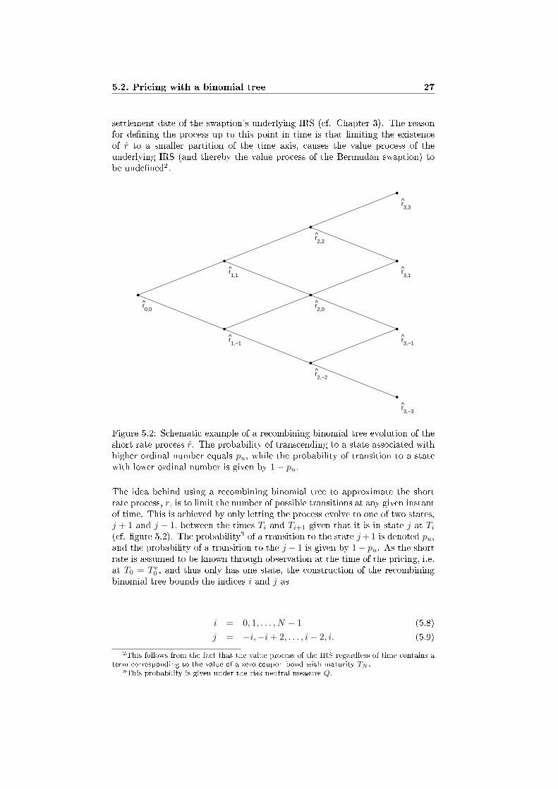
settlement date of the swaption's underlying IRS (cf. Chapter 3). The reasonfor dening the process up to this point in time is that limiting the existenceof r to a smaller partition of the time axis, causes the value process of theunderlying IRS (and thereby the value process of the Bermudan swaption) tobe undened2.
r0,0
^
r1,1
^
r2,2
^
r3,3
^
r1,−1
^
r2,−2
^
r3,−3
^
r2,0
^
r3,1
^
r3,−1
^
Figure 5.2: Schematic example of a recombining binomial tree evolution of theshort rate process r. The probability of transcending to a state associated withhigher ordinal number equals pu, while the probability of transition to a statewith lower ordinal number is given by 1− pu.The idea behind using a recombining binomial tree to approximate the shortrate process, r, is to limit the number of possible transitions at any given instantof time. This is achieved by only letting the process evolve to one of two states,j + 1 and j − 1, between the times Ti and Ti+1 given that it is in state j at Ti(cf. gure 5.2). The probability3 of a transition to the state j +1 is denoted pu,and the probability of a transition to the j − 1 is given by 1− pu. As the shortrate is assumed to be known through observation at the time of the pricing, i.e.at T0 = T e
0 , and thus only has one state, the construction of the recombiningbinomial tree bounds the indices i and j as
i = 0, 1, . . . , N − 1 (5.8)j = −i,−i + 2, . . . , i− 2, i. (5.9)
2This follows from the fact that the value process of the IRS regardless of time contains aterm corresponding to the value of a zero coupon bond with maturity TN .
3This probability is given under the risk neutral measure Q.

28 Chapter 5. Using the pricing envelope in practice
5.2.1 Approximating the pricing procedure
We now turn to the question of how the processes u and F are approximatedwhen restricting the evolution of the short rate process to that of a recombiningbinomial tree. As F by denition is given by
Fi = maxPS(Ti;κ, δ, Rs), 0
, i = 0, 1, . . . ,K
the short rate discretization must necessarily cause an approximation, since thevalue process PS(T e
i ;κ, δ, Rs) according to (3.4) is constructed as a sum of shortrate dependent zero coupon bonds with varying maturities. In order to furtherinvestigate the properties of this approximation, we thus need to nd out howthe price process of a zero coupon bond is approximated as a consequence ofintroducing the binomial tree. As this task typically generates a somewhatmessy notation unless the process r is further specied, we postpone the detailsof this calculation to the next chapter. Until then, we settle with introducingthe process F = (Fi ∈ FTi
)Ki=0 as the approximation of F leaving all details
aside. As in the case with the approximated short rate process, Fi,j denotesthat the process F is in the state j on the interval [Ti, Ti+1), where j is boundedby (5.9).It remains to investigate what eect the binomial tree has on the envelope udened as
ui =
maxFi,EQ[ e− ∫ Ti+1
Tirsds
ui+1
∣∣FTi
], Ei = 1
EQ[ e− ∫ Ti+1
Tirsds
ui+1
∣∣FTi
], Ei = 0
uK = FK
where i = 0, 1, . . . ,K. As was pointed out earlier, the reason for introducing anapproximate pricing method based on a binomial tree is motivated by the factthat the process u is partly constructed from an expectation of a continuousrandom variable. In order to deduce the simplications induced by this tree,we introduce the process u = (ui ∈ FTi
)Ki=0 approximating u, and furthermore
let ui,j denote that the value of ui is given by the state index j on the interval[Ti, Ti+1).By observing the above expression for u, it stands clear that we need to decideon how the stochastic integral over the short rate process (the discount factor) isvalued before approximating the aforementioned expected value. This however,turns out to be a relatively easy task since the approximated short rate process rby denition is constant over the period [Ti, Ti+1) at any given state j, meaningthat the integral reasonably should be discretized as
e(Ti+1−Ti)ri ∈ FTi.
5.2. Pricing with a binomial tree 29
Using this approximation, the process u should then suitably discretize u at allinstants of time and states as
ui,j =
maxFi,j , e(Ti+1−Ti)ri,j(puui+1,j+1 + (1− pu)ui+1,j−1
), Ei = 1
e(Ti+1−Ti)ri,j(puui+1,j+1 + (1− pu)ui+1,j−1
), Ei = 0
uK,j = FK,j (5.10)where the indices i and j are bounded by equations (5.8)-(5.9). Besides relyingupon the previously stated discretization of the discount factor, this approxima-tion uses the fact that restricting the short rate evolution to that of a recombin-ing binomial tree implies that the expectation could be discretely approximatedby a weighted sum. This sum consists of the terms ui+1,j+1 and ui+1,j−1 rep-resenting the two possible states the process u may transcend to at the timeTi+1.
5.2.2 The approximation error
Pricing Bermudan swaptions using a recombining binomial tree (or any othertree structure for that matter) naturally generates a valuation error as a conse-quence of limiting the evolution of all involved processes to a nite set of states.The magnitude of this error does however not only depend on the number ofstates each process is restricted to. A large contribution of the error is in factdue to the neness of the mesh on which the approximated short rate processis dened, since this process is assumed to be constant on every interval onthe mesh. Even though, we have dened the process r to exist only on thesettlement dates of the Bermudan swaption's underlying IRS throughout thischapter, this particular partition is in no way the only alternative available whenconstructing r. As a matter of fact, any mesh having equidistant4 nodes will doas long as it reaches as far as to the settlement date of the last transaction ofthe IRS, i.e. the time TN−1. The choice of introducing the approximate pricingmethod based on a mesh consisting solely of settlement dates, is only motivatedby the fact that it eases up the notation and keeps the focus on the essentialsteps of the method. Though this partition will be used in the next chapter aswell for the same reasons, the reader is advised to employ a ner mesh whenusing the method in practical situations.As a nal comment, it's worth pointing out that choosing to rene the mesh onwhich the process r is constructed, not only limits the pricing error due to thediscretization of the time axis. By increasing the number of nodes, the numberof states represented in the binomial tree multiplies. This causes a reduction inthe error induced by the restriction set on the evolution of the process as well.
4In order to produce a binomial tree with the property of being recombining, all points onwhich the approximated short rate process is dened, need to be equidistantly spaced.
Chapter 6
Pricing according to the
Ho-Lee short rate model
The purpose of this chapter is to make the previously introduced approximatepricing method explicit by specifying a model of the short rate process. Themodel in question was suggested in the seminal article [7] and has since thenbecome widely celebrated as it due to its parameterization, was the rst modelof the short rate guaranteeing absence of arbitrage.Besides introducing the Ho-Lee model and presenting its valuation of Bermudanswaptions, this chapter furthermore presents a way of calibrating the parametersof the model given limited observed market data as discussed in the introductionof this thesis. Despite the fact that the Ho-Lee model was introduced some 20years ago and lack many desirable features of today's short rate models (see [3]for a survey), it still is a competitive alternative when dealing with situationssuch as these due to the simplicity of its construction.
6.1 The Ho-Lee short rate model
When reading about the Ho-Lee model in recent literature on nancial math-ematics, the short rate process is usually presented having continuous timedynamics. In the original setup presented by the authors, the dynamics weredierent however, as the short rate process was dened in a discrete setting andhaving an evolution given by a recombining binomial tree. As the previouslyproposed approximate pricing method is constructed through the use of a bi-nomial tree, the model used in this chapter will be constructed similarly to theoriginal Ho-Lee model.Using the same notation and partition of the time axis as in the previous chapter,the short rate process in discrete time, r = (ri ∈ FTi
)N−1i=0 , is dened according
to the Q-dynamics
30

6.1. The Ho-Lee short rate model 31
ri = θi +√
δσ2
i∑k=1
BQk , i = 0, 1, . . . , N − 1 (6.1)
where δ (cf. Chapter 3) represents the equidistant time period between twosettlement dates of the underlying IRS of the Bermudan swaption and (BQ
k )N−1k=1is a stochastic sequence consisting of IID symmetric Bernoulli random variables
under the measure Q, i.e.
Q(BQk = +1) = 1/2,
Q(BQk = −1) = 1/2,
k = 1, 2, . . . , N − 1. (6.2)
In the above denition, the volatility, σ, of short rate process is dened as astrictly positive deterministic constant, i.e. σ > 0, while the drift of the process,(θi)N−1
i=0 , is dened as a deterministic sequence on R.
Figure 6.1: Example of the Ho-Lee short rate evolution in a binomial tree.Using the denition (6.1), the construction (cf. gure 6.1 for a typical example)of the process r implies that ri,j is given by
ri,j = θi + j√
δσ2,i = 0, 1, . . . , N − 1j = −i,−i + 2, . . . , i− 2, i
(6.3)
where ri,j as earlier denotes the value of the short rate process at time Ti whenits state is given by the index j. We may furthermore observe that the Ho-Lee

32 Chapter 6. Pricing according to the Ho-Lee short rate model
model through its use of symmetric Bernoulli distributed variables, species thetransition probability from state j to state j + 1 (and j − 1 for that matter) aspu = 1/2 regardless of the time of the transition.
6.2 Pricing the Bermudan swaption
Given the short rate model (6.1) we are now able to explicitly specify the pricingprocedure of Bermudan swaptions according to the method introduced in theprevious chapter. Using the same notation as earlier together with the abovedenitions of ri,j and pu the approximate envelope u is calculated as
ui,j =
maxFi,j ,12 eδθi+jσδ3/2 (
ui+1,j+1 + ui+1,j−1
), Ei = 1
12 eδθi+jσδ3/2 (
ui+1,j+1 + ui+1,j−1
), Ei = 0
uK,j = FK,j (6.4)where the indices i, j and K are dened as
i = 0, 1, . . . ,Kj = −i,−i + 2, . . . , i− 2, i
K =
l = 1, 2, . . . , N : Tl = T eM
.
(6.5)
Since the process F up to this point has not been dened, the above pricingexpression is yet to be complete. As was discussed previously, specifying thisprocess requires the calculation of the price of zero coupon bonds, which upuntil now has been postponed. Having parameterized the short rate model,this can however be with more ease and we begin by introducing the processpm = (pm
i ∈ FTi)Ni=0 denoting the approximated value process at time Ti of azero coupon bond having maturity Tm, where
i ≤ m, i,m = 0, 1, . . . , N. (6.6)
Using the same convention as for the process r, the variable pmi,j denotes that
the price process at time Ti of the zero coupon bond has a value correspondingto the state j. As a consequence of having specied the process r, the valueof pm
i,j is calculated as (the interested reader is referred to the derivation in theappendix)
pmi,j = e−δ
m−1∑k=i
θk−δ3/2σj(m−i)m−1∏
k=i+1
cosh(δ3/2σ(m− k)
) (6.7)

6.3. Calibrating the model using limited data 33
which using the expression for the price process of the underlying IRS of theBermudan swaption as described by equation (3.4) determines F as
Fi,j = maxκ(pi
i,j − pNi,j − δRs
N∑k=i+1
pki,j
), 0
Simplifying the above expression somewhat nally results in
Fi,j = maxκ(1− pN
i,j − δRs
N∑k=i+1
pki,j
), 0
(6.8)
which completely species the process u and thereby the price of the Bermudanswaption as
BPS(T e0 ;κ, δ, Rs) = u0,0 (6.9)
with u and F constructed using relations (6.4)-(6.8).
6.3 Calibrating the model using limited data
As was stated in the introduction to this chapter, the Ho-Lee short rate modelmay be calibrated using relatively simple and easily accessible market data. Inthis section we aim to motivate this assertion by assign values to all parametersof the model using only:
• The initial term structure, i.e. the curve p? =p?(T0, T ) : T ≥ T0
observed on the market.
• A counter party's valuation at T e0 = T0 of the Bermudan swaption, i.e.
the price BPS?.
We begin by determining what role the initial term structure plays in the cali-bration procedure. Using relation (6.7), the initial price of a zero coupon bondhaving maturity Tm is given by
pm0,0 = e−δ
m−1∑k=0
θkm−1∏k=1
cosh(δ3/2σ(m− k)
)
where we have made use of the fact that the only possible state of the short rateprocess r at T0 is given by j = 0. By forming the quotient of this price at twoconsecutive maturity dates, Tk and Tk+1, we furthermore observe that
34 Chapter 6. Pricing according to the Ho-Lee short rate model
pk+10,0
pk0,0
= e−δθkcosh(kσδ3/2
).
Rearranging the terms in this relation and inserting prices stored in the observedinitial term structure, results in that the sequence of drift parameters, (θi)N−1
i=0 ,reasonably should be estimated as
θesti =
1δ
[log
(p?(T0, Ti)
p?(T0, Ti+1)
)+ log
(cosh(iσestδ3/2
))], (6.10)
where (θesti )N−1
i=0 denotes the estimation of the sequence (θi)N−1i=0 and σest denotes
the estimation of the volatility of the short rate process. In order to be able tobe able to use this expression we obviously need a way of calculating σest. Thistask is however quite easily dealt with using the given valuation of the Bermudanswaption as this price implicitly determines the volatility as the solution to thenon-linear equation
BPS(T e
0 ;κ, δ, Rs, σest,
(θest
i (σest))N−1
i=0
)= BPS? (6.11)
which expresses the drift of the short rate process using relation (6.10) thusleaving σest as the only unknown parameter. This equation is quite easily solvedusing a numerical procedure, for instance the secant method (see the descriptionin [6]). As σ typically lies somewhere in the range of 0.5 · 10−2 to 1 · 10−2 inmost interest rate markets, qualied starting values for a numerical solver couldbe extracted from this interval.Solving equations (6.10)-(6.11) completely determines all parameters of theshort rate model based on the limited input data. As the drift of the short rateprocess is calculated so as to accurately reproduce the initial term structure,the short rate model obtained using the above presented calibration procedure,is furthermore guaranteed to be absent of arbitrage possibilities1.
6.4 Disadvantages of the model
Unlike many of the short rate models introduced in the last decade, the Ho-Leemodel lacks a property that is commonly referred to as mean reversion. Thisproperty guarantees that the short rate process constantly evolves towards atime varying equilibrium and signicantly reduces the probability of the eventthat the process becomes negative or grows unreasonably large. As the Ho-Lee
1This statement is on a ner note actually only partly true as only the prices that areactually used in the calibration procedure are correctly represented by the short rate model.All other prices will only be reproduced approximately. In order to reduce the approximationerror the short rate process needs to be dened on a ner partition of the time axis (cf. thediscussion in the previous chapter).

6.4. Disadvantages of the model 35
model lacks mean reversion it thus, in comparison to more recent short ratemodels, has a relatively high probability of exploding or turning negative atsome point in time.Another disadvantage of the Ho-Lee model follows from the fact that it assumesthat the volatility of the short rate is constant in time as well as determinis-tic. Several studies (see [3] and references therein) have shown that volatilityparameterizations such as these are over-simplistic and unable to for instancehandle notorious problems such as volatility smiles.

Chapter 7
Numerical results
In the following chapter we study the behaviour of the pricing method proposedin the previous chapter in terms of its convergence, calibration to market dataand sensitivity to changes in parameter values. Two Bermudan payer swaptionsserve as the basis for our conclusions, the rst one having an underlying IRS withits last transaction in 5 years (referred to as the 5 year contract) and the secondone having an underlying IRS with its last transaction in 10 years (referredto as the 10 year contract). As was pointed out in chapter 3, the presenteddenitions of IRS agreements and Bermudan swaptions were not given in theirmost general (or for that matter common) form. In order to construct the twoswaptions studied in this chapter according to typical market practice, we thusdeviate from our earlier framework somewhat. More specically, we allow theunderlying IRS contracts of both options to make oating rate payments fourtimes a year and xed rate payments once a year. Furthermore, both swaptionsmay only be exercised once a year, namely a couple of days before the xedleg settles. Dening the two Bermudan swaptions according to these criterions,obviously calls for an extension of the results derived up to this point. Thisextension may however be performed with relative ease since the fundamentalproperties of the pricing procedure still apply. All that needs to be reformulatedis the set of dates on which the pricing envelope and short rate process aredened.All pricing and calibration is performed on the rst exercise date of the twooptions. The strike rates of the options are calculated as the par swap ratesat the same date (Rs = 3.475% for the 5 year swaption and Rs = 4.120% forthe 10 year swaption). Finally, the curve containing the initial term structureused for obtaining the short rate drift process, (θest
i )N−1i=0 , as described in the
previous chapter was calculated implicitly using market prices of Swedish IRScontracts and a bootstrapping technique (see [3] for an introduction).
36
7.1. Convergence of the pricing procedure 37
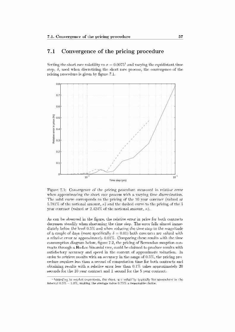
7.1 Convergence of the pricing procedure
Setting the short rate volatility to σ = 0.00751 and varying the equidistant timestep, δ, used when discretizing the short rate process, the convergence of thepricing procedure is given by gure 7.1.
10−2
10−1
0
0.1
0.2
0.3
0.4
0.5
0.6
0.7
0.8
Time step (yrs)
Rel
ativ
e er
ror
in p
rice
(%)
Figure 7.1: Convergence of the pricing procedure measured in relative errorwhen approximating the short rate process with a varying time discretization.The solid curve corresponds to the pricing of the 10 year contract (valued at5.781% of the notional amount, κ) and the dashed curve to the pricing of the 5year contract (valued at 2.424% of the notional amount, κ).As can be observed in the gure, the relative error in price for both contractsdecreases steadily when shortening the time step. The error falls almost imme-diately below the level 0.5% and when reducing the time step to the magnitudeof a couple of days (more specically δ = 0.01) both contracts are valued witha relative error at approximately 0.01%. Comparing these results with the timeconsumption diagram below, gure 7.2, the pricing of Bermudan swaption con-tracts through a Ho-Lee binomial tree, could be claimed to produce results withsatisfactory accuracy and speed in the context of approximate valuation. Inorder to retrieve results with an accuracy in the range of 0.5%, the pricing pro-cedure requires less than a second of computation time for both contracts andobtaining results with a relative error less than 0.1% takes approximately 20seconds for the 10 year contract and 1 second for the 5 year contract.
1According to market experience, the short rate volatility typically lies somewhere in theinterval 0.5%− 1.0%, making the average value 0.75% a reasonable choice.

38 Chapter 7. Numerical results
10−2
10−1
102
103
104
105
Time step (yrs)
Tim
e co
nsum
ptio
n (m
s)
Figure 7.2: Time consumption of the pricing procedure measured in ms whenapproximating the short rate process with a varying time discretization. Thesolid curve corresponds to the pricing of the 10 year contract and the dashedcurve to the pricing of the 5 year contract.
By studying gure 7.2 we can furthermore conclude that the pricing procedurehas quadratic complexity in the sense that halving the time step, δ, results inabout a four times larger time consumption of the pricing procedure.
7.2 Convergence of the calibration procedure
By using accurate price data calculated in the same setting as in the previoussection, i.e. under the assumption that σ = 0.0075, the convergence of thecalibration procedure was measured by calculating the error in implied volatilitywhen varying the short rate process discretization. The results are presented ingure 7.3 for both contracts.As can be observed in the gure, the implied volatilities calculated by the cal-ibration procedure converge to the true value when decreasing the time stepused when discretizing the short rate process. The convergence of the relativeerror is however fairly slow as gure 7.4 suggests. For instance, at time stepscorresponding to an error in the magnitude of 0.5%, the calibrating procedurerequires about 30 seconds of computation time when calibrating to the price ofthe 10 year swaption and approximately 10 seconds of computation time when

7.3. Sensitivity measures 39
10−2
10−1
0
0.2
0.4
0.6
0.8
1
Time step (yrs)
Rel
ativ
e er
ror
in im
plie
d vo
latil
ity (
%)
Figure 7.3: Convergence of the calibration procedure measured as relative errorin implied volatility when approximating the short rate process with a vary-ing time discretization. The solid curve corresponds to results obtained whencalibrating to the price of the 10 year contract and the dashed curve whencalibrating to the price of the 5 year contract.
using the price of the 5 year swaption. The complexity of the method is as inthe case of the pricing method quadratic, although with a signicantly largergrowth factor.
7.3 Sensitivity measures
In the following section, we present some results on the pricing method's sen-sitivity in changes in input data. As the results are more or less identical forboth swaptions, we only present the sensitivity measures obtained when work-ing with the 10 year swaption in favour of briefness. All calculations have beenperformed using the equidistant short rate discretization δ = 0.01.
7.3.1 Price sensitivity w.r.t. the short rate volatility
In order to get an understanding of what eect the relatively slow convergenceof the calibration procedure has on the price of the contract, it is interesting tostudy the dierence in valuation produced by the pricing procedure when vary-

40 Chapter 7. Numerical results
10−2
10−1
103
104
105
Time step (yrs)
Tim
e co
nsum
ptio
n (m
s)
Figure 7.4: Time consumption of the calibration procedure measured in mswhen approximating the short rate process with a varying time discretization.The solid curve corresponds to results obtained when calibrating to the price ofthe 10 year contract and the dashed curve when calibrating to the price of the5 year contract.
ing the short rate volatility. Figure 7.5 depicts this change in value measuredas per cent of the notional amount of the underlying IRS when varying thevolatility using σ = 0.0075 as reference. By studying the gure it becomes clearthat the valuation calculated by the pricing procedure varies linearly with thechange in volatility. This result furthermore suggests that the calibration equa-tion (6.11) should be fairly straightforward to solve using numerical methods,e.g. the secant method proposed earlier.Knowing the accuracy and speed of the calibration method as well as the pricingprocedure's sensitivity to changes in the short rate volatility, this sensitivitymeasure could be used as an indicator suggesting whether a holder should orshould not use the proposed pricing and calibration method depending on therequired accuracy in pricing.
7.3.2 Price sensitivity w.r.t. the initial term structure
Another sensitivity measure often of interest to owners of Bermudan swaptionsis the so called ∆−measure2, which calculates the change in the price of the
2This measure is not to be confused with the ∆−measure used in the context of pricingstock options (the interested reader is referred to [2]).

7.3. Sensitivity measures 41
−10 −8 −6 −4 −2 0 2 4 6 8 10−0.4
−0.3
−0.2
−0.1
0
0.1
0.2
0.3
0.4
Change in short rate volatility (%)
Cha
nge
in p
rice
(% o
f not
iona
l)
Figure 7.5: Change in price of the 10 year contract measured as per cent of thenotional amount, κ, of the underlying IRS when varying the short rate volatilityusing σ = 0.0075 as reference.
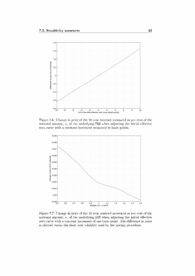
option due to a perturbation of the eective zero rates given by the initial termstructure. Typically the perturbation consists of a constant additive increment3in the range of a few basis points, where a basis point is dened as 10−4. Figure7.6 shows this change in price when varying the increment using the short ratevolatility σ = 0.0075. As is the case when measuring the sensitivity in pricetowards changes in volatility, the gure reveals a linear relation between the∆-value and the size of the increment.The ∆-measure plays a key role for the owner of a Bermudan swaption as it isused for both producing risk estimates as well as constructing hedging positions.Knowing that the value of the short rate volatility very well may alter over timedue to market changes and that the calibration procedure converges quite slowly(and therefore most likely will produce implied volatilities associated with anon-negligible error) it is therefore of interest to study how the ∆-value varieswhen pricing the swaption using dierent short rate volatilities. In gure 7.7the change in price due to a lift corresponding to one basis point is plotted fordierent choices of short rate volatilities. As can be observed in the gure, theabsolute dierence in ∆-value increases slightly as the dierence in short ratevolatility becomes larger.
3Letting y?(0, T ) denote a market observed zero rate with maturity T , the ∆-value cor-responding to an increment α measures the change in price of the Bermudan swaption whenletting y?(0, T )← y?(0, T ) + α for all T ≥ 0.

42 Chapter 7. Numerical results
More specically, the change in the ∆-measure is in the magnitude of 0.001%of the notional amount and is thus quite minor.
7.3. Sensitivity measures 43
−10 −8 −6 −4 −2 0 2 4 6 8 10−0.4
−0.3
−0.2
−0.1
0
0.1
0.2
0.3
0.4
Lift of the initial effective zero curve (basis points)
Diff
eren
ce in
pric
e (%
of n
otio
nal)
Figure 7.6: Change in price of the 10 year contract measured as per cent of thenotional amount, κ, of the underlying IRS when adjusting the initial eectivezero curve with a constant increment measured in basis points.
0.5 0.6 0.7 0.8 0.9 1 1.1 1.2 1.3 1.4 1.50.029
0.03
0.031
0.032
0.033
0.034
0.035
0.036
0.037
0.038
0.039
Multiple of σ = 0.0075
Cha
nge
in p
rice
(% o
f not
iona
l)
Figure 7.7: Change in price of the 10 year contract measured as per cent of thenotional amount, κ, of the underlying IRS when adjusting the initial eectivezero curve with a constant increment of one basis point. The dierence in priceis plotted versus the short rate volatility used by the pricing procedure.

Chapter 8
Summary and conclusions
This thesis has focused on both theoretical and practical aspects of pricingBermudan swaptions. First of all, an exact pricing formula in terms of a Snellenvelope has been derived by solving the optimal stopping problem of pricingthe contract through risk neutral valuation. As this formula has no immediateuse in practical situations due to the fact that it relies on the evaluation of mul-tidimensional integral expressions, a general approximate valuation procedurebased on a recombining binomial tree approximation of the short rate processhas been proposed.Secondly, an explicit pricing formula suited for producing estimate prices ofBermudan swaptions has been proposed by specializing the approximate valu-ation procedure to the Ho-Lee short rate model. Apart from being computa-tionally fast, this procedure also has the benet of being easily calibrated tomarket data as its only required input consists of observed market prices of zerocoupon bonds (an observed discount function) as well as a previous valuationof a Bermudan swaption contract. These properties make the pricing proce-dure particularly useful in situations where estimate prices need to be obtainedquickly using limited market data. In situations such as these, methods used forpricing Bermudan swaptions with high accuracy usually require computation-ally intense procedures when calibrating their parameters to market data. In aworst case scenario some of these methods might not even be able to produceany price at all due to the lack of input needed for calibration.Although some results concerning the behaviour of the specialized pricing methodhave been presented, a topic that remains to be studied is the accuracy of thismethod in terms of calculated price and sensitivity measures compared to moresophisticated pricing procedures using closer approximations of the pricing prob-lem as well as larger sets of observed market data when calibrating. Knowingthe limitations of the Ho-Lee model (cf. the discussion in Chapter 6), it ishowever reasonable to expect that the prices rendered by the suggested pricingprocedure only should be considered as estimates of the true value.
44

Bibliography
[1] Andersen, L. (2000). A Simple Approach to the Pricing of Bermudan Swap-tions in the Multi-Factor Libor Market Model. Journal of Computational
Finance 3, 5-32.[2] Björk, T. (2004). Arbitrage Theory in Continuous Time. Second edition.
Oxford University Press, New York.[3] Brigo, D. & Mercurio, F. (2001). Interest Rate Models: Theory and Prac-
tice. Springer-Verlag, Berlin Heidelberg.[4] Djehiche, B. (2003). Stochastic Calculus: An Introduction with Applica-
tions. Lecture notes. Department of Mathematics. Division of Mathemati-cal Statistics, Royal University of Technology.
[5] Gut, A. (1995). An Intermediate Course in Probability. Springer-Verlag,New York.
[6] Heath, M. T. (2002). Scientic Computing: An Introductory Survey. Sec-ond edition. McGraw-Hill, Boston.
[7] Ho, T. & Lee, S. (1986). Term Structure Movements and Pricing InterestRate Contingent Claims. Journal of Finance 41, 1011-1029.
[8] Hull, J. & White, A. (2001). The General Hull-White Model and Supercal-ibration. Financial Analysts Journal 57, No. 6.
[9] Longsta, F. & Schwartz, E. (2001). Valuing American Options By Simu-lation: A Simple Least Squares Approach. Review of Financial Studies 14,113-148.
[10] Pedersen, M. (1999). Bermudan Swaptions in the LIBOR Market Model.SimCorp Financial Research Working Paper.
[11] Shiryayev, A. N. (1999). Essentials of Stochastic Finance: Facts, Models,
Theory. World Scientic, Singapore.[12] Shiryayev, A. N. (1978). Optimal Stopping Rules. Springer-Verlag, New
York.
45

Appendix A
Pricing zero coupon bonds
using the Ho-Lee binomial
tree
In the following chapter, we provide a derivation of the valuation of zero couponbonds when specifying the dynamics of the short rate process to that suggestedby the Ho-Lee model. Using risk neutral valuation, the value, pm
i,j , at the timeTi and state j of a zero coupon bond having maturity Tm is calculated as
pmi,j = EQ
[e−(ri(Ti+1−Ti)+ri+1(Ti+2−Ti+1)+...+rm−1(Tm−Tm−1)
)∣∣FTi
]= EQ
[e−δ(ri+ri+1+...+rm−1
)∣∣FTi
]
where the relation between the indices i, j and m is given by
i,m = 0, 1, . . . , Ni ≤ mj = −i,−i + 2, . . . , i− 2, i.
Using the denition of the process r given by equation (6.1), we furthermoreget
46

A. Pricing zero coupon bonds using the Ho-Lee binomial tree 47
pmi,j = EQ
[e−δm−1∑k=i
θk e−δ3/2σ( i∑
k=1BQ
k +i+1∑k=1
BQk +...+
m−1∑k=1
BQk
)∣∣FTi
]= e−δ
m−1∑k=i
θk
EQ[e−δ3/2σ
( i∑k=1
BQk +
i+1∑k=1
BQk +...+
m−1∑k=1
BQk
)∣∣FTi
]= e−δ
m−1∑k=i
θk
EQ[e−δ3/2σ(m−i)
i∑k=1
BQk e−δ3/2σ
( i+1∑k=i+1
BQk +...+
m−1∑k=i+1
BQk
)∣∣FTi
].
Since the value process at the time Ti is in state j, it must necessarily hold that
i∑k=1
BQk = j Q-a.s.
and that
i∑k=1
BQk = j
∈ FTi
.
which implies that the exponent storing this sum may be moved outside of theexpectation, i.e.
pmi,j = e−δ
m−1∑k=i
θk−δ3/2σj(m−i)EQ
[e−δ3/2σ( i+1∑
k=i+1BQ
k +...+m−1∑
k=i+1BQ
k
)∣∣FTi
].
We proceed with the calculation by only focusing on the expectation. Restruc-turing the summation results in
EQ[e−δ3/2σ
( i+1∑k=i+1
BQk +...+
m−1∑k=i+1
BQk
)∣∣FTi
]= EQ
[e−δ3/2σm−1∑
k=i+1(m−k)BQ
k ∣∣FTi
]
As the stochastic sequence (Bk)m−1k=i+1 by denition consists of IID symmetric
Bernoulli random variables, the expectation is nally calculated as the product
EQ[e−δ3/2σ
m−1∑k=i+1
(m−k)BQk ∣∣FTi
]=
m−1∏k=i+1
EQ[e−δ3/2σ(m−k)BQ
k
∣∣FTi
]
=m−1∏
k=i+1
cosh(δ3/2σ(m− k)
)

48 A. Pricing zero coupon bonds using the Ho-Lee binomial tree
which in turn determines the value of the process pm at the time Ti and statej as
pmi,j = e−δ
m−1∑k=i
θk−δ3/2σj(m−i)m−1∏
k=i+1
cosh(δ3/2σ(m− k)
)
where the indices i, j and m are given according to the relation
i,m = 0, 1, . . . , Ni ≤ mj = −i,−i + 2, . . . , i− 2, i.


