163
On the Shadow Simplex Method for Curved Polyhedra Daniel Dadush 1 Nicolai H ¨ ahnle 2 1 Centrum Wiskunde & Informatica (CWI) 2 Bonn Universit ¨ at

On the Shadow Simplex Method for CurvedPolyhedra
Daniel Dadush1 Nicolai Hahnle2
1Centrum Wiskunde & Informatica (CWI)
2Bonn Universitat
Outline1 Introduction
Linear Programming and its ApplicationsThe Simplex MethodResults
2 The Shadow Simplex MethodThe Normal FanPrimal and Dual Perspectives
3 Well-conditioned Polytopesτ-wide Polyhedraδ-distance Property
4 Diameter and Optimization3-step Shadow Simplex PathBounding Surface Area Measures of the Normal FanFinding an Optimal Facet
D. Dadush, N. Hahnle Shadow Simplex 2 / 34

Outline1 Introduction
Linear Programming and its ApplicationsThe Simplex MethodResults
2 The Shadow Simplex MethodThe Normal FanPrimal and Dual Perspectives
3 Well-conditioned Polytopesτ-wide Polyhedraδ-distance Property
4 Diameter and Optimization3-step Shadow Simplex PathBounding Surface Area Measures of the Normal FanFinding an Optimal Facet
D. Dadush, N. Hahnle Shadow Simplex 3 / 34

Linear and Integer Programming
Linear Programming (LP): linear constraints & linear objective withcontinuous variables.
max cT xsubject to Ax ≤ b, x ∈ Rn
D. Dadush, N. Hahnle Shadow Simplex 4 / 34

Linear and Integer Programming
Linear Programming (LP): linear constraints & linear objective withcontinuous variables.
max cT xsubject to Ax ≤ b, x ∈ Rn
Amazingly versatile modeling language.Generally provides a “relaxed” view of a desired optimizationproblem, but can be solved in polynomial time via interior point(and many other) methods!
D. Dadush, N. Hahnle Shadow Simplex 4 / 34
Linear and Integer Programming
Linear Programming (LP): linear constraints & linear objective withcontinuous variables.
max cT xsubject to Ax ≤ b, x ∈ Rn
Amazingly versatile modeling language.Generally provides a “relaxed” view of a desired optimizationproblem, but can be solved in polynomial time via interior point(and many other) methods!Will focus on one of the most used classes of algorithms for LP:the Simplex Method (not a polytime algorithm!).
D. Dadush, N. Hahnle Shadow Simplex 4 / 34

Linear and Integer Programming
Mixed Integer Programming (MIP): models both continuous anddiscrete choices.
max cT x + dT ysubject to Ax + Cy ≤ b, x ∈ Rn1 , y ∈ Zn2
D. Dadush, N. Hahnle Shadow Simplex 4 / 34

Linear and Integer Programming
Mixed Integer Programming (MIP): models both continuous anddiscrete choices.
max cT x + dT ysubject to Ax + Cy ≤ b, x ∈ Rn1 , y ∈ Zn2
One of the most successful modeling language for many realworld applications. While instances can be extremely hard tosolve (MIP is NP-hard), many practical instances are not.
D. Dadush, N. Hahnle Shadow Simplex 4 / 34

Linear and Integer Programming
Mixed Integer Programming (MIP): models both continuous anddiscrete choices.
max cT x + dT ysubject to Ax + Cy ≤ b, x ∈ Rn1 , y ∈ Zn2
One of the most successful modeling language for many realworld applications. While instances can be extremely hard tosolve (MIP is NP-hard), many practical instances are not.Many sophisticated software packages exist for these models(CPLEX, Gurobi, etc.). MIP solving is now considered a matureand practical technology.
D. Dadush, N. Hahnle Shadow Simplex 4 / 34

Sample Applications
Routing delivery / pickup trucks for customers.
D. Dadush, N. Hahnle Shadow Simplex 5 / 34

Sample Applications
Optimizing supply chain logistics.
D. Dadush, N. Hahnle Shadow Simplex 5 / 34

Standard Framework for Solving MIPs
Relax integrality of the variables.
D. Dadush, N. Hahnle Shadow Simplex 6 / 34

Standard Framework for Solving MIPs
Relax integrality of the variables.
max cT x + dT ysubject to Ax + Cy ≤ b, x ∈ Rn1 , y ∈ Zn2
D. Dadush, N. Hahnle Shadow Simplex 6 / 34

Standard Framework for Solving MIPs
Relax integrality of the variables.
max cT x + dT ysubject to Ax + Cy ≤ b, x ∈ Rn1 , y ∈ Rn2
D. Dadush, N. Hahnle Shadow Simplex 6 / 34
Standard Framework for Solving MIPs
Relax integrality of the variables.
max cT x + dT ysubject to Ax + Cy ≤ b, x ∈ Rn1 , y ∈ Rn2
Solve the LP.
D. Dadush, N. Hahnle Shadow Simplex 6 / 34

Standard Framework for Solving MIPs
Relax integrality of the variables.
max cT x + dT ysubject to Ax + Cy ≤ b, x ∈ Rn1 , y ∈ Rn2
Solve the LP.Add extra constraints to tighten the LP or “guess” the values ofsome of the integer variables. Repeat.
D. Dadush, N. Hahnle Shadow Simplex 6 / 34

Standard Framework for Solving MIPs
Relax integrality of the variables.
max cT x + dT ysubject to Ax + Cy ≤ b, x ∈ Rn1 , y ∈ Rn2
Solve the LP.Add extra constraints to tighten the LP or “guess” the values ofsome of the integer variables. Repeat.Need to solve a lot of LPs quickly.
D. Dadush, N. Hahnle Shadow Simplex 6 / 34

Linear Programming via the Simplex Method
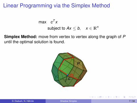
max cT xsubject to Ax ≤ b, x ∈ Rn
Simplex Method: move from vertex to vertex along the graph of Puntil the optimal solution is found.
P
v1c v2
cv3c
v4c v5
c v6c
v7c
v8c
D. Dadush, N. Hahnle Shadow Simplex 7 / 34

Linear Programming via the Simplex Method
max cT xsubject to Ax ≤ b, x ∈ Rn
Simplex Method: move from vertex to vertex along the graph of Puntil the optimal solution is found.
P
v1c
v2cv3
cv4
c v5c v6
cv7
cv8
c
D. Dadush, N. Hahnle Shadow Simplex 7 / 34

Linear Programming via the Simplex Method
max cT xsubject to Ax ≤ b, x ∈ Rn
Simplex Method: move from vertex to vertex along the graph of Puntil the optimal solution is found.
P
v1c
v2c
v3c
v4c v5
c v6c
v7c
v8c
D. Dadush, N. Hahnle Shadow Simplex 7 / 34

Linear Programming via the Simplex Method
max cT xsubject to Ax ≤ b, x ∈ Rn
Simplex Method: move from vertex to vertex along the graph of Puntil the optimal solution is found.
P
v1c v2
c
v3c
v4c v5
c v6c
v7c
v8c
D. Dadush, N. Hahnle Shadow Simplex 7 / 34

Linear Programming via the Simplex Method
max cT xsubject to Ax ≤ b, x ∈ Rn
Simplex Method: move from vertex to vertex along the graph of Puntil the optimal solution is found.
P
v1c v2
cv3c
v4c
v5c v6
cv7
cv8
c
D. Dadush, N. Hahnle Shadow Simplex 7 / 34
Linear Programming via the Simplex Method
max cT xsubject to Ax ≤ b, x ∈ Rn
Simplex Method: move from vertex to vertex along the graph of Puntil the optimal solution is found.
P
v1c v2
cv3c
v4c
v5c
v6c
v7c
v8c
D. Dadush, N. Hahnle Shadow Simplex 7 / 34

Linear Programming via the Simplex Method
max cT xsubject to Ax ≤ b, x ∈ Rn
Simplex Method: move from vertex to vertex along the graph of Puntil the optimal solution is found.
P
v1c v2
cv3c
v4c v5
c
v6c
v7c
v8c
D. Dadush, N. Hahnle Shadow Simplex 7 / 34

Linear Programming via the Simplex Method
max cT xsubject to Ax ≤ b, x ∈ Rn
Simplex Method: move from vertex to vertex along the graph of Puntil the optimal solution is found.
P
v1c v2
cv3c
v4c v5
c v6c
v7c
v8c
D. Dadush, N. Hahnle Shadow Simplex 7 / 34

Linear Programming via the Simplex Method
max cT xsubject to Ax ≤ b, x ∈ Rn
Simplex Method: move from vertex to vertex along the graph of Puntil the optimal solution is found.
P
v1c v2
cv3c
v4c v5
c v6c
v7c
v8c
D. Dadush, N. Hahnle Shadow Simplex 7 / 34
Linear Programming via the Simplex Method
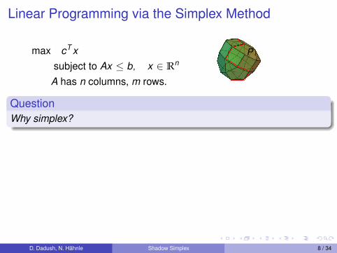
max cT xsubject to Ax ≤ b, x ∈ Rn
A has n columns, m rows.
P
QuestionWhy simplex?
D. Dadush, N. Hahnle Shadow Simplex 8 / 34

Linear Programming via the Simplex Method
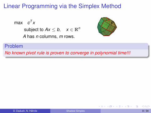
max cT xsubject to Ax ≤ b, x ∈ Rn
A has n columns, m rows.
P
QuestionWhy simplex?
Simplex pivots implementable using “simple” linear algebra.
D. Dadush, N. Hahnle Shadow Simplex 8 / 34

Linear Programming via the Simplex Method
max cT xsubject to Ax ≤ b, x ∈ Rn
A has n columns, m rows.
P
QuestionWhy simplex?
Simplex pivots implementable using “simple” linear algebra.Vertex solutions are often “nice” (e.g. sparse, easy to interpret).
D. Dadush, N. Hahnle Shadow Simplex 8 / 34

Linear Programming via the Simplex Method
max cT xsubject to Ax ≤ b, x ∈ Rn
A has n columns, m rows.
P
QuestionWhy simplex?
Simplex pivots implementable using “simple” linear algebra.Vertex solutions are often “nice” (e.g. sparse, easy to interpret).Terminates with combinatorial description of an optimal solution.
D. Dadush, N. Hahnle Shadow Simplex 8 / 34

Linear Programming via the Simplex Method
max cT xsubject to Ax ≤ b, x ∈ Rn
A has n columns, m rows.
P
QuestionWhy simplex?
Simplex pivots implementable using “simple” linear algebra.Vertex solutions are often “nice” (e.g. sparse, easy to interpret).Terminates with combinatorial description of an optimal solution.“Easy” to reoptimize when adding an extra variable (dual to addinga constraint).
D. Dadush, N. Hahnle Shadow Simplex 8 / 34
Linear Programming via the Simplex Method
max cT xsubject to Ax ≤ b, x ∈ Rn
A has n columns, m rows.
P
ProblemNo known pivot rule is proven to converge in polynomial time!!!
D. Dadush, N. Hahnle Shadow Simplex 8 / 34
Linear Programming via the Simplex Method
max cT xsubject to Ax ≤ b, x ∈ Rn
A has n columns, m rows.
P
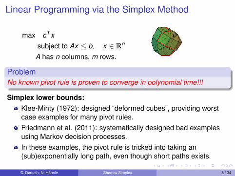
ProblemNo known pivot rule is proven to converge in polynomial time!!!
Simplex lower bounds:Klee-Minty (1972): designed “deformed cubes”, providing worstcase examples for many pivot rules.Friedmann et al. (2011): systematically designed bad examplesusing Markov decision processes.In these examples, the pivot rule is tricked into taking an(sub)exponentially long path, even though short paths exists.
D. Dadush, N. Hahnle Shadow Simplex 8 / 34

Linear Programming via the Simplex Method
max cT xsubject to Ax ≤ b, x ∈ Rn
A has n columns, m rows.
P
ProblemNo known pivot rule is proven to converge in polynomial time!!!
Simplex upper bounds:Kalai (1992): Random facet rule requires 2O(
√n log m) pivots on
expectation.
D. Dadush, N. Hahnle Shadow Simplex 8 / 34

Linear Programming and the Hirsch Conjecture
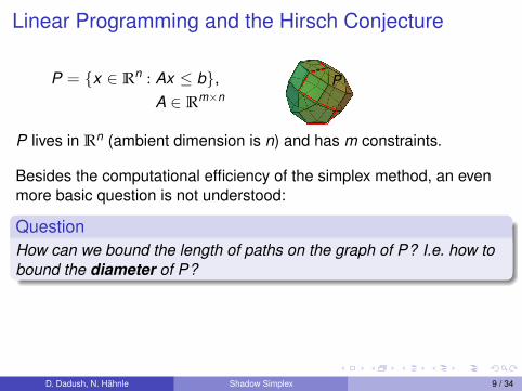
P = {x ∈ Rn : Ax ≤ b},A ∈ Rm×n
P
P lives in Rn (ambient dimension is n) and has m constraints.
D. Dadush, N. Hahnle Shadow Simplex 9 / 34
Linear Programming and the Hirsch Conjecture
P = {x ∈ Rn : Ax ≤ b},A ∈ Rm×n
P
P lives in Rn (ambient dimension is n) and has m constraints.
Besides the computational efficiency of the simplex method, an evenmore basic question is not understood:
QuestionHow can we bound the length of paths on the graph of P? I.e. how tobound the diameter of P?
D. Dadush, N. Hahnle Shadow Simplex 9 / 34

Linear Programming and the Hirsch Conjecture
P = {x ∈ Rn : Ax ≤ b},A ∈ Rm×n
P
P lives in Rn (ambient dimension is n) and has m constraints.
Conjecture (Polynomial Hirsch Conjecture)The diameter of P is bounded by a polynomial in the dimension n andnumber of constraints m.
Diameter lower bounds:Santos (2010), Matschke-Santos-Weibel (2012):Disproved original Hirsch conjecture bound of m− n,exhibit polytopes with diameter (1 + ε)m (for some small ε > 0).
D. Dadush, N. Hahnle Shadow Simplex 9 / 34

Linear Programming and the Hirsch Conjecture
P = {x ∈ Rn : Ax ≤ b},A ∈ Rm×n
P
P lives in Rn (ambient dimension is n) and has m constraints.
Conjecture (Polynomial Hirsch Conjecture)The diameter of P is bounded by a polynomial in the dimension n andnumber of constraints m.
Diameter upper bounds:Barnette, Larman (1974): 1
32n−2(m− n + 52 ).
Kalai, Kleitman (1992), Todd (2014): (m− n)log n.
D. Dadush, N. Hahnle Shadow Simplex 9 / 34

Special Cases
P = {x ∈ Rn : Ax ≤ b}, A ∈ Qm×n
Upper bounds for combinatorial classes:
0/1-polytopes: m− n (Naddef 1989)flow polytopes: quadratic (Orlin 1997)transportation polytopes: linear (Brightwell, v.d. Heuvel andStougie 2006)polars of flag polytopes: m− n (Adripasito, Benedetti 2014)
D. Dadush, N. Hahnle Shadow Simplex 10 / 34

Special Cases
P = {x ∈ Rn : Ax ≤ b}, A ∈ Qm×n
Upper bounds for well-conditioned constraint matrices:
Dyer, Frieze (1994):If A is totally unimodular, diameter is O(m16n3 log(mn)3).
I Analyze a random walk based simplex. They solve LP in similarruntime.
Bonifas, Di Summa, Eisenbrand, Hahnle, Niemeier (2012):If A integer matrix and all subdeterminants ≤ ∆, diameter isO(n3.5∆2 log n∆).
I Use volume expansion on the normal fan (non-constructive!).
D. Dadush, N. Hahnle Shadow Simplex 11 / 34
Simplex Algorithms
P = {x ∈ Rn : Ax ≤ b}, A ∈ Zm×n
Subdeterminants of A bounded by ∆.
QuestionCan the diameter bound of Bonifas et al bounds be madeconstructive? How fast can we solve LP in this setting?
Brunsch, Roglin (2013):Given two vertices can find a path of length O(mn3∆4) efficiently.
I Use shadow simplex method, inspired by smoothed analysis.Eisenbrand, Vempala (2014):Given an initial vertex and objective, can optimize using poly(n,∆)simplex pivots. Initial feasible vertex using m poly(n,∆) pivots.
I Use random walk based dual simplex, similar to Dyer and Frieze.All the above results hold with respect to more general conditionson P (more details later).
D. Dadush, N. Hahnle Shadow Simplex 12 / 34
Simplex Algorithms
P = {x ∈ Rn : Ax ≤ b}, A ∈ Zm×n
Subdeterminants of A bounded by ∆.
QuestionCan the diameter bound of Bonifas et al bounds be madeconstructive? How fast can we solve LP in this setting?
Brunsch, Roglin (2013):Given two vertices can find a path of length O(mn3∆4) efficiently.
I Use shadow simplex method, inspired by smoothed analysis.
Eisenbrand, Vempala (2014):Given an initial vertex and objective, can optimize using poly(n,∆)simplex pivots. Initial feasible vertex using m poly(n,∆) pivots.
I Use random walk based dual simplex, similar to Dyer and Frieze.All the above results hold with respect to more general conditionson P (more details later).
D. Dadush, N. Hahnle Shadow Simplex 12 / 34

Simplex Algorithms
P = {x ∈ Rn : Ax ≤ b}, A ∈ Zm×n
Subdeterminants of A bounded by ∆.
QuestionCan the diameter bound of Bonifas et al bounds be madeconstructive? How fast can we solve LP in this setting?
Brunsch, Roglin (2013):Given two vertices can find a path of length O(mn3∆4) efficiently.
I Use shadow simplex method, inspired by smoothed analysis.Eisenbrand, Vempala (2014):Given an initial vertex and objective, can optimize using poly(n,∆)simplex pivots. Initial feasible vertex using m poly(n,∆) pivots.
I Use random walk based dual simplex, similar to Dyer and Frieze.All the above results hold with respect to more general conditionson P (more details later).
D. Dadush, N. Hahnle Shadow Simplex 12 / 34

Simplex Algorithms
P = {x ∈ Rn : Ax ≤ b}, A ∈ Zm×n
Subdeterminants of A bounded by ∆.
QuestionCan the diameter bound of Bonifas et al bounds be madeconstructive? How fast can we solve LP in this setting?
Brunsch, Roglin (2013):Given two vertices can find a path of length O(mn3∆4) efficiently.
I Use shadow simplex method, inspired by smoothed analysis.Eisenbrand, Vempala (2014):Given an initial vertex and objective, can optimize using poly(n,∆)simplex pivots. Initial feasible vertex using m poly(n,∆) pivots.
I Use random walk based dual simplex, similar to Dyer and Frieze.
All the above results hold with respect to more general conditionson P (more details later).
D. Dadush, N. Hahnle Shadow Simplex 12 / 34

Simplex Algorithms
P = {x ∈ Rn : Ax ≤ b}, A ∈ Zm×n
Subdeterminants of A bounded by ∆.
QuestionCan the diameter bound of Bonifas et al bounds be madeconstructive? How fast can we solve LP in this setting?
Brunsch, Roglin (2013):Given two vertices can find a path of length O(mn3∆4) efficiently.
I Use shadow simplex method, inspired by smoothed analysis.Eisenbrand, Vempala (2014):Given an initial vertex and objective, can optimize using poly(n,∆)simplex pivots. Initial feasible vertex using m poly(n,∆) pivots.
I Use random walk based dual simplex, similar to Dyer and Frieze.All the above results hold with respect to more general conditionson P (more details later).D. Dadush, N. Hahnle Shadow Simplex 12 / 34

A Faster Shadow Simplex Method
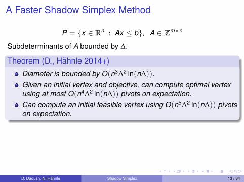
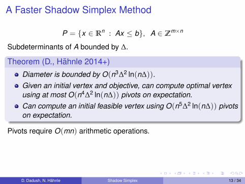
P = {x ∈ Rn : Ax ≤ b}, A ∈ Zm×n
Subdeterminants of A bounded by ∆.
Theorem (D., Hahnle 2014+)
Diameter is bounded by O(n3∆2 ln(n∆)).
Given an initial vertex and objective, can compute optimal vertexusing at most O(n4∆2 ln(n∆)) pivots on expectation.Can compute an initial feasible vertex using O(n5∆2 ln(n∆)) pivotson expectation.
Pivots require O(mn) arithmetic operations.
Based on a new analysis and variant of the shadow simplex method.Inspired by path finding algorithm over the Voronoi graph of a lattice byBonifas, D. (2014) used for solving the Closest Vector Problem.
D. Dadush, N. Hahnle Shadow Simplex 13 / 34

A Faster Shadow Simplex Method
P = {x ∈ Rn : Ax ≤ b}, A ∈ Zm×n
Subdeterminants of A bounded by ∆.
Theorem (D., Hahnle 2014+)
Diameter is bounded by O(n3∆2 ln(n∆)).Given an initial vertex and objective, can compute optimal vertexusing at most O(n4∆2 ln(n∆)) pivots on expectation.
Can compute an initial feasible vertex using O(n5∆2 ln(n∆)) pivotson expectation.
Pivots require O(mn) arithmetic operations.
Based on a new analysis and variant of the shadow simplex method.Inspired by path finding algorithm over the Voronoi graph of a lattice byBonifas, D. (2014) used for solving the Closest Vector Problem.
D. Dadush, N. Hahnle Shadow Simplex 13 / 34
A Faster Shadow Simplex Method
P = {x ∈ Rn : Ax ≤ b}, A ∈ Zm×n
Subdeterminants of A bounded by ∆.
Theorem (D., Hahnle 2014+)
Diameter is bounded by O(n3∆2 ln(n∆)).Given an initial vertex and objective, can compute optimal vertexusing at most O(n4∆2 ln(n∆)) pivots on expectation.Can compute an initial feasible vertex using O(n5∆2 ln(n∆)) pivotson expectation.
Pivots require O(mn) arithmetic operations.
Based on a new analysis and variant of the shadow simplex method.Inspired by path finding algorithm over the Voronoi graph of a lattice byBonifas, D. (2014) used for solving the Closest Vector Problem.
D. Dadush, N. Hahnle Shadow Simplex 13 / 34

A Faster Shadow Simplex Method
P = {x ∈ Rn : Ax ≤ b}, A ∈ Zm×n
Subdeterminants of A bounded by ∆.
Theorem (D., Hahnle 2014+)
Diameter is bounded by O(n3∆2 ln(n∆)).Given an initial vertex and objective, can compute optimal vertexusing at most O(n4∆2 ln(n∆)) pivots on expectation.Can compute an initial feasible vertex using O(n5∆2 ln(n∆)) pivotson expectation.
Pivots require O(mn) arithmetic operations.
Based on a new analysis and variant of the shadow simplex method.
Inspired by path finding algorithm over the Voronoi graph of a lattice byBonifas, D. (2014) used for solving the Closest Vector Problem.
D. Dadush, N. Hahnle Shadow Simplex 13 / 34

A Faster Shadow Simplex Method
P = {x ∈ Rn : Ax ≤ b}, A ∈ Zm×n
Subdeterminants of A bounded by ∆.
Theorem (D., Hahnle 2014+)
Diameter is bounded by O(n3∆2 ln(n∆)).Given an initial vertex and objective, can compute optimal vertexusing at most O(n4∆2 ln(n∆)) pivots on expectation.Can compute an initial feasible vertex using O(n5∆2 ln(n∆)) pivotson expectation.
Pivots require O(mn) arithmetic operations.
Based on a new analysis and variant of the shadow simplex method.Inspired by path finding algorithm over the Voronoi graph of a lattice byBonifas, D. (2014) used for solving the Closest Vector Problem.
D. Dadush, N. Hahnle Shadow Simplex 13 / 34
Navigation over the Voronoi Graph
x
yt
Z + t
Z
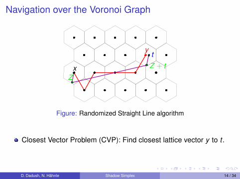
Figure: Randomized Straight Line algorithm
Closest Vector Problem (CVP): Find closest lattice vector y to t .
D. Dadush, N. Hahnle Shadow Simplex 14 / 34

Navigation over the Voronoi Graph
x
yt
Z + t
Z
Figure: Randomized Straight Line algorithm
Closest Vector Problem (CVP): Find closest lattice vector y to t .Solving CVP can be reduced to efficiently navigating over theVoronoi cell (Som.,Fed.,Shal. 09; Mic.,Voulg. 10-13).
D. Dadush, N. Hahnle Shadow Simplex 14 / 34
Navigation over the Voronoi Graph
x
yt
Z + t
Z
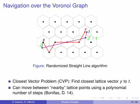
Figure: Randomized Straight Line algorithm
Closest Vector Problem (CVP): Find closest lattice vector y to t .Can move between “nearby” lattice points using a polynomialnumber of steps (Bonifas, D. 14).
D. Dadush, N. Hahnle Shadow Simplex 14 / 34

Outline1 Introduction
Linear Programming and its ApplicationsThe Simplex MethodResults
2 The Shadow Simplex MethodThe Normal FanPrimal and Dual Perspectives
3 Well-conditioned Polytopesτ-wide Polyhedraδ-distance Property
4 Diameter and Optimization3-step Shadow Simplex PathBounding Surface Area Measures of the Normal FanFinding an Optimal Facet
D. Dadush, N. Hahnle Shadow Simplex 15 / 34

The Polar
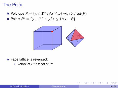
Polytope P = {x ∈ Rn : Ax ≤ b} with 0 ∈ int(P)
Polar: P? = {y ∈ Rn : yT x ≤ 1 ∀x ∈ P}
Face lattice is reversed:I vertex of P ∼= facet of P?
I k -face of P ∼= (n− k − 1)-face of P?
I vertex-edge path in P ∼= facet-ridge path in P?
D. Dadush, N. Hahnle Shadow Simplex 16 / 34
The Polar
Polytope P = {x ∈ Rn : Ax ≤ b} with 0 ∈ int(P)
Polar: P? = {y ∈ Rn : yT x ≤ 1 ∀x ∈ P}
Face lattice is reversed:I vertex of P ∼= facet of P?
I k -face of P ∼= (n− k − 1)-face of P?
I vertex-edge path in P ∼= facet-ridge path in P?
D. Dadush, N. Hahnle Shadow Simplex 16 / 34

The Polar
Polytope P = {x ∈ Rn : Ax ≤ b} with 0 ∈ int(P)
Polar: P? = {y ∈ Rn : yT x ≤ 1 ∀x ∈ P}
Face lattice is reversed:I vertex of P ∼= facet of P?
I k -face of P ∼= (n− k − 1)-face of P?
I vertex-edge path in P ∼= facet-ridge path in P?
D. Dadush, N. Hahnle Shadow Simplex 16 / 34

The Polar
Polytope P = {x ∈ Rn : Ax ≤ b} with 0 ∈ int(P)
Polar: P? = {y ∈ Rn : yT x ≤ 1 ∀x ∈ P}
Face lattice is reversed:I vertex of P ∼= facet of P?
I k -face of P ∼= (n− k − 1)-face of P?
I vertex-edge path in P ∼= facet-ridge path in P?
D. Dadush, N. Hahnle Shadow Simplex 16 / 34

The Polar
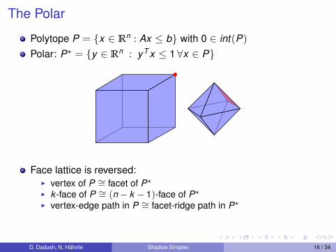
Polytope P = {x ∈ Rn : Ax ≤ b} with 0 ∈ int(P)
Polar: P? = {y ∈ Rn : yT x ≤ 1 ∀x ∈ P}
Face lattice is reversed:I vertex of P ∼= facet of P?
I k -face of P ∼= (n− k − 1)-face of P?
I vertex-edge path in P ∼= facet-ridge path in P?
D. Dadush, N. Hahnle Shadow Simplex 16 / 34

The Polar
Polytope P = {x ∈ Rn : Ax ≤ b} with 0 ∈ int(P)
Polar: P? = {y ∈ Rn : yT x ≤ 1 ∀x ∈ P}
Face lattice is reversed:I vertex of P ∼= facet of P?
I k -face of P ∼= (n− k − 1)-face of P?
I vertex-edge path in P ∼= facet-ridge path in P?
D. Dadush, N. Hahnle Shadow Simplex 16 / 34

The Polar
Polytope P = {x ∈ Rn : Ax ≤ b} with 0 ∈ int(P)
Polar: P? = {y ∈ Rn : yT x ≤ 1 ∀x ∈ P}
Face lattice is reversed:I vertex of P ∼= facet of P?
I k -face of P ∼= (n− k − 1)-face of P?
I vertex-edge path in P ∼= facet-ridge path in P?
D. Dadush, N. Hahnle Shadow Simplex 16 / 34
The Polar
Polytope P = {x ∈ Rn : Ax ≤ b} with 0 ∈ int(P)
Polar: P? = {y ∈ Rn : yT x ≤ 1 ∀x ∈ P}
Face lattice is reversed:I vertex of P ∼= facet of P?
I k -face of P ∼= (n− k − 1)-face of P?
I vertex-edge path in P ∼= facet-ridge path in P?
D. Dadush, N. Hahnle Shadow Simplex 16 / 34

The Normal Fan
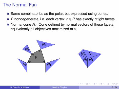
Same combinatorics as the polar, but expressed using cones.
P nondegenerate, i.e. each vertex v ∈ P has exactly n tight facets.Normal cone Nv : Cone defined by normal vectors of these facets,equivalently all objectives maximized at v .Normal fan: Set of all normal cones.
N3
N1
N4N2
PN3 N1
N4N2
v1
v2
v3
v4
D. Dadush, N. Hahnle Shadow Simplex 17 / 34

The Normal Fan
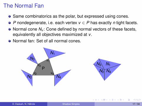
Same combinatorics as the polar, but expressed using cones.P nondegenerate, i.e. each vertex v ∈ P has exactly n tight facets.
Normal cone Nv : Cone defined by normal vectors of these facets,equivalently all objectives maximized at v .Normal fan: Set of all normal cones.
N3
N1
N4N2
PN3 N1
N4N2
v1
v2
v3
v4
D. Dadush, N. Hahnle Shadow Simplex 17 / 34
The Normal Fan
Same combinatorics as the polar, but expressed using cones.P nondegenerate, i.e. each vertex v ∈ P has exactly n tight facets.Normal cone Nv : Cone defined by normal vectors of these facets,equivalently all objectives maximized at v .
Normal fan: Set of all normal cones.
N3
N1
N4N2
PN3 N1
N4N2
v1
v2
v3
v4
D. Dadush, N. Hahnle Shadow Simplex 17 / 34
The Normal Fan
Same combinatorics as the polar, but expressed using cones.P nondegenerate, i.e. each vertex v ∈ P has exactly n tight facets.Normal cone Nv : Cone defined by normal vectors of these facets,equivalently all objectives maximized at v .Normal fan: Set of all normal cones.
N3
N1
N4N2
PN3 N1
N4N2
v1
v2
v3
v4
D. Dadush, N. Hahnle Shadow Simplex 17 / 34

The Shadow Simplex Method
v ′2
dv ′1
c
v2 v1
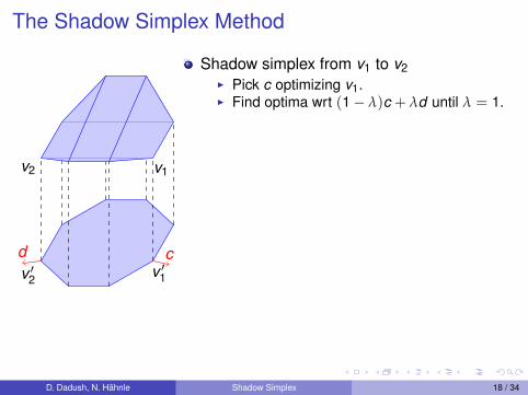
Shadow simplex from v1 to v2I Pick c optimizing v1.I Find optima wrt (1− λ)c + λd until λ = 1.
“Primal” interpretationI Project P to span of c and d .I Optima wrt (1− λ)c + λd are pre-images of
optima in the plane.“Dual” interpretation
I Trace segment [c,d ] through normal fan.I Pivot step corresponds to crossing facet of a
normal cone.
D. Dadush, N. Hahnle Shadow Simplex 18 / 34
The Shadow Simplex Method
v ′2
dv ′1
c
v2 v1
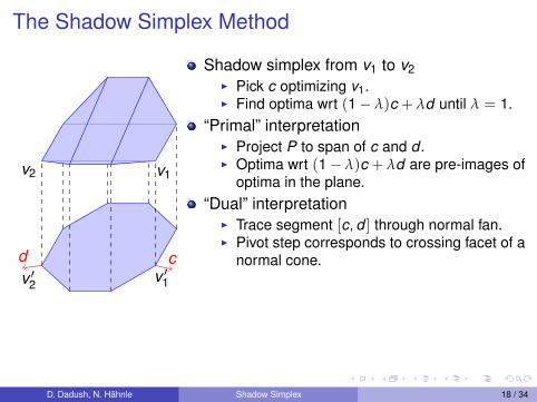
Shadow simplex from v1 to v2I Pick c optimizing v1.I Find optima wrt (1− λ)c + λd until λ = 1.
“Primal” interpretationI Project P to span of c and d .I Optima wrt (1− λ)c + λd are pre-images of
optima in the plane.“Dual” interpretation
I Trace segment [c,d ] through normal fan.I Pivot step corresponds to crossing facet of a
normal cone.
D. Dadush, N. Hahnle Shadow Simplex 18 / 34

The Shadow Simplex Method
v ′2
dv ′1
c
v2 v1
Shadow simplex from v1 to v2I Pick c optimizing v1.I Find optima wrt (1− λ)c + λd until λ = 1.
“Primal” interpretationI Project P to span of c and d .I Optima wrt (1− λ)c + λd are pre-images of
optima in the plane.
“Dual” interpretationI Trace segment [c,d ] through normal fan.I Pivot step corresponds to crossing facet of a
normal cone.
D. Dadush, N. Hahnle Shadow Simplex 18 / 34
The Shadow Simplex Method
v ′2
dv ′1
c
v2 v1
Shadow simplex from v1 to v2I Pick c optimizing v1.I Find optima wrt (1− λ)c + λd until λ = 1.
“Primal” interpretationI Project P to span of c and d .I Optima wrt (1− λ)c + λd are pre-images of
optima in the plane.“Dual” interpretation
I Trace segment [c,d ] through normal fan.I Pivot step corresponds to crossing facet of a
normal cone.
D. Dadush, N. Hahnle Shadow Simplex 18 / 34

Size of the shadow: randomness to the rescue
QuestionWhen can we bound the number of edges in the shadow?
In general, the shadow can be exponentially large.
Borgwardt (1980s), Spielman-Teng (2004), Vershynin (2006): theshadow is small in expectation when the linear program is randomor smoothed.Brunsch-Roglin (2013): the shadow is small in expectation for“well-conditioned” polytopes when c,d are randomly chosen fromthe normal cones of two vertices.
D. Dadush, N. Hahnle Shadow Simplex 19 / 34

Size of the shadow: randomness to the rescue
QuestionWhen can we bound the number of edges in the shadow?
In general, the shadow can be exponentially large.Borgwardt (1980s), Spielman-Teng (2004), Vershynin (2006): theshadow is small in expectation when the linear program is randomor smoothed.
Brunsch-Roglin (2013): the shadow is small in expectation for“well-conditioned” polytopes when c,d are randomly chosen fromthe normal cones of two vertices.
D. Dadush, N. Hahnle Shadow Simplex 19 / 34

Size of the shadow: randomness to the rescue
QuestionWhen can we bound the number of edges in the shadow?
In general, the shadow can be exponentially large.Borgwardt (1980s), Spielman-Teng (2004), Vershynin (2006): theshadow is small in expectation when the linear program is randomor smoothed.Brunsch-Roglin (2013): the shadow is small in expectation for“well-conditioned” polytopes when c,d are randomly chosen fromthe normal cones of two vertices.
D. Dadush, N. Hahnle Shadow Simplex 19 / 34

Shadow Simplex: Dual Perspective
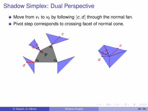
Move from v1 to v2 by following [c,d ] through the normal fan.Pivot step corresponds to crossing facet of normal cone.
P
v1
v2
v3
v4
c
d
c
d
D. Dadush, N. Hahnle Shadow Simplex 20 / 34

Shadow Simplex: Dual Perspective
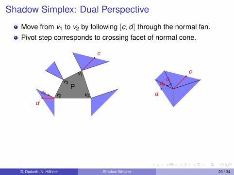
Move from v1 to v2 by following [c,d ] through the normal fan.Pivot step corresponds to crossing facet of normal cone.
P
v1
v2
v3
v4
c
d
c
d
D. Dadush, N. Hahnle Shadow Simplex 20 / 34

Shadow Simplex: Dual Perspective
Move from v1 to v2 by following [c,d ] through the normal fan.Pivot step corresponds to crossing facet of normal cone.
P
v1
v2
v3
v4
c
d
c
d
d1
d1
D. Dadush, N. Hahnle Shadow Simplex 20 / 34

Shadow Simplex: Dual Perspective
Move from v1 to v2 by following [c,d ] through the normal fan.Pivot step corresponds to crossing facet of normal cone.
P
v1
v2
v3
v4
c
d
c
d
d1
d1
D. Dadush, N. Hahnle Shadow Simplex 20 / 34
Shadow Simplex: Dual Perspective
Move from v1 to v2 by following [c,d ] through the normal fan.Pivot step corresponds to crossing facet of normal cone.
P
v1
v2
v3
v4
c
d
c
d
d1d2
d1d2
D. Dadush, N. Hahnle Shadow Simplex 20 / 34
Shadow Simplex: Dual Perspective
Move from v1 to v2 by following [c,d ] through the normal fan.Pivot step corresponds to crossing facet of normal cone.
P
v1
v2
v3
v4
c
d
c
d
d1d2
d2
D. Dadush, N. Hahnle Shadow Simplex 20 / 34

Shadow Simplex: Dual Perspective
Move from v1 to v2 by following [c,d ] through the normal fan.Pivot step corresponds to crossing facet of normal cone.
P
v1
v2
v3
v4
c
d
c
dd2
d2
D. Dadush, N. Hahnle Shadow Simplex 20 / 34

Shadow Simplex: Dual Perspective
Move from v1 to v2 by following [c,d ] through the normal fan.Pivot step corresponds to crossing facet of normal cone.
P
v1
v2
v3
v4
c
d
c
d
QuestionHow can we bound the number of intersections with the normal fan?
D. Dadush, N. Hahnle Shadow Simplex 20 / 34

Outline1 Introduction
Linear Programming and its ApplicationsThe Simplex MethodResults
2 The Shadow Simplex MethodThe Normal FanPrimal and Dual Perspectives
3 Well-conditioned Polytopesτ-wide Polyhedraδ-distance Property
4 Diameter and Optimization3-step Shadow Simplex PathBounding Surface Area Measures of the Normal FanFinding an Optimal Facet
D. Dadush, N. Hahnle Shadow Simplex 21 / 34

Polyhedra with τ-wide Normal Fan
Vertex normal cone Nv is τ-wide:contains a ball of radius τ centeredon the unit sphere.
N3
N1
N4N2
P
v1
v2
v3
v4
a1
a2
a3
Nv
Nvτ
D. Dadush, N. Hahnle Shadow Simplex 22 / 34

Polyhedra with τ-wide Normal Fan
Vertex normal cone Nv is τ-wide:contains a ball of radius τ centeredon the unit sphere.
N3
N1
N4N2
P
v1
v2
v3
v4
a1
a2
a3
Nv
Nvτ
D. Dadush, N. Hahnle Shadow Simplex 22 / 34

Polyhedra with τ-wide Normal Fan
Vertex normal cone Nv is τ-wide:contains a ball of radius τ centeredon the unit sphere.P is τ-wide if all its vertex normalcones are τ-wide.
N3
N1
N4N2
P
v1
v2
v3
v4
a1
a2
a3
Nv
Nvτ
D. Dadush, N. Hahnle Shadow Simplex 22 / 34

Polyhedra with τ-wide Normal Fan
Vertex normal cone Nv is τ-wide:contains a ball of radius τ centeredon the unit sphere.Angles at any vertex are less thanπ − 2τ. “Discrete measure” ofcurvature.
N3
N1
N4N2
P
v1
v2
v3
v4
a1
a2
a3
Nv
Nvτ
D. Dadush, N. Hahnle Shadow Simplex 22 / 34

Polyhedra with τ-wide Normal Fan
a1
a2
a3
Nvτ
D. Dadush, N. Hahnle Shadow Simplex 23 / 34
Polyhedra with τ-wide Normal Fan
a1
a2
a3
Nvτ
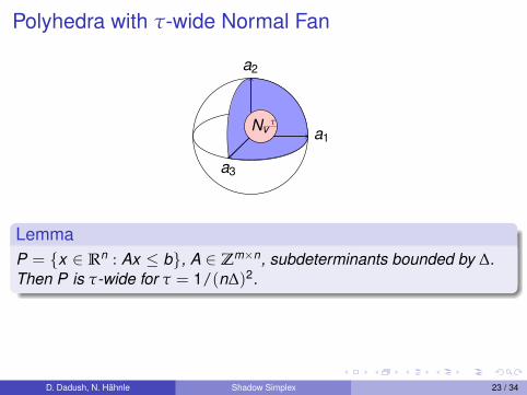
LemmaP = {x ∈ Rn : Ax ≤ b}, A ∈ Zm×n, subdeterminants bounded by ∆.Then P is τ-wide for τ = 1/(n∆)2.
D. Dadush, N. Hahnle Shadow Simplex 23 / 34

Polyhedra with τ-wide Normal Fan
a1
a2
a3
Nvτ
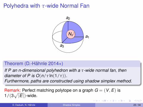
Theorem (D.-Hahnle 2014+)If P an n-dimensional polyhedron with a τ-wide normal fan, thendiameter of P is O(n/τ ln(1/τ)).
Furthermore, paths are constructed using shadow simplex method.
Remark: Perfect matching polytope on a graph G = (V ,E) is1/(3
√|E |)-wide.
D. Dadush, N. Hahnle Shadow Simplex 23 / 34

Polyhedra with τ-wide Normal Fan
a1
a2
a3
Nvτ
Theorem (D.-Hahnle 2014+)If P an n-dimensional polyhedron with a τ-wide normal fan, thendiameter of P is O(n/τ ln(1/τ)).Furthermore, paths are constructed using shadow simplex method.
Remark: Perfect matching polytope on a graph G = (V ,E) is1/(3
√|E |)-wide.
D. Dadush, N. Hahnle Shadow Simplex 23 / 34
The δ-distance Property
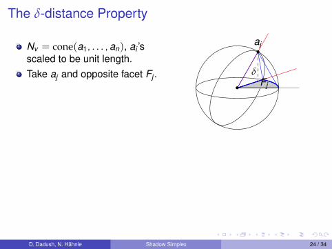
Nv = cone(a1, . . . ,an), ai ’sscaled to be unit length.Take aj and opposite facet Fj .
δ-distance property:d(aj ,H(Fj)) ≥ δ for allfacet/opposite vertex pairs
aj
Fj
δ
D. Dadush, N. Hahnle Shadow Simplex 24 / 34
The δ-distance Property
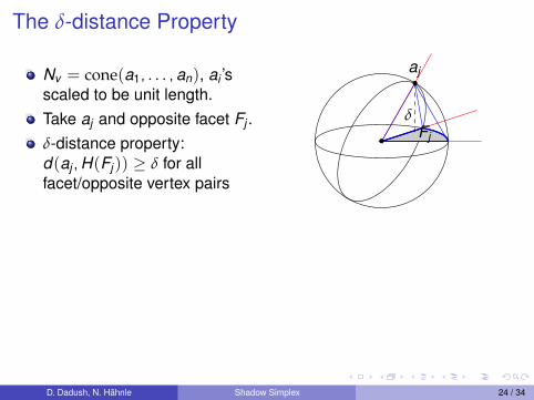
Nv = cone(a1, . . . ,an), ai ’sscaled to be unit length.Take aj and opposite facet Fj .δ-distance property:d(aj ,H(Fj)) ≥ δ for allfacet/opposite vertex pairs
aj
Fj
δ
D. Dadush, N. Hahnle Shadow Simplex 24 / 34

The δ-distance Property
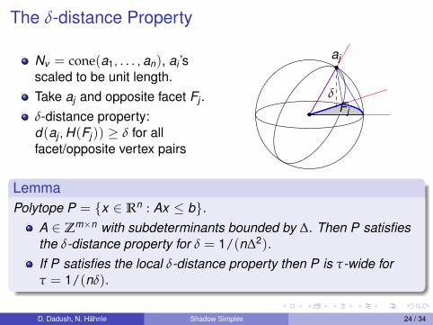
Nv = cone(a1, . . . ,an), ai ’sscaled to be unit length.Take aj and opposite facet Fj .δ-distance property:d(aj ,H(Fj)) ≥ δ for allfacet/opposite vertex pairs
aj
Fj
δ
P has the (local) δ-distance property ifevery (feasible) basis has the δ-distance property.
D. Dadush, N. Hahnle Shadow Simplex 24 / 34

The δ-distance Property
Nv = cone(a1, . . . ,an), ai ’sscaled to be unit length.Take aj and opposite facet Fj .δ-distance property:d(aj ,H(Fj)) ≥ δ for allfacet/opposite vertex pairs
aj
Fj
δ
LemmaPolytope P = {x ∈ Rn : Ax ≤ b}.
A ∈ Zm×n with subdeterminants bounded by ∆. Then P satisfiesthe δ-distance property for δ = 1/(n∆2).
If P satisfies the local δ-distance property then P is τ-wide forτ = 1/(nδ).
D. Dadush, N. Hahnle Shadow Simplex 24 / 34
The δ-distance Property
Nv = cone(a1, . . . ,an), ai ’sscaled to be unit length.Take aj and opposite facet Fj .δ-distance property:d(aj ,H(Fj)) ≥ δ for allfacet/opposite vertex pairs
aj
Fj
δ
LemmaPolytope P = {x ∈ Rn : Ax ≤ b}.
A ∈ Zm×n with subdeterminants bounded by ∆. Then P satisfiesthe δ-distance property for δ = 1/(n∆2).If P satisfies the local δ-distance property then P is τ-wide forτ = 1/(nδ).
D. Dadush, N. Hahnle Shadow Simplex 24 / 34

The δ-distance Property
Nv = cone(a1, . . . ,an), ai ’sscaled to be unit length.Take aj and opposite facet Fj .δ-distance property:d(aj ,H(Fj)) ≥ δ for allfacet/opposite vertex pairs
aj
Fj
δ
Theorem (D.-Hahnle)If P a polytope satisfying local δ-distance property, then given afeasible vertex and objective, an optimal vertex can be found usingO(n3/δ ln(n/δ)) shadow simplex pivots.
Resolves question of Vempala and Eisenbrand (2014) regardingsufficiency of local δ-distance property for optimization.
D. Dadush, N. Hahnle Shadow Simplex 24 / 34

Outline1 Introduction
Linear Programming and its ApplicationsThe Simplex MethodResults
2 The Shadow Simplex MethodThe Normal FanPrimal and Dual Perspectives
3 Well-conditioned Polytopesτ-wide Polyhedraδ-distance Property
4 Diameter and Optimization3-step Shadow Simplex PathBounding Surface Area Measures of the Normal FanFinding an Optimal Facet
D. Dadush, N. Hahnle Shadow Simplex 25 / 34

3-step Shadow Simplex PathTo bound the diameter, we will exhibit a short shadow simplex pathbetween any two vertices.
Let v ,w be vertices of P.
Pick c ∈ Nv , d ∈ Nw to be “deep” inside the respective normalcones (exact choice made later).Let X be exponentially distributed over Rn, that is with probabilitydensity proportional to e−‖x‖.We shall follow the simplex paths in sequence:
c(a)−→ c + X
(b)−→ d + X(c)−→ d
QuestionHow long is this path?
D. Dadush, N. Hahnle Shadow Simplex 26 / 34
3-step Shadow Simplex PathTo bound the diameter, we will exhibit a short shadow simplex pathbetween any two vertices.
Let v ,w be vertices of P.Pick c ∈ Nv , d ∈ Nw to be “deep” inside the respective normalcones (exact choice made later).
Let X be exponentially distributed over Rn, that is with probabilitydensity proportional to e−‖x‖.We shall follow the simplex paths in sequence:
c(a)−→ c + X
(b)−→ d + X(c)−→ d
QuestionHow long is this path?
D. Dadush, N. Hahnle Shadow Simplex 26 / 34

3-step Shadow Simplex PathTo bound the diameter, we will exhibit a short shadow simplex pathbetween any two vertices.
Let v ,w be vertices of P.Pick c ∈ Nv , d ∈ Nw to be “deep” inside the respective normalcones (exact choice made later).Let X be exponentially distributed over Rn, that is with probabilitydensity proportional to e−‖x‖.
We shall follow the simplex paths in sequence:
c(a)−→ c + X
(b)−→ d + X(c)−→ d
QuestionHow long is this path?
D. Dadush, N. Hahnle Shadow Simplex 26 / 34

3-step Shadow Simplex PathTo bound the diameter, we will exhibit a short shadow simplex pathbetween any two vertices.
Let v ,w be vertices of P.Pick c ∈ Nv , d ∈ Nw to be “deep” inside the respective normalcones (exact choice made later).Let X be exponentially distributed over Rn, that is with probabilitydensity proportional to e−‖x‖.We shall follow the simplex paths in sequence:
c(a)−→ c + X
(b)−→ d + X(c)−→ d
QuestionHow long is this path?
D. Dadush, N. Hahnle Shadow Simplex 26 / 34

Crossing Bounds
The 3-step shadow simplex path:
c(a)−→ c + X
(b)−→ d + X(c)−→ d
Theorem (D.-Hahnle)Assume P is an n-dimensional τ-wide polyhedron.
Phase (b). The expected number of crossings of [c + X ,d + X ]with normal fan of P is bounded by O(‖c − d‖/τ).Phase (a+c). The expected number of crossings of[c + αX , c + X ] and [d + αX ,d + X ], for α ∈ (0,1],with normal fan of P is O(n/τ ln(1/α)).
Remark: Only bound intersections of partial path in phases (a) and (c).Next up: Diameter and Phase (b) crossing bound.
D. Dadush, N. Hahnle Shadow Simplex 27 / 34

Crossing Bounds
The 3-step shadow simplex path:
c(a)−→ c + X
(b)−→ d + X(c)−→ d
Theorem (D.-Hahnle)Assume P is an n-dimensional τ-wide polyhedron.
Phase (b). The expected number of crossings of [c + X ,d + X ]with normal fan of P is bounded by O(‖c − d‖/τ).
Phase (a+c). The expected number of crossings of[c + αX , c + X ] and [d + αX ,d + X ], for α ∈ (0,1],with normal fan of P is O(n/τ ln(1/α)).
Remark: Only bound intersections of partial path in phases (a) and (c).Next up: Diameter and Phase (b) crossing bound.
D. Dadush, N. Hahnle Shadow Simplex 27 / 34

Crossing Bounds
The 3-step shadow simplex path:
c(a)−→ c + X
(b)−→ d + X(c)−→ d
Theorem (D.-Hahnle)Assume P is an n-dimensional τ-wide polyhedron.
Phase (b). The expected number of crossings of [c + X ,d + X ]with normal fan of P is bounded by O(‖c − d‖/τ).Phase (a+c). The expected number of crossings of[c + αX , c + X ] and [d + αX ,d + X ], for α ∈ (0,1],with normal fan of P is O(n/τ ln(1/α)).
Remark: Only bound intersections of partial path in phases (a) and (c).Next up: Diameter and Phase (b) crossing bound.
D. Dadush, N. Hahnle Shadow Simplex 27 / 34

Crossing Bounds
The 3-step shadow simplex path:
c(a)−→ c + X
(b)−→ d + X(c)−→ d
Theorem (D.-Hahnle)Assume P is an n-dimensional τ-wide polyhedron.
Phase (b). The expected number of crossings of [c + X ,d + X ]with normal fan of P is bounded by O(‖c − d‖/τ).Phase (a+c). The expected number of crossings of[c + αX , c + X ] and [d + αX ,d + X ], for α ∈ (0,1],with normal fan of P is O(n/τ ln(1/α)).
Remark: Only bound intersections of partial path in phases (a) and (c).
Next up: Diameter and Phase (b) crossing bound.
D. Dadush, N. Hahnle Shadow Simplex 27 / 34

Crossing Bounds
The 3-step shadow simplex path:
c(a)−→ c + X
(b)−→ d + X(c)−→ d
Theorem (D.-Hahnle)Assume P is an n-dimensional τ-wide polyhedron.
Phase (b). The expected number of crossings of [c + X ,d + X ]with normal fan of P is bounded by O(‖c − d‖/τ).Phase (a+c). The expected number of crossings of[c + αX , c + X ] and [d + αX ,d + X ], for α ∈ (0,1],with normal fan of P is O(n/τ ln(1/α)).
Remark: Only bound intersections of partial path in phases (a) and (c).Next up: Diameter and Phase (b) crossing bound.
D. Dadush, N. Hahnle Shadow Simplex 27 / 34
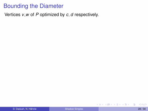
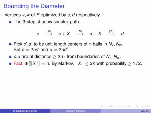
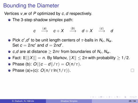
Bounding the DiameterVertices v ,w of P optimized by c,d respectively.
The 3-step shadow simplex path:
c(a)−→ c + X
(b)−→ d + X(c)−→ d
Pick c′,d ′ to be unit length centers of τ-balls in Nv ,Nw .Set c = 2nc′ and d = 2nd ′.c,d are at distance ≥ 2nτ from boundaries of Nv ,Nw .Fact: E[‖X‖] = n. By Markov, ‖X‖ ≤ 2n with probability ≥ 1/2.
D. Dadush, N. Hahnle Shadow Simplex 28 / 34

Bounding the DiameterVertices v ,w of P optimized by c,d respectively.
The 3-step shadow simplex path:
c(a)−→ c + X
(b)−→ d + X(c)−→ d
How to choose c and d?
Pick c′,d ′ to be unit length centers of τ-balls in Nv ,Nw .Set c = 2nc′ and d = 2nd ′.c,d are at distance ≥ 2nτ from boundaries of Nv ,Nw .Fact: E[‖X‖] = n. By Markov, ‖X‖ ≤ 2n with probability ≥ 1/2.
D. Dadush, N. Hahnle Shadow Simplex 28 / 34

Bounding the DiameterVertices v ,w of P optimized by c,d respectively.
The 3-step shadow simplex path:
c(a)−→ c + X
(b)−→ d + X(c)−→ d
Pick c′,d ′ to be unit length centers of τ-balls in Nv ,Nw .Set c = 2nc′ and d = 2nd ′.
c,d are at distance ≥ 2nτ from boundaries of Nv ,Nw .Fact: E[‖X‖] = n. By Markov, ‖X‖ ≤ 2n with probability ≥ 1/2.
D. Dadush, N. Hahnle Shadow Simplex 28 / 34

Bounding the DiameterVertices v ,w of P optimized by c,d respectively.
The 3-step shadow simplex path:
c(a)−→ c + X
(b)−→ d + X(c)−→ d
Pick c′,d ′ to be unit length centers of τ-balls in Nv ,Nw .Set c = 2nc′ and d = 2nd ′.c,d are at distance ≥ 2nτ from boundaries of Nv ,Nw .
Fact: E[‖X‖] = n. By Markov, ‖X‖ ≤ 2n with probability ≥ 1/2.
D. Dadush, N. Hahnle Shadow Simplex 28 / 34
Bounding the DiameterVertices v ,w of P optimized by c,d respectively.
The 3-step shadow simplex path:
c(a)−→ c + X
(b)−→ d + X(c)−→ d
Pick c′,d ′ to be unit length centers of τ-balls in Nv ,Nw .Set c = 2nc′ and d = 2nd ′.c,d are at distance ≥ 2nτ from boundaries of Nv ,Nw .Fact: E[‖X‖] = n. By Markov, ‖X‖ ≤ 2n with probability ≥ 1/2.
D. Dadush, N. Hahnle Shadow Simplex 28 / 34

Bounding the DiameterVertices v ,w of P optimized by c,d respectively.
The 3-step shadow simplex path:
c(a)−→ c + X
(b)−→ d + X(c)−→ d
Pick c′,d ′ to be unit length centers of τ-balls in Nv ,Nw .Set c = 2nc′ and d = 2nd ′.c,d are at distance ≥ 2nτ from boundaries of Nv ,Nw .Fact: E[‖X‖] = n. By Markov, ‖X‖ ≤ 2n with probability ≥ 1/2.If ‖X‖ ≤ 2n, c + τX ,d + τX are in Nv ,Nw .
D. Dadush, N. Hahnle Shadow Simplex 28 / 34

Bounding the DiameterVertices v ,w of P optimized by c,d respectively.
The 3-step shadow simplex path:
c(a)−→ c + X
(b)−→ d + X(c)−→ d
Pick c′,d ′ to be unit length centers of τ-balls in Nv ,Nw .Set c = 2nc′ and d = 2nd ′.c,d are at distance ≥ 2nτ from boundaries of Nv ,Nw .Fact: E[‖X‖] = n. By Markov, ‖X‖ ≤ 2n with probability ≥ 1/2.If ‖X‖ ≤ 2n, c + τX ,d + τX are in Nv ,Nw .Need only bound crossings for [c + τX , c + X ], [d + τX ,d + X ]!
D. Dadush, N. Hahnle Shadow Simplex 28 / 34
Bounding the DiameterVertices v ,w of P optimized by c,d respectively.
The 3-step shadow simplex path:
c(a)−→ c + X
(b)−→ d + X(c)−→ d
Pick c′,d ′ to be unit length centers of τ-balls in Nv ,Nw .Set c = 2nc′ and d = 2nd ′.c,d are at distance ≥ 2nτ from boundaries of Nv ,Nw .Fact: E[‖X‖] = n. By Markov, ‖X‖ ≤ 2n with probability ≥ 1/2.Phase (b): O(‖c − d‖/τ) = O(n/τ).Phase (a)+(c): O(n/τ ln(1/τ)).
D. Dadush, N. Hahnle Shadow Simplex 28 / 34

Bounding the DiameterVertices v ,w of P optimized by c,d respectively.
The 3-step shadow simplex path:
c(a)−→ c + X
(b)−→ d + X(c)−→ d
Pick c′,d ′ to be unit length centers of τ-balls in Nv ,Nw .Set c = 2nc′ and d = 2nd ′.c,d are at distance ≥ 2nτ from boundaries of Nv ,Nw .Fact: E[‖X‖] = n. By Markov, ‖X‖ ≤ 2n with probability ≥ 1/2.Phase (b): O(‖c − d‖/τ) = O(n/τ).Phase (a)+(c): O(n/τ ln(1/τ)).Remark: Can bound diameter using only phase (b) by scaling c,dup by 1/τ, so that c/τ + X ,d/τ + X stay in Nv ,Nw respectively.
D. Dadush, N. Hahnle Shadow Simplex 28 / 34

Bounding the DiameterVertices v ,w of P optimized by c,d respectively.
The 3-step shadow simplex path:
c(a)−→ c + X
(b)−→ d + X(c)−→ d
Pick c′,d ′ to be unit length centers of τ-balls in Nv ,Nw .Set c = 2nc′ and d = 2nd ′.c,d are at distance ≥ 2nτ from boundaries of Nv ,Nw .Fact: E[‖X‖] = n. By Markov, ‖X‖ ≤ 2n with probability ≥ 1/2.Phase (b): O(‖c − d‖/τ) = O(n/τ).Phase (a)+(c): O(n/τ ln(1/τ)).Remark: Can bound diameter using only phase (b) by scaling c,dup by 1/τ, so that c/τ + X ,d/τ + X stay in Nv ,Nw respectively.Results in O(n/δ2) diameter bound.
D. Dadush, N. Hahnle Shadow Simplex 28 / 34

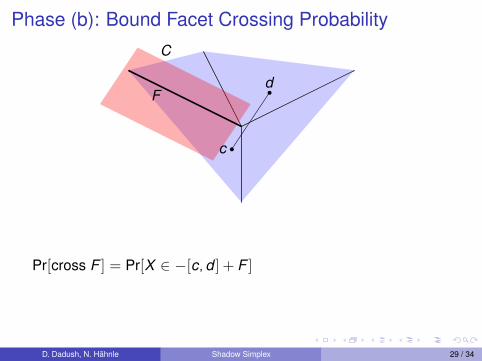
Phase (b): Bound Facet Crossing Probability
F
C
c
d
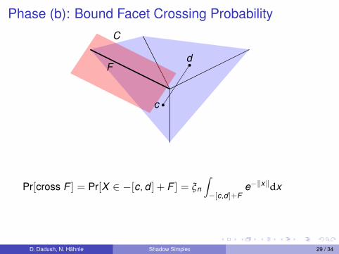
Pr[cross F ] = Pr[X ∈ −[c,d ] + F ]
= ξn
∫−[c,d ]+F
e−‖x‖dx
= ξnuT (d − c)∫ 1
0
∫F−((1−λ)c+λd)
e−‖x‖d voln−1(x)dλ
D. Dadush, N. Hahnle Shadow Simplex 29 / 34

Phase (b): Bound Facet Crossing Probability
F
C
c + X
d + X
Pr[cross F ] = Pr[X ∈ −[c,d ] + F ]
= ξn
∫−[c,d ]+F
e−‖x‖dx
= ξnuT (d − c)∫ 1
0
∫F−((1−λ)c+λd)
e−‖x‖d voln−1(x)dλ
D. Dadush, N. Hahnle Shadow Simplex 29 / 34
Phase (b): Bound Facet Crossing Probability
F
C
c
d
Pr[cross F ] = Pr[X ∈ −[c,d ] + F ]
= ξn
∫−[c,d ]+F
e−‖x‖dx
= ξnuT (d − c)∫ 1
0
∫F−((1−λ)c+λd)
e−‖x‖d voln−1(x)dλ
D. Dadush, N. Hahnle Shadow Simplex 29 / 34
Phase (b): Bound Facet Crossing Probability
F
C
c
d
Pr[cross F ] = Pr[X ∈ −[c,d ] + F ] = ξn
∫−[c,d ]+F
e−‖x‖dx
= ξnuT (d − c)∫ 1
0
∫F−((1−λ)c+λd)
e−‖x‖d voln−1(x)dλ
D. Dadush, N. Hahnle Shadow Simplex 29 / 34
Phase (b): Bound Facet Crossing Probability
F
C
c
du
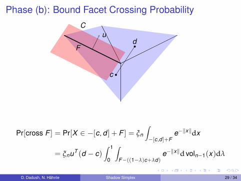
Pr[cross F ] = Pr[X ∈ −[c,d ] + F ] = ξn
∫−[c,d ]+F
e−‖x‖dx
= ξnuT (d − c)∫ 1
0
∫F−((1−λ)c+λd)
e−‖x‖d voln−1(x)dλ
D. Dadush, N. Hahnle Shadow Simplex 29 / 34
Bounding the Surface Measure using τ
F
Nv
u
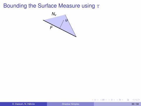
The set {F + t + R+y : F facet of Nv} forms a partition of Nv + t .∫F+t+R+y
e−‖x‖dx =∫ ∞
0
∫F+t+ r
h ye−‖x‖d voln−1(x)dr
=∫ ∞
0
∫F+t
e−‖x+rh y‖d voln−1(x)dr
≥∫ ∞
0e−r/hdr
∫F+t
e−‖x‖d voln−1(x)
≥ τ∫
F+te−‖x‖d voln−1(x)
D. Dadush, N. Hahnle Shadow Simplex 30 / 34

Bounding the Surface Measure using τ
F
Nv
u
t
yh
τ
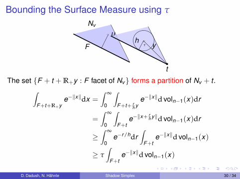
The set {F + t + R+y : F facet of Nv} forms a partition of Nv + t .
∫F+t+R+y
e−‖x‖dx =∫ ∞
0
∫F+t+ r
h ye−‖x‖d voln−1(x)dr
=∫ ∞
0
∫F+t
e−‖x+rh y‖d voln−1(x)dr
≥∫ ∞
0e−r/hdr
∫F+t
e−‖x‖d voln−1(x)
≥ τ∫
F+te−‖x‖d voln−1(x)
D. Dadush, N. Hahnle Shadow Simplex 30 / 34

Bounding the Surface Measure using τ
F
Nv
u
t
yh
τ
The set {F + t + R+y : F facet of Nv} forms a partition of Nv + t .∫F+t+R+y
e−‖x‖dx =∫ ∞
0
∫F+t+ r
h ye−‖x‖d voln−1(x)dr
=∫ ∞
0
∫F+t
e−‖x+rh y‖d voln−1(x)dr
≥∫ ∞
0e−r/hdr
∫F+t
e−‖x‖d voln−1(x)
≥ τ∫
F+te−‖x‖d voln−1(x)
D. Dadush, N. Hahnle Shadow Simplex 30 / 34

Bounding the Surface Measure using τ
F
Nv
u
t
yh
τ
The set {F + t + R+y : F facet of Nv} forms a partition of Nv + t .∫F+t+R+y
e−‖x‖dx =∫ ∞
0
∫F+t+ r
h ye−‖x‖d voln−1(x)dr
=∫ ∞
0
∫F+t
e−‖x+rh y‖d voln−1(x)dr
≥∫ ∞
0e−r/hdr
∫F+t
e−‖x‖d voln−1(x)
≥ τ∫
F+te−‖x‖d voln−1(x)
D. Dadush, N. Hahnle Shadow Simplex 30 / 34

Putting it all together
yF
Nv
c
du
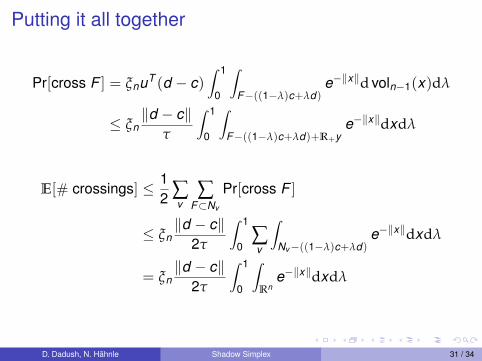
Pr[cross F ] = ξnuT (d − c)∫ 1
0
∫F−((1−λ)c+λd)
e−‖x‖d voln−1(x)dλ
≤ ξn‖d − c‖
τ
∫ 1
0
∫F−((1−λ)c+λd)+R+y
e−‖x‖dxdλ
E[# crossings] ≤ 12 ∑
v∑
F⊂Nv
Pr[cross F ]
≤ ξn‖d − c‖
2τ
∫ 1
0∑v
∫Nv−((1−λ)c+λd)
e−‖x‖dxdλ
= ξn‖d − c‖
2τ
∫ 1
0
∫Rn
e−‖x‖dxdλ
=‖d − c‖
2τ
D. Dadush, N. Hahnle Shadow Simplex 31 / 34

Putting it all together
yF
Nv
c
du
Pr[cross F ] = ξnuT (d − c)∫ 1
0
∫F−((1−λ)c+λd)
e−‖x‖d voln−1(x)dλ
≤ ξn‖d − c‖
τ
∫ 1
0
∫F−((1−λ)c+λd)+R+y
e−‖x‖dxdλ
E[# crossings] ≤ 12 ∑
v∑
F⊂Nv
Pr[cross F ]
≤ ξn‖d − c‖
2τ
∫ 1
0∑v
∫Nv−((1−λ)c+λd)
e−‖x‖dxdλ
= ξn‖d − c‖
2τ
∫ 1
0
∫Rn
e−‖x‖dxdλ
=‖d − c‖
2τ
D. Dadush, N. Hahnle Shadow Simplex 31 / 34

Putting it all together
Pr[cross F ] = ξnuT (d − c)∫ 1
0
∫F−((1−λ)c+λd)
e−‖x‖d voln−1(x)dλ
≤ ξn‖d − c‖
τ
∫ 1
0
∫F−((1−λ)c+λd)+R+y
e−‖x‖dxdλ
E[# crossings] ≤ 12 ∑
v∑
F⊂Nv
Pr[cross F ]
≤ ξn‖d − c‖
2τ
∫ 1
0∑v
∫Nv−((1−λ)c+λd)
e−‖x‖dxdλ
= ξn‖d − c‖
2τ
∫ 1
0
∫Rn
e−‖x‖dxdλ
=‖d − c‖
2τ
D. Dadush, N. Hahnle Shadow Simplex 31 / 34
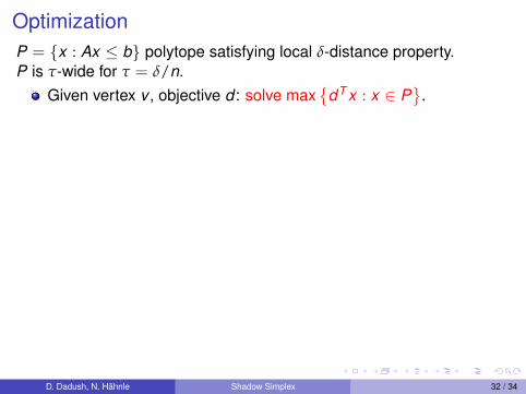
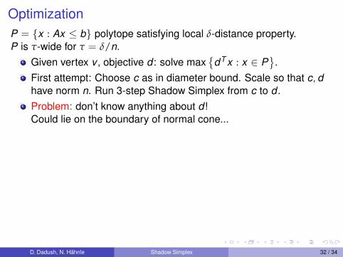
OptimizationP = {x : Ax ≤ b} polytope satisfying local δ-distance property.P is τ-wide for τ = δ/n.
Given vertex v , objective d : solve max{
dT x : x ∈ P}
.
First attempt: Choose c as in diameter bound. Scale so that c,dhave norm n. Run 3-step Shadow Simplex from c to d .Problem: don’t know anything about d !Could lie on the boundary of normal cone...Phase (c) bound: can find vertex w ′ optimizing d ′,‖d ′ − d‖ ≤ nε = ‖d‖ε with O(n/τ ln(1/ε)) pivots.
D. Dadush, N. Hahnle Shadow Simplex 32 / 34

OptimizationP = {x : Ax ≤ b} polytope satisfying local δ-distance property.P is τ-wide for τ = δ/n.
Given vertex v , objective d : solve max{
dT x : x ∈ P}
.First attempt: Choose c as in diameter bound. Scale so that c,dhave norm n. Run 3-step Shadow Simplex from c to d .
Problem: don’t know anything about d !Could lie on the boundary of normal cone...Phase (c) bound: can find vertex w ′ optimizing d ′,‖d ′ − d‖ ≤ nε = ‖d‖ε with O(n/τ ln(1/ε)) pivots.
D. Dadush, N. Hahnle Shadow Simplex 32 / 34
OptimizationP = {x : Ax ≤ b} polytope satisfying local δ-distance property.P is τ-wide for τ = δ/n.
Given vertex v , objective d : solve max{
dT x : x ∈ P}
.First attempt: Choose c as in diameter bound. Scale so that c,dhave norm n. Run 3-step Shadow Simplex from c to d .Problem: don’t know anything about d !Could lie on the boundary of normal cone...
Phase (c) bound: can find vertex w ′ optimizing d ′,‖d ′ − d‖ ≤ nε = ‖d‖ε with O(n/τ ln(1/ε)) pivots.
D. Dadush, N. Hahnle Shadow Simplex 32 / 34

OptimizationP = {x : Ax ≤ b} polytope satisfying local δ-distance property.P is τ-wide for τ = δ/n.
Given vertex v , objective d : solve max{
dT x : x ∈ P}
.First attempt: Choose c as in diameter bound. Scale so that c,dhave norm n. Run 3-step Shadow Simplex from c to d .Problem: don’t know anything about d !Could lie on the boundary of normal cone...Phase (c) bound: can find vertex w ′ optimizing d ′,‖d ′ − d‖ ≤ nε = ‖d‖ε with O(n/τ ln(1/ε)) pivots.
D. Dadush, N. Hahnle Shadow Simplex 32 / 34

OptimizationP = {x : Ax ≤ b} polytope satisfying local δ-distance property.P is τ-wide for τ = δ/n.
Given vertex v , objective d : solve max{
dT x : x ∈ P}
.First attempt: Choose c as in diameter bound. Scale so that c,dhave norm n. Run 3-step Shadow Simplex from c to d .Problem: don’t know anything about d !Could lie on the boundary of normal cone...Phase (c) bound: can find vertex w ′ optimizing d ′,‖d ′ − d‖ ≤ nε = ‖d‖ε with O(n/τ ln(1/ε)) pivots.Remark: already enough for weakly polynomial bound.
D. Dadush, N. Hahnle Shadow Simplex 32 / 34

OptimizationP = {x : Ax ≤ b} polytope satisfying local δ-distance property.P is τ-wide for τ = δ/n.
Given vertex v , objective d : solve max{
dT x : x ∈ P}
.First attempt: Choose c as in diameter bound. Scale so that c,dhave norm n. Run 3-step Shadow Simplex from c to d .Problem: don’t know anything about d !Could lie on the boundary of normal cone...Phase (c) bound: can find vertex w ′ optimizing d ′,‖d ′ − d‖ ≤ nε = ‖d‖ε with O(n/τ ln(1/ε)) pivots.Solution: can identity optimal facet from w and d ′!
D. Dadush, N. Hahnle Shadow Simplex 32 / 34
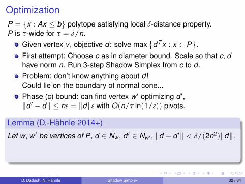
OptimizationP = {x : Ax ≤ b} polytope satisfying local δ-distance property.P is τ-wide for τ = δ/n.
Given vertex v , objective d : solve max{
dT x : x ∈ P}
.First attempt: Choose c as in diameter bound. Scale so that c,dhave norm n. Run 3-step Shadow Simplex from c to d .Problem: don’t know anything about d !Could lie on the boundary of normal cone...Phase (c) bound: can find vertex w ′ optimizing d ′,‖d ′ − d‖ ≤ nε = ‖d‖ε with O(n/τ ln(1/ε)) pivots.
Lemma (D.-Hahnle 2014+)
Let w ,w ′ be vertices of P, d ∈ Nw , d ′ ∈ Nw ′ , ‖d − d ′‖ < δ/(2n2)‖d‖.
Let d ′ = ∑i∈I λiai /‖ai‖, where Nw = cone({ai : i ∈ I}).Then for j = argmaxj∈Iλj , w lies on the facet aT
j x ≤ bj .
D. Dadush, N. Hahnle Shadow Simplex 32 / 34

OptimizationP = {x : Ax ≤ b} polytope satisfying local δ-distance property.P is τ-wide for τ = δ/n.
Given vertex v , objective d : solve max{
dT x : x ∈ P}
.First attempt: Choose c as in diameter bound. Scale so that c,dhave norm n. Run 3-step Shadow Simplex from c to d .Problem: don’t know anything about d !Could lie on the boundary of normal cone...Phase (c) bound: can find vertex w ′ optimizing d ′,‖d ′ − d‖ ≤ nε = ‖d‖ε with O(n/τ ln(1/ε)) pivots.
Lemma (D.-Hahnle 2014+)
Let w ,w ′ be vertices of P, d ∈ Nw , d ′ ∈ Nw ′ , ‖d − d ′‖ < δ/(2n2)‖d‖.Let d ′ = ∑i∈I λiai /‖ai‖, where Nw = cone({ai : i ∈ I}).
Then for j = argmaxj∈Iλj , w lies on the facet aTj x ≤ bj .
D. Dadush, N. Hahnle Shadow Simplex 32 / 34

OptimizationP = {x : Ax ≤ b} polytope satisfying local δ-distance property.P is τ-wide for τ = δ/n.
Given vertex v , objective d : solve max{
dT x : x ∈ P}
.First attempt: Choose c as in diameter bound. Scale so that c,dhave norm n. Run 3-step Shadow Simplex from c to d .Problem: don’t know anything about d !Could lie on the boundary of normal cone...Phase (c) bound: can find vertex w ′ optimizing d ′,‖d ′ − d‖ ≤ nε = ‖d‖ε with O(n/τ ln(1/ε)) pivots.
Lemma (D.-Hahnle 2014+)
Let w ,w ′ be vertices of P, d ∈ Nw , d ′ ∈ Nw ′ , ‖d − d ′‖ < δ/(2n2)‖d‖.Let d ′ = ∑i∈I λiai /‖ai‖, where Nw = cone({ai : i ∈ I}).Then for j = argmaxj∈Iλj , w lies on the facet aT
j x ≤ bj .
D. Dadush, N. Hahnle Shadow Simplex 32 / 34
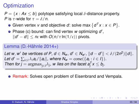
OptimizationP = {x : Ax ≤ b} polytope satisfying local δ-distance property.P is τ-wide for τ = δ/n.
Given vertex v and objective d : solve max{
dT x : x ∈ P}
.Phase (c) bound: can find vertex w optimizing d ′,‖d ′ − d‖ ≤ nε with O(n/τ ln(1/ε)) pivots.
Lemma (D.-Hahnle 2014+)
Let w ,w ′ be vertices of P, d ∈ Nw , d ′ ∈ Nw ′ , ‖d − d ′‖ < δ/(2n2)‖d‖.Let d ′ = ∑i∈I λiai /‖ai‖, where Nw = cone({ai : i ∈ I}).Then for j = argmaxj∈Iλj , w lies on the facet aT
j x ≤ bj .
Remark: Solves open problem of Eisenbrand and Vempala.
D. Dadush, N. Hahnle Shadow Simplex 33 / 34

OptimizationP = {x : Ax ≤ b} polytope satisfying local δ-distance property.P is τ-wide for τ = δ/n.
Given vertex v and objective d : solve max{
dT x : x ∈ P}
.Phase (c) bound: can find vertex w optimizing d ′,‖d ′ − d‖ ≤ nε with O(n/τ ln(1/ε)) pivots.
Lemma (D.-Hahnle 2014+)
Let w ,w ′ be vertices of P, d ∈ Nw , d ′ ∈ Nw ′ , ‖d − d ′‖ < δ/(2n2)‖d‖.Let d ′ = ∑i∈I λiai /‖ai‖, where Nw = cone({ai : i ∈ I}).Then for j = argmaxj∈Iλj , w lies on the facet aT
j x ≤ bj .
Setting ε = δ/(2n2), find an optimal facet afterO(n/τ ln(n/δ)) = O(n2/δ ln(n/δ)) pivots.
D. Dadush, N. Hahnle Shadow Simplex 33 / 34
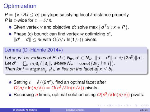
OptimizationP = {x : Ax ≤ b} polytope satisfying local δ-distance property.P is τ-wide for τ = δ/n.
Given vertex v and objective d : solve max{
dT x : x ∈ P}
.Phase (c) bound: can find vertex w optimizing d ′,‖d ′ − d‖ ≤ nε with O(n/τ ln(1/ε)) pivots.
Lemma (D.-Hahnle 2014+)
Let w ,w ′ be vertices of P, d ∈ Nw , d ′ ∈ Nw ′ , ‖d − d ′‖ < δ/(2n2)‖d‖.Let d ′ = ∑i∈I λiai /‖ai‖, where Nw = cone({ai : i ∈ I}).Then for j = argmaxj∈Iλj , w lies on the facet aT
j x ≤ bj .
Setting ε = δ/(2n2), find an optimal facet afterO(n/τ ln(n/δ)) = O(n2/δ ln(n/δ)) pivots.Recursing n times, optimal solution using O(n3/δ ln(n/δ)) pivots.
D. Dadush, N. Hahnle Shadow Simplex 33 / 34

OptimizationP = {x : Ax ≤ b} polytope satisfying local δ-distance property.P is τ-wide for τ = δ/n.
Given vertex v and objective d : solve max{
dT x : x ∈ P}
.Phase (c) bound: can find vertex w optimizing d ′,‖d ′ − d‖ ≤ nε with O(n/τ ln(1/ε)) pivots.
Lemma (D.-Hahnle 2014+)
Let w ,w ′ be vertices of P, d ∈ Nw , d ′ ∈ Nw ′ , ‖d − d ′‖ < δ/(2n2)‖d‖.Let d ′ = ∑i∈I λiai /‖ai‖, where Nw = cone({ai : i ∈ I}).Then for j = argmaxj∈Iλj , w lies on the facet aT
j x ≤ bj .
Feasibility: Use standard reductions to optimization (Phase 1simplex).
D. Dadush, N. Hahnle Shadow Simplex 33 / 34

Summary and Open Problems
New and simpler analysis and variant of the Shadow Simplexmethod.Improved diameter bounds and simplex algorithm for curvedpolyhedra.Inspired by path finding algorithm over the Voronoi graph of alattice by Bonifas, D. (2014) used for solving the Closest VectorProblem.
Open Problems:Improve smoothed analysis bounds using our techniques.Polynomial Hirsch conjecture for random polytopes?When can we improve the geometry of the normal fan?
Thank you!
D. Dadush, N. Hahnle Shadow Simplex 34 / 34

Summary and Open Problems
New and simpler analysis and variant of the Shadow Simplexmethod.Improved diameter bounds and simplex algorithm for curvedpolyhedra.Inspired by path finding algorithm over the Voronoi graph of alattice by Bonifas, D. (2014) used for solving the Closest VectorProblem.
Open Problems:Improve smoothed analysis bounds using our techniques.
Polynomial Hirsch conjecture for random polytopes?When can we improve the geometry of the normal fan?
Thank you!
D. Dadush, N. Hahnle Shadow Simplex 34 / 34

Summary and Open Problems
New and simpler analysis and variant of the Shadow Simplexmethod.Improved diameter bounds and simplex algorithm for curvedpolyhedra.Inspired by path finding algorithm over the Voronoi graph of alattice by Bonifas, D. (2014) used for solving the Closest VectorProblem.
Open Problems:Improve smoothed analysis bounds using our techniques.Polynomial Hirsch conjecture for random polytopes?
When can we improve the geometry of the normal fan?
Thank you!
D. Dadush, N. Hahnle Shadow Simplex 34 / 34

Summary and Open Problems
New and simpler analysis and variant of the Shadow Simplexmethod.Improved diameter bounds and simplex algorithm for curvedpolyhedra.Inspired by path finding algorithm over the Voronoi graph of alattice by Bonifas, D. (2014) used for solving the Closest VectorProblem.
Open Problems:Improve smoothed analysis bounds using our techniques.Polynomial Hirsch conjecture for random polytopes?When can we improve the geometry of the normal fan?
Thank you!
D. Dadush, N. Hahnle Shadow Simplex 34 / 34

Summary and Open Problems
New and simpler analysis and variant of the Shadow Simplexmethod.Improved diameter bounds and simplex algorithm for curvedpolyhedra.Inspired by path finding algorithm over the Voronoi graph of alattice by Bonifas, D. (2014) used for solving the Closest VectorProblem.
Open Problems:Improve smoothed analysis bounds using our techniques.Polynomial Hirsch conjecture for random polytopes?When can we improve the geometry of the normal fan?
Thank you!D. Dadush, N. Hahnle Shadow Simplex 34 / 34


