91
On validation of a wheel-rail wear prediction code
MSc thesis
by
ADRIÁN SÁNCHEZ ARANDOJO
Department of Aeronautical and Vehicle Engineering, Division of Rail Vehicles
TRITA AVE 2013:41ISSN 1651-7660
ISRN KTH/AVE/RTM/-13/41ISBN 978-91-7501-826-3
Postal address: Visiting address: Telephone:Royal Institute of Technology Teknikringen 8 +46 70 6522441Aeronautical and Vehicle Engineering StockholmRail Vehicles E-mail:SE-100 44 Stockholm [email protected]


Preface
This MSc thesis corresponds to the last part of my studies on Mechanical Engineering.It has been carried out at the Division of Rail Vehicles, Department of Aeronautical andVehicle Engineering at the Royal Institute of Technology (KTH) in Stockholm.
I studied the �rst four years of my degree at the Technical University of Madrid (UPM),in the Technical School of Industrial Engineering the specialization of Mechanics of Ma-chines. I was very lucky to have the chance to perform the last year of my degree and myend of studies project at the Royal Institue of Technology in Stockholm.
First of all I would like to thank my supervisor, Carlos Casanueva, for giving me theopportunity of performing the MSc Thesis at the division and for his continuous help andguidance during this work.
I would also like to thank the rest of the people in the division, especially: SaeedHossein Nia, Raphael Schär, Matin Shahzamanian Sichani and Mats Berg.
Thanks to Ingemar Persson from DEsolver, for his patience and his help with GENSYS.
Finally, I would like to thank my friends, Marta and especially my parents for theirconstant support.
June 2013
Adrián Sánchez Arandojo

Abstract
During the past years, several tools have been developed to try predicting wheel and railwear of railway vehicles in an e�cient way. In this MSc thesis a new wear predictiontool developed by I.Persson is studied and compared with another wear prediction tool,developed by T.Jendel, which has been already validated and is in use since several yearsago. The advantages that the new model gives are simpler structure, the consideration ofwear as a continuous variable and that all the code is integrated in the same software.
The two models have the same methodology until the part of the wear calculationsand the post-processing. Wheel-rail geometry functions and time domain simulations areperformed with the software GENSYS.
In the simulation model the track and the vehicle are de�ned as well as other importantproperties such as vehicle speed and coe�cient of friction. Three simple tracks are used:tangent track, R=500 m curve with a cant of ht=0.15 m on the outer rail and R=1000 mcurve with a cant of ht=0.1 m on the outer rail. The model is assumed to be symmetric sojust outer (�rst and fourth axle) and inner (second and third axles) wheels are considered.
During the vehicle-track interaction, the normal and tangential problems are solved.The wheel-rail contact is modelled according to Hertz's theory and Kalker's simpli�edtheory with the help of the algorithm FASTSIM. Then wear calculations are performedaccording to Archard's wear law. It is applied in di�erent ways, obtaining wear depthdirectly in Jendel's and wear volume rate in Persson's model.
Jendel's model is �rstly analyzed. Its speci�c methodology is brie�y explained andmodi�cations are performed on the code to make it work as similar as possible to Persson'smodel. Also parameters regarding the distance in which wear calculations are taken, thediscretization of the width of the wheel and the discretization of the contact patch areanalyzed.
The methodology of Persson's model is also studied, most of all the performance of thepost-processing which is one of the keys to the code. The parameters analyzed in this codeare the ones regarding a statistical analysis performed during the post-processing and thediscretization of the contact patch.
Finally the comparisons between the wear depth obtained for both models are carriedout. The discrepancies between the models are explained with the parameters analyzedand the dynamic behaviour of both models. Also a theoretical case is used as reference forcomparison.
Contents
1 Introduction 1
1.1 Brief background . . . . . . . . . . . . . . . . . . . . . . . . . . . . . . . . . 1
1.2 Evolution of wear prediction tools . . . . . . . . . . . . . . . . . . . . . . . . 2
1.3 Objective of the thesis . . . . . . . . . . . . . . . . . . . . . . . . . . . . . . 4
2 General methodology 7
3 Simulation model 9
3.1 Vehicle characteristics . . . . . . . . . . . . . . . . . . . . . . . . . . . . . . 9
3.2 Track geometry . . . . . . . . . . . . . . . . . . . . . . . . . . . . . . . . . . 10
3.3 Other important characteristics of the model . . . . . . . . . . . . . . . . . 10
3.4 Symmetric track . . . . . . . . . . . . . . . . . . . . . . . . . . . . . . . . . 11
4 Vehicle-track interaction 13
4.1 Coordinate system . . . . . . . . . . . . . . . . . . . . . . . . . . . . . . . . 13
4.2 Wheel-rail geometry functions . . . . . . . . . . . . . . . . . . . . . . . . . . 14
4.3 Normal contact problem . . . . . . . . . . . . . . . . . . . . . . . . . . . . . 15
4.4 Tangential contact problem . . . . . . . . . . . . . . . . . . . . . . . . . . . 16
5 Wear calculations 21
5.1 Wear calculations of Jendel's model . . . . . . . . . . . . . . . . . . . . . . . 22
5.2 Wear calculations of Persson's model . . . . . . . . . . . . . . . . . . . . . . 23
5.3 Example of wheel wear . . . . . . . . . . . . . . . . . . . . . . . . . . . . . . 23
6 Reference code: T.Jendel's model 25
6.1 Methodology . . . . . . . . . . . . . . . . . . . . . . . . . . . . . . . . . . . 25
6.1.1 Modi�cations of Jendel's code . . . . . . . . . . . . . . . . . . . . . . 27
6.2 Results and discussion . . . . . . . . . . . . . . . . . . . . . . . . . . . . . . 28
6.2.1 Discretization of the width of the wheel, dy . . . . . . . . . . . . . . 28
6.2.2 Sampling of the wear calculations, L_sample . . . . . . . . . . . . . 30
6.2.3 Discretization of the contact ellipse, m and n . . . . . . . . . . . . . 31

7 Code to validate: I.Persson's model 33
7.1 Methodology . . . . . . . . . . . . . . . . . . . . . . . . . . . . . . . . . . . 33
7.1.1 Post-processing . . . . . . . . . . . . . . . . . . . . . . . . . . . . . . 34
7.2 Results and discussion . . . . . . . . . . . . . . . . . . . . . . . . . . . . . . 38
7.2.1 Number of intervals of the Xname axis, Nintx . . . . . . . . . . . . 38
7.2.2 Number of intervals of the Iname axis, Ninty . . . . . . . . . . . . . 40
7.2.3 Discretization of the contact patch, m and n parameters . . . . . . . 42
8 Comparisons 45
8.1 Comparison of the dynamic behaviour . . . . . . . . . . . . . . . . . . . . . 45
8.2 Comparison of the wear depth between the two models after running 280 m 48
8.2.1 R=500 m curve case . . . . . . . . . . . . . . . . . . . . . . . . . . . 49
8.2.2 R=1000 m curve case . . . . . . . . . . . . . . . . . . . . . . . . . . 51
8.3 Comparison of the wear depth between the two models after running 5.6 km 55
8.4 Comparison with the theoretical case . . . . . . . . . . . . . . . . . . . . . 56
8.4.1 Methodology . . . . . . . . . . . . . . . . . . . . . . . . . . . . . . . 56
8.4.2 Results and discussion . . . . . . . . . . . . . . . . . . . . . . . . . . 56
9 Conclusions and future work 59
Bibliography 61
Appendices
A Notations 63
B Comparisons wheel by wheel 67
B.1 R=500 m curve case . . . . . . . . . . . . . . . . . . . . . . . . . . . . . . . 67
B.2 R=1000 m curve case . . . . . . . . . . . . . . . . . . . . . . . . . . . . . . 71
C Results of the analysis of the parameters 77
C.1 Jendel's model . . . . . . . . . . . . . . . . . . . . . . . . . . . . . . . . . . 77
C.2 Persson's model . . . . . . . . . . . . . . . . . . . . . . . . . . . . . . . . . . 80

Chapter 1
Introduction
When railway vehicles run on tracks, contact forces are transferred between wheels and railsthrough the contact patches. These tangential and normal contact forces allow the vehicleto run over the track. Nevertheless when sliding occurs, it can lead to material removalor plastic deformation both of rails and wheels producing a change in the geometry of thepro�les. This change in the geometry of the pro�les is a really important issue since it canchange the dynamic behaviour of the vehicle.
One of these causes of change in the geometry, material removal, can nowadays bepredicted through wear prediction tools. These wear prediction tools are codes developedto know the evolution of the wear, thus the evolution of the pro�les, without having to runthousands of kilometers and take pro�le measurements at every speci�c distance.
1.1 Brief background
The previously mentioned material removal will be referred to as wear in the followingsections. Wear a�ects both wheels and rails. Wheel wear (Figure 1.1) can be separated inseveral types [1]:
� Wheel �ange wear: Flange thickness tf is reduced. This is normally produced dueto higher creepages and creep forces because of higher coe�cient of friction; smallercurve radius and horizontally sti�er wheelset suspension along with longer wheelsetbase.
� Wheel tread wear: Both �ange height hf and thickness tf are increased, normallybecause of combinations of normal forces with large or ordinary creep forces.
� Wheel out-of-roundness: There are several types such as eccentricity of the wheelsdue to non-centred position of the wheel when pro�ling; wheel �ats when duringbraking the wheels are locked and thus do not rotate, and waves or corrugationsbecause of waves around the perimeter due to vibrations in the wheel-rail system.
1

CHAPTER 1. INTRODUCTION
Figure 1.1: Quantities for wheel wear (mm) [1]
On the other hand rail wear can also be classi�ed in several types:
� Rail gauge corner wear: It is often produced on outer rail in curves and lead toincreased track gauge (Figure 1.2 left).
� Rail top surface wear: It usually occurs on inner rail in curves and together withvertical loads on the inner rails can cause fatigue (Figure 1.2 right).
Figure 1.2: Examples of rail wear for outer and inner rails [1]
In this thesis we will be focusing on the prediction of wheel wear but the tools studied canbe modi�ed to also predict rail wear.
1.2 Evolution of wear prediction tools
In this section some of the wear prediction tools used during the past years are brie�yexplained:
2

1.2. EVOLUTION OF WEAR PREDICTION TOOLS
� Ward, Lewis and Dwyer-Joyce [12]: This code uses the interface ADAMS/Rail tocalculate the contact position, the forces and the slip using as input wheel and railpro�les, wheelset design, friction coe�cient and material properties. Based on anenergy approach it uses a wear coe�cient as input to the following equation:
Wear rate(µg/m/mm2) =(ke ·T · υ)
A(1.1)
where ke is the wear coe�cient (µg/Nm), T is the tractive force (N), υ the totalcreepage between wheel and rail and A(mm2) the contact area.The contact between wheel and rail is assumed to be an ellipse. This ellipse is dis-cretized into longitudinal strips while the wheels are disretizised into circumferentialstrips resulting the interior of the ellipse divided into equal sized cells. Using anextension of equation 1.1 the wear depth of each cell is calculated:
WDcell =(ke ·T · υ · vvehicle · ∆t)
A · ρ(1.2)
being vvehicle the vehicle speed, ∆t the duration of the contact and ρ the density ofthe wheel material.Once the wear depth for each cell is obtained, the material is removed and the pro�leis updated which serves as input again for the ADAMS/Rail calculations.
� Kalker and Li [7]: In this wear calculation method, the wheel-rail contact is calcu-lated with the FASTSIM method while the pressure of the contact and the area ofcontact are calculated according the Hertz's theory. Kalker and Li did not take �angewear into account because they thought that Hertz's theory was not applicable forsevere conditions (Chapter 4).The material removed during the contact is characterizised through the work thatis performed and a constant C obtained in some measurements performed by Lehna[10]:
Mass(µg) = C(µg/N/mm) ·Wfrictional (1.3)
being Wfrictional the frictional work that is performed through the contact betweenwheel and rail.Taking into account this equation they developed the following formula for the cal-culation of volume wear:
Vwear(mm3) = k1 ·
d ·T
H= kw ·Wfrictional (1.4)
where k1 is a coe�cient, d(m) is the sliding distance, T (N) is the frictional force suchasWfrictional=Td , H is the hardness of the material and kw is a wear coe�cient thatdepends on several parameters such as material properties, lubrication properties,forces and pressure in the contact, etc.After this the wheel pro�les are updated which serves as an input for another loopof the calculation. It is also important to mention that Kalker and Li expressed thatsevere wear cannot be calculated through this process because according to them,severe wheel-rail contact is not well represented by the Hertz's theory and that isnecessary to exclude the half-space assumption for a good prediction of the wear.For further information on the FASTSIM method and Hertz's theory, see Chapter 4.
3

CHAPTER 1. INTRODUCTION
� Chudzikiewicz [3][9]: Kalker together with Chudzikiewicz studied the results givenby the FASTSIM algorithm. For that they used a more exact algorithm, CON-TACT, and validated the results of both of the methods. They concluded thatHertz/FASTSIM gives acceptable results and saves time with respect to CONTACT.The di�erence in results between the algorithms is around 10%.The wear model used by Chudzikiewicz also relates wear depth to frictional workthrough a constant C which is obtained from measurements:
1 · 10−4µg/Nmm < C < 1 · 10−2µg/Nmm (1.5)
Then the frictional work is calculated through the following integral, as a functionof the lateral displacement of the wheelset y:
Wfrictional =1
vvehicle
∫vslip(x, y)τ(x, y)dx (1.6)
being vvehicle the vehicle speed (m/s) , vslip the slip velocity (m/s), τ the tangentialtraction (N/mm2) and x the longitudinal distance (m).
� T.Jendel [6]: This will be the model that will be used as reference within this thesis.It calculates the wear in each wear step based on parametric studies by varying theinput load for each one of the steps. Some of the results obtained from the parametricstudies are:
� The shape of the wear is greatly a�ected by the curve discretization.
� For narrow curves (R<1000 m) more than one rail pro�le should be used tosmoothen the pro�les.
� An average coe�cient of friction of 0.3 can be used, since it doesn't have a reallybig e�ect over the shape of the wear.
� 2-3 m is considered as good sampling distance, this means every distance thewear calculations are performed.
This model is able to determine the wheel wear distribution for di�erent curve ra-dius discretizations with di�erent coe�cients of frictions, tracks, rail pro�les andirregularities.
1.3 Objective of the thesis
The goal of this thesis is to study, understand and validate a new wear prediction tooldeveloped by I. Persson that in the future could be used to replace T.Jendel's model. Thereasons of why it is interesting to use this new wear prediction tool are:
� Simplicity: The code provides a clearer and easier structure. This allows the userto learn and modify the code more easily which is a time consuming task when thestructure is complex. The fact that the code is developed in a Linux environmentallows the use of some commands such as sed which does a big work with simplesentences.
4
1.3. OBJECTIVE OF THE THESIS
� GENSYS integrated: All the code is developed in the software GENSYS and, asthe main �le is written in Octave, it can be executed from the GENSYS environmenttoo, as opposed to what the other code does that may need other softwares such asMatlab or Fortran apart from GENSYS. This could also be used as an example ofsimplicity of the code.
� Wear as a continuous variable: This code considers wear as a continuous variablesince it is calculated during the time domain simulations (in our case we obtain anoutput of wear every 10 ms) while for example Jendel's code calculates the wearevery determined distance which is controlled by an speci�c parameter that we willtalk about later on. This of course will give better accuracy.
The process that will be followed in this thesis to validate the code is to compare it withJendel's code which has been validated in several systems and is currently in use. Thesteps that must be followed for this comparison are:
1. Adapt Jendel's code: The code used as reference is normally prepared for sim-ulating complex conditions while we will be using simple cases, so it must bemodi�ed to work as similar as possible to Persson's code to make the compar-isons easier.
2. Optimization of the models: After several parameters of each model had beenanalyzed, they will be set to give high precision and for the two codes to give asimilar performance except for the wear calculations.
3. Comparisons: Once both codes are prepared, comparisons will be carried outamong the wear depths obtained for several simulation cases and several dis-tances run between the two codes. Results will be analyzed considering weardistributions and wear volume removed.
4. Comparison with theoretical case: Finally, a case in which wear can be calcu-lated approximately by hand will be used to give a hint of how well the codesare performing.
5

Chapter 2
General methodology
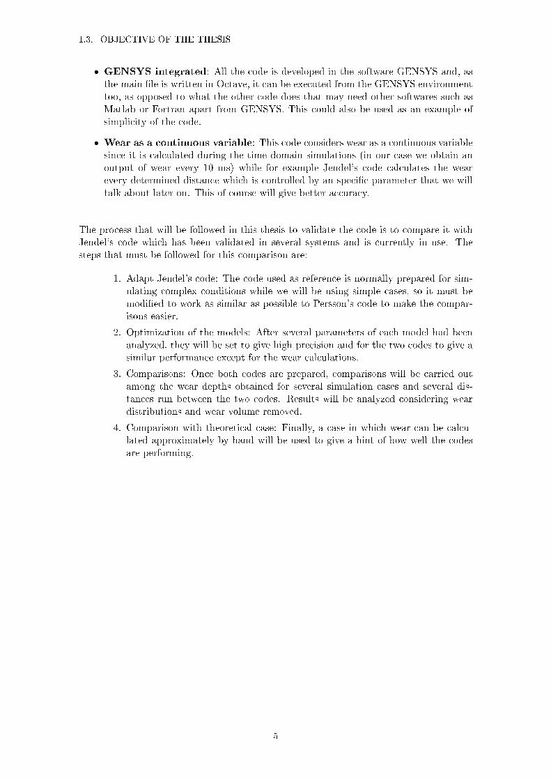
In this chapter the general methodology applied in the models that are in focus of thisthesis is explained. Both Jendel's and Persson's methods are developed in the softwareGENSYS [4] which is a three-dimensional general multi-body-dynamics program. In orderto compare in an easy way, Jendel's code has been modi�ed to be as close as possibleto Persson's code so the structure of these wear prediction codes follow the same stepsuntil they reach the part where the actual wear is calculated. This common methodologyis described here. For the speci�c parts of each part's methodology and to learn aboutJendel's original code, see Chapters 6 and 7. A basic scheme of how these models workcan be seen in Figure 2.1.
Figure 2.1: Chart that represents the general methodology followed by the two modelsanalyzed in this thesis
7

CHAPTER 2. GENERAL METHODOLOGY
Start wheel pro�les
The prediction is done by a series of loops (or wear steps) when a case is simulated ineach one of them. But before entering the loops the original wheel pro�les must be set.
Load simulation model
The data of the simulation model has to be loaded to use as an input. The �lesCalc01.tsimf and vehicle.ins are where this information is stored for Persson's and Jendel'smodels respectively.
All of the characteristics of the vehicle are written in these �les such as masses andinertias of the bodies and characteristics of the suspension system. Track geometry, dis-tances and irregularities (ideal track in our case) are also included in this �le as well asthe type of rail and wheel pro�les. Finally the simulation model also contains the vehiclespeed and the coe�cient of friction used at the wheel-rail contact.
Calculation of wheel-rail geometry functions
Once the simulation enters in the wear loops, the �rst thing to do is to calculate wheel-rail geometry functions. The wheel-rail geometry functions are created in GENSYS by themain program KPF. These fucntions are calculated from designed or measured wheel andrail pro�les. To see an explanation of the wheel-rail geometry functions, see Chapter 4.
Vehicle-track interaction
The vehicle-track interaction is performed in GENSYS by the command and subpro-gram TSIM. TSIM executes the time simulations through numerical integration, in thiscase through the Heun's method.
Wear calculation
When the forces and creepages produced in the contact have been calculated, thegenerated wear is calculated. This is the main di�erence between the two models. Both ofthem are calculated through Archard's law (see Chapter 5) but it's performed in di�erentways.
Post-processing of the wear
The wear obtained is not going to be in the format we want, so it has to be treated. Fil-tering and organization of the wear are some of the things done during the post-processing.Speci�c post-processing methods are explained in Chapters 6 and 7.
Pro�le update
To �nish the wear step, the wheel pro�les must be updated to serve as an input for thenext step. This is as simple as removing the wear depth obtained to the pro�le that hasbeen used in the correspondant step.
8

Chapter 3
Simulation model
In this chapter the model that will be simulated is going to be de�ned. This model isloaded through a TSIM �le in both codes: calc01.tsimf in Persson's code, and throughvehicle.ins in Jendel's code. The attributes of this model that are de�ned in this �le arethe vehicle, the track and other characteristics such as coe�cient of friction, vehicle speed,irregularities and so on.
3.1 Vehicle characteristics
The vehicle used is a passenger vehicle that consists of a single carbody with two bogies,four wheelsets and eight wheels. In the vehicle de�nition, masses, lengths, sti�nesses anddampings of all of the parts are stated as well as the geometry properties of the primaryand secondary suspension. Also local and general systems of coordinates are de�ned withinthis part.
Figure 3.1: Simple scheme of the vehicle used in the simulation
In the code, to identify the di�erent elements of the vehicle a sequence of numbers isused, being the �rst one related to the car (always 1 in our case), the second one relatedto the bogie and the last one depending on which axle of the bogie it is (�rst or second).Also in the case of the wheels a letter is added to di�erentiate between left(l) and right(r).For example wheel 121l would be the left wheel of the �rst wheelset of the second bogie(third wheelset overall).
9
CHAPTER 3. SIMULATION MODEL
3.2 Track geometry
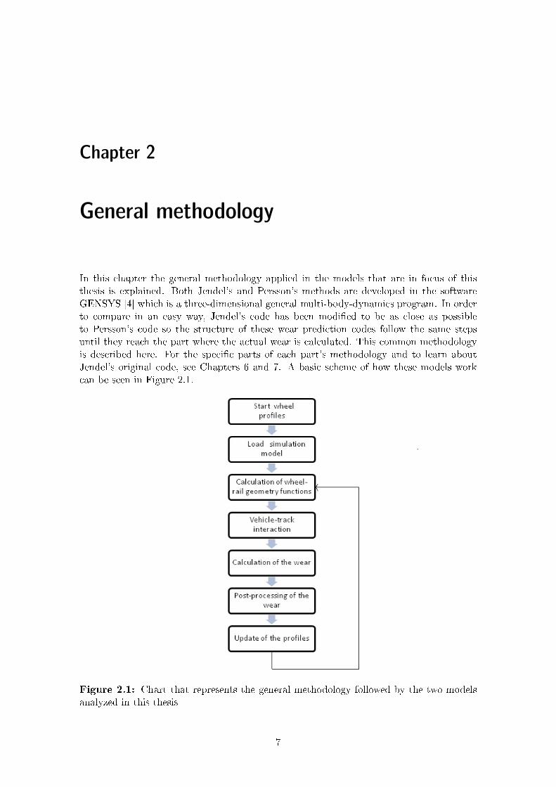
To check that the new wear prediction tool works properly, it must be tried out on severalrepresentative tracks. To cover the di�erent type of tracks we will be using three cases:tangent track, a curve with a radius of R=1000 m and a cant on the outer rail of ht=0.1 mand a curve of R=500 m with a cant on the outer rail of ht=0.15 m. The use of these threecases is also supposed to give us a hint of how the models are performing since we alreadyknow that tangent track should give us small tread wear, while the R=500 m curve caseshould give high wear most of all around the �ange and obviously the R=1000 m curvecase should have a wear in the middle of the two previously mentioned cases.
The distance de�ned for each curve is 280 m. These curve cases are de�ned in a waythat the vehicle enters in the transition curve, stays on the circular curve for some distanceand then �nishes with the �nal transition curve.
Figure 3.2: De�nition of a type curve [5]
The results obtained for wear when making several wear steps can be a little high forthe corresponding conditions. However they are not realistic results, since for exampleif we make 100 wear steps on the R=500 m curve it means that the vehicle makes thiscurve 100 times and in real networks several di�erent types of geometries are mixed, withdi�erent conditions.
3.3 Other important characteristics of the model
Aside from vehicle and track properties there are other parameters or characteristics thatmust be de�ned in the simulation model:
� Vehicle speed: To make easier the comparisons the vehicle will be running at constantspeed. This speed is 150 km/h.
� Track irregularities: In order to eliminate the possibility of some randomness in theresults we will use an ideal track with no irregularities. However we will have to havethis in mind when making the comparisons because the existence of irregularitiestends to homogenize the results (normal distribution), and without them we will beobtaining the same result over and over.
� Coe�cient of friction: The coe�cient of friction is a really important factor in thewheel-rail contact. It depends on the loads that exist in the contact, the slip velocity,the materials of the contact surfaces, etc. If the contact were lubricated this coe�-cient of friction has some variation depending on the sliding velocity. In our case we
10

3.4. SYMMETRIC TRACK
are dealing with non-lubricated contact and we will be always using a coe�cient offriction of 0.5.
� Pro�les: For the comparisons the same normalized wheel and rail pro�les will beused. The rail pro�le is the UIC60 with an inclination of 1:30, and the wheel pro�leis the S1002.
3.4 Symmetric track
The track simulated in this thesis will be studied as symmetric. This is because we considerthat the vehicle negotiates as many left-hand curves as right-hand curves, and that thevehicle runs back and forth (Figures 3.3 and 3.4).
Figure 3.3: Scheme of the symmetric track: the �rst and second wheelsets in one waywill be the fourth and third wheelsets respectively in the way back [5]
With this consideration in mind, instead of making the analysis and the comparisonswheel by wheel, we just deal with two wheels: outer wheels and inner wheels. The outerwheels are the ones of the wheelsets �rst and fourth, while the inner wheels are the onesof the wheelsets second and third. Mathematically this is done by making the average ofeach set of four wheels as previously mentioned.
11

CHAPTER 3. SIMULATION MODEL
Figure 3.4: View of the four wheelsets of the vehicle: outer wheels (black wheels) andinner wheels (white wheels) [5]
12
Chapter 4
Vehicle-track interaction
In this chapter the wheel-rail contact problem will be described and how it is solved withthe present codes. As a summary, this problem can be split in three parts: the calculation ofthe wheel-rail geometry functions, the normal contact problem and the tangential contactproblem. To approach the solution of this problem the Hertz's theory is used. With this,the normal contact problem is partly solved, using the normal force as an input for thetangential contact problem. To face the tangential contact problem Kalker's simpli�edtheory is used.
4.1 Coordinate system
Two main coordinate systems will be used for the solution of the vehicle-track interaction.The �rst one is the coordinate system of the wheel pro�les which is de�ned as an x− y− zsystem with x pointing the longitudinal direction being positive in the travelling directionof the vehicle, y the axis that points the lateral direction de�ned positive towards the �angewheel and z the vertical axis which is positive pointing the upwards direction.
On the other hand a local coordinate system for the contact surface between wheeland rail must be de�ned. This is coordinate system is de�ned as ξ − η − ζ where ξ ispositive in the rolling direction, ζ is perpendicular to the contact surface and η completesthe left handed coordinate system. Creepages and creep forces are de�ned following thiscoordinate system. As the contact surface is di�erent for each wheel it is clear that eachwheel will have its own coordinate system.
13

CHAPTER 4. VEHICLE-TRACK INTERACTION
Figure 4.1: Coordinates systems x − y − z and ξ − η − ζ: Left wheel seen form behind(left) and top view of the contact surface (right) [5]
4.2 Wheel-rail geometry functions
The wheel-rail geometry functions are needed to calculate the contact points at wheels andrails. These mentioned functions are [1],[6]:
� The change in the rolling radius ∆r.
� The contact angle γ.
� The vertical translation of the wheel ∆z.
� Lateral di�erence in curvature between wheel and rail de�ned as:
∆Cy =1
Rry+
1
Rwy(4.1)
14
4.3. NORMAL CONTACT PROBLEM
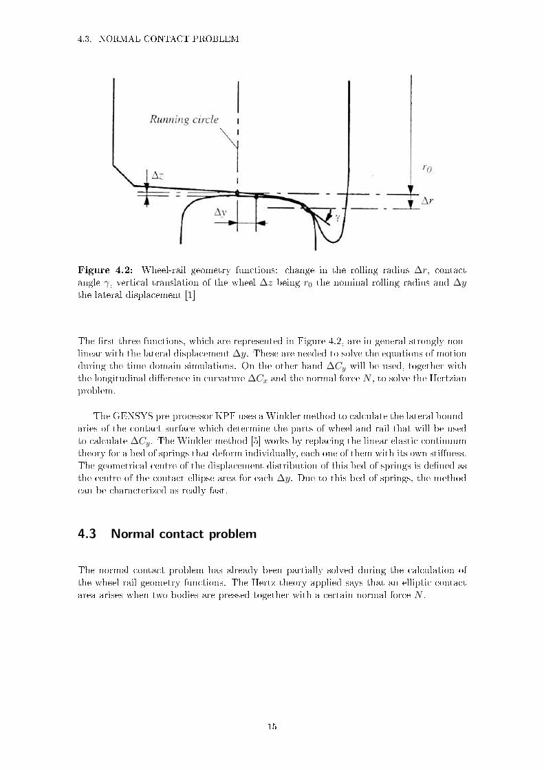
Figure 4.2: Wheel-rail geometry functions: change in the rolling radius ∆r, contactangle γ, vertical translation of the wheel ∆z being r0 the nominal rolling radius and ∆ythe lateral displacement [1]
The �rst three functions, which are represented in Figure 4.2, are in general strongly non-linear with the lateral displacement ∆y. These are needed to solve the equations of motionduring the time domain simulations. On the other hand ∆Cy will be used, together withthe longitudinal di�erence in curvature ∆Cx and the normal force N , to solve the Hertzianproblem.
The GENSYS pre-processor KPF uses a Winkler method to calculate the lateral bound-aries of the contact surface which determine the parts of wheel and rail that will be usedto calculate ∆Cy. The Winkler method [5] works by replacing the linear elastic continuumtheory for a bed of springs that deform individually, each one of them with its own sti�ness.The geometrical centre of the displacement distribution of this bed of springs is de�ned asthe centre of the contact ellipse area for each ∆y. Due to this bed of springs, the methodcan be characterized as really fast.
4.3 Normal contact problem
The normal contact problem has already been partially solved during the calculation ofthe wheel-rail geometry functions. The Hertz theory applied says that an elliptic contactarea arises when two bodies are pressed together with a certain normal force N .
15

CHAPTER 4. VEHICLE-TRACK INTERACTION
Figure 4.3: Elliptical contact patch with semi-axes length a and b [5]
This theory works under some assumptions:
� The half-space assumption: The contact patch is small compared to typical bodysurfaces such that wheel and rail can be assumed as semi-in�nite bodies limited bya plane.
� In the near contact surface, curvatures of the bodies are considered as constant.
� The surface roughness is neglected.
� The bodies consist of homogeneous, linear and elastic materials.
� Only elastic displacements and strains are considered.
� As a consequence of the half-space assumption and the bodies having the same elasticproperties, the problem can be de�ned as quasi-identical, which allows the separationof the problem into normal and tangential contact problems.
Even though it is said that half-space assumption is not valid when �ange contact occursbecause the lateral wheel pro�le radius in the �ange is in the same range as the size of thecontact patch, Hertz's theory is the major tool to solve contact problems in rail vehicledynamics since non-Hertzian methods are much more time consuming.
From the application of the Winkler method the centre point of the ellipse contact areahas been located, so now the length of the ellipse's semi-axes a and b, must be found. Thesemi-axes are functions of the wheel radius both in longitudinal and lateral direction, therail radius in longitudinal direction, the rail head radius in lateral direction, the normalforce and material properties such as Young's modulus and Poisson's ratio. However forgiven wheel and rail pro�les these semi-axes can be tabulated before the simulations forrelative lateral displacements between rail and wheel.
4.4 Tangential contact problem
Now the solution to the tangential problem must be found. This consists of determiningthe creep forces. The creepages are de�ned by normalizing the components of the sliding
16
4.4. TANGENTIAL CONTACT PROBLEM
velocity between the vehicle speed as follows:
υξ =vξ
vvehicle(4.2)
υη =vη
vvehicle(4.3)
φ =w
vvehicle(4.4)
where:
υξ,υη are the longitudinal and lateral creepages respectively (-)φ is the spin creepage (1/m)
vξ,vη are the longitudinal and lateral components of the sliding velocity (m/s)w is the angular velocity(1/s)
vvehicle is the vehicle speed (m/s)
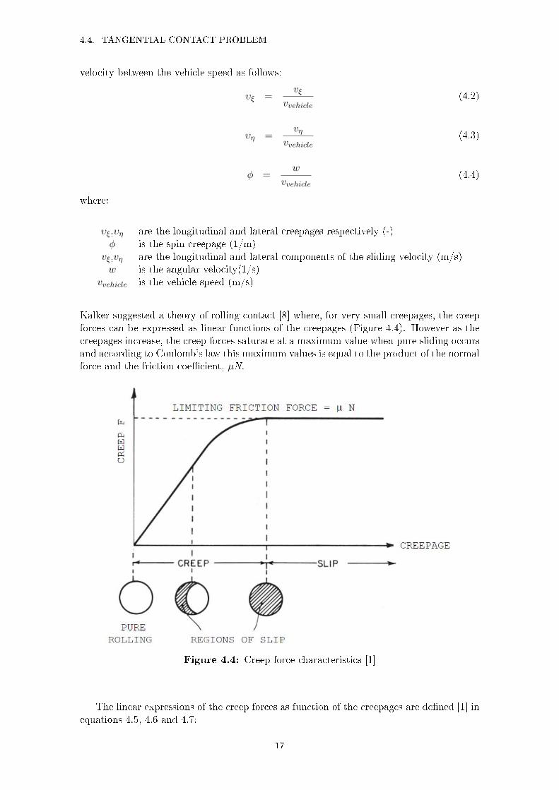
Kalker suggested a theory of rolling contact [8] where, for very small creepages, the creepforces can be expressed as linear functions of the creepages (Figure 4.4). However as thecreepages increase, the creep forces saturate at a maximum value when pure sliding occursand according to Coulomb's law this maximum values is equal to the product of the normalforce and the friction coe�cient, µN.
Figure 4.4: Creep force characteristics [1]
The linear expressions of the creep forces as function of the creepages are de�ned [1] inequations 4.5, 4.6 and 4.7:
17

CHAPTER 4. VEHICLE-TRACK INTERACTION
Fξ = −c2GC11υξ (4.5)
Fη = −c2GC22υη − c3GC23φ (4.6)
Mφ = −c3GC32υη − c4GC33υξ (4.7)
where:
c=√
ab where a and b are the lengths of the contact
patch ellipse semi-axes (m)Fξ,Fη are the longitudinal and lateral creep forces
respectively exerted on the wheel body (N)Mφ is the moment exerted around the perpendicular (Nm)
direction to the contact patch (Nm)vξ,vη are the longitudinal and lateral components of the
sliding velocity (m/s)G is the shear modulus (N/m2)Cij The creepage and spin coe�cients which are
dependant of the ratio a/b and the Poisson's ratioυξ,υη are the longitudinal and lateral creepages respectively (-)φ is the spin creepage (1/m)
However the linear theory cannot be used for wear calculations since it assumes thatthere is no slip, which is needed to calculate the wear. To solve this problem, Kalker createdan algorithm called FASTSIM which works only over Hertzian areas since the coe�cientsCij of the linear theory, which upon FASTISM is based on, are just tabulated for Hertzianareas. Apart from calculating frictional stresses according to Kalker's simpli�ed theory, itis also used as a post-processor to determine the division of the contact area into adhesionand slip zones. The tangential solution is just calculated for the output data time stepsform the vehicle-track simulations, not for each time step, so it doesn't represent too muchmore simulation time.
The contact ellipse is divided into cells and when each of these cells results in a tangen-tial stress that overcomes the limit imposed by the coe�cient of friction times the Hertziancontact pressure according to Figure 4.5, slip occurs.
18

4.4. TANGENTIAL CONTACT PROBLEM
Figure 4.5: De�nition of parameters in the contact ellipse [6]
To perform the wear calculations according to Chapter 5, the slip velocity must befound for each cell. This slip velocity vector follows equation 4.8:
vslip = vvehicle · [(υξ − φ · η, υη + φ · ξ) − δ
δξ(uξ, uη)] (4.8)
where:
ξ, η are the local coordinates in the surface area (m)φ is the spin creepage (1/m)
vξ,vη are the longitudinal and lateral components of the sliding velocity (m/s)uξ,uη are the components of the elastic displacement vector of the surface (m)vvehicle is the vehicle speed (m/s)
The elastic slip term (last term of equation 4.8) is disregarded as the rigid terms are muchlarger. Finally the sliding distance for each cell can be calculated multiplying the slipvelocity by the step time, which is also determined by the relation between vehicle speedand local longitudinal displacement.
∆s=vslip∆t ∆t=∆ξ vvehicle (4.9)
19


Chapter 5
Wear calculations
The next step after having calculated the wheel-rail geometry functions and simulating thevehicle-track interaction, is to calculate the wear. To do that, Archard's wear law is used[1] [2]. Archard's wear law states that wear volume is directly proportional to normal load,sliding distance and a constant, and inversely proportional to the hardness of the material.
Vwear = kNs
H(5.1)
where:
Vwear is the volume wear removed (m3)N is the normal load (N)s is the sliding distance (m)k is the constant called wear coe�cient (-)H is the hardness of the material (N/m2)
The wear coe�cient k, is determined through a wear map (Figure 5.1) depending on twoquatities: the contact pressure and the sliding velocity.
21

CHAPTER 5. WEAR CALCULATIONS
Figure 5.1: Wear map, where the wear coe�cient is a function of the sliding velocity andthe contact pressure [5]
As the Hertzian theory is used, the contact pressure can be calculated as follows [4](N/m2) :
p(ξ, η) =3N
2πab
√1 − (
ξ
a)2 − (
η
b)2 (5.2)
where ξ and η are the local coordinates of the contact patch.
Obviously the k2 region belongs more to tread contact as it usually has lower slidingvelocities, while the rest of the regions belong to the �ange contact where the highest forcesare produced. Even though we use ideal conditions, it is important to point out that withdi�erent conditions such as lubrication, braking situation or di�erent types of weather aswell as the use of worn pro�les, the wear coe�cient must be multiplied by some factorsthat have been previously tabulated.
5.1 Wear calculations of Jendel’s model
In Jendel's model the wear depth normal to the contact surface is obtained as an output ofthe wear calculations. This is because Archard's wear law is adapted to calculate directlythe wear depth [5] for each cell of the contact patch considering that volume wear can beexpressed as Vwear = ∆ξ∆η∆ζ and that the area of each cell is ∆A = ∆ξ∆η.
Vwear = kp∆A∆s
H(5.3)
Therefore the wear depth (m) perpendicular to the contact surface can be de�ned as:
22

5.2. WEAR CALCULATIONS OF PERSSON'S MODEL
∆ζ = kp∆s
H(5.4)
where ∆s (m) is the sliding distance of an element of the contact patch, k the wearcoe�cient, H the hardness of the material (N/m2), and p the contact pressure (N/m2).
5.2 Wear calculations of Persson’s model
In Persson's model Archard wear law is also modi�ed but to obtain wear volume rate (m3/s)[4] instead of wear volume (m3) . Wear depth is obtained later during the post-processing(section 7.1.1).
Vwear = kNvslipH
(5.5)
In order to obtain volume wear rate instead of volume wear, just sliding distance has beenreplaced by sliding velocity. This means that in Persson's model sliding velocity doesn'tneed to be integrated.
5.3 Example of wheel wear
In Figure 5.2 an example of the shape of wear produced on the outer wheels (whelsets 1and 4) after running 28 km on the R=500 m curve is shown along the wheel pro�les beforeand after running that distance.
23

CHAPTER 5. WEAR CALCULATIONS
−40 −20 0 20 40
0
10
20 Pro�le beforePro�le after
−40 −20 0 20 400
0.1
0.2
0.3
Figure 5.2: Example of wear depth: Pro�les before and after wear (Top) and wear depth(Bottom). After running 28 km on the R=500 m curve with Persson's model. Numbersare in mm.
On the horizontal axis of the Figure 5.2, the position on the wheel is shown, where the�ange is positioned in the positive values. That is why at the positive values the highestpeak of wear occurs since the highest values of the contact forces and sliding speeds areproduced there. The other two peaks on the tread exist around 20 and -20 mm. The peaksof the tread correspond to contact point 1 while the peak on the �ange corresponds tocontact point 2.
24

Chapter 6
Reference code: T.Jendel’s model
The model that will be used as a reference to see if the new model works properly is theone developed by Thomas Jendel. To perform the comparisons easier, Jendel's code hasto be modi�ed so it is as similar as possible to the new model.
As said before, Jendel's code follows the general methodology explained in Chapter2 until it reaches the part of the wear calculations. Nevertheless in the present chapterwe will give a brief explanation of how this model works, which modi�cations had to bedone before making the comparisons and �nally we will proceed to analyze some of theparameters accessible to the user that can modify the performance of the code.
6.1 Methodology
T. Jendel's model is originally prepared for simulating several tracks at a time with di�erentcurve radius discretizations and complex conditions such as lubrication, worn pro�les,several types of irregularities, coe�cients of friction and so on. The execution of the codeis carried out by �le wp6_cc.m which is a MATLAB �le and it also loads an input �lecalled inputv7.m that contains other model characteristics. The �ow chart of Jendel's codeis presented in Figure 6.1.
25

CHAPTER 6. REFERENCE CODE: T.JENDEL'S MODEL
Figure 6.1: Flow chart of the reference wear prediction tool [5]
At the beginning of wp6_cc.m a parameter dy must be de�ned by the user to knowin how many rings the width of the wheels will be discretized. Obviously, the smaller dyvalues, more points of the wheel will be taken into account and more precision is supposedto be obtained.
In the original Jendel's code [5],to de�ne the track geometry in the time domain simu-lations, an S matrix is de�ned, which stores a simulation in each row and a characteristicof the track in each column such as number of rail pro�les, the number of coe�cient offriction, number of rail pro�les, etc. Once the wheel-rail contact geometry calculations aredone, and the vehicle-track interaction is simulated, wear calculations are performed withthe help of a software programmed in FORTRAN (aside form MATLAB) because, this isfaster when it comes to �for� loops. To perform the wear calculations, the discretization ofthe contact patch must be selected by the user through parameters m and n. However thiswear calculations are not performed every time step, but they are calculated every speci�cdistance which is set through parameter L_sample that it is available for the user. It hasbeen stated that the value 2πr0 (being r0 the rolling radius of the wheel) for L_sample isconsidered good enough to predict wear reference. If we choose, in our simulation model,an L_sample of 2πr0, the number of calculations that will be performed for each wheel inone simulation step (280 m) can be de�ned as:
Number of wear calculations =280
2πr0= 89 (6.1)
26

6.1. METHODOLOGY
89 wear calculations will thus be performed along the 280 m of simulated track duringone step of simulation. As said in Chapter 1, wear is not a continuous variable and if wewould like to approach its behaviour to a continuous one, L_sample should be reduced asmuch as possible. Back in the MATLAB environment, the wear depths obtained must beweighted. This means that as several tracks had been simulated at a time, the wear mustbe weighted depending on how much distance has been run in each track. To do that �rstof all we have to calculate the total real simulated distance for each radius curve intervalsince several simulations can be carried out for one interval in each wear step [6].
Lsimreal,i = Ni2πr0
L_sampleLsim,i (6.2)
where Lsimreal,i is the total real simulated distance, Ni the number of simulations in theinterval i and Lsim,i the total simulated distance for the interval i. With this distance theweighted wear ww,i(y) can be easily obtained through equation 6.3:
ww,i(y) =Ltot,i
Lsimreal,iwi(y) (6.3)
being Ltot,i the total track length of all the curves in the interval and wi(y) the wear fromthe simulations of the curve radius interval i correspondent to Lsimreal,i.
After the vectors of wear depths are weighted, both the resulting vector and the pro�lesmust be smoothed. This is done with splines, which perform an interpolation with cubicfunctions over the signals. The last step for this model is to update the pro�les. In orderto update the pro�les, both horizontal and vertical coordinates of the pro�le are changedconsidering the contact angle γ since the wear obtained is perpendicular to the contactsurface, accordng to equations 6.4 and 6.5:
y_updated = y − wwearstep(y) · sin(γ) (6.4)
z_updated = z − wwearstep(y) · cos(γ) (6.5)
6.1.1 Modifications of Jendel’s code
As previously said, comparisons between the two models will be easier if they are as similaras possible and that the only parts that remain di�erent are the ones related to the wearcalculations and post-processing of this wear. These modi�cations are:
� Simulation model: Instead of de�ning the simulation conditions through the �leLOADTRACK.m, our simulation model is going to be loaded through a �le calledvehicle.ins. This �le is nearly identical to the one that will be used in I.Persson'scode. However in Persson's code the contact model is de�ned through functionwr_coupl_pra3 of GENSYS in the TSIM �le, in order to be able to perform thewear calculations in GENSYS, while in Jendel's the contact model used to calculatethe creep forces de�ned through function wr_coupl_pe3 is outside this TSIM �le.This means that some of the characteristics of the contact models are de�ned in adi�erent way and in a di�erent place, so to set them to the same value in both codescan be a di�cult task.
27

CHAPTER 6. REFERENCE CODE: T.JENDEL'S MODEL
� Common parameters: Obviously, to make both codes as similar as possible, commonparameters such as sti�nesses, masses, dampings, coe�cients of friction and so onshould be set to the same values. As the TSIM �le used is nearly the same in bothcodes we will just have to focus on the magnitudes that are de�ned in the contactmodel wr_coupl_pra3 of Persson's code, trying to identify where they are in Jendel'scode and set them to the same value.
� Weighted calculations: As in the simulation model of this thesis just one track at atime is simulated, it doesn't make sense to weight the wear. That is why we removedthe weighted calculation performed in wp6_cc.m and replace them by the simpleaverage of the four outer wheels and the simple average of the four inner wheels.
� Smoothing: The smoothing that is carried out by splines will be replaced by thesame second order �lter that is used in Persson's code to eliminate the possibility ofobtaining di�erent results because of having a di�erent �lter in both codes.
6.2 Results and discussion
In this section we will proceed to the analysis of the parameters of the code (after themodi�cations) that can change the results obtained when these are modi�ed. All the pa-rameters that are going to be studied in this section belong to the main �le wp6_cc.m.The �rst parameter to check is the discretization of the width of the wheel dy. After thatthe number of samples that are going to be taken during the wear calculations, L_sample,should also be taken into account. In order to perform the wear calculations, the con-tact ellipse must be discretized into cells. The number of these cells is controlled by theparameters m and n which are also and object of study in this part.
6.2.1 Discretization of the width of the wheel, dy
The discretization of the width of the wheels, which is controlled through the parameterdy, sets the number of points of the lateral direction of the wheel that will be used. Asall discretizations, with smaller intervals a more accurate result should be obtained. Herethe maximum interval length is set to 0.1 mm because if not numerical errors may happenduring the calculations of the wheel-rail geometry functions. The values of dy that havebeen simulated are 0.025 mm, 0.0125 mm, 0.00625 mm and the standard value of 0.05mm. Several wear distributions obtained for the outer wheels after running 28 km on theR=500 m curve can be found in Figure 6.2:
28

6.2. RESULTS AND DISCUSSION
Figure 6.2: Wear depth of the outer wheels after running 28 km for the case of R=500m curve with di�erent dy lengths
In terms of wear distribution it can be seen that only around the peaks of the �angesome variations can be seen, however there is not a clear trend of pattern for these vari-ations. The bigger variations are produced in �ange contact because this is where thechanges in wear are bigger from one position to another. Therefore if the intervals are toobig, the interpolation between the wear results does not give such a good result. On theother hand, the lateral distribution of the wear is identical for all the cases. If we check howthese changes on the peaks a�ect the total volume removed (Table 6.1) we observe thatthe amount of material removed doesn't change so much (biggest change around 6.5%).
dy R=500 m ; ht=0.15 m R=1000 m ; ht=0.1 m
0.05 mm 8.7214e-006 m3 4.0539e-006 m3
0.025 mm 8.3770e-006 m3 4.0577e-006 m3
0.0125 mm 8.1557e-006 m3 4.0589e-006 m3
0.00625 mm 8.3065e-006 m3 4.0601e-006 m3
Table 6.1: Total volume removed from the outer wheel for the cases of R=500 m curveand R=1000 m curve with di�erent dy lengths after running 28 km
Simulation time is not clearly a�ected by the change in the discretization of the widthof the wheel as can be concluded from the results shown in Table 6.2.
29

CHAPTER 6. REFERENCE CODE: T.JENDEL'S MODEL
dy R=500 m ; ht=0.15 m R=1000 m ; ht=0.1 m
0.05 mm 1h 37 min 1h 54 min
0.025 mm 1h 53 min 1h 58 min
0.0125 mm 1h 50 min 1h 48 min
0.00625 mm 1h 57 min 1h 56 min
Table 6.2: Simulation time for the cases of R=500 m curve and R=1000 m curve withdi�erent dy lengths after running 28 km
It can be concluded that the discretization of the width of the wheel is not such a de-terminant parameter, neither in terms of wear distribution nor in computational e�ciency.Thus the standard value of 0.05 mm can be considered as good enough.
6.2.2 Sampling of the wear calculations, L_sample
As previously said, the number of wear calculations performed over a certain simulateddistance is controlled through parameter L_sample. When analyzing this parameter itjust makes sense to study lower values than the standard one, so the e�ect on the outputcan be seen when the model approaches the behaviour of the wear to a continuous onegiving a result closer to reality. The values simulated aside from the standard one are0.628m (5 times smaller) and 0.314m (10 times smaller).
Figure 6.3: Wear depth of the outer wheels after running 28 km for the case of R=500m curve with di�erent L_sample numbers
In Figure 6.3 the e�ect of varying the sampling distance over the wear distribution isclear at the peaks of the �ange. An appreciable change occurs when the sampling distance
30

6.2. RESULTS AND DISCUSSION
is reduced from 3.14 m to 5 times smaller (0.628 m), while between 0.628 m and 0.314 mthe di�erence is negligible. This is also occurs when we speak about total volume removed(Table 6.3) even though the change is not so big (maximum around 6%).
L_sample R=500 m ; ht=0.15 m R=1000 m ; ht=0.1 m
3.14 m 8.7214e-006 m3 4.0539e-006 m3
0.628 m 8.2085e-006 m3 4.0569e-006 m3
0.314 m 8.3269e-006 m3 4.0556e-006 m3
Table 6.3: Total volume removed from the outer wheel for the cases of R=500 m curveand R=1000 m curve with di�erent sampling distances after running 28 km
For comparison purposes, decreasing this parameter is interesting apart from beingmore accurate, because it also eliminates the possibility of obtaining di�erent results be-tween the two codes because of having di�erent number of samples taken. However, inTable 6.4 we can see that decreasing the sampling distance is a big threat to the simula-tion time too as it increases too much. That is why in practical cases 3.14 m should beused as the standard sampling distance.
L_sample R=500 m ; ht=0.15 m R=1000 m ; ht=0.1 m
3.14 m 1h 37 min 1h 54 min
0.628 m 5h 4 min 4h 47 min
0.314 m 5h 33min 6h 18 min
Table 6.4: Simulation time for the cases of R=500 m curve and R=1000 m curve withdi�erent sampling distances after running 28 km
6.2.3 Discretization of the contact ellipse, m and n
During wear calculations the discretization of the contact patch must be chosen in the �lewp6_cc.m. The size of these cells are governed by the parameters m and n. The originalvalues for this parameters are 50 for each of them. The only reasonable simulations to tryare with higher values (so bigger discretization) to take into account more points of thecontact patch, always increasing the two parameters at the same time to have a smootherresult. Aside from the standard one, two discretizations have been simulated: 75x75 and100x100.
31
CHAPTER 6. REFERENCE CODE: T.JENDEL'S MODEL
Figure 6.4: Wear depth of the outer wheels after running 28 km for the case of R=500m curve with di�erent m and n numbers
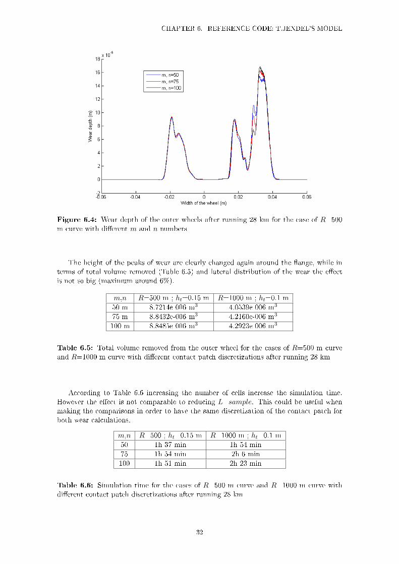
The height of the peaks of wear are clearly changed again around the �ange, while interms of total volume removed (Table 6.5) and lateral distribution of the wear the e�ectis not so big (maximum around 6%).
m,n R=500 m ; ht=0.15 m R=1000 m ; ht=0.1 m
50 m 8.7214e-006 m3 4.0539e-006 m3
75 m 8.8432e-006 m3 4.2160e-006 m3
100 m 8.8485e-006 m3 4.2923e-006 m3
Table 6.5: Total volume removed from the outer wheel for the cases of R=500 m curveand R=1000 m curve with di�erent contact patch discretizations after running 28 km
According to Table 6.6 increasing the number of cells increase the simulation time.However the e�ect is not comparable to reducing L_sample. This could be useful whenmaking the comparisons in order to have the same discretization of the contact patch forboth wear calculations.
m,n R=500 ; ht=0.15 m R=1000 m ; ht=0.1 m
50 1h 37 min 1h 54 min
75 1h 54 min 2h 6 min
100 1h 51 min 2h 23 min
Table 6.6: Simulation time for the cases of R=500 m curve and R=1000 m curve withdi�erent contact patch discretizations after running 28 km
32

Chapter 7
Code to validate: I.Persson’s model
The code developed by Ingemar Persson is the object of validation of this thesis. Thee�orts on establishing a new tool for the calculation of the wear of the railway vehicle'swheels are motivated because of several advantages that this model can give in comparisonto Jendel's model, speci�cally in comparison to the model that is treated here as reference.
In this chapter we will study the speci�c methodology of this new model and the analysisof the parameters that can be changed by the user and that can modify the output.
7.1 Methodology
The structure of Persson's model uses the methodology described in Chapter 2 so thedi�erences with Jendel's methodology will be explained here. The main di�erence betweenthese structures are the wear calculation process and how they post-process the obtainedwear from Archard's law. The code is MATLAB based and can be executed through eitherMATLAB or Octave. The �ow chart of the wear calculation program wear_loop.m can beseen in the chart 7.1.
33

CHAPTER 7. CODE TO VALIDATE: I.PERSSON'S MODEL
Figure 7.1: Flow chart of the new wear calculation code
As can be seen the wear calculations are included inside the vehicle-track interactionsimulations. In order to do that inside the dynamic simulation a new function calledwr_coupl_pra3 is de�ned. It is similar to wr_coupl_pe3, which is called in the simulationmodel of Jendel's code to calculate the creep forces through FASTSIM. This new function,apart from calculating the creep forces, also includes Archard's law to calculate the weardirectly and that is why wear can be calculated every time step (approximately continuousbehaviour). Meanwhile Jendel's code has to calculate creepages and creep forces accordingto some values already tabulated, post-process the contact patch in Matlab and discretizeit to calculate the contact pressures and sliding speeds of all of the elements.
As explained in Chapter 5, in Persson's code Archard's law is applied in a way thatvolume wear rate is obtained instead of volume.
7.1.1 Post-processing
The post-processing in Persson's code is carried out by the �le wear.mplotf which belongs tothe block MPLOT of GENSYS. The task of this post-processing is to translate the outputof function wr_coupl_pra3 into wear depth distribution along the lateral coordinate ofthe wheel. This post-processing can be split in several steps:
Statistical analysis:
A statistical analysis is used to place the volume wear rate along the width of thewheels. It is carried out by function Stat2 [4]. There are 8 variables accessible for the
34
7.1. METHODOLOGY
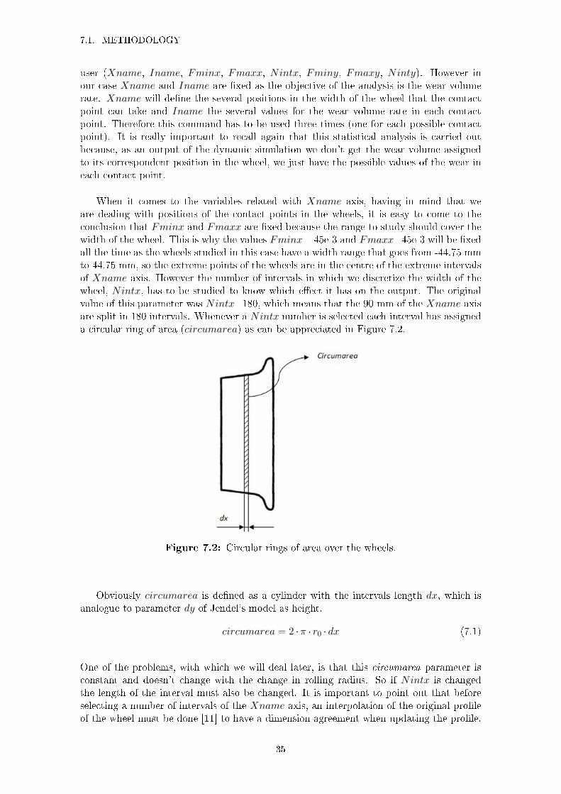
user (Xname, Iname, Fminx, Fmaxx, Nintx, Fminy, Fmaxy, Ninty). However inour case Xname and Iname are �xed as the objective of the analysis is the wear volumerate. Xname will de�ne the several positions in the width of the wheel that the contactpoint can take and Iname the several values for the wear volume rate in each contactpoint. Therefore this command has to be used three times (one for each possible contactpoint). It is really important to recall again that this statistical analysis is carried outbecause, as an output of the dynamic simulation we don't get the wear volume assignedto its correspondent position in the wheel, we just have the possible values of the wear ineach contact point.
When it comes to the variables related with Xname axis, having in mind that weare dealing with positions of the contact points in the wheels, it is easy to come to theconclusion that Fminx and Fmaxx are �xed because the range to study should cover thewidth of the wheel. This is why the values Fminx=-45e-3 and Fmaxx=45e-3 will be �xedall the time as the wheels studied in this case have a width range that goes from -44.75 mmto 44.75 mm, so the extreme points of the wheels are in the centre of the extreme intervalsof Xname axis. However the number of intervals in which we discretize the width of thewheel, Nintx, has to be studied to know which e�ect it has on the output. The originalvalue of this parameter was Nintx=180, which means that the 90 mm of the Xname axisare split in 180 intervals. Whenever a Nintx number is selected each interval has assigneda circular ring of area (circumarea) as can be appreciated in Figure 7.2.
Figure 7.2: Circular rings of area over the wheels.
Obviously circumarea is de�ned as a cylinder with the intervals length dx, which isanalogue to parameter dy of Jendel's model as height.
circumarea = 2 ·π · r0 · dx (7.1)
One of the problems, with which we will deal later, is that this circumarea parameter isconstant and doesn't change with the change in rolling radius. So if Nintx is changedthe length of the interval must also be changed. It is important to point out that beforeselecting a number of intervals of the Xname axis, an interpolation of the original pro�leof the wheel must be done [11] to have a dimension agreement when updating the pro�le.
35

CHAPTER 7. CODE TO VALIDATE: I.PERSSON'S MODEL
The reason is that the wear will have the dimension according the new Nintx while theoriginal pro�le will have the one corresponding Nintx of the last simulation performed.
When it comes to the possible values of the wear rate represented by Iname axis, theparameters are analogous to the ones de�ned in the Xname axis. The limits of this axis areset by Fminy and Fmaxy. Fminy must be set negative in a way that the �rst intervalis symmetric to zero, so the values between Fminy and -Fminy are assigned to zero.Meanwhile the upper limit of the Iname axis, Fmaxy, must be picked high enough toconsider all of the wear rate values obtained. All wear rate values higher than Fmaxy willbe cut o� from the statistical analysis. The problem is that the higher this value is, morestatistical analysis must be done which will imply longer simulation time, so when selectingthis value the user must have a sense of the order of magnitude of the possible volume wearrates that will be obtained. Once the range of the axis is picked the user should select inhow many intervals it is going to be split, which is done through the parameter Ninty.Obviously when we increase Ninty, accuracy increases as the considered interval is smaller.
Once the input parameters to the command Stat2 are selected, the statistical analysisis performed according to Figure 7.3:
Figure 7.3: Display of how Stat2 works
The output is presented divided in cells (given in per mille), in each of which is storedthe probability of a combination between a certain Xname with a certain Iname, havingXname in the horizontal axis and Iname in the vertical one. Both of the axis, Xnameand Iname, go from a minimum value Fminx and Fminy respectively to a maximumvalue Fmaxx and Fminy (end level of the last intervals), divided in the middle by stepsde�ned by the expressions 7.2 and 7.3:
dx =(Fmaxx− Fminx)
Nintx(7.2)
36
7.1. METHODOLOGY
dy =(Fmaxy − Fminy)
Ninty − 1(7.3)
Finally as outputs the X-curve de�ned by the centre point of each column and theY-curve de�ned by Equation 7.4, are obtained.
Y − curvei =n∑j=1
Probability(Xnamei, Inamej) · Inamej (7.4)
This curve represents the volume wear rate (m3/s) placed along the width of wheel.
Filtering the signal:
The �ltering is carried out by function lpass2 which applies an spatial �lter to thevolume wear rate (m3/s) obtained. Two variables have to be introduced as input, the signalto �lter and a vector with the positions. This will smooth the signal without disregardingimportant information. After the �ltering the wear vector is reversed and a second �lteringis applied in order to eliminate the possible phase shift when �ltering. After this second�ltering, the vector is reversed again to get the original pro�le, �ltered twice and with nophase shift.
Calculation of wear depth:
To calculate wear depth (m) from volume wear rate (m3/s), �rst volume wear (m3)must be obtained. This is done by multiplying the output of Stat2 (once it has been�ltered) by the corresponding simulation time.
cpa_XwArchSplin1 = cpa_XwArchSplin · simulation_time (7.5)
being cpa_XwArchSplin1 the vector of volume wear of the wheel X, while the vector ofvolume wear rate of the wheel X is cpa_XwArchSplin.
Finally this volume wear vector must be divided by the previously mentioned parameter(circumarea), which represents the total area of the wheel in order to obtain wear depth.
cpa_XwArchDepth =cpa_XwArchSplin1
circumarea(7.6)
where cpa_XwArchDepth represents the vector of wear depths of the wheel X.
Nevertheless according to the de�nition of circumarea, it represents the area of acylinder, so it is neglecting the change of rolling radius that occurs along the width of thewheel. This approximation can be considered good around the thread. However aroundthe �ange, it is something to have in mind when the comparisons are done since the changein contact angle is not negligible and might a�ect the results.
The post-processing is supposed to just organize the wear along the width of the wheelbut it alters the amount of volume wear removed (Table 7.1).
37

CHAPTER 7. CODE TO VALIDATE: I.PERSSON'S MODEL
R=500 m ; ht=0.15 m R=1000 m ; ht=0.1 m
before Stat2 6.7459e-008 m3 3.7738e-008 m3
after Stat2 7.0690e-008 m3 3.9104e-008 m3
Table 7.1: Total amount of wear volume removed before and after the application ofStat2
This e�ect has to be taken into account when performing the comparisons. Once thepost-processing is done, the average of the four outer wheels is performed, as well as theaverage of the four inner wheels, taking into account the symmetry conditions mentionedin Chapter 3.
7.2 Results and discussion
In order to comprehend how this code works, it is essential to know which of the wearparameters can modify the output in a considerable way, and then try to understand howthey work. The parameters of this code that will be analyzed are i) the number of intervalsin which we discretizise both the Xname and Iname axis of the Stat2 function and ii) thenumber of cells in which the contact patch is dicretizised, m and n.
7.2.1 Number of intervals of the Xname axis, Nintx
To see the e�ect of this parameter we are going to use a discretization with four number ofintervals Nintx=359, Nintx=717, Nintx=1433 and the standrad one of Nintx=180 forthe curves of R=500 m and R=1000 m .The results of the wear depth for the outer wheelsafter running 5.6 km are shown in Figure 7.4.
38

7.2. RESULTS AND DISCUSSION
Figure 7.4: Wear depth of the outer wheels after running 5.6 km for the case of R=500m curve with di�erent Nintx numbers
It is clearly appreciated that the wear distribution is not signi�cantly a�ected by theincrease of the number of intervals. Besides that, when total volume removed and simula-tion time are checked it doesn't seem that Nintx is such an important parameter for theresult obtained at the output of the post-processing.
Nintx R=500 m ; ht=0.15 m R=1000 m ; ht=0.1 m
180 1.5014e-006 m3 6.1919e-007 m3
359 1.5331e-006 m3 6.1840e-007 m3
717 1.5167e-006 m3 6.1869e-007 m3
1433 1.4829e-006 m3 6.0639e-007 m3
Table 7.2: Total volume removed from the outer wheel for the cases of R=500 m curveand R=1000 m curve with di�erent Nintx numbers after running 5.6 km
Nintx R=500 m ; ht=0.15 m R=1000 m ; ht=0.1 m
180 59 min 42 min
359 1h 2 min 47 min
717 48 min 38 min
1433 1h 7 min 51 min
Table 7.3: Simulation time for the cases of R=500 m curve and R=1000 m curve withdi�erent Nintx numbers after running 5.6 km
Nevertheless for comparison purposes it is interesting to increase this parameter, sinceit is analogous to the dy parameter of Jendel's. Besides that, the standard value of the
39

CHAPTER 7. CODE TO VALIDATE: I.PERSSON'S MODEL
length of the intervals in Persson's code (dx=0.5 mm) is 10 times bigger than in Jendel'scode (dy=0.05 mm), therefore increasing Nintx we reduce dx.
7.2.2 Number of intervals of the Iname axis, Ninty
The values for the number of intervals in which the Iname axis is discretized areNinty=4002(standard), Ninty=8003, Ninty=16005 and Ninty=32009. It must be pointed out thatthese numbers are quite big because the upper limit of the axis, Fmaxy, has been setreally high to assure that none value of wear is cut o� from the statistical analysis. Inpractical cases this upper limit should be studied to minimize simulation time withoutlosing accuracy.
Figure 7.5: Wear depth of the outer wheels after running 5.6 km for the case of R=500m curve with di�erent Ninty numbers
In Figure 7.5 it is clear that there are really small discrepancies around the higher peakof the �ange. In terms of the total volume removed (Table 7.4) the trend seems to decreasebeing the maximum discrepancy of 9% which is considerable. Meanwhile, the behaviour ofsimulation time (Table 7.5) is not so clear and it really depends on how large is the rangeof the Iname axis.
Ninty R=500 m ; ht=0.15 m R=1000 m ; ht=0.1 m
4002 1.5014e-006 m3 6.1919e-007 m3
8003 1.4727e-006 m3 6.1253e-007 m3
16005 1.4788e-006 m3 6.0194e-007 m3
32009 1.3684e-006 m3 5.9329e-007 m3
Table 7.4: Total volume removed from the outer wheel for the cases of R=500 m curveand R=1000 m curve with di�erent Ninty numbers after running 5.6 km
40

7.2. RESULTS AND DISCUSSION
Ninty R=500 m ; ht=0.15 m R=1000 m ; ht=0.1 m
4002 59 min 42 min
8003 1h 2 min 50 min
16005 1h 9 min 34 min
32009 1h 1 min 49 min
Table 7.5: Simulation time for the cases of R=500 m curve and R=1000 m curve withdi�erent Ninty numbers after running 5.6 km
It can be concluded that Ninty is an important parameter to increase since it has aconsiderable e�ect in total volume removed with the advantage of not increasing too muchthe simulation time if the upper limit of Iname is not excessively high.
An important fact to recall when selecting Ninty are the cases in which really smallwear values are produced. If Ninty is not high enough, volume wear rate can end up intothe �rst interval so the statistical analysis will identify them as zero wear. To �x thisNinty must be increased until the interval's length dy is small enough to detect the wear.As an example, in the tangent track case after running 28 km where the wear produced isconsiderably smaller when the number of intervals is set to 51 (Figure 7.6), the only thingthat can be appreciated is noise. On the other hand, when Ninty is increased up to 13056(Figure 7.7) a clear peak of wear appears on the tread.
Figure 7.6: Wear depth of the outer wheels after running 28 km on tangent track withNinty=51
41

CHAPTER 7. CODE TO VALIDATE: I.PERSSON'S MODEL
Figure 7.7: Wear depth of the outer wheels after running 28 km on tangent track withNinty=13056
7.2.3 Discretization of the contact patch, m and n parameters
These parameters have the same function as in Jendel's code: they discretizise the contactpatch in cells. As it was stated in Chapter 6 the bigger the values of m and n, the moreaccurate results we are going to obtain since more points of the contact patch are takeninto account.
Three discretizations are used: the standard of 16x16 and then 25x25 and 40x40. Thedi�erent wear distributions of the outer wheels when increasing these parameters for thecase of R=500 m after running 5.6 km are presented in Figure 7.8.
42

7.2. RESULTS AND DISCUSSION
Figure 7.8: Wear depth of the outer wheels after running 5.6 km for the case of R=500m curve with di�erent m and n numbers
At �rst sight it can appreciated that the positions of the peaks tend to change whenincreasing the number of cells of the contact patch. However, the location of the wear alongthe width of the wheel is consistent. This change translated into volume wear reveals anincreasing trend when more points of the contact patch are considered (up to a 14%).
m,n R=500 m ; ht=0.15 m R=1000 m ; ht=0.1 m
16 1.5014e-006 m3 6.1919e-007 m3
25 1.5667e-006 m3 6.6676e-007 m3
40 1.5910e-006 m3 7.1286e-007 m3
Table 7.6: Total volume removed from the outer wheel for the cases of R=500 m curveand R=1000 m curve with di�erent m and n numbers after running 5.6 km
With this, we can conclude that m and n are decisive parameters in order to obtainmore precision in the wear calculations since it has a relevant e�ect on the amount ofmaterial removed. The drawback is that according to Table 7.7 it a�ects computationale�ciency, so the user must �nd a good compromise between the precision he/she needs,and the available simulation time.
43

CHAPTER 7. CODE TO VALIDATE: I.PERSSON'S MODEL
m,n R=500 m ; ht=0.15 m R=1000 m ; ht=0.1 m
16 59 min 42 min
25 1h 21 min 48 min
40 1h 55 min 1h 12 min
Table 7.7: Simulation time for the cases of R=500 m curve and R=1000 m curve withdi�erent m and n numbers after running 5.6 km
44
Chapter 8
Comparisons
Once Jendel's code has been properly adapted to work as similar as possible to Persson'scode, and that the analysis of the parameters available for the user that can modify theoutput has been carried out, it is time to make the comparisons between the two models.It will start with a comparison of the two models in order to ensure that their dynamicbehaviour is similar. Then we will compare the results for the wear distributions withdi�erent running distances and the discrepancies are explained. Finally a theoretical casewill be described and the results of the comparison between this case and the two modelsare presented.
8.1 Comparison of the dynamic behaviour
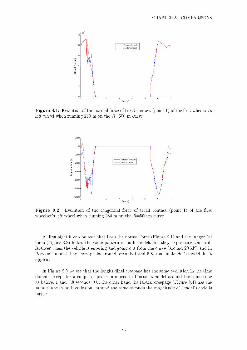
In order to see if the modi�cations performed of Jendel's code have e�ectively made bothmodels behave similar dynamically speaking, some key quantities are compared. The keyquatities that are of importance from a wear analysis point of view are the ones extractedfrom Archard's wear law. That is why normal wheel-rail force is one of the parameters toanalyze as well as both the longitudinal and the lateral creepages since they are directlyrelated to sliding velocity. Also the resulting tangential force is studied to have moreinformation about the dynamic behaviour.
The comparisons are performed for the left wheel of the �rst wheelset since it is theone that is exposed to the hardest conditions: guidance with two contact points (�angecontact). Speci�cally the results shown in the �gures below correspond to the tread contactpoint (contact point 1) for the case of R=500 m curve.
45
CHAPTER 8. COMPARISONS
Figure 8.1: Evolution of the normal force of tread contact (point 1) of the �rst wheelset'sleft wheel when running 280 m on the R=500 m curve
Figure 8.2: Evolution of the tangential force of tread contact (point 1) of the �rstwheelset's left wheel when running 280 m on the R=500 m curve
At �rst sight it can be seen that both the normal force (Figure 8.1) and the tangentialforce (Figure 8.2) follow the same pattern in both models but they experience some dif-ferences when the vehicle is entering and going out from the curve (around 20 kN) and inPersson's model they show peaks around seconds 1 and 5.8, that in Jendel's model don'tappear.
In Figure 8.3 we see that the longitudinal creepage has the same evolution in the timedomain except for a couple of peaks produced in Persson's model around the same timeas before, 1 and 5.8 seconds. On the other hand the lateral creepage (Figure 8.4) has thesame shape in both codes but around the same seconds the magnitude of Jendel's code isbigger.
46
8.1. COMPARISON OF THE DYNAMIC BEHAVIOUR
Figure 8.3: Evolution of the longitudinal creepage of tread contact (point 1) of the �rstwheelset's left wheel when running 280 m on the R=500 m curve
Figure 8.4: Evolution of the lateral creepage of tread contact (point 1) of the �rstwheelset's left wheel when running 280 m on the R=500 m curve
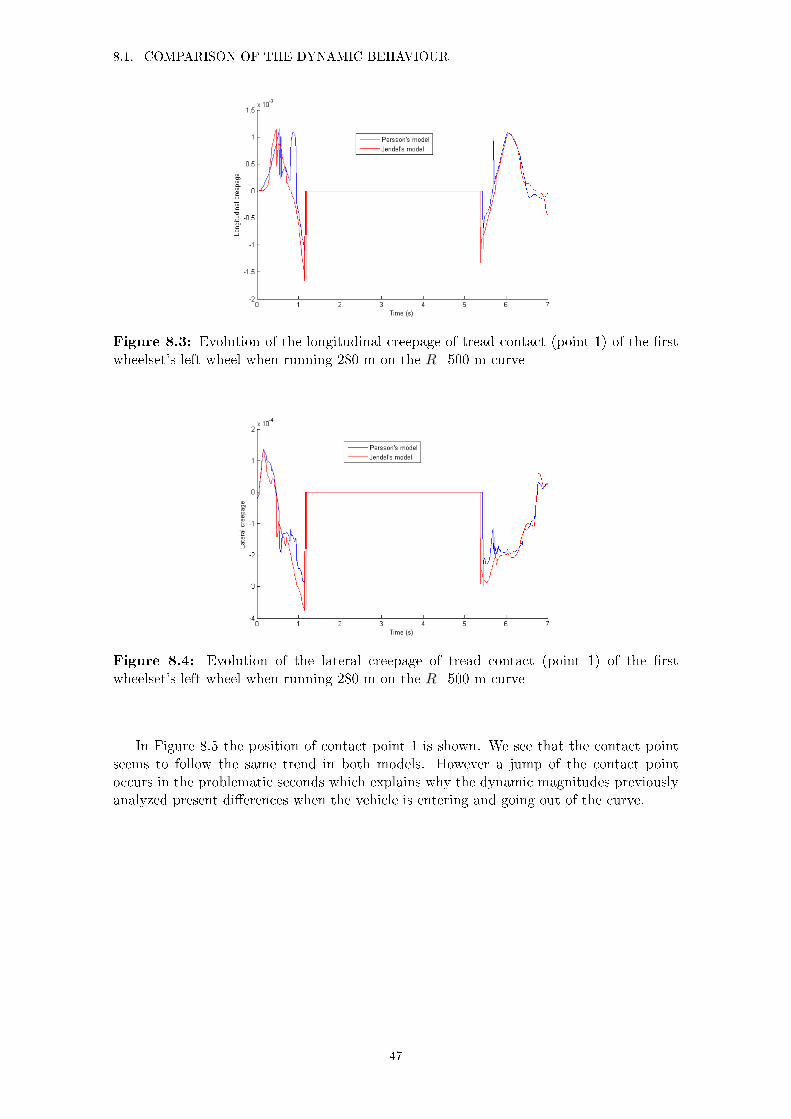
In Figure 8.5 the position of contact point 1 is shown. We see that the contact pointseems to follow the same trend in both models. However a jump of the contact pointoccurs in the problematic seconds which explains why the dynamic magnitudes previouslyanalyzed present di�erences when the vehicle is entering and going out of the curve.
47
CHAPTER 8. COMPARISONS
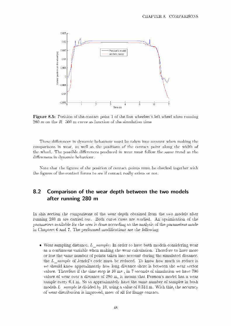
Figure 8.5: Position of the contact point 1 of the �rst wheelset's left wheel when running280 m on the R=500 m curve as function of the simulation time
These di�erences in dynamic behaviour must be taken into account when making thecomparisons in wear, as well as the positions of the contact point along the width ofthe wheel. The possible di�erences produced in wear must follow the same trend as thedi�erences in dynamic behaviour.
Note that the �gures of the position of contact points must be checked together withthe �gures of the contact forces to see if contact really exists or not.
8.2 Comparison of the wear depth between the two modelsafter running 280 m
In this section the comparisons of the wear depth obtained from the two models afterrunning 280 m are carried out. Both curve cases are studied. An optimization of theparameters available for the user is done according to the analysis of the parameters madein Chapters 6 and 7. The performed modi�cations are the following:
� Wear sampling distance, L_sample: In order to have both models considering wearas a continuous variable when making the wear calculation. Therefore to have moreor less the same number of points taken into account during the simulated distance,the L_sample of Jendel's code must be reduced. To know how much to reduce itwe should know approximately how long distance there is between the wear vectorvalues. Therefore if the time step is 10 ms , in 7 seconds of simulation we have 700values of wear over a distance of 280 m, it means that Persson's model has a wearsample every 0.4 m. So to approximately have the same number of samples in bothmodels L_sample is divided by 10, using a value of 0.314 m. With this, the accuracyof wear distribution is improved, most of all for �ange contact.
48

8.2. COMPARISON OF THE WEAR DEPTH BETWEEN THE TWO MODELS AFTER
RUNNING 280 M
� Discretization on the statistical analysis: Parameters Ninty and Nintx, which setthe number of intervals in which the axes of function Stat2 are discretized, haveshown to have some e�ect on how the wear is distributed, especially Ninty. Thatis why both of them are increased. The upper limit of the vertical axis of Stat2has been set to 300e-9 m3/s, using a number of intervals of 1205 which means aninterval length of dy=0.25e-9 m3/s . On the other hand, as Nintx is an analogousparameter to the parameter dy of Jendel's code that has a value of 0.05 mm, thenumber of intervals of the horizontal axis is increased up to 1433 so the intervallength is dx=0.0625 mm. With this change, the wear is better organized and moreprecision is obtained.
� Discretization of the contact patch: It has been stated from previous chapters thatthe discretization of the contact ellipse (parameters m and n) has an important e�ectover the obtained wear. We can set the same discretization for the wear calculations.We use a discretization of 40x40 that is the maximum available for Persson's code.
After performing the comparisons, conclusions are extracted regarding wear distribu-tion and total amount of wear removed.
8.2.1 R=500 m curve case
The comparison of the wear depth for the case of R=500 m curve can be found in Figure8.6.
Figure 8.6: Wear depth of the outer wheels for both models after running 280 m on theR=500 m curve
At �rst sight discrepancies are seen in the peak of wear that is around 0.02 m, andmost of all in the peaks of �ange contact which are probably produced at the wheels of theouter rail of the curve where �ange contact happens. To understand better the di�erencesin wear distribution on the outer wheels (average of wheels 111l, 111r, 122l, 122r) we lookat Appendix B where the comparisons wheel by wheel after running 280 m are presented.
49

CHAPTER 8. COMPARISONS
In the R=500 m curve case the wheels in which the discrepancies previously mentionedoccur are the two wheels of the outer rail that corresponds to the outer wheels (111l,122l).We will study the contact points 1 (tread contact) and 2 (�ange contact), and the normalforces produced over these points.
Figure 8.7: Evolution of the normal forces of contact points 1 and 2 of wheel 111l in bothmodels
Figure 8.8: Evolution of the position relative to the nominal running circle of contactpoints 1 and 2 of wheel 111l in both models
Wheel 111l is responsible for the peaks of the �ange. In Figures 8.7 and 8.8 we seethat the normal forces and the positions of the contact points �t quite well except for someoscillation of the normal force of Persson's model around the interval 0.5s-1s. Persson'smodel is neglecting the change in rolling radius so in the �ange it is considering a smallerarea, therefore it is obtaining a bigger wear depth. We can appreciate that in Jendel'smodel the peaks are lower and wider, while in Persson's model the peaks are higher andmore abrupt. This is produced because of the jump of the contact point 1 and it is alsothe cause of oscillation of the rest of the quantities.
Meanwhile, wheel 122l also takes part in �ange contact as well as in the peak of weararound 0.02 m. The peak produced in the �ange in wheel 122l in Persson's model is muchhigher than in Jendel's model. This makes sense since the normal force produced over
50
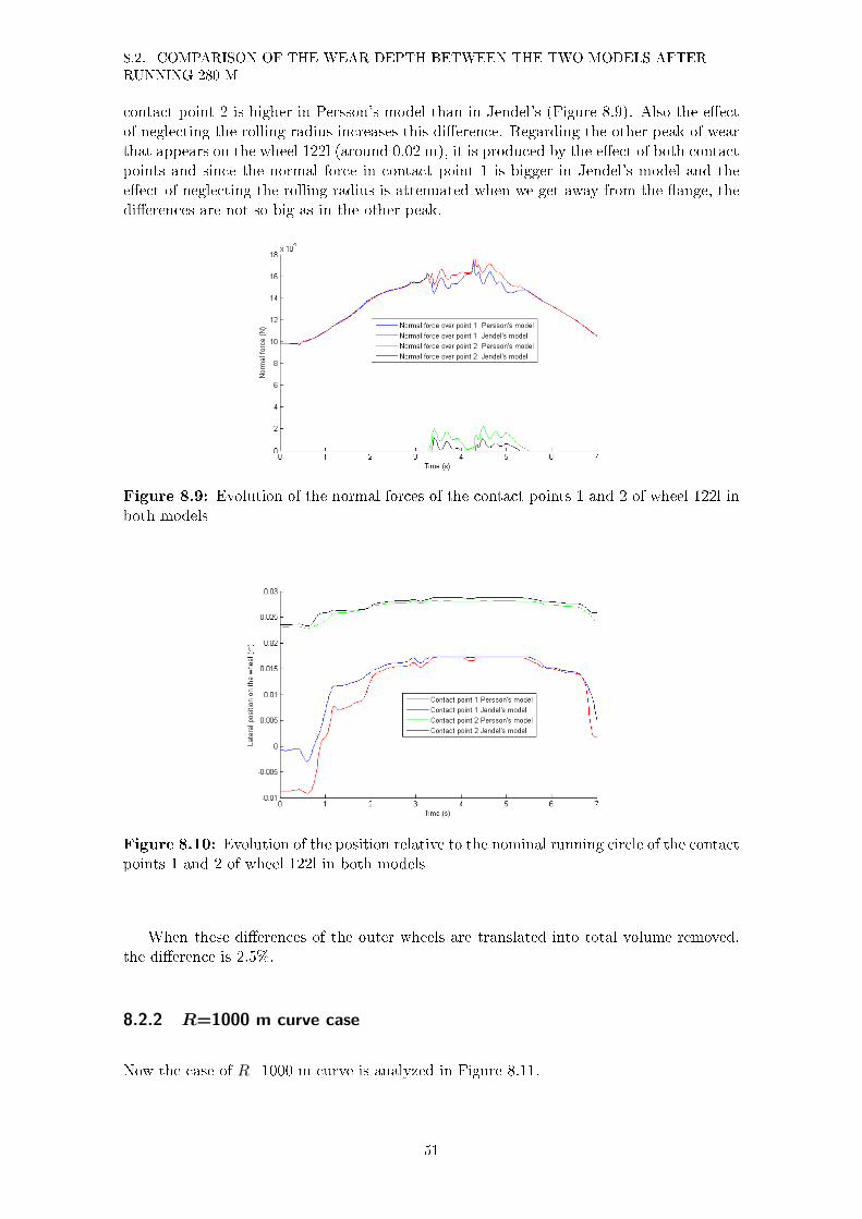
8.2. COMPARISON OF THE WEAR DEPTH BETWEEN THE TWO MODELS AFTER
RUNNING 280 M
contact point 2 is higher in Persson's model than in Jendel's (Figure 8.9). Also the e�ectof neglecting the rolling radius increases this di�erence. Regarding the other peak of wearthat appears on the wheel 122l (around 0.02 m), it is produced by the e�ect of both contactpoints and since the normal force in contact point 1 is bigger in Jendel's model and thee�ect of neglecting the rolling radius is attenuated when we get away from the �ange, thedi�erences are not so big as in the other peak.
Figure 8.9: Evolution of the normal forces of the contact points 1 and 2 of wheel 122l inboth models
Figure 8.10: Evolution of the position relative to the nominal running circle of the contactpoints 1 and 2 of wheel 122l in both models
When these di�erences of the outer wheels are translated into total volume removed,the di�erence is 2.5%.
8.2.2 R=1000 m curve case
Now the case of R=1000 m curve is analyzed in Figure 8.11.
51

CHAPTER 8. COMPARISONS
Figure 8.11: Wear depth of the outer wheels for both models when running 280 m onthe R=1000 m curve
The di�erences in wear distribution are found in the �ange and in the peak of weararound 0.02 m. The wheels 111l and 122l must be checked again for this case, being wheel111l responsible for �ange contact and wheel 122l responsible for the peak of wear around0.02 m.
In Appendix B we see that on the wheel 111l there are two appreciable peaks of wearon the �ange, being the highest peak related to the contact point 2 while the other one isrelated to both contact points.
Figure 8.12: Evolution of the normal forces of contact points 1 and 2 of wheel 111l inboth models
52

8.2. COMPARISON OF THE WEAR DEPTH BETWEEN THE TWO MODELS AFTER
RUNNING 280 M
Figure 8.13: Evolution of the position relative to the nominal running circle of the contactpoints 1 and 2 of wheel 111l in both models
We see (Figure 8.13) that around 1.7s and 4.8s a jump produced in contact point 1on Persson's model makes the normal load go from contact point 2 to contact point 1(Figure 8.12). At these instants the normal force of Jendel's model exceeds the normalforce of Persson's model (around 20 kN) and that is why the peak of wear in Jendel'smodel is bigger. In this case, these di�erences are somehow reduced because of neglectingthe change in rolling radius in Persson's model (it has the opposite e�ect as before).
On the other hand the second peak is also a�ected by contact point 1, so the di�erencesin normal forces on the seconds 1.7s and 4.8s are compensated between the two contacts(Figure 8.12). Nevertheless, as the transition of the contact point 2 from one peak toanother is smoother in Jendel's model, it has less wear in this second peak while it hasmore wear in the middle of the peaks compared to Persson's.
When it comes to wheel 122l (Figures 8.14 and 8.15), there is a clear peak that is alittle displaced between the two models but with a similar magnitude.
Figure 8.14: Evolution of the normal forces of contact points 1 and 2 of wheel 122l inboth models
53
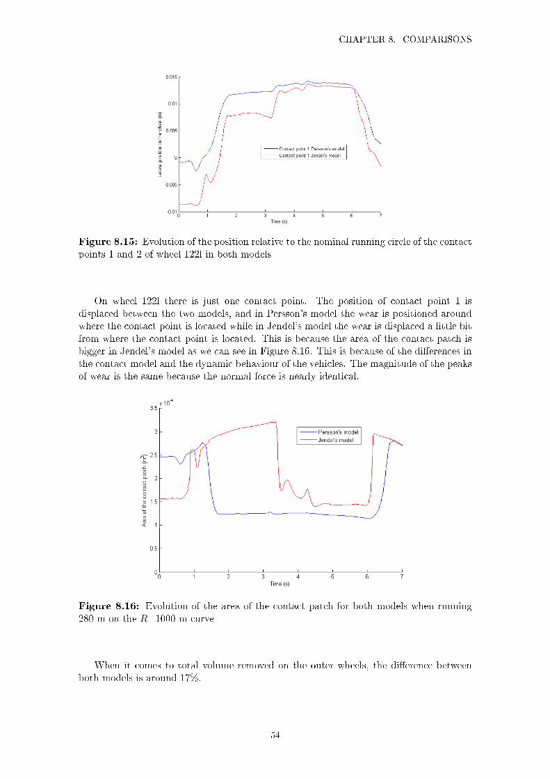
CHAPTER 8. COMPARISONS
Figure 8.15: Evolution of the position relative to the nominal running circle of the contactpoints 1 and 2 of wheel 122l in both models
On wheel 122l there is just one contact point. The position of contact point 1 isdisplaced between the two models, and in Persson's model the wear is positioned aroundwhere the contact point is located while in Jendel's model the wear is displaced a little bitfrom where the contact point is located. This is because the area of the contact patch isbigger in Jendel's model as we can see in Figure 8.16. This is because of the di�erences inthe contact model and the dynamic behaviour of the vehicles. The magnitude of the peaksof wear is the same because the normal force is nearly identical.
Figure 8.16: Evolution of the area of the contact patch for both models when running280 m on the R=1000 m curve
When it comes to total volume removed on the outer wheels, the di�erence betweenboth models is around 17%.
54

8.3. COMPARISON OF THE WEAR DEPTH BETWEEN THE TWO MODELS AFTER
RUNNING 5.6 KM
8.3 Comparison of the wear depth between the two modelsafter running 5.6 km
In this section we can see how the di�erences between the two models evolve with increasedrunning distance. In order to make of this a more practical case, the sampling distanceis increased to its original value and the discretization of the contact patch of Persson'smodel is reduced from 40x40 to 24x24. This way, when simulating 5.6 km, the simulationtime goes down by 42.5% for Persson's model and by 74% for Jendel's model.
The wear depth distribution for the outer wheels after running 5.6 km on the R=500m and R=1000 m curves can be found in Figures 8.17 and 8.18:
Figure 8.17: Wear depth of the outer wheels for both models after running 5.6 km onthe R=500 m curve
Figure 8.18: Wear depth of the outer wheels for both models after running 5.6 km onthe R=1000 m curve
We see that the di�erences in wear distribution don't increase so much when the runningdistance increases. In terms of volume removed with respect to the previous section, the
55

CHAPTER 8. COMPARISONS
di�erence in removed volume between the two models has gone up from 2.5% to 10% inthe R=500 m curve, and from a 17% to a 26% in the R=1000 m curve.
8.4 Comparison with the theoretical case
Finally, the models are compared with a theoretical case. The wear volume rate obtainedwith this calculation will be compared with the output of the Archard's wear law used inPersson's code. Also the di�erences in total volume removed between the two models andthe theoretical case are checked.
8.4.1 Methodology
To make the wear calculations by hand, we need that the whole contact patch is sliding. Inthis way there is no need for a discretization between adhesion and sliding and Equation5.5 can be directly applied. Material's hardness is a constant value and the normal forceis obtained as an output from the simulations. Meanwhile sliding velocity is determinedaccording to Equation 4.8 as the creepages are also obtained in the simulation and thewear coe�cient is clearly k2 since we are dealing with tread contact.
In order to achieve sliding conditions, running on tangent track at 150 km/h, constraintsare set for the pitch velocity of the �rst and second wheelsets. Then overspeed is manuallyapplied on the �rst wheelset, while underspeed is set on the second wheelset using thefollowing equations:
Overspeed = −(100 + l
100)vvehicler0
(8.1)
Underspeed = −(100 − l
100)vvehicler0
(8.2)
where r0 is the rolling radius, vvehicle the vehicle speed (m/s) and l the percentage of slidingto apply.
10% and 25% sliding are used to assure that total sliding occurs. First wheelset's leftwheel, which is the critical one, will be the one to analyze.
8.4.2 Results and discussion
In Figures 8.19 and 8.20 the results for 10% sliding and 25% sliding are presented, wherethe comparisons between the wear rate obtained with Persson's model and the one obtainedby hand appear.
56

8.4. COMPARISON WITH THE THEORETICAL CASE
Figure 8.19: Wear volume rate of wheel 111l obtained with 10% sliding
Figure 8.20: Wear volume rate of wheel 111l obtained with 25% sliding
It can be appreciated that for both cases the results of wear volume rate are quite close,so it can be said that Persson's model is performing the wear calculations correctly. Totranslate this into numbers and to compare them also with Jendel's model we use totalwear volume removed. The results are presented in Table 8.1:
57
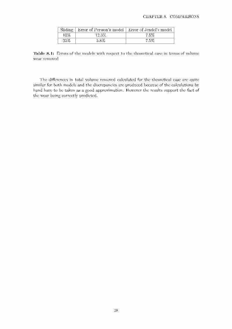
CHAPTER 8. COMPARISONS
Sliding Error of Persson's model Error of Jendel's model
10% 12.5% 7.5%
25% 5.8% 7.5%
Table 8.1: Errors of the models with respect to the theoretical case in terms of volumewear removed
The di�erences in total volume removed calculated for the theoretical case are quitesimilar for both models and the discrepancies are produced because of the calculations byhand have to be taken as a good approximation. However the results support the fact ofthe wear being correctly predicted.
58

Chapter 9
Conclusions and future work
In this chapter the conclusions extracted from this thesis are listed, as well as the severalthings which the future work should be focused on, in terms of the performance of themodel and other ways of validation.
First of all, Persson's model represents an improvement in terms of the ease of dealingwith the code, when it comes to understanding and modifying it. The fact that everythingis done in GENSYS clari�es the structure of the model, and allows GENSYS users to usethis wear prediction tool.
An analysis of the parameters, available for the user to choose, that can modify theoutputs is carried out for both models. When it comes to the parameters of Persson'smodel some conclusions can be extracted. The discretization of the contact patch shouldbe carefully selected taking into account simulation time. This discretization has a directe�ect on the total amount of wear obtained by Archard's law. However 24x24 discretizationcan be assumed as a good compromise between simulation time and accuracy of the weardistribution.
The other parameters of the code to validate that have to be set by the user belongto the post-processing. The key part of this post-processing is the statistical analysis per-formed over the results obtained from Archard's law. This statistical analysis is performedusing two axis: the horizontal axis (lateral position of the contact points) and the verticalaxis(wear volume rate values). From the horizontal axis the limits of the axis must be setsuch as the extreme points of the width of the wheel that is object of study, are in themiddle of the extreme intervals. Meanwhile the number of intervals of this horizontal axisis not such a determinant parameter and as a reference it can be used the same length ofintervals that Jendel's uses, 0.05 mm. For the vertical axis, the lower limit must be pickedas negative such as the �rst interval is symmetric to zero and the upper limit, must bechosen high enough to obtain all the possible values of wear obtained from Archard's lawbut not excessively high because the time would increase too much due to the statisticalanalysis that should be performed. The number of intervals of this axis, has a consider-able e�ect on wear distribution and should be increased to obtain more precision, and thesimulation time is not an issue if the upper limit has been set correctly.
Also from the post-processing when wear depth is obtained by dividing volume wearby area of the wheel, this area is assumed to be a cylinder with the radius equal to the
59

CHAPTER 9. CONCLUSIONS AND FUTURE WORK
nominal rolling radius. This is not a good hypothesis when we are dealing with �angecontact. So in �ange contact more wear than the real one is obtained.
It is important to point out that this post-processing just translates the wear ob-tained from Archard's law into the wear depth distributed along the width of the wheel.Meanwhile the discretization of the contact patch previously mentioned alters the resultsobtained from Archard's law as well as the calculation of the creep forces.
When both codes are compared, it was �rst proven that despite the e�orts of tryingto make both models perform equally dynamically, still some slight di�erences in termsof magnitude (not shape) of variables such as contact forces and creepages occur due tothe contact models being di�erently de�ned in the simulation model. The comparisonsbetween the two models have revealed that their wear predictions are in the same orderof magnitude. Tread wear prediction is nearly identical for the two models, however dif-ferences are manifested when we approach the �ange. This �ange wear follows a similarshape in terms of number of peaks and proportion between them in both models, butthey are a little displaced from one to another and the heights of the peaks are di�erent.These discrepancies can be explained through the di�erences in the dynamic behaviourbetween both models together with alteration of the wear during the post-processing madein Persson's model, so we can say that Persson's model predicts the evolution of the wearaccurately. Besides that, in real cases track irregularities exist, which would homogenizethe results (normal distribution) for both models when several simulations are performed.
Also during the comparison process it was noticed that the peaks of wear of Persson'smodel tend to be sharper and thinner, while the ones of Jendel's are smoother and widerwhich we conclude can be partly explained because the contact points seemed to jumpmore abruptly from one location to another in Persson's model while in Jendel's they havea smoother trajectory.
Perssons's model is also more sensitive to noise when it comes to detect this minor wear(tangent track) and the post-processing parameters should be carefully selected.
Once these conclusions have been extracted, we can think of several things to do forPersson's model as future work:
� As we said, the change in rolling radius is neglected when considering the area togo from volume wear to wear depth. This constant area (circumarea) should bereplaced by a vector that contains the correspondent area for each lateral positionon the wheel.
� The statistical analysis carried out by Stat2 alters the volume wear rate obtained. Amultiplication by a factor should be used to let the wear volume rate obtained afterthe post-processing as the value obtained from Archard's law.
� The peaks of wear depth obtained for Persson's model were sharp and thinner somaybe the signal should be more �ltered.
� The next steps for this model should be preparing the code to simulate more complexconditions such as di�erent types of tracks at the same time, lubrication conditions,braking situations and so on, as well as the prediction of rail wear.
� Finally the model should be compared with �eld measurements from a real line to�nish the validation process.
60

Bibliography
[1] Andersson E, Berg M and Stichel S: Rail vehicle dynamics, Division of Rail Vehicles, De-partment of Aeronautical and Vehicle Engineering, Royal Institute of Technology (KTH),Stockholm 2007.
[2] Archard J F: Contact and rubbing of �at surfaces, Journal of Applied Physics, Vol 24,pp 981-988, 1953.
[3] Chudzikiewicz A and Kalker J J: Wheel-rail wear calculations with the FASTSIM rou-tine, The Archives of Transport, Vol 1, No 1-2, 1989.
[4] DEsolver: GENSYS users manual, GENSYS.1304
[5] Dirks B: Vehicle Dynamics Simulation of Wheel Wear for Swedish High Speed TrainX2000, Report TRITA AVE 2003:16, MSc Thesis, Division of Railway Technology, De-partment of Aeronautical and Vehicle Engineering, Royal Institute of Technology (KTH),Stockholm 2003.
[6] Jendel T: Prediction of wheel pro�le wear-methodology and veri�cation, Licentiate The-sis, TRITA FKT 2000:49, Division of Railway Technology, Department of Vehicle Engi-neering, Royal Institute of Technology (KTH), Stockholm 2000.
[7] Kalker J J: Simulation of the development of railway wheel pro�le through wear, Wear150, pp 355-365, 1991.
[8] Kalker J J: Three-Dimensional Elastic Bodies in Rolling Contact, Kluwer AcademicPublisher, Dordrecht 1990.
[9] Kalker J J and Chudzikiewicz A: Calculation of the evolution of the form of a railwaywheel pro�le through wear, International Series of Numerical Mathematics, Vol. 101, pp71-81, 1991.
[10] Lehna H: Experimental investigations of wear characteristics of technical dry rolling/slidingsystems, Proc. 3rd Int. Conf. on Contact Mechanics and Wear of Rail/Wheel Systems,July 22-26, 1990.
[11] Matlab R2013a , www.mathworks.com/products/matlab
61

BIBLIOGRAPHY
[12] Ward A, Lewis R and Dwyer-Joyce R S: Incorporating a railway wheel wear model intomulti-body simulations of wheelset dynamics, Tribology Series 41:367-376, DepartmentofMechanical Engineering, University of She�eld, She�eld 2002.
62
Appendix A
Notations
Latin letters:
a Longitudinal semi-axis of contact ellipse (m)A Contact area (mm2)b Lateral semi-axis of contact ellipse (m)b0 Half of the track width (m)C Proportionality constant (µg/Nmm)circumarea Area of a ring with lenght dx and radius r0cpa_XwArchDepth Vector of wear depths (Persson's model) (m)cpa_XwArchSplin Vector of wear volume rates (Persson's model) (m3/s)cpa_XwArchSplin1 Vector of wear volume (Persson's model) (m3)Cij Creepage and spin coe�cients (-)∆Cx Longitudinal di�erence in curvature between wheel and rail (1/m)∆Cy Lateral di�erence in curvature between wheel and rail (1/m)d Sliding distance (m)dx Length of intervals of Xname axis (m)dy Length of intervals of Iname axis (m)dy Length of intervals of the width of the wheel (Jendel's model)(m)Fmaxx Upper limit of Xname axis (m)Fmaxy Upper limit of Iname axis (m3/s)Fminx Lower limit of Xname axis (m)Fminy Lower limit of Iname axis (m3/s)Fξ Longitudinal creep force (N)Fη Lateral creep force (N)G Shear modulus (N/m2)H Material surface hardness (N/m2)ht Cant (m)hf Flange height (m)i Curve radius interval (-)k Wear coe�cient in Archard's wear model (-)ke Wear coe�cient in energy wear model, worn mass (µg/Nm)
63
APPENDIX A. NOTATIONS
kw Wear coe�cient in energy model, worn volume (m2/N)l Percentage of slidingL_sample Sample distance from vehicle-track simulations (m)Lsim, i Total simulated track length for all four wheel positions for curve radius interval iLsimreal, i Real simulated distance for curve radius interval i (m)Ltot Total track length (for the entire railway network) (m)Ltot, i Total track length for curve radius interval i (m)Mφ Spin moment (Nm)m Parameter of discretization of the contact patchN Normal force (N)n Parameter of discretization of the contact patchNi Number of simulations for curve radius interval i (-)Nintx Number of intervals of Xname axisNinty Number of intervals of Iname axisp Contact pressure (N/m2)qR Flange inclination measure (m)R Curve radius in circular part (m)Rwy Lateral radius of wheel pro�le (m)Rry Lateral radius of rail pro�le (m)r Wheel rolling radius (m)r0 Wheel rolling radius in running circle (m)∆r Change in rolling radius (m)S Simulation matrixs Sliding distance (m)∆s Magnitude of sliding distance for an element (m)tf Flange thickness (m)∆t The time a contact surface element is in contact (s)T Tangential traction force (N)u Elastic displacement vector in contact surface (m)Vwear Volume of wear (m3)vslip Slip velocity vector (m/s)vvehicle Vehicle speed (km/h)vξ Longitudinal sliding velocity (m/s)vη Lateral sliding velocity (m/s)w(y) Perpendicular wear distribution for a sample in Jendel's model (m)wi(y) Total perpendicular wear distribution for curve radius interval i (m)wwearstep Final wear distribution for a wear step in Jendel's model (m)ww,i Total weighted perpendicular wear distribution for curve radius interval i (m)Wfrictional Frictional work (N mm)WDcell Wear depth per cell (mm)x, y, z Cartesian coordinate system for wheel pro�le (m)∆y Relative lateral displacement between wheel and rail or wheelset-track (m)yupdate Updated lateral wheel pro�le coordinate in Jendel's model (m)zupdate Updated vertical wheel pro�le coordinate (m)∆z Wheel lift (m)
64
Greek letters:
∆ζ Wear depth for a contact surface element (m)γ Angle for a contact surface coordinate system (rad)∆η Width of a contact element (m)µ Coe�cient of friction (-)τ Tangential traction (N/mm2)υξ Longitudinal creepage (-)υη Lateral creepage (-)φ Spin creepage (1/m)υ Total creepage (-)ρ Density of steel of the wheels (µg/mm3)ξ, η, ζ Local Cartesian coordinates in a contact surface (m)∆ξ Length of a contact surface element (m)ω Angular sliding velocity (1/s)
65


Appendix B
Comparisons wheel by wheel
In this Appendix the comparisons of the wear distributions obtained with the two modelsare shown. The results are presented for each wheel (without making any average) afterrunning 280 m.
B.1 R=500 m curve case
Here the case of the curve with R=500 m and ht=0.15 m on the outer rail is presented.
Figure B.1: Wear depth of wheel 111l
67

APPENDIX B. COMPARISONS WHEEL BY WHEEL
Figure B.2: Wear depth of wheel 111r
Figure B.3: Wear depth of wheel 112l
68

B.1. R=500 M CURVE CASE
Figure B.4: Wear depth of wheel 112r
Figure B.5: Wear depth of wheel 121l
69
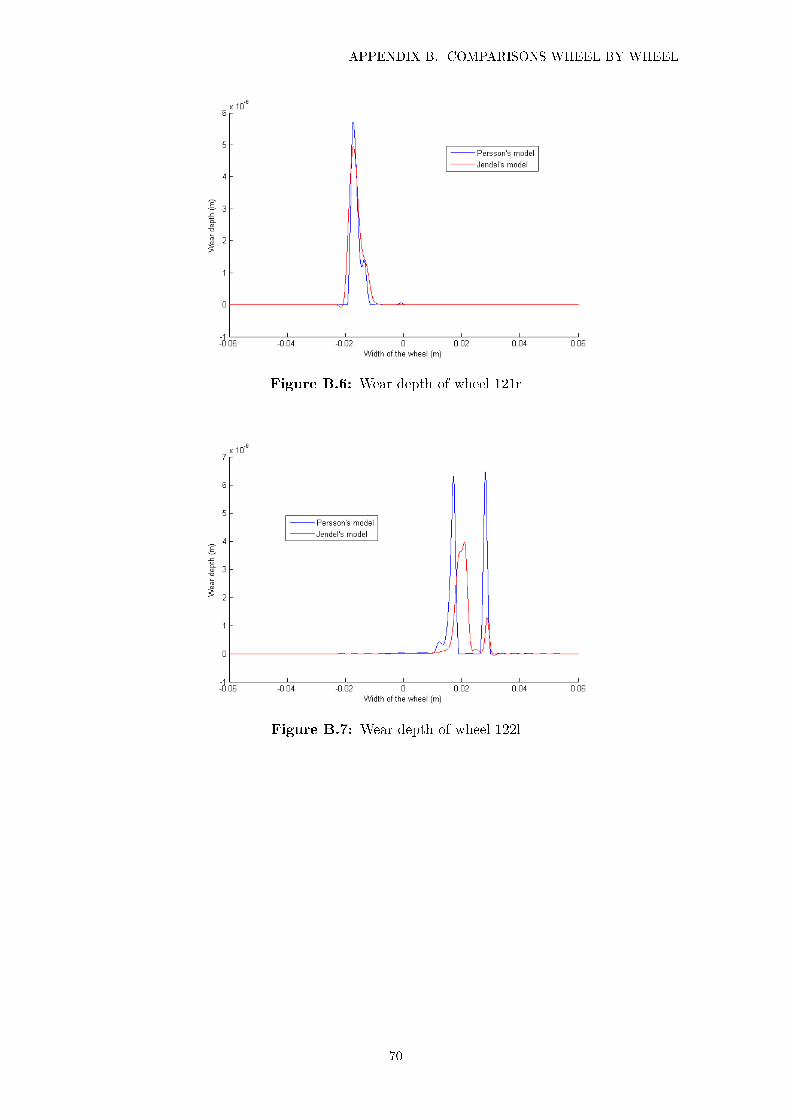
APPENDIX B. COMPARISONS WHEEL BY WHEEL
Figure B.6: Wear depth of wheel 121r
Figure B.7: Wear depth of wheel 122l
70
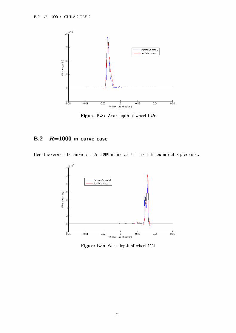
B.2. R=1000 M CURVE CASE
Figure B.8: Wear depth of wheel 122r
B.2 R=1000 m curve case
Here the case of the curve with R=1000 m and ht=0.1 m on the outer rail is presented.
Figure B.9: Wear depth of wheel 111l
71
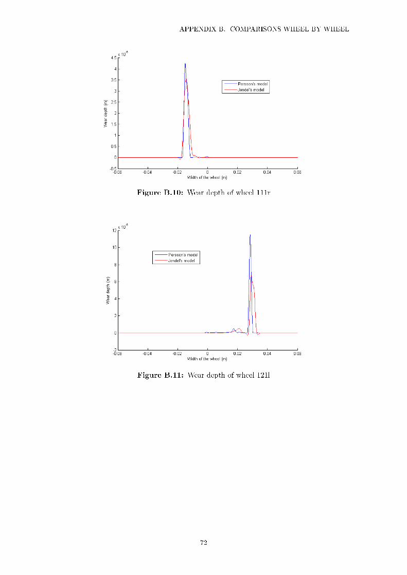
APPENDIX B. COMPARISONS WHEEL BY WHEEL
Figure B.10: Wear depth of wheel 111r
Figure B.11: Wear depth of wheel 121l
72

B.2. R=1000 M CURVE CASE
Figure B.12: Wear depth of wheel 121r
Figure B.13: Wear depth of wheel 112l
73

APPENDIX B. COMPARISONS WHEEL BY WHEEL
Figure B.14: Wear depth of wheel 112r
Figure B.15: Wear depth of wheel 122l
74

B.2. R=1000 M CURVE CASE
Figure B.16: Wear depth of wheel 122r
75

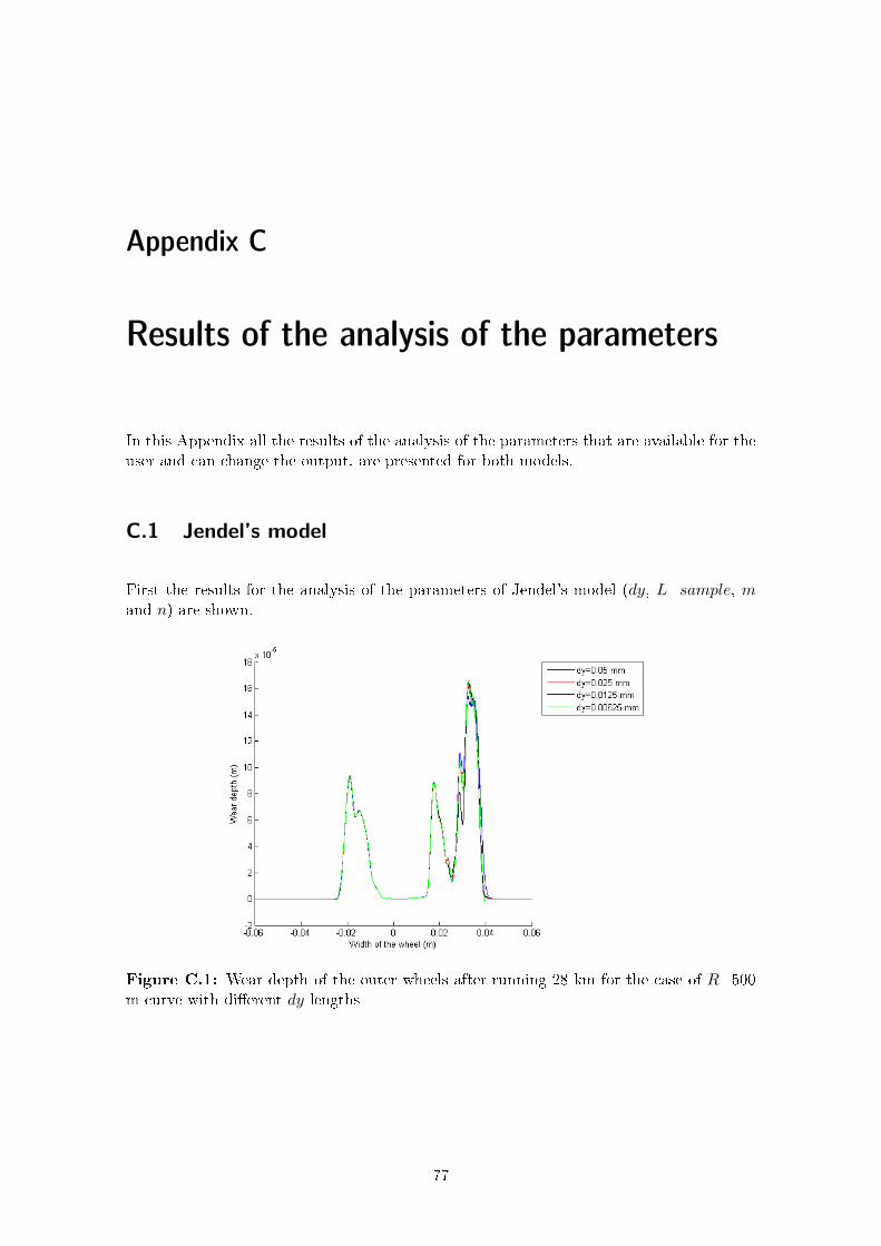
Appendix C
Results of the analysis of the parameters
In this Appendix all the results of the analysis of the parameters that are available for theuser and can change the output, are presented for both models.
C.1 Jendel’s model
First the results for the analysis of the parameters of Jendel's model (dy, L_sample, mand n) are shown.
Figure C.1: Wear depth of the outer wheels after running 28 km for the case of R=500m curve with di�erent dy lengths
77
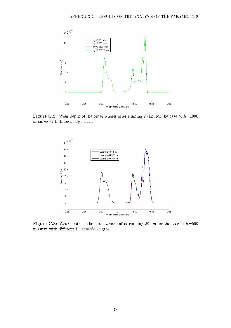
APPENDIX C. RESULTS OF THE ANALYSIS OF THE PARAMETERS
Figure C.2: Wear depth of the outer wheels after running 28 km for the case of R=1000m curve with di�erent dy lengths
Figure C.3: Wear depth of the outer wheels after running 28 km for the case of R=500m curve with di�erent L_sample lengths
78

C.1. JENDEL'S MODEL
Figure C.4: Wear depth of the outer wheels after running 28 km for the case of R=1000m curve with di�erent L_sample lengths
Figure C.5: Wear depth of the outer wheels after running 28 km for the case of R=500m curve with di�erent m and n parameters
79

APPENDIX C. RESULTS OF THE ANALYSIS OF THE PARAMETERS
Figure C.6: Wear depth of the outer wheels after running 28 km for the case of R=1000m curve with di�erent m and n parameters
C.2 Persson’s model
Now the results of the simulations for the parameters of Persson's model (Nintx, Ninty,m and n) are presented.
Figure C.7: Wear depth of the outer wheels after running 5.6 km for the case of R=500m curve with di�erent Nintx values
80

C.2. PERSSON'S MODEL
Figure C.8: Wear depth of the outer wheels after running 5.6 km for the case of R=1000m curve with di�erent Nintx values
Figure C.9: Wear depth of the outer wheels after running 5.6 km for the case of R=500m curve with di�erent Ninty values
81

APPENDIX C. RESULTS OF THE ANALYSIS OF THE PARAMETERS
Figure C.10: Wear depth of the outer wheels after running 5.6 km for the case of R=1000m curve with di�erent Ninty values
Figure C.11: Wear depth of the outer wheels after running 28 km for the case of R=500m curve with di�erent m and n parameters
82

C.2. PERSSON'S MODEL
Figure C.12: Wear depth of the outer wheels after running 28 km for the case of R=1000m curve with di�erent m and n parameters
83


