AMS 394 ANOVA using R 1 #One-way ANOVA #We are often interested in determining whether the means from more than two populations or groups are equal or not. To test whether the difference in means is statistically significant, we can perform analysis of variance (ANOVA) using the R function aov(). If the ANOV AF-test shows there is a significant difference in means between the groups we may want to perform multiple comparisons between all pair -wise means to determine how they differ. #A. Analysis of Variance #The first step in our analysis is to graphically compare the means of the variable of interest across groups. It is possible to create side-by-side boxplots of measurements organized in groups using the function plot(). Simply type plot(response ~ factor, data=data_name) where response is the name of the response variable and factor the variable that separates the data into groups. Both variables should be contained in a data frame called data_name. #Ex. A drug company tested three formulations of a pain relief medic ine for migraine headache sufferers. For the experiment 27 volunteer s were selected and 9 were randomly assigned to one of three drug formulations. The subjects were instructed to take the drug during t heir next migraine headache episode and to report their pain on a sc ale of 1 to 10 (10 being most pain). #Data: #Drug A 4 5 4 3 2 4 3 4 4 #Drug B 6 8 4 5 4 6 5 8 6 #Drug C 6 7 6 6 7 5 6 5 5 #To make side-by-side boxplots of the variable pain grouped by the variable drug we must first read in the data into the appropriate format. pain = c(4, 5, 4, 3, 2, 4, 3, 4, 4, 6, 8, 4, 5, 4, 6, 5, 8, 6, 6, 7, 6, 6, 7, 5, 6, 5, 5) drug = c(rep("A",9), rep("B",9), rep("C",9)) migraine = data.frame(pain,drug);migraine ## pain drug ## 1 4 A
Transcript
AMS 394 ANOVA using R
1
#One-way ANOVA
#We are often interested in determining whether the means from more
than two populations or groups are equal or not. To test whether the
difference in means is statistically significant, we can perform
analysis of variance (ANOVA) using the R function aov(). If the ANOV
AF-test shows there is a significant difference in means between the
groups we may want to perform multiple comparisons between all pair
-wise means to determine how they differ.
#A. Analysis of Variance
#The first step in our analysis is to graphically compare the means
of the variable of interest across groups. It is possible to create
side-by-side boxplots of measurements organized in groups using the
function plot(). Simply type plot(response ~ factor, data=data_name)
where response is the name of the response variable and factor the
variable that separates the data into groups. Both variables should
be contained in a data frame called data_name.
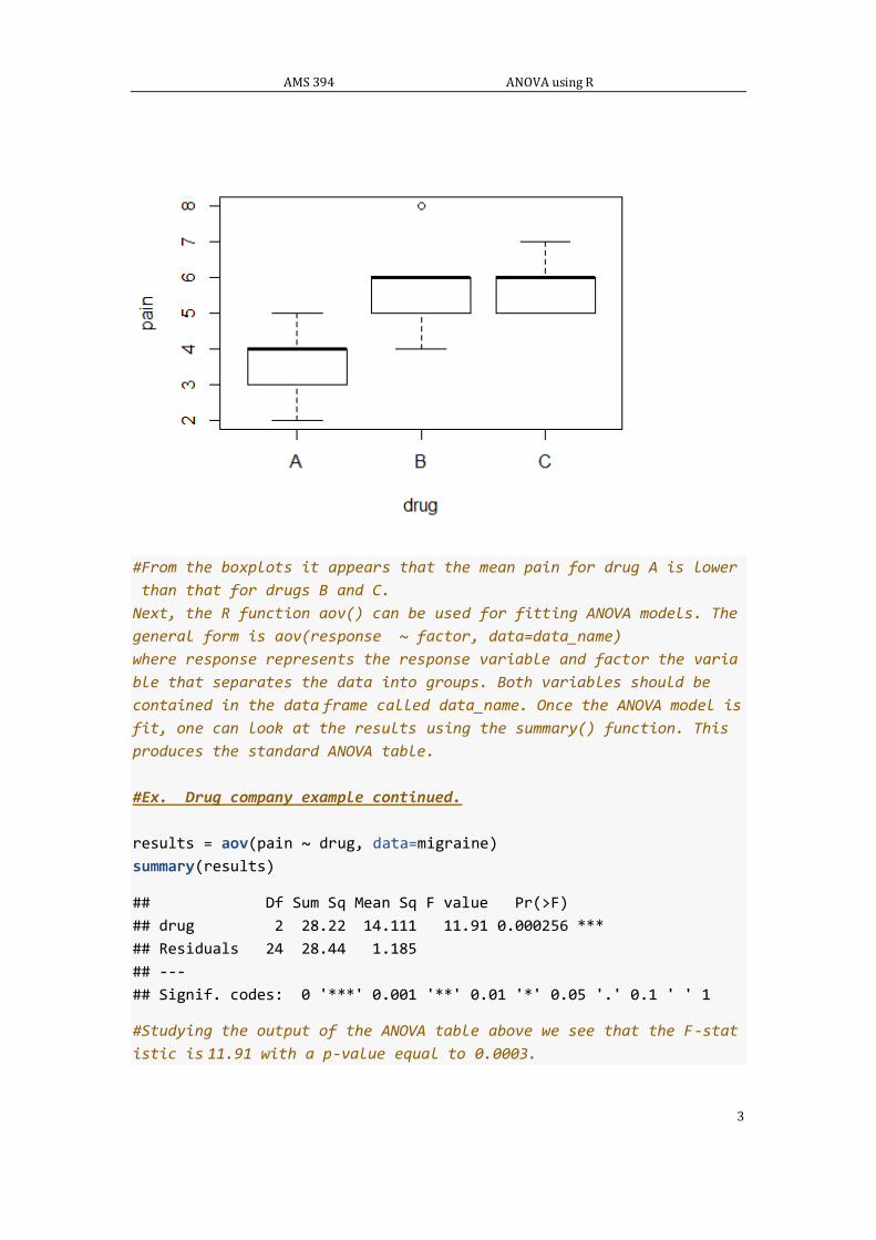
#Ex. A drug company tested three formulations of a pain relief medic
ine for migraine headache sufferers. For the experiment 27 volunteer
s were selected and 9 were randomly assigned to one of three drug
formulations. The subjects were instructed to take the drug during t
heir next migraine headache episode and to report their pain on a sc
ale of 1 to 10 (10 being most pain).
#Data:
#Drug A 4 5 4 3 2 4 3 4 4
#Drug B 6 8 4 5 4 6 5 8 6
#Drug C 6 7 6 6 7 5 6 5 5
#To make side-by-side boxplots of the variable pain grouped by the
variable drug we must first read in the data into the appropriate