A method of using functional magnetic resonance imaging (fMRI) tomeasure retinotopic organization within human cortex is described.The method is based on a visual stimulus that creates a travelingwave of neural activity within retinotopically organized visual areas.We measured the fMRI signal caused by this stimulus in visualcortex and represented the results on images of the flattenedcortical sheet. We used the method to locate visual areas and toevaluate the spatial precision of fMRI. Specifically, we: (i) identifiedthe borders between several retinotopically organized visual areas inthe posterior occipital lobe; (ii) measured the function relatingcortical position to visual field eccentricity within area V1; (iii)localized activity to within 1.1 mm of visual cortex; and (iv)estimated the spatial resolution of the fMRI signal and found thatsignal amplitude falls to 60% at a spatial frequency of 1 cycle per 9mm of visual cortex. This spatial resolution is consistent with alinespread whose full width at half maximum spreads across 3.5 mmof visual cortex.

In a series of experiments, we measured the retinotopic

organization of human cortical area V1 and identified the

locations of other nearby retinotopically organized visual areas.

We also used the retinotopic organization of human primary

visual cortex to measure the spatial localization and spatial

resolution that can be obtained from functional magnetic

resonance imaging (fMRI) of human visual cortex.

Human primary visual cortex (area V1) is located in the

occipital lobe within and surrounding the calcarine sulcus. Data

from human lesion studies showed that neurons within area V1

are retinotopically organized, following a roughly polar

coordinate system (Holmes, 1918, 1944; Horton and Hoyt,

1991a). As one moves from posterior to anterior in cortex, the

representation of the visual field shifts from the center to

the periphery. We will refer to this dimension of retinotopy as

eccentricity. As one moves from the lower to the upper lip of the

calcarine, the representation of the visual field shifts from

the upper vertical meridian through the horizontal meridian to

the lower vertical meridian. We will refer to this dimension of

retinotopy as polar angle. The locations of several visual field

landmarks are shown in Figure 1A, and the key features of the

cortical anatomy are shown in Figure 1B.

Because of the retinotopic organization of visual areas, it is

possible to create simple visual stimuli that generate continuous

traveling waves of neural activity in visual cortex. The stimulus

used to create the traveling wave and our initial measurements of

the wave were described brief ly in prior reports (Engel et al.,

1993, 1994). The travelling wave allows retinotopic organization

to be measured more efficiently and with higher spatial

precision than was possible in previous work that used static

stimuli (Fox et al., 1987; Schneider et al., 1993; Shipp et al.,

1995; Tootell, et al., 1995). As a result, our method has been

used widely to measure retinotopic organization in V1 and

adjacent cortical areas (DeYoe et al., 1994, 1996; Sereno et al.,

1995, Worden et al., 1995).

Here we present a new set of results using the traveling wave.

First, from measurements of the motion of the traveling wave,

we identified the borders between several retinotopically

organized visual areas in the posterior occipital lobe. Second, we

measured the function relating cortical position to visual field

eccentricity within area V1. Third, from measurements of the

reliability of the traveling wave we found that it is possible to

localize activity to within 1.1 mm of visual cortex. Fourth, from

measurements of the amplitude of the traveling wave using

stimuli with various spatial frequencies, we estimated the spatial

resolution of the fMRI signal. We found that signal amplitude

falls to 60% of maximum at a spatial frequency of 1 cycle per 9

mm of visual cortex. This spatial resolution is consistent with a

linespread whose full width at half maximum spreads across 3.5

mm of visual cortex.

Materials and Methods

Stimuli

Area V1 of human visual cortex responds well to patterned, f lickering

stimuli. Hence, to create a strong neural response within area V1 we used

a contrast-reversing checkerboard. The mean luminance of the f lickering

checkerboard field was 92 cd/m2; its contrast was close to 100%; its

contrast reversal rate was 8 Hz. The checkerboard pattern was

superimposed on a uniform field whose intensity was equal to the mean

intensity of the checkerboard. The stimuli were projected onto a

rear-projection viewing screen mounted within the scanner. Subjects

were supine and viewed the display by means of a mirror placed above

their eyes and housed in a custom-designed headpiece. Subjects’ head

positions were stabilized using a bite bar, and subjects were instructed to

fixate the center of the display throughout the stimulus presentation

period.

To create a traveling wave of neural activity within area V1, we

changed the position of the checkerboard pattern slowly over time.

Figure 2A shows an example of a stimulus designed to create a wave of

activity traveling from posterior to anterior calcarine. The f lickering rings

moved slowly across the visual field. In our experiments we used both

expanding ring and contracting ring stimuli. When an expanding ring

stimulus reached the edge of the viewing aperture (12° radius), it was

replaced by a new ring in the center of the display. When a contracting

ring stimulus reached the center, it was replaced by a new ring at the edge

of the stimulus aperture. In these experiments four cycles of this stimulus

were presented at a rate of one cycle either every 32 or 48 s.

Figure 2B shows that as the ring moves, the stimulus at each point in

the visual field alternates at 1/32 Hz; the stimulus at a location is a

f lickering contrast pattern half of the time and is the uniform gray

background the other half of the time. This alternation is delayed for

peripheral visual field locations compared with central ones.

The moving ring stimulus is designed to measure retinotopic

organization with respect to visual eccentricity. The f lickering

checkerboard gives rise to sustained neural activity at each location that

Retinotopic Organization in Human VisualCortex and the Spatial Precision ofFunctional MRI

Stephen A. Engel, Gary H. Glover and Brian A. Wandell

Department of Psychology, Neuroscience Program and

Department of Diagnostic Radiology, Stanford University,

Stanford, CA 94305, USA

Cerebral Cortex Mar 1997;7:181–192; 1047–3211/97/$4.00

modulates at the stimulus alternation frequency (1/32 Hz). As the stimulus

moves from fovea to periphery the activity at locations containing

neurons with peripheral receptive fields is delayed relative to locations

containing neurons with foveal receptive fields, creating a traveling wave

of neural activity. Because the neural activity alternates periodically, the

delay can be measured by the phase of the neural activity.

To measure retinotopic organization with respect to polar angle, we

used rotating patterns with three wedges, such as the one shown in

Figure 2C, or a similar pattern with a single wedge. Subjects fixated at the

center of the visual field while the wedges of contrast-reversing f licker,

presented on a uniform gray field, rotated about the fixation point. The

contrast reversal rate and the stimulus cycle time for the f lickering

wedges were the same as for the moving ring stimulus.

The rotating wedge stimulus is designed to measure retinotopic

organization with respect to polar angle. As the stimulus rotates, activity

at V1 locations containing neurons whose receptive fields are further

along the direction of rotation will be delayed relative to locations

containing neurons whose receptive fields are near the stimulus starting

position. This stimulus creates a traveling wave of activity moving

between the representations of the upper and lower vertical meridia.

Again, because the neural activity alternates periodically, the delay can be

measured by the phase of the neural activity.

Measurement Planes

Planes were selected in one of three orientations. To track activity

traveling from posterior to anterior calcarine we acquired data in either a

sagittal slice or an oblique plane parallel to the calcarine sulcus. To track

activity traveling from the superior to the inferior lips of the calcarine we

measured in a plane perpendicular to the calcarine sulcus.

Magnetic Resonance Protocols

Functional MR images were acquired continuously as subjects viewed the

projected stimulus. Measurements were made with a GE Signa 1.5T

scanner using a spiral k-space acquisition (Meyer et al., 1992). We

measured gradient-echo BOLD (T2*) contrast (Kwong et al., 1992; Ogawa

et al., 1992).

In our initial experiments data were acquired in a single measurement

plane using a typical TE of 40 ms, TR of 75 ms and f lip angle of 23°.

During each 192 s experiment, 128 images per plane were acquired (1.5

s/image) with an in-plane resolution of 1.03 mm and a through-plane

resolution of 5 mm. The data were interpolated onto a 256 × 256 grid,

yielding an in-plane pixel size of 0.78 mm.

In later experiments four or eight planes of data were acquired in each

experiment; a typical TE was 40 ms, TR was 300 or 750 ms and f lip angle

was 35°. These experiments were of coarser spatial resolution: in-plane

resolution was roughly 1.6 mm; through plane resolution was generally

Figure 1. Visual field landmarks and their cortical representations are shown. (A) A representation of the visual field showing the fixation point (F), horizontal meridian (HM) and theupper and lower vertical meridia (UVM and LVM). The polar angle increases in the clockwise direction around the circle, and eccentricity increases from the fixation point to theperipheral visual field. (B) A medial view of human occipital lobe is shown. PO, Parieto-occipital sulcus; CC, corpus callosum; C, calcarine sulcus. The representations of the upper andlower vertical meridia are indicated by the dashed lines; these meridia define the borders between area V1 and the surrounding visual area, V2. An additional representation of thehorizontal meridian runs along the deepest part of the calcarine sulcus and is not visible from this view point. Other representations of the horizontal meridian define the borders ofdorsal V2 with area V3 and of ventral V2 with area VP. This figure was adapted from Horton and Hoyt (1991b).

Figure 2. Stimuli used to create traveling waves of neural activity in retinotopicallyorganized cortex are shown. The stimuli were composed of a contrast-reversingcheckerboard pattern flickering at 8 Hz. (A) The expanding ring stimulus is shown at fivemoments in time spanning one stimulus cycle. (B) At each location within the visualfield, the stimulus follows a square-wave alternation between the contrast-reversingrings and the uniform gray field. The expanding ring stimulus was delayed in theperiphery relative to the center; hence, the temporal phase of the square-wavealternation varied as a function of distance from the center of the visual field. Twostimulus cycles are shown. (C) The rotating wedge stimulus is shown at five momentsin time spanning one stimulus cycle.

182 fMRI of Visual Cortex • Engel et al.

4.0 mm. One image from each measurement plane was acquired every

2 s. In all experiments T1-weighted in-plane anatomical scans were taken

in the functional measurement planes in order to register the functional

and anatomical data. These anatomical images had an in-plane spatial

resolution of 0.78 × 0.78 mm and a through-plane resolution of 5 mm.

Data Analysis

Time Series Analysis

The fMRI protocol yielded a time series of data at each pixel. We used two

quantities to characterize each pixel’s responses. First, we used the phase

of the harmonic function (harmonic functions here refer to the set of

functions comprising sinusoids at any phase and frequency) at the

stimulus frequency that best correlated with the time series data

(Bandettini et al., 1993). This response phase measures the relative delay

of stimulus driven activity at each pixel. We used the signal delay to infer

the location of the receptive fields of the neurons whose activity gave rise

to that pixel’s time series data. We calculated the response phase using

the discrete Fourier transform of the time series (see Appendix).

Second, we measured response magnitude as the correlation

between the pixel time series and the best-correlated harmonic at the

stimulus alternation frequency. We used the response magnitude to create

the activity maps (Fig. 5) and to perform the spatial resolution analysis

(Fig. 11). The correlation coefficient is the amplitude of the response at

the stimulus frequency divided by the square root of the time series

power; this quantity was calculated using the discrete Fourier transform

of the time series (see Appendix).

For most of the stimuli we used, the harmonic frequency that best

correlated with the response was equal to the stimulus frequency. As we

describe below, this need not be the case; for some types of stimuli a

significant response occurred at other frequencies (see Fig. 6). For the

other experiments we describe, the principal response was at the

stimulus frequency.

In the analyses reported below, we selected pixels in one of two ways.

Some analyses were performed along linear regions of interest that were

selected by hand from in-plane anatomical images. Others were

performed on all pixels that were identified as containing gray matter;

these were selected as the first step in the cortical f lattening method

described below.

Images of Flattened Cortex

In order to visualize data from many measurement planes, we created a

single f lattened representation of cortex. We performed this analysis

using a procedure described more fully elsewhere (Wandell et al., 1996).

The method is similar to other computational methods that have been

developed for f lattening cortex (Schwartz, 1990; Dale and Sereno, 1993;

Carman et al., 1995; Drury et al., 1996).

Brief ly, we created f lattened representations in four steps. First, we

acquired a volume of anatomical images that spanned the part of cortex

to be f lattened. Second, a connected volume of gray matter was identified

in the anatomical data, using a graphical software tool. Third, a fully

automated algorithm assigned image positions to the sampled set of the

identified gray matter pixels. The planar representation of the samples

was computed using an iterative algorithm based on metric multi-

dimensional scaling. Fourth, the planar positions of the remaining gray

matter points were assigned by interpolation. (The software used to

create these images has been archived and can be obtained from

http://white.stanford.edu)

To view the fMRI measurements on the f lattened representation, the

user identified corresponding locations in the in-plane anatomies and the

anatomical volume. The fMRI measurements were aligned with the

anatomical volume by finding the best (least-squares) translation and

rotation between the set of corresponding anatomical locations (Arun et

al., 1987). From this alignment, each gray matter location that falls in the

functional planes was assigned a functional measurement. We generated

images of activity by displaying each gray matter point’s functional

measurement at its location in the f lattened representation. In images of

functional activity on the f lattened cortical representation, only gray

matter points that fell within the functional scan planes are shown.

After the gray matter locations were placed within the f lattened

image, they did not fill the image plane continuously. To generate a

continuous representation of the data, we interpolated: each image pixel

in the f lattened representation was assigned a weighted average of the

neighboring pixels that contained data. The weights assigned to each

neighbor were a Gaussian function of the distance to that neighbor.

Figure 3A is a view of the medial surface of an occipital lobe. Figure 3B

is a f lattened representation of this portion of cortex; the f lattened

representation was created using the algorithm described above. The

position of each point in Figure 3B shows the location of a gray matter

point in the f lattened cortical manifold. The brightness of each point

represents its relative position along the medial–lateral axis in the brain.

Light points represent gray matter near the medial plane and dark points

represent gray matter closer to the lateral aspect of the brain. The

calcarine sulcus is easy to identify on the f lattened representation

Figure 3. Two representations of the cortical sheet in the medial occipital lobe areshown. (A) A view of the medial surface of an occipital lobe is shown. ACS, anteriorcalcarine sulcus; ULC, upper lip of the calcarine; LLC, lower lip of the calcarine. The starrepresents a location near the occipital pole. (B) The same cortical region is shown in aflattened representation that was created by the method described in the text. Thebrightness of each image point represents the relative position along the medial–lateralaxis in the brain. The dashed line traces the deepest part of the calcarine sulcus, andthe star again indicates the location of the occipital pole. In this and all subsequentfigures, scale bars indicate 1 cm.

Cerebral Cortex Mar 1997, V 7 N 2 183

because its fundus, which is closer to the lateral aspect of the brain,

appears as a dark band, and its lips appear as light regions surrounding

the sulcus. [In subsequent figures we use color or brightness to represent

functional data. On these f lattened representations, we will continue to

indicate the positions of the deepest part of the calcarine sulcus (dashed

line) and the occipital pole (star).]

We evaluated how accurately the algorithm preserved distances

between gray matter points by comparing, for each pair of points, the

separation in the cortical manifold and in the f lattened representation.

For the points shown in the figure, spanning over a 100 cm2 region of gray

matter, distances between pairs of points in the image of f lattened cortex

differed from the true cortical manifold distances with a roughly Gaussian

distribution with an SD of 3 mm.

Results

Basic Measurements

The first set of experiments showed that the moving ring

stimulus created a traveling wave of activity that could be

observed in the fMRI signal. We used a contracting ring stimulus,

measured the fMRI signal in a plane parallel to the calcarine

sulcus and analyzed data along the linear region of interest

within area V1 indicated in black in Figure 4C. We expected the

stimulus to create a traveling wave of activity moving from

anterior to posterior along the region of interest.

Figure 4A shows the time varying fMRI signal at points along

the region of interest. The fMRI signal is a traveling wave that

moves from anterior to posterior portions of cortex. Figure 4B

shows the delay in activity at points along the region of interest,

as measured by the response phase. This plot shows that, as

expected, the fMRI signal was delayed at posterior portions of

the calcarine relative to the signal at more anterior locations.

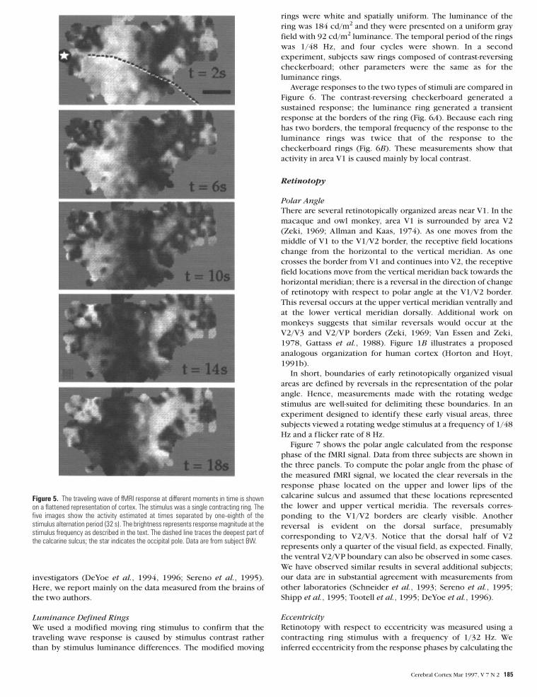
Figure 5 shows the results of a similar traveling wave

experiment displayed on a f lattened image of cortex. In these

five images the gray level values ref lect the spatial pattern of the

fMRI response magnitude at different moments in time during

the stimulus cycle. The fMRI signal shown in Figure 5 was

generated during an experiment in which the stimulus consisted

of contracting ring stimuli with one ring. The stimulus

alternation frequency was 1/32 Hz. In Figure 5 each pixel’s gray

level represents the response magnitude multiplied by a unit

harmonic at the response phase. These images represent that

portion of the fMRI signal at the stimulus frequency. The bright

band of fMRI signal in the images shifts along the cortex. (A

more finely sampled sequence of these images as a movie can be

seen at http://white.stanford.edu/wandell)

We have measured this traveling wave in many experiments

on 12 subjects. While the signal-to-noise varied among subjects,

most locations where the scan plane intersected the posterior

calcarine sulcus yielded a signal that easily stood out from noise.

The traveling wave has also been measured by other

Figure 4. The traveling wave observed in area V1. (A) The time course of the fMRI signal at each of the locations within the region of interest during a single experiment is shown.The stimulus consisted of a single, contracting contrast-reversing ring, the stimulus period was 32 s and the stimulus was repeated six times. The horizontal axes show time andposition along the region of interest. The vertical axis shows the deviation of the fMRI signal from the mean level. The plotted waveform is a smoothed version of the data, computedby convolving the fMRI data with a Gaussian kernel (σx = 3 mm, σt = 6 s) and subsampling the result. (B) The phase in radians of the best-correlated harmonic at the stimulusalternation frequency (1/32 Hz) is shown as a function of position along the region of interest. (C) An anatomical image in the plane of the calcarine is shown. The black line showsthe gray matter along the calcarine that was used for the region of interest. The data are from subject BW.

184 fMRI of Visual Cortex • Engel et al.

investigators (DeYoe et al., 1994, 1996; Sereno et al., 1995).

Here, we report mainly on the data measured from the brains of

the two authors.

Luminance Defined Rings

We used a modified moving ring stimulus to confirm that the

traveling wave response is caused by stimulus contrast rather

than by stimulus luminance differences. The modified moving

rings were white and spatially uniform. The luminance of the

ring was 184 cd/m2 and they were presented on a uniform gray

field with 92 cd/m2 luminance. The temporal period of the rings

was 1/48 Hz, and four cycles were shown. In a second

experiment, subjects saw rings composed of contrast-reversing

checkerboard; other parameters were the same as for the

luminance rings.

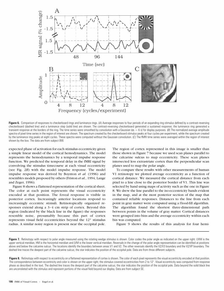
Average responses to the two types of stimuli are compared in

Figure 6. The contrast-reversing checkerboard generated a

sustained response; the luminance ring generated a transient

response at the borders of the ring (Fig. 6A). Because each ring

has two borders, the temporal frequency of the response to the

luminance rings was twice that of the response to the

checkerboard rings (Fig. 6B). These measurements show that

activity in area V1 is caused mainly by local contrast.

Retinotopy

Polar Angle

There are several retinotopically organized areas near V1. In the

macaque and owl monkey, area V1 is surrounded by area V2

(Zeki, 1969; Allman and Kaas, 1974). As one moves from the

middle of V1 to the V1/V2 border, the receptive field locations

change from the horizontal to the vertical meridian. As one

crosses the border from V1 and continues into V2, the receptive

field locations move from the vertical meridian back towards the

horizontal meridian; there is a reversal in the direction of change

of retinotopy with respect to polar angle at the V1/V2 border.

This reversal occurs at the upper vertical meridian ventrally and

at the lower vertical meridian dorsally. Additional work on

monkeys suggests that similar reversals would occur at the

V2/V3 and V2/VP borders (Zeki, 1969; Van Essen and Zeki,

1978, Gattass et al., 1988). Figure 1B illustrates a proposed

analogous organization for human cortex (Horton and Hoyt,

1991b).

In short, boundaries of early retinotopically organized visual

areas are defined by reversals in the representation of the polar

angle. Hence, measurements made with the rotating wedge

stimulus are well-suited for delimiting these boundaries. In an

experiment designed to identify these early visual areas, three

subjects viewed a rotating wedge stimulus at a frequency of 1/48

Hz and a f licker rate of 8 Hz.

Figure 7 shows the polar angle calculated from the response

phase of the fMRI signal. Data from three subjects are shown in

the three panels. To compute the polar angle from the phase of

the measured fMRI signal, we located the clear reversals in the

response phase located on the upper and lower lips of the

calcarine sulcus and assumed that these locations represented

the lower and upper vertical meridia. The reversals corres-

ponding to the V1/V2 borders are clearly visible. Another

reversal is evident on the dorsal surface, presumably

corresponding to V2/V3. Notice that the dorsal half of V2

represents only a quarter of the visual field, as expected. Finally,

the ventral V2/VP boundary can also be observed in some cases.

We have observed similar results in several additional subjects;

our data are in substantial agreement with measurements from

other laboratories (Schneider et al., 1993; Sereno et al., 1995;

Shipp et al., 1995; Tootell et al., 1995; DeYoe et al., 1996).

Eccentricity

Retinotopy with respect to eccentricity was measured using a

contracting ring stimulus with a frequency of 1/32 Hz. We

inferred eccentricity from the response phases by calculating the

Figure 5. The traveling wave of fMRI response at different moments in time is shownon a flattened representation of cortex. The stimulus was a single contracting ring. Thefive images show the activity estimated at times separated by one-eighth of thestimulus alternation period (32 s). The brightness represents response magnitude at thestimulus frequency as described in the text. The dashed line traces the deepest part ofthe calcarine sulcus; the star indicates the occipital pole. Data are from subject BW.

Cerebral Cortex Mar 1997, V 7 N 2 185

expected phase of activation for each stimulus eccentricity given

a simple linear model of the cortical hemodynamics. The model

represents the hemodynamics by a temporal impulse response

function. We predicted the temporal delay in the fMRI signal by

convolving the stimulus timecourse at each visual eccentricity

(see Fig. 2B) with the model impulse response. The model

impulse response was derived by Boynton et al. (1996) and

resembles models proposed by others (Friston et al., 1994; Lange

and Zeger, 1996).

Figure 8 shows a f lattened representation of the cortical sheet.

The color at each point represents the visual eccentricity

encoded at that position. The foveal response is visible in

posterior cortex. Increasingly anterior locations respond to

increasingly eccentric stimuli. Retinotopically organized re-

sponses extend along a 3–4 cm strip of cortex. Beyond this

region (indicated by the black line in the figure) the responses

resemble noise, presumably because this part of cortex

represents visual field eccentricities beyond the 12° stimulus

radius. A similar noisy region is present near the occipital pole.

The region of cortex represented in this image is smaller than

those shown in Figure 7 because we used scan planes parallel to

the calcarine sulcus to map eccentricity. These scan planes

intersected less extrastriate cortex than the perpendicular scan

planes used to map the polar angle.

To compare these results with other measurements of human

V1 retinotopy we plotted average eccentricity as a function of

cortical distance. We measured the cortical distance from each

pixel to a line close to the posterior border of V1. This line was

selected by hand using maps of activity such as the one in Figure

8. We drew the line parallel to the iso-eccentricity bands evident

in the map, and at the most posterior section of the map that

contained reliable responses. Distances to the line from each

point in gray matter were computed using a f lood-fill algorithm.

The algorithm found the shortest three-dimensional path

between points in the volume of gray matter. Cortical distances

were grouped into bins and the average eccentricity within each

bin was computed.

Figure 9 shows the results of this analysis for four hemi-

Figure 6. Comparison of responses to checkerboard rings and luminance rings. (A) Average responses to four periods of an expanding ring stimulus defined by a contrast-reversingcheckerboard (dashed line) and a luminance step (solid line) are shown. The contrast-reversing checkerboard generated a sustained response; the luminance ring generated atransient response at the borders of the ring. The time series were smoothed by convolution with a Gaussian (σt = 6 s) for display purposes. (B) The normalized average amplitudespectra of pixel time series in the region of interest are shown. The spectrum created by the checkerboard stimulus peaks at four cycles per experiment, while the spectrum createdby the luminance ring peaks at eight cycles. These spectra were computed without the Gaussian convolution. (C) The fMRI time series were averaged within the region of interestshown by the box. The data are from subject BW.

Figure 7. Retinotopy with respect to polar angle measured using the rotating wedge stimulus is shown. Color codes the polar angle as indicated on the upper right: UVM is theupper vertical meridian, HM is the horizontal meridian and LVM is the lower vertical meridian. Reversals in the change of the polar angle representation can be identified at positionsabove and below the calcarine sulcus. The locations identify the boundary between areas V1 and V2. The other reversals identify the V2/V3 boundary and the V2/VP boundary. Thedashed line traces the deepest part of the calcarine sulcus; the star indicates the position of the occipital pole. Data are from three different subjects.

Figure 8. Retinotopy with respect to eccentricity on a flattened representation of cortex is shown. The color of each pixel represents the visual eccentricity encoded at that position.The correspondence between eccentricity and color is shown on the upper right; the stimulus covered eccentricities from 2 to 12°. Visual eccentricity was computed from responsephase as described in the text. The dashed line traces the deepest part of the calcarine sulcus; the star indicates the position of the occipital pole. Data beyond the solid black lineare uncorrelated with the stimulus and represent portions of the visual field beyond our display. Data are from subject SE.

186 fMRI of Visual Cortex • Engel et al.

Cerebral Cortex Mar 1997, V 7 N 2 187

spheres. The line that was used to measure cortical distance fell

at positions that represented slightly different eccentricities in

the different hemispheres. To compare data across hemispheres,

we aligned the four data sets at the point representing 10° of

eccentricity. The smooth curve is the exponential function

exp(0.063(d + 36.54)) that best fit (least-squares) the data, where

d is the cortical distance in mm.

Spatial Localization

Next, we measured how accurately the response to the moving

ring stimulus can be localized. The measurements were based on

the following logic. Consider the response to a single frame of

the moving ring stimulus. The cortical locations responding to

that frame are those locations whose fMRI signal has a particular

response phase. Cortical locations responding to the next frame

in the stimulus will have a slightly different response phase.

Thus, the response to a particular stimulus frame will be well

localized when the cortical locations with its response phase can

be reliably discriminated from the cortical locations at the

response phase of the next frame. Factors such as noise in the

fMRI signal and spatial and temporal sampling limit our ability to

localize the response phase.

To measure how accurately the response phases can be

localized, we made measurements in a plane within the calcarine

sulcus. The measurement plane intersected linear regions in

both the right and the left calcarine sulci. The stimulus

contained two contrast-reversing rings. In one experiment the

rings traveled outward (expanding) and in a second experiment

they traveled toward the fixation mark (contracting). The

stimulus period was 48 s and the experiment lasted for four

periods.

In order to calculate the localization precision we estimated

the response phase separately for each stimulus cycle and each

pixel. These estimates were used to compute a mean and

standard error of the phase for each pixel. Figure 10 shows the

mean and standard errors of the phase estimated within two

regions of interest for the two stimuli.

The modal standard error of the phase estimate across pixels

in both regions of interest was 0.33 radians. The modal values

were similar in the right and left calcarine, and for expanding

and contracting rings. The modal rate of change of the temporal

phase along the two regions of interest (i.e. the slopes of the

lines in Figure 10) was ∼0.60 radians/mm. Hence, a reliable (two

standard errors of the mean) phase separation corresponds to

0.66 rad/0.60 (rad/mm) 1.1 mm, which is close to our previous

estimate of 1.3 mm (Engel et al., 1994).

We interpret this value as an upper bound on the precision of

the localization under these conditions. Of course, differences in

stimuli, brain regions and signal-to-noise ratios will inf luence the

spatial localization obtainable in other conditions.

Spatial Resolution

We evaluated the spatial resolution of the fMRI signal by

estimating the modulation transfer function (MTF). In general,

the MTF describes how the signal varies with increasing spatial

frequency. We used the MTF to analyze how well the fMRI signal

captures the spatial pattern of cortical activity.

To generate patterns of cortical activity at increasing spatial

frequency, we used stimuli with one, two, three and four moving

rings. The temporal frequency of the stimuli in all four

conditions moved was held constant at 1/48 Hz by adjusting the

velocity of the moving rings. The rings reversed their contrast at

8 Hz.

We expected each ring to generate a traveling wave of

activity. As the number of stimulus rings increased, the distance

between the traveling waves decreased and the falling edge of

one wave overlapped with the rising edge of its neighboring

wave. Increasing the stimulus spatial frequency caused more

overlap and reduced the temporal modulation of the fMRI signal

measured at each pixel. Thus, we evaluated spatial resolution by

measuring the fall off in the response magnitude as a function of

the cortical separation between the traveling waves. We

measured the separation between the waves in terms of their

cortical frequency, which has units of cycles per mm of cortex.

Cortical frequency at each location in gray matter was

calculated using measurements of retinotopy with respect to

eccentricity. As described earlier, these measurements can be

summarized by computing an exponential function that relates

eccentricity to cortical distance (see Fig. 9 and accompanying

text). We estimated the parameters of one such function for each

hemisphere using the data obtained in the one ring condition.

The derivative of this function specified the the number of

degrees of visual angle represented in 1 mm of cortex at each

gray matter location (deg/mm) for that hemisphere. Multiplying

the stimulus spatial frequency (cycles/deg) by this derivative

(deg/mm) yielded the cortical frequency (cycles/mm) for each

gray matter location.

We estimated the MTF by plotting response magnitudes from

all four stimulus conditions and gray matter locations as a

function of cortical frequency. Figure 11 shows such a plot for

one hemisphere. To make this plot, data were binned by cortical

frequency and the average of each bin is plotted. The smooth

curve is a scaled Gaussian (SD = 0.11 cycles/mm) fit to these

averages (least-squares) after subtracting out a baseline cor-

relation that represents correlation due to noise. (The baseline

correlation was estimated in two ways. We measured

correlations in peripheral regions of V1 that showed no coherent

Figure 9. Visual field eccentricity as a function of distance from the 10° point in V1 isshown for four hemispheres. Eccentricity was computed from response phase; corticaldistances were measured along the gray matter from a line close to the posteriorborder of V1. Cortical distances were grouped into bins and the average eccentricitywithin each bin was computed. Each symbol type represents data from one hemispherefrom either subject SE or BW. The data have been shifted to align at the 10° eccentricitypoint. The smooth curve is the exponential function exp(0.063(d + 36.54)) that best fit(least-squares) the data, where d is cortical distance (mm).

188 fMRI of Visual Cortex • Engel et al.

signal. We also examined correlations to harmonics that differed

from the stimulus frequency. The two estimates agreed well.)

We performed this experiment in two subjects (four

hemispheres) and the estimated SDs were 0.19, 0.11, 0.08, 0.07,

yielding a mean of 0.11. The Gaussian function falls to 60.65% of

its maximum at 1 SD from the mean. On average, then, the signal

amplitude falls to ∼60% of its maximum at 0.11 cycles/mm or

equivalently at 1 cycle in 9 mm of cortex.

Discussion

Visual Areas

One of the most important applications of the traveling wave

measurements is the segregation of retinotopically organized

visual areas in human cortex. Our method segregates these visual

areas clearly and reliably, and this observation has been

confirmed by other groups (e.g. Sereno et al., 1995; DeYoe et al.,

1996). We have measured both borders of a retinotopically

organized region surrounding V1, revealing a likely candidate for

human V2. Retinotopic organization continues beyond this

region to presumptive V2/V3 and V2/VP borders as well. Figure

7 shows three good examples of these borders. These results also

agree with measurements made using static stimuli (Schneider et

al., 1993; Shipp et al., 1995; Tootell et al., 1995).

V1 Retinotopy

Figure 12 shows our results along with other estimates of the

retinotopic organization of human primary visual cortex. The

solid black line is an exponential curve fit to the data shown in

Figure 9. The open symbols were computed from two linear

regions of interest in single plane expanding ring experiments

(Engel et al., 1994). The dashed line is an estimate based on

human stroke patients and electrophysiological data from

non-human primates (Horton and Hoyt, 1991a); the ‘x’s are from

Sereno et al. (1995), who used fMRI methods similar to the ones

described here. To compare the various results, we aligned the

data at the location of the representation of the 10° point. There

is substantial agreement among all these measurements as well as

those obtained using other methods (see figure 2 in Engel et al.,

1994).

There have been two different reports concerning the extent

of the representation of the central 2° in the human area V1.

Horton and Hoyt (1991a) report that the central 2° covers <20

mm of cortical distance; Sereno et al. (1995) suggest that the

central 2° extends over >30 mm of cortical distance. Because the

Figure 10. Standard errors of the response phase measurements were used toestimate localization precision. Response phases were estimated separately for eachstimulus cycle. The mean and standard error of the estimates at various positions alongthe calcarine sulcus are shown. Error bars represent 2 standard errors. The top panelsshow measurements using expanding rings and the bottom panels showmeasurements with contracting rings. Panels on the left show measurements from theleft calcarine and panels on the right from the right calcarine. The data are from subjectBW.

Figure 12. Comparison of retinotopic measurements of human V1. Retinal eccentricityas a function of cortical distance relative to the 10° point is shown. The open symbolsare measurements from two observers in Engel et al. (1994). The solid curve shows thebest fitting exponential (least-squares) to the four hemispheres measured in this study.The dotted line shows an estimate derived from scotoma in human stroke patients andelectrophysiological data from non-human primates (Horton and Hoyt, 1991a). The ‘x’sare fMRI measurements by Sereno et al. (1995).

Figure 11. Analysis of the spatial resolution of fMRI. Average fMRI responsemagnitude is shown as a function of cortical frequency. Cortical frequency wascalculated as described in the text. The error bars represent 2 standard errors. Thesmooth curve is the scaled Gaussian (SD = 0.11) that best fits (least-squares) the data.The Gaussian function falls to 60.65% of its maximum at 1 SD from the mean; so, theaverage correlation is at roughly sixty percent of its maximum at 0.11 cycles/mm, or 1cycle per 9 mm. These data are from subject BW.

Cerebral Cortex Mar 1997, V 7 N 2 189

fixation spot in our experiments occupied the central 0.5°, and

because of the presence of small eye movements, we could not

make measurements below 1°. However, in our data the

representation of the 2° point generally falls in a part of V1 found

near the posterior pole. Our measurements could be consistent

with those of Sereno et al. (1995) if area V1 extends at least 3 cm

around the posterior pole onto the lateral surface. While

anatomical investigations agree that V1 can extend onto the

lateral surface, none finds such a large extension (Stensaas et al.,

1974; Rademacher et al., 1993). Hence, our measurements are in

general agreement with those of Horton and Hoyt (1991a).

Localization and Resolution

Our measurements of the traveling wave show that the fMRI

signal can be localized to within 1.1 mm. This precision was

achieved in 192 s experiments using a 1.5T instrument. Our

measurements of response magnitude as a function of cortical

frequency of the traveling wave show that the modulation

transfer function falls off as a Gaussian function with an SD of

0.11 cycles/mm. Signals at higher cortical frequencies can be

measured; the upper limit on detectable cortical frequency

depends on the signal-to-noise ratio of the measurement.

To the extent that the relationship between neural activity

and the fMRI signal can be modeled accurately by a symmetric

shift-invariant linear system, the system’s linespread function

can be computed directly from its MTF (e.g. Bracewell, 1978).

Intuitively, the linespread function defines the cortical spread

measured when stimulating with a very fine f lickering line, and

when the MTF is a Gaussian function, the linespread is also

Gaussian. We have not tested whether the relationship between

neural activity and the fMRI signal is linear; should this test fail,

neither the linespread nor the MTF completely characterize the

spatial resolution of the fMRI signal. We computed that the

linespread function associated with our MTF measurements is a

Gaussian function with a full width at half maximum amplitude

of 3.5 mm. This value is close to the neural linespread estimated

in the macaque by optical imaging with voltage sensitive dye

(Grinvald et al., 1994).

There are several potential sources of the spatial spread in the

fMRI signal. A portion of the spread may be due to lateral neural

connections within the cortex; another portion may be due to

the response of the vasculature to focal neural activity; finally,

some part of the spreading must be due to experimental artifacts

such as slight head movements, brain pulsatility and optical

defocus. The agreement between the fMRI measurements and

the neural linespread estimated in the macaque (Grinvald et al.,

1994) suggests that lateral connections in V1 may be the limiting

factor in the spatial resolution of the fMRI signal.

For a number of reasons the localization and resolution

estimates obtained in these experiments may not provide a

general rule for the brain. First, the vascularization in area V1 is

relatively dense (Zheng et al., 1991). Both localization and

resolution precision may depend upon this vascularization.

Second, localization and resolution depend on the signal-to-noise

ratio, which depends on a number of factors, including the

stimulus, task, brain region, pulse sequence and MR device.

Third, for many parts of the brain we do not yet know how to

create stimuli or tasks that generate focal activity. Consequently,

it is not possible to generalize from the measurements reported

here to experiments in other brain regions. Nonetheless, our

results do show quite clearly that fMRI can yield fine spatial

precision in experiments lasting only a few minutes.

Source of the fMRI Signal

Because BOLD contrast arises from changes in blood

oxygenation, large veins produce measurable signal. Some

research suggests that most of the signal comes from

macroscopic vessels (Lai et al., 1993). This would present a

problem for some fMRI applications because large vessels pool

blood from relatively large regions of cortex and their

oxygenation level only informs us about the average activity over

these regions. Whether the BOLD contrast arises only from large

veins is controversial; some evidence suggests that a significant

portion of the signal arises from the cortical capillary bed

(Menon et al., 1995).

Our estimate of the MTF supports the view that a significant

portion of the fMRI signal arises from vessels serving fairly small

regions of cortex. Figure 11 shows that we observe significant

correlations at cortical frequencies at least as high as 1 cycle per

6 mm (0.1667 cycles/mm). Hence, vessels serving significantly

less than 6 mm of cortex must contribute to the fMRI signal.

The methods and results in this paper demonstrate several

imporant aspects of our ability to measure the activity in human

visual cortex. First, we can identify the locations of several

different retinotopically organized areas near V1 reliably and

efficiently. Second, measurements of the fMRI signal in these

areas ref lect neural activity within a small patch of cortex.

Third, the fMRI signal is strong enough to measure reliable

stimulus response functions, such as the signal dependence on

visual field location, contrast, color or other properties of the

visual stimulus.

Taken together, these advances imply that fMRI studies can

move beyond cortical localization experiments; that is, beyond

experimental protocols that seek to measure only where activity

is present. Instead, fMRI measurements can be used to

characterize the computational properties of neural populations

within functionally and anatomically meaningful visual areas.

These measurements can be structured to be analogous to

electrophysiological measurements of individual neurons’

receptive fields. Preliminary results from this new style of

imaging experiment have already appeared, including

parameteric studies of neural population response to contrast

(Tootell et al., 1995; Boynton, et al., 1996), color (Engel and

Wandell 1996) and spatial pattern (Demb et al., 1996).

Examining how these population responses vary across visual

areas will help to specify the sequence of neural transformations

underlying visual perception.

Appendix: Calculating Response Phase and Response MagnitudeMany analyses of fMRI data are based on the method of

correlating pixel time series with a fixed function that serves as

a probe for measuring response properties (Bandettini et al.,

1993). In this appendix we give informal proofs of two facts

concerning the correlation of time series data with a harmonic

probe function at frequency F. First, we show that the

correlation is maximized when the phase of the harmonic equals

the phase of the time series’ Fourier component at frequency F.

Second, we show that the maximum correlation value of the

harmonic with the time series data is the amplitude of the time

series Fourier component at fiequency F divided by the square

root of the time series power.

First, we recall that the definition of the correlation of two

column vectors with zero mean, u and v is

190 fMRI of Visual Cortex • Engel et al.

(1)

To simplify the analysis we remove the mean from the time

series data at each pixel. We use d as a column vector of length N

to represent the time series data at a pixel. We denote the

sampled harmonic function at frequency f and phase φ by the

vector h(f, φ) = sin((2πft/N) + φ), where t = 1,…,N represents the

temporal samples. Finally, suppose the stimulus frequency is F.

We can express the correlation between the data and a probe

harmonic at the stimulus frequency using equation (1)

(2)

Next, we express the time series data in terms of its discrete

Fourier series (DFS),

(3)

where af and φf are the amplitude and phase of the harmonic

component at frequency f. Substituting equation (3) into

equation (2) yields

(4)

Because the harmonics form an orthogonal basis the dot

products between harmonics with unequal frequencies are zero.

This simplifies equation (4) to

(5)

which further reduces to

(6)

It follows from equation (6) that the correlation between the

harmonic at the stimulus frequency and the time series data is

maximized when h(F, Φ)t(aF h(F, φf)) is maximized. This dot

product is greatest when the phase of the probe harmonic and

the corresponding Fourier series component are the same, φf = Φ(e.g. Bracewell 1978). Hence, the correlation is also maximized

when the two phases are equal.

Now consider the value of the maximum correlation. First, set

Φ = φf in equation (6) because this maximizes the correlation.

Next, because h(F, φf)th(F, φf) = √(N/2) for f > 0, we can simplify

equation (6) to

(7)

Equation (7) demonstrates that the maximum correlation value

of the harmonic with the time series data is the amplitude of the

time series’ Fourier component at frequency F divided by the

square root of the time series power.

NotesWe thank Heidi Baseler, Geoffrey Boynton, Eduardo-Jose Chichilnisky,

Jonathan Demb, David Heeger, William Newsome, Phillip Servos,

Michael Shadlen and David Tolhurst for their discussions and comments

on the manuscript. We also thank two anonymous reviewers for their

comments. This work was supported in part by the McDonnell-Pew

Foundation, the Hewlett-Packard Corporation, the R. S. Lucas Center, and

NEI grants ROI EY03164 and P41 RR09784.

Address correspondence to Stephen Engel, UCLA Psychology

Department, Franz Hall 1285 Los Angeles, CA 90095-1563, USA.

ReferencesAllman JM, Kaas JH (1974) The organization of the second visual area (V

ii) in the owl monkey: a second order transformation of the visual

hemifield. Brain Res 76:247–265.

Arun KS, TS Huang, SD Blotstein (1987) Least-squares fitting of two 3-d

point sets. IEEE PAMI 9:698–700.

Bandettini PA, Jesmanowicz A, Wong EC, Hyde JS (1993) Processing

strategies for time-course data sets in functional MRI of the human

brain. Magn Reson Med 30:161–173.

Boynton GM, Engel SA, Glover GH, Heeger DH (1996) Linear systems

analysis of fMRI in human v1. J Neurosci 16:4207–4221,

Bracewell R (1978) The Fourier transform and its applications. New York:

McGraw-Hill.

Carman GJ, Drury HA, Van Essen DC (1995) Computational methods for

reconstructing and unfolding the cerebral cortex. Cereb Cortex

5:506–517.

Dale AM, Sereno MI (1993) Improved localization of cortical activity by

combining EEG and MEG with MRI cortical surface reconstruction: a

linear approach. J Cogn Neurosci 5:162–176.

Demb JB, Boynton GM, Heeger DJ (1996) Evidence for neural suppression

in human visual cortex. Neuroimage 3:S269.

DeYoe EA, Bandettini P, Neitz J, Miller D, Winans P (1994) Functional

magnetic resonance imaging (fMRI) of the human brain. J Neurosci

Methods 54:171–187.

DeYoe EA, Carman GJ, Bandettini P, Glickman S, Wieser J, Cox R, Miller

D, Neitz J (1996) Mapping striate and extrastriate visual areas in

human cerebral cortex. Proc Natl Acad Sci USA 93:2382–2386.

Drury HA, Van Essen DC, Anderson CH, Lee CW, Coogan TA, Lewis JW

(1996) Computerized mappings of the cerebral cortex: a multi-

resolution f lattening method and a surface-based coordinate system.

J Cogn Neurosci 8:1–28.

Engel SA, Wandell BA (1996) Color opponent processing in human visual

cortex measured with functional MRI. Soc Neurosci Abstr 21:18.

Engel SA, Rumelhart DE, Wandell BA, Lee AT, Glover GH, Chichilnisky EJ,

Shadlen MN, Newsome WT (1993) Functional MRI measurements of

human striate cortex topography. Soc Neurosci Abstr 19:335.

Engel SA, Rumelhart DE, Wandell BA, Lee AT, Glover GH, Chichilnisky EJ,

Shadlen MN(1994) fmri of human visual cortex. Nature 369:525.

Fox PT, Miezin F, Allman J, Van Essen DC, Raichle ME (1987) Retinotopic

organization of human visual cortex mapped with positron-emission

tomography. J Neurosci 7:913–922.

Friston KJ, Jezzard P, Turner R (1994) Analysis of functional MRI

time-series. Hum Brain Map 1:153–171.

Gattass R, Sousa APB, Gross CG (1988) Visiotopic organization and extent

of V3 and V4 of the macaque. J Neurosci 8:1831–1845.

Grinvald A, Lieke EE, Frostig RD, Hildesheim R (1994) Cortical point-

spread function and long-range lateral interactions revealed by

real-time optical imaging of macaque monkey primary visual cortex. J

Neurosci 14:2545–2568.

Holmes G (1918) Disturbances of vision by cerebral lesions. Br J Ophthal

2:353–384.

c u vu v

u v

t

,b g =

c h F dh F d

h F d

t

, ,,

,Φ

ΦΦ

b gd ib gb g

=

d aft

Nf f

f

N

= +FHG

IKJ=

−

∑ sin2

0

1 π φ

c h F dh F a h F

Na h f

t

f ff

N

f ff

N

, ,

, ,

,

ΦΦ

b gd ib g e j

e j=

FH

IK=

−

=−

∑

∑

φ

φ

0

1

0

1

2

c h F dh F a h F

Na h f a h f

t

F f

f f f ff

N

, ,, ,

, ,

ΦΦ

b gd ib g e je j

e je j e je j=

=−∑

φ

φ φ2 0

1

c h F dh F a h F

Na

t

F f

ff

N, ,

, ,Φ

Φb gd i

b g e je j=

=−∑

φ

2

2

0

1

c h F da

af

F

ff

N, ,φe je j =

=−∑ 2

0

1

Cerebral Cortex Mar 1997, V 7 N 2 191

Holmes G (1944) The organization of the visual cortex in man. Proc Roy

Soc B, 132:348–361.

Horton J, Hoyt W (1991a) The representation of the visual field in human

striate cortex. Arch Ophthalmol 109:816–824.

Horton JC, Hoyt WF (1991b) Quadrantic visual field defects: a hallmark of

lesions in extrastriate (V2/V3) cortex. Brain 114:1703–1718.

Kwong KK, Belliveau JW, Chesler DA, Goldberg IE, Weisskoff RM,

Poncelet BP, Kennedy DN, Hoppel BE, Cohen MS, Turner R, Cheng H,

Brady TJ, Rosen BR (1992) Dynamic magnetic resonance imaging of

human brain activity during primary sensory stimulation. Proc Natl

Acad Sci USA 89:5675–5679.

Lai S, Hopkins AL, Haacke EM, Li D, Wasserman BA, Buckley P, Friedman

L, Metzler H, Hedera P, Fiedland R (1993) Identification of vascular

structures as a major source of signal contrast in high resolution 2d

and 3d functional activation imaging of the motor cortex at 15t:

preliminary results. Magn Reson Med 30:387–392.

Lange N, Zeger SL (1996) Non-linear Fourier analysis of magnetic reson-

ance functional neuroimage time series. J Roy Statist Soc B (in press).

Menon RS, Ogawa S, Hu X, Strupp JP, Anderson P, Ugurbil K (1995) BOLD

based functional MRI at 4 tesla includes a capillary bed contribution:

echo-planar imaging correlates with previous optical imaging using

intrinsic signals. Magn Reson Med 33:453–459.

Meyer CH, Hsu BS, Nishimura DG, Macovski A (1992) Fast spiral coronary

artery imaging. Magn Reson Med 28:202–213.

Ogawa S, Tank D, Menon R, Ellermann J, Kim S, Merkle H, Ugurbil K

(1992) Intrinsic signal changes accompanying sensory stimulation:

functional brain mapping with magnetic resonance imaging. Proc

Natl Acad Sci USA 89:591–5955.

Rademacher J, Caviness VS, Steinmetz H, Galaburda AM (1993)

Topographic variation of the human primary cortices: implications

for neuroimaging, brain mapping, neurobiology. Cereb Cortex

3:313–329.

Schneider W, Noll DC, Cohen JD (1993) Functional topographic mapping

of the cortical ribbon in human vision with magnetic resonance

imaging. Nature 365:150–153.

Schwartz EL (1990) Computer aided neuroanatomy of macaque visual

cortex. In: Computational neuroscience (Schwartz EL ed), pp

295–315. Cambridge, MA: MIT Press.

Sereno MI, Dale AM, Reppas JB, Kwong KK, Belliveau JW, Brady TJ, Rosen

BR, Tootell RB (1995) Borders of multiple human visual areas in

humans revealed by functional MRI. Science 268:889–893.

Shipp S, Watson JDG, Frackowiak RSJ, Zeki S (1995) Retinotopic maps in

human prestriate visual cortex: the demarcation of areas v2 and v3.

Neuroimage 2:125–132.

Stensaas SS, Eddington DK, Dobelle WH (1974) The topography and

variability of the primary visual cortex in man. J Neurosurg

40:747–755.

Tootell RGH, Reppas JB, Kwong KK, Malach R, Born RT, Brady TJ, Rosen

BR, Belliveau JW (1995) Functional analysis of human MT and related

visual cortical areas using magnetic resonance imaging. J Neurosci

15:3215–3230.

Van Essen DC, Zeki SM (1978) The topographic organization of rhesus

monkey prestriate cortex. J Physiol 277:193–226.

Wandell BA, Engel SA, Hel-Or HZ (1996) Creating images of the f lattened

cortical sheet. Invest Ophthalmol Vis Sci 37:S1081.

Worden M, Schneider W, Wellington R (1995) Assessing the distribution

of exogenous and endogenous attentional modulation in human visual

cortex with fMRI. Program of the Annual Meeting of the Psychonomic

Society 36:28.

Zeki SM (1969) Representation of central visual fields in prestriate cortex

of monkey. Brain Res 14:271–291.

Zheng D, LaMantia AS, Purves D (1991) Specialized vascularization of the

primate visual cortex. J Neurosci 11:2622–2629.

192 fMRI of Visual Cortex • Engel et al.