OpenGM 2.0 Manual Users’ and Developers’ Section OpenGM 2.0 was developed jointly by Bjoern Andres 1 , Thorsten Beier 2 and J¨orgH.Kappes 3 at the Heidelberg Collaboratory for Image Processing University of Heidelberg (Germany) This manual is written for researchers and technical practitioners who are familiar with the very basics of discrete graphical models and have some experience in generic programming in C++, e.g. from using the Standard Template Library (STL). OpenGM hci.iwr.uni-heidelberg.de/opengm2 CMake http://www.cmake.org/ HDF5 http://www.hdfgroup.org/ Boost http://www.boost.org/ Doxygen http://www.stack.nl/ ~ dimitri/doxygen/ 1 [email protected]2 [email protected]3 [email protected]
Transcript
OpenGM 2.0 ManualUsers’ and Developers’ Section
OpenGM 2.0 was developed jointly byBjoern Andres1, Thorsten Beier2 and Jorg H. Kappes3
at theHeidelberg Collaboratory for Image Processing
University of Heidelberg (Germany)
This manual is written for researchers and technical practitioners who are familiarwith the very basics of discrete graphical models and have some experience in genericprogramming in C++, e.g. from using the Standard Template Library (STL).
OpenGM is a C++ template library for discrete factor graph models and distributive operations onthese models. It includes state-of-the-art optimization and inference algorithms1 beyond messagepassing. OpenGM handles large models efficiently, since (i) functions that occur repeatedly needto be stored only once and (ii) when functions require different parametric or non-parametricencodings, multiple encodings can be used alongside each other, in the same model, using includedand custom C++ code. No restrictions are imposed on the factor graph or the operations of themodel. OpenGM is modular and extendible. Elementary data types can be chosen to maximizeefficiency. The graphical model data structure, inference algorithms and different encodings offunctions interoperate through well-defined interfaces. The binary OpenGM file format is basedon the HDF5 standard and incorporates user extensions automatically.
1.2 Compiling and Installing OpenGM
OpenGM is a header-only C++ template library and can be used as such by simply decompressingthe archive in a desired location. However, OpenGM also comes with command line tools, tutorialsand unit tests that can be built using Cross Platform Make (CMake). We recommend to use theCmake GUI and proceed as follows:
• Select the source directory.
• Select a build directory that is different form the source directory.
• Activate the check boxes labeled “Grouped” and “Advanced” for a comprehensive and struc-tured overview of options.
• Select from the group BUILD optional components of OpenGM, e.g. BUILD TESTING,BUILD COMMANDLINE.
• Select from the group WITH optional external libraries, e.g. WITH BOOST , WITH CPLEX.Any such libraries need to be installed as described in Section 1.3.
• Click the button labeled “Configure” and follow the instructions.
• Click the button labeled “Generate” and follow the instructions.
1Not all can be used for each semiring.
5
6 CHAPTER 1. GETTING STARTED
1.2.1 Linux
On a Linux operating system, CMake writes make files such that OpenGM can now be built fromthe command line, in the build directory, by simply entering
1> make
Unit tests are built if the CMake option BUILD TESTING is set. To run these tests and verifythat OpenGM is working properly, enter
1> make test
To re-build the Doxygen reference documentation from the source code, enter
1> make doc
To install OpenGM in a directory that can be specified using CMake, enter
1> make install
1.2.2 Windows
On a Windows system with Microsoft Visual C++ installed, CMake can generate a MicrosoftVisual Studio solution file that contains, among others, a target called ALL BUILD. To build allcomponents of OpenGM selected through CMake, open the solution file in Visual Studio, rightclick on the target ALL BUILD and hit “Build”.
1.3 Installing Optional Third Party Libraries
OpenGM is a header-only C++ template library that depends exclusively on the C++ standardtemplate library and can therefore be used without installing any third party code.
There are, however, optional components of OpenGM that are built on 3rd party code. Inparticular, OpenGM provides wrappers around third party inference code which make it possibleto use this code with models that have been built with OpenGM. Third party code and binariesare published under different, possibly more restrictive licenses than OpenGM, cf. Section 8.
For HDF5, Boost, IBM ILOG CPlex, ConicBundle and LibDAI, it is sufficient to downloada copy and add the required path to the CMake environment. MaxFlow, IBFS, QPBO, TRW-Sand MRF-LIB need to be patched in order to resolve naming conflicts. For Linux, we providea shell script that downloads the respective 3rd party code to the directory external within theOpenGM source tree and applies the necessary patches. Code that has been installed this waywill be detected automatically by CMake. This script can be invoked from the command line:
1> make externalLibs
Windows users can either use Cygwin2 to run the Linux script or download the libraries andapply the patches manually. Any feature of OpenGM that depends on 3rd party code needs tobe activated by setting the corresponding CMake environment variable in the group WITH asdescribed in Section 1.2. Here is a complete list of 3rd party libraries that enable additionalfeatures of OpenGM. Those marked with a * need to be patched:
• HDF5 [12] HDF5 is a data model, library, and file format for storing and managing datawhich is used in OpenGM so save graphical models and result files of the command line tool.
• Boost [16] The Boost graph library is used for calculation of MaxFlow in graphcut-basedmethods.
• CPLEX [15] CPlex is a commercial library for linear, quadratic and integer programming.For academics a free version exists. In OpenGM Cplex is used for LP relaxations and ILPformulations.
• ConicBundle [14] The Conic Bundle Library is published under the GPL2 and used fordual decomposition bundle-method.
• MaxFlow* [21] The max flow implementation of Vladimir Komogorov can be used ingraphcut-based methods.
• IBFS* [13] The max flow implementation by Incremental Breadth-First Search of Sagi Hedcan be used in graphcut-based methods.
• QPBO* [22] OpenGM provides a wrapper to the original QPBO-code of Vladimir Ko-mogorov.
• TRWS* [23] OpenGM provides a wrapper to the original TRWS-code of Vladimir Ko-mogorov with the option to copy the data into their own data structure or using a view.
• MRF-LIB* [33] OpenGM provides a wrapper to the original MRF-Library with the optionto copy the data into their own data structure or using a view.
• libDAI [28] OpenGM provides a wrapper to lib-DAI, but copy the data into their own datastructure.
8 CHAPTER 1. GETTING STARTED
Chapter 2
Graphical Models
2.1 Mathematical Foundation
OpenGM is built on a rigorous definition of the syntax and semantics of a graphical model.The syntax determines a class of functions that factorize w.r.t. an associative and commutativeoperation. In a probabilistic model, it determines the conditional independence assumptions. Thesemantics specify the operation and one function out of the class of all function that are consistentwith the syntax.
The syntax (Fig. 2.1a) consists of a factor graph, i.e. a bipartite graph (V, F,E), a linear order< in V , a set I whose elements are called function identifiers, and a mapping γ : F → I thatassigns one function identifier to each factor such that only factors that are connected to the samenumber of variables can be mapped to the same function identifier.
For any v ∈ V and f ∈ F , the factor f is said to depend on the variable v iff (v, f) ∈ E.
N (f) denotes the set of all variables on which f depends and (v(f)j )j∈1,...,|N (f)| the sequence of
these variables in ascending order. Similarly, (vj)j∈1,...,|V | denotes the sequence of all variablesin ascending order.
Semantics (Fig. 2.1b) w.r.t. a given syntax consist of one finite set Xv 6= ∅ for each v ∈ V , acommutative monoid (Ω,, 1) and for any i ∈ I for which there exists an f ∈ F with γ(f) = i,one function1 ϕi : X
v(f)1× · · · ×X
v(f)
|N(f)|→ Ω.
The function from X := Xv1×· · ·×Xv|V | to Ω induced by syntax and semantics is the functionϕ : X → Ω such that ∀(xv1 , . . . , xv|V |) ∈ X:
ϕ(xv1 , . . . , xv|V |) :=⊙f∈F
ϕγ(f)
(xv(f)1, . . . , x
v(f)
|N(f)|
). (2.1)
W.l.o.g., OpenGM simplifies the syntax and semantics by substituting V = 0, . . . , |V | − 1,equipped with the natural order, F = 0, . . . , |F | − 1, I = 0, . . . , |I| − 1 and for each v ∈ V ,Xv = 0, . . . , |Xv| − 1. A graphical model is thus completely defined by the number of variables|V |, the number of labels |Xv| of each variable v ∈ V , the edges E of the factor graph, the numberof functions |I|, the assignment of functions to factors γ, the commutative monoid (Ω,, 1) andone function ϕi for each function identifier i ∈ I.
2.2 The Graphical Model Class Template
The four parameters of the class template GraphicalModel define 1. the co-domain of the function,i.e. the type of values the function can attain, 2. the operation w.r.t. which the objective functionfactorizes (Section 2.5), 3. data types to encode functions (Section 2.4), and 4. a label space that
1The existence of ϕ implies ∀f, f ′ ∈ F : γ(f) = γ(f ′)⇒ ∀j ∈ 1, . . . , deg(f) : Xv(f)j
= Xv(f′)j
.
9
10 CHAPTER 2. GRAPHICAL MODELS
v1 v2 v3
f1 f4 f2 f5 f3
i1 i4 i2 i3
V
E
F
γ
I
a. Syntax
Xv1 = Xv2 = Xv3 = 0, . . . , n =: Xv
ϕi1 , ϕi2 , ϕi3 : Xv → Ω, ϕi4 : X2v → Ω
ϕ : X3v → Ω such that ∀(xv1 , xv2 , xv3) ∈ X3
v :ϕ(xv1 , xv2 , xv3) = ϕi1(xv1)ϕi2(xv2)ϕi3(xv3) ·
· ϕi4(xv1 , xv2)ϕi4(xv2 , xv3)
b. Semantics
Figure 2.1: A factor graph (V, F,E) describes how a function ϕ decomposes into a product offunctions. In OpenGM, we extend this syntax by a set I of function identifiers and a mappingγ : F → I that assigns one function identifier to each factor. In the above example, the factors f4and f5 are mapped to the same function identifier i4, indicating that the corresponding functionsϕi4(xv1 , xv2) and ϕi4(xv2 , xv3) are identical.
defines a. the domain of the function, and b. the data types to index elements (variables andlabels) in this domain (Section 2.3). A graphical model type is always defined like this:
Suitable classes for each parameter are discussed in detail in the following sections. Here arethree concrete examples: First, a sum of double-valued functions which are stored explicitly, i.e. asvalue tables:
And third, a model in which two types of functions, explicit functions and sparse functions,can be used alongside each other2:
2The class template opengm::meta::TypeListGenerator can assemble lists of up to 16 types. Type lists with moreentries can be constructed using opengm::meta::TypeList in opengm/utilities/metaprogramming.hxx
The first step towards constructing (instantiating) a graphical model in OpenGM is to define anumber of variables and, for each variable, the number of labels this variable can attain3. This isdone by constructing an object called a label space.
In a space with n variables, these variables are indexed by integers ranging from 0 to n− 1 asis the standard in C++. For each variable j, the labels this variable can attain are indexed in thesame way, by integers from 0 to mj − 1 where mj is the number of labels variable j can attain.All label spaces implement at least the following interface4.
1template<class SPACE, class I = std::size t, class L = std::size t>2class SpaceBase 3public:4typedef I IndexType;5typedef L LabelType;
In the simplest case, all variables have the same number of labels. The class template that handlesthis case efficiently is SimpleDiscreteSpace. A space with 3 variables each of which can take 4 labelsis constructed like this:
The most general case in which each variable can attain a different number of labels is covered bythe class template DiscreteSpace. There are two convenient ways to construct such a space. The
3Variables that attain infinitely many labels and graphical models with infinitely many variables are currentlynot representable in OpenGM.
4Space class templates derive from SpaceBase via the curiously recurring template pattern.
Table 2.1: Types (classes) of functions included in OpenGM
This section describes the types (classes) of functions included in OpenGM (Tab. 2.1) andexplains how functions are added to a graphical model. Once a function has been added, it canbe used as often as required, with different subsets of variables, as described in Section 2.6.
All functions have at least three template parameters, ValueType, IndexType and LabelType.These need to be consistent with the ValueType of the graphical model class template and withthe IndexType and LabelType of the label space, respectively. Both IndexType and LabelType aresize t by default therefore need not be specified.
The general interface to evaluate functions is via operator(). This operator expects one ar-gument, an iterator to the beginning of a sequence of labels, one for each input variable of thefunction. The main advantage of this function interface is that it easily extends to higher orderfunctions:
2.4. FUNCTIONS 13
1Function<double> f(...); // constructor depends on function type
2std::vector<size t> labels(2, 0);3double v = f(labels.begin()); // set v = f(0, 0)
4Function<double> g(...);5size t labels2[] = 1, 2, 6, 3;6double w = f(labels2); // set w = f(1, 2, 6, 3)
2.4.1 Explicit Function
To describe a function in terms of its full value table, OpenGM provides the class templateExplicitFunction that is based on an efficient implementation of runtime-flexible multi-dimensionalarrays [2]. As an example, consider a function on two (so far unspecified) variables each of whichassumes four different labels:
Line 11 constructs the function and initializes all entries in the value table with 1.0. Lines12–15 change four of the entries. Line 16 adds the function to the graphical model where it canhence be referred to by the function identifier fid.
2.4.2 Sparse Function
A full value table is not a parsimonious description of the function from the previous section:Among the 4 · 4 = 16 entries in the table, 12 are identical (1.0). Therefore, it makes sense totake 1.0 to be the default value and specify only those entries that differ. The class templateSparseMarray is designed for this purpose. The construction of a sparse function is similar to thatof explicit functions, only the storage is more efficient:
Even a sparse function is not the most efficient way to encode the function from the previoussection. In fact, the function assumes only two different values, 0.2, if the input variables take onthe same label, and 1.0, otherwise. It is a PottsFunction that can, alternatively, be constructedlike this:
A PottsNFunction assumes one of two values, depending on whether or not all variables are assignedthe same label. Unlike the classical Potts function, it is also defined for function of more than twovariables. However, it should not be confused with the so-called PN Potts function that is usede.g. in [20]. A PottsNFunction is constructed as follows:
A PottsGFunction is invariant under all permutations of labels such that, e.g. f(1, 1, 3, 4) =f(3, 3, 4, 1). Its purpose is to assign different values to different partitions of the set of inputvariables, regardless which labels are used to describe these partitions. It generalize both thePottsFunction and the PottsNFunction but requires more memory in general. As an example, con-sider a function that attains the value 10 if all labels are different, 11 if only the first and secondare equal, 12 if only the first and third are equal, 13 if only the second and third are equal, and14 if all are equal:
AbsoluteDifferenceFunction, SquaredDifferenceFunction, TruncatedAbsoluteDifferenceFunction, andTruncatedSquaredDifferenceFunction are class templates that efficiently implement bi-variate func-tions that are used, for instance, in computer vision [34].
The absolute difference is a second order function that computes the weighted absolute differ-ence between two labels, multiplied by a weight. The constructor takes the number of labels ofthe two variables and the weight:
The squared difference is a second order function that computes the squared difference betweentwo labels, multiplied by a weight. The constructor takes the number of labels for the two variablesand the weight:
The truncated absolute difference is a second order function that computes the truncated absolutedifference between two labels and multiplies the result by a weight. If the absolute difference isgreater than a threshold, the product if the threshold and the weight is returned. The constructortakes the number of labels of the two variables, the threshold and the weight:
The truncated squared difference is a second order function that computes the truncated squareddifference between the labels, multiplied by a weight. If the squared difference between the labels isgreater than a threshold, the product of the threshold and the weight is returned. The constructortakes the number of labels of the two variables, the threshold and the weight:
The class template ViewFunction is used to treat a subset of one graphical model as a functionin another graphical model, without copying data. ViewConvertFunction takes this idea one stepfurther by allowing for arbitrary transformations of the values of the underlying graphical modelwhich are computed only when the view function is evaluated, i.e. in a lazy fashion. ModelView-Function provides memory efficient scaled views on factors, together with a piecewise offset. Itfacilitates efficient implementations of algorithms that depend on decompositions of a graphicalmodel, in particular Dual Decomposition [19, 25].
View functions are used internally in inference algorithms and the developer is encouraged touse these. For modeling they are negligible.
2.4.11 Further Reading
More on functions can be found in the reference documentation as well as in the header fileslocated in inclue/opengm/functions.
2.5 Operations
Commutative and associative operations are classes in OpenGM, equipped with member functionsfor the operation itself and its inverse, the neutral and inverse neutral element, and possibly an(inverse) hyper-operation and order associated with the operation (Table 2.2).
2.5.1 Further Reading
The interface is described in detail in Section 6.3 and in the reference documentation. The sourcecode of the operation classes can be found in include/opengm/operations.
2.6. FACTORS 17
Op
erat
ion
Inve
rse
Op
erat
ion
Neu
tral
Ele
men
t
Inve
rse
Neu
tral
Ele
men
t
Hyp
er-O
per
ati
on
Inve
rse
Hyp
er-O
per
atio
n
Ord
er
opengm::Adder + − 0 ∞ · / noneopengm::Multiplier · / 1 0 pow root noneopengm::Maximizer max min −∞ ∞ none none ≥opengm::Minimizer min max ∞ −∞ none none ≤
Table 2.2: Common operations in OpenGM are Adder, Multiplier, Maximizer and Minimizer. Listedabove are the corresponding inverse operations, hyper-operations and assoicated orders and neutralelements. Not all operations implement the full interface.
2.6 Factors
Factors connect functions with subsets of variables. Consider the following example, a to bemodeled function f that factorizes into five factors which can be described in terms of four functionsf0, . . . , f3:
Assume that these functions have already been constructed and added to a graphical model asdescribed in Section 2.4, and can now be referenced by the function identifiers fid0, . . ., fid3. Allthat is missing to model (2.2) is to introduce factors:
1 size t vi = 0; gm.addFactor(fid0, &vi, &vi + 1); 2 size t vi = 1; gm.addFactor(fid1, &vi, &vi + 1); 3 size t vi = 2; gm.addFactor(fid2, &vi, &vi + 1); 4 size t vi[] = 0, 1; gm.addFactor(fid3, vi, vi + 2); 5 size t vi[] = 1, 2; gm.addFactor(fid3, vi, vi + 2);
When a factor is added it obtains a unique index that is returned by the function addFactor.This index can be used later to access the factor via the index operator of opengm::GraphicalModel:
This operator returns a reference to a wrapper class template opengm::Factor. This wrapperclass has a convenient interface for accessing the factor’s properties. Most importantly, it isidentical for all factors, regardless of the function class that is used to encode the factor.
The wrapper class Factor is the main interface to analyze the semantics of a graphical model.It is used extensively by the algorithms described in Sections 3 and 6.4. In fact, it is the keydesign feature of OpenGM that allows different efficient implementations of functions to be usedalongside each other while maintaining a clear separation between graphical models and algorithmsthat operate on these.
2.6.1 Independent Factors
A factor is strongly coupled to a graphical model. In fact, an instance of opengm::Factor cannotexist without a graphical model because the underlying function is stored only once, within thegraphical model. However, it is sometimes useful to consider a factor (i.e. a function along withthe indices of variables to which it is bound), independently. The class in OpenGM to facili-tate this is called opengm::IndependetFactor. When an independent factor is constructed, usuallyby casting an opengm::Factor obtained from a graphical model by means of operator[] into anopengm::IndependetFactor, a copy of the function and the variable indices is made in the membersof the opengm::IndependetFactor object.
2.6.2 Factor Arithmetic
Independent factors are amenable to factor arithmetic:
18// add functions19FunctionIdentifier f0, f1;20 size t shape[] = 3, 4, 5; Function f(shape, shape + 3); f0 = gm.addFunction(f); 21 size t shape[] = 4, 5, 4; Function f(shape, shape + 3); f1 = gm.addFunction(f);
22// add factors23 size t vi[] = 0, 1, 2; gm.addFactor(f0, vi, vi + 3); 24 size t vi[] = 1, 2, 3; gm.addFactor(f1, vi, vi + 3);
25// simple factor arithmetic26IndependentFactor a = gm[0] + gm[1];
2.7. EXAMPLE: A POTTS MODEL 19
27a += 2.0;28a += gm[0];29opengm::Adder::op(gm[1], a); // in−place30IndependentFactor b;31opengm::Adder::op(gm[1], a, b); // not in−place
32// accumulate over all variables33double minVal, maxVal;34std::vector<size t> argMin;35a.accumulate<opengm::Minimizer>(minVal);36a.accumulate<opengm::Minimizer>(minVal, argMin);
37// accumulate over subsets of variables (marginalize)38IndependentFactor marginal;39size t accumulationIndices[] = 1, 2;40a.accumulate<opengm::Minimizer>(accumulationIndices, accumulationIndices + 2, marginal);
41return 0;42
2.7 Example: A Potts Model
The following working example defines a Potts model on a two-dimensional grid.
5using namespace std; // ’using’ is used only in example code6using namespace opengm;
7const size t nx = 30; // width of the grid8const size t ny = 30; // height of the grid9const size t numberOfLabels = 5;10double lambda = 0.1; // coupling strength of the Potts model
11// this function maps a node (x, y) in the grid to a unique variable index12inline size t variableIndex(const size t x, const size t y) 13return x + nx ∗ y;14
21// for each node (x, y) on the grid, i.e. for each variableIndex(x, y), add22// one first−order functions and one first−order factor23for(size t y = 0; y < ny; ++y)24for(size t x = 0; x < nx; ++x) 25const size t shape[] = numberOfLabels;26ExplicitFunction<double> f(shape, shape + 1);27for(size t s = 0; s < numberOfLabels; ++s) 28f(s) = (1.0 − lambda) ∗ rand() / RAND MAX;2930Model::FunctionIdentifier fid = gm.addFunction(f);
31size t variableIndices[] = variableIndex(x, y);32gm.addFactor(fid, variableIndices, variableIndices + 1);33
34// add one (!) 2nd order Potts function35PottsFunction<double> f(numberOfLabels, numberOfLabels, 0.0, lambda);36Model::FunctionIdentifier fid = gm.addFunction(f);
37// for each pair of nodes (x1, y1), (x2, y2) adjacent on the grid,38// add one factor that connecting the corresponding variable indices
20 CHAPTER 2. GRAPHICAL MODELS
39for(size t y = 0; y < ny; ++y)40for(size t x = 0; x < nx; ++x) 41if(x + 1 < nx) // (x, y) −− (x + 1, y)42size t variableIndices[] = variableIndex(x, y), variableIndex(x + 1, y);43sort(variableIndices, variableIndices + 2);44gm.addFactor(fid, variableIndices, variableIndices + 2);4546if(y + 1 < ny) // (x, y) −− (x, y + 1)47size t variableIndices[] = variableIndex(x, y), variableIndex(x, y + 1);48sort(variableIndices, variableIndices + 2);49gm.addFactor(fid, variableIndices, variableIndices + 2);505152
2.8 Graphical Model Interface
The class template GraphicalModel inherits a rich set of member functions from the class templateFactorGraph, the main interface for analyzing the structure (syntax) of the graphical model:
Its purpose is to evaluate the modeled function for a given labeling:
2.9. LOADING AND SAVING GRAPHICAL MODELS 21
1unsigned char labeling[] = 0, 1, 0;2Model::ValueType value = gm.evaluate(labeling);
Of course, the factors of a graphical model can also be evaluated independently, as describedin Section 2.6.
2.9 Loading and Saving Graphical Models
One design goal of OpenGM was to simplify the exchange of graphical models by the introductionof a transparent file format. The result is a binary HDF5 format that is sufficiently general toaccomodate the different ways of encoding discrete spaces and functions, including custom ones.It can be read by the OpenGM command line tools (Section 4), MATLAB, Python, R and manyother environments that support HDF5.
Loading and saving graphical models is straight forward. Related functions are contained in adesignated header file and namespace:
The high-level functions that are used in OpenGM to create HDF5 files as well as to load andto save multi-dimensional arrays are contained in the header file opengm/datastructures/marray/-marray hdf5.hxx. The user is encouraged to use these for their own purposes.
22 CHAPTER 2. GRAPHICAL MODELS
Chapter 3
Inference Algorithms
OpenGM is built around the idea of separating graphical models from algorithms that operate onthese. Every algorithm is a separate class template whose control parameters are summarized ina nested class called Parameter. The algorithm iterface facilitates the injection of custom code viavisitors. Examples are verbose visitors that print intermediate states of algorithms to std::coutand timing visitors that measure runtime, monitor and save the progress and intermediate statesof algorithms. The visitor interface is optional and comes at no runtime overhead if it is not used.
3.1 Mathematical Foundation
Given a graphical model (Section 2.1) and, instead of just the commutative monoid (Ω,, 1), acommutative semi-ring (Ω,, 1,⊕, 0), the problem of computing⊕
x∈Xϕ(x) i.e.
⊕x∈X
⊙f∈F
ϕγ(f)
(xv(f)1, . . . , x
v(f)
|N(f)|
)(3.1)
is a central problem in machine learning with instances in marginalization (R+, ·, 1,+, 0), opti-mization (R,+, 0,min,∞), and constrained satisfaction (0, 1,∧, 1,∨, 0):
∑x∈X
∏f∈F
ϕγ(f)
(xv(f)1, . . . , x
v(f)
|N(f)|
)(3.2)
(arg)minx∈X
∑f∈F
ϕγ(f)
(xv(f)1, . . . , x
v(f)
|N(f)|
)(3.3)
∨x∈X
∧f∈F
ϕγ(f)
(xv(f)1, . . . , x
v(f)
|N(f)|
)(3.4)
For any semi-ring (Ω,, 1,⊕, 0), marginals w.r.t. a subset U ⊆ V of fixed variables andcorresponding labels lu ∈ Xu for each u ∈ U are defined as the accumulation over the setX ′ = x ∈ X|∀u ∈ U : xu = lu:⊕
x∈X′
⊙f∈F
ϕγ(f)
(xv(f)1, . . . , x
v(f)
|N(f)|
). (3.5)
3.2 Inference Algorithm Interface
In OpenGM, all inference algorithms are derived from the class template opengm::Inference. Itstwo template parameters specify 1. the graphical model that determines the operation w.r.t. whichthe objective function factorizes and 2. the accumulative operation used to do inference (Tab. 3.1).
23
24 CHAPTER 3. INFERENCE ALGORITHMS
opengm::Adder opengm::Multiplier opengm::Or
opengm::Maximizer energy maximization probability maximization -opengm::Minimizer energy minimization (probability minimization) -opengm::Adder - marginalization -opengm::And - - satisfiability
Table 3.1: Useful combination of OpenGM operations.
The first step towards running an inference algorithm is to construct (instantiate) an objectof the corresponding class, providing, as input parameters, a graphical model and, optionally, anobject of the nested class Parameter. Some algorithms can be initialized via the member functionsetStartingPoint that takes as input an iterator to the beginning of a sequence of labels, one foreach variable in the model.
Algorithms are invoked by the member function infer that returns an InferenceTerminationobject indicating why inference has terminated, commonly NORMAL. TIMEOUT and CONVER-GENCE are specializations of NORMAL.
Results are accessed through additional member functions. Provided that the accumulativeoperation is associated with a linear order of the domain Ω, such as ≤ and ≥ in case of maxand min, arg and value provide access to an optimal labeling and the corresponding value of theobjective function. Some algorithms implement an additional member functions arg that providesaccess to the n best labelings and bound for a bound. If no bound is available, this function returnsthe neutral element of the accumulative operation. If the algorithm supports the computations ofmarginals (cf. (3.5) in Section 3.1), these can be accessed through the member functions marginaland factorMarginal. Marginals are provided conveniently, as independent factors (Section 2.6.1).
5// construct an instance of the algorithm6Algorithm::Parameter parameter;7parameter.numberOfIterations = 1000;8Algorithm algorithm(gm, parameter);
9// run algorithm10algorithm.infer();
11// access results
3.3. MESSAGE PASSING 25
12std::cout << algorithm.name() << ” has found the labeling ”;13std::vector<Model::LabelType> x;14algorithm.arg(x);15for(size t j = 0; j < x.size(); ++j) 16std::cout << x[i] << ’ ’;1718std::cout << ”\b. value: ” << algorithm.value()19<< ”. bound: ” << algorithm.bound() << std::endl;
OpenGM provides a visitor framework to monitor the progress of inference algorithms. Visitorclasses are taken as an input parameter of the function infer. They are used, for instance, by thecommand line tool to log upper and lower bounds over time.
Inference algorithms included in OpenGM are introduces in the following sections, togetherwith some very basic background information and working examples which the reader is encouragedto “copy and paste”.
3.3 Message Passing
A large class of inference algorithms can be formulated in a message passing framework. The mainoperation in this framework is to calculate and propagate messages between subsets of variables.These propagations can often be understood as a re-parameterization of the original problem withthe goal of establishing special properties in the re-weighted function that makes inference easier.Even if these properties correspond to fixed points of a message passing algorithm, it need notalways converge to these.
In OpenGM, the message passing framework is summarized in the class template MessagePass-ing. It provides multiple message passing schedules: parallel, sequential and optimized for acyclicgraphs. The template parameter UpdateRules determines how messages are computed. Withinthis framework, OpenGM implements variants of belief propagation and tree-re-weighted beliefpropagation. Note that both can be used with any semi-ring, always provide marginals, and affordan estimated optimal labeling if the accumulative operation is associated with a linear order.
3.3.1 Belief Propagation
Belief propagation [31, 30, 26] is a message passing algorithm [26] that is applicable to a wide rangeof models. The implementation in OpenGM is based on [26], with optional message damping dueto [30]. It has three control parameters, a maximum number of iterations, a convergence boundand a damping factor between zero and one, where zero means no damping. It can be used likethis:
14// obtain the (approximate) argmax15vector<size t> labeling(numberOfVariables);16bp.arg(labeling);
26 CHAPTER 3. INFERENCE ALGORITHMS
The class Maximizer (lines 4–5) decides that the objective is to maximize the modeled function.Alternatives are Minimizer and Integrator. The class MaxDistance (line 5) is a metric for measuringthe discrepancy between messages passed in consecutive iterations. If its value falls below theconvergence bound, the algorithm stops. The visitor (line 14) injects code into the loop of thealgorithm that prints intermediate states to std::cout. If no output is required, the visitor can beomitted in line 15 to achieve maximum performance, bp.infer();
While this implementation of Belief Propagation is very general and can deal with arbitraryfactor graphs and and functions, significant speed-ups are achievable in more restrictive settingssuch as grid graphs. OpenGM makes the implementations of MRF-LIB and libDAI availablethrough its interface. Yet another sequential variant of Belief Propagation is provided through theTRW-S interface.
3.3.2 TRBP
Tree Re-Weighted Belief Propagation [35] is a message passing algorithm similar to Belief Propaga-tion. In contrast to Belief Propagation, it is based on a decomposition of the original problem intoa set of acyclic sub-problems. If a re-weighting of these sub-problems exists such that the respec-tive solutions are consistent, the original problem has been solved. However, such a re-weightingneed not exists. The problem of re-weighting itself is formulated as as message passing schedule,similarly as in Belief Propagation. In addition, the expected occurrence of factors in the set ofsub-problems is taken into account during the computation of messages. The set of sub-problems(subgraphs) can be passed as parameter to the algorithm or be selected automatically. In thelatter case, spanning-trees are generated until all factors are covered at least once.
Marginals computed by TRBP are called pseudo-marginals and are approximations to thecorrect marginals. The theoretical background is described comprehensively in [35].
Our implementation of TRBP does not compute bounds on the objective. This would requireadditional computations for each subproblem which we have decided to avoid so far.
14// obtain the (approximate) argmax15vector<size t> labeling(numberOfVariables);16trbp.arg(labeling);
3.4 TRW-S*
TRW-S [24] is a very efficient, sequential variant of TRBP that is applicable only to second ordermodels. It is based on a decomposition of the model into acyclic graphs all of which respect alinear order on the set of variables. If two variables are connected in a subgraph, the path betweenboth has to be monotone w.r.t. the order. This rather technical condition typically results insparser sub-problems and allows for a very efficient implementation of block coordinate ascent inwhich previous computations can be re-used. In fact, TRW-S attempts to solve the LP-relaxationof the discrete problem over the local polytope. While the dual function, which is optimized, is
3.5. DYNAMIC PROGRAMMING 27
non-smooth, fixed points can also coincide with points from which only combinations of block-coordinate steps would lead to improvements. These are called points of weak-tree-agreement.Thanks to its special form, TRW-S computes bounds without additional effort and includes anadvanced rounding scheme to obtain integer solutions.
In OpenGM, we interface the fast implementation of TRW-S by Kolmogorov [24] that is limitedto the min-sum semi-ring. In addition to the explicit functions and truncated metrics providedby the original code, we implement a view to allows TRW-S to operate directly on OpenGM datastructures, without the need to duplicate the model. To use this interface, one has to downloadand patch Kolmogorov’s original code [24] (Section 1.3).
The parameters of the TRW-S wrapper in OpenGM are: numberOfIterations , a flag useRan-domStart to initialize messages randomly, a flag doBPS to apply sequential belief propagation(BP-S) instead of TRW-S, the type of the function used by TRW-S energyType , which can takethe values VIEW, TABLES, TL1, TL2, and the tolerance for the relative duality gap tolerancewhich causes TRW-S to stop if |E(x)−B(x)|/max|E(x)|, 1 ≤ T .
While Belief Propagation finds an optimal labeling for acyclic models, it effectively mimics dynamicprogramming and performing unnecessary computations. If one is interested only in an optimallabeling and the corresponding value of the objective function and not in any marginals, anexplicit implementation of dynamic programming is preferable. OpenGM provides a solution thatis currently limited to second order models.
OpenGM provides a rigorous implementation of the techniques of dual decomposition. The mainidea is to duplicate variables in order to simplify the structure of the model. For each duplicatean additional constraint is required that ensures that both duplicates take the same state. This
28 CHAPTER 3. INFERENCE ALGORITHMS
constraints are in-cooperate via dual variables into the model, for a more technical formulationsee [19].
After introducing duplicates each factor of the original graph is placed at least one time inthe graph with the duplicates. If it is placed several times the energy is spitted. The new modeloften consists of several subgraphs which are not connected among each other and therefor can beoptimized dependently. Typically, the construction is done in a way that the subproblems have aspecial form, e.g. they are acyclic an optimization becomes tractable. This is important, becauseoptimization of the dual – which again can be understood as a re-weighting – requires optimizationto calculate a subgradient at a given dual point.
The general parameters for all dual decomposition based methods are: The type of the decom-position decompositionId which can be set manual MANUAL by the parameter decomposition , aautomatic decomposition into a single tree TREE or a set of spanning trees SPANNINGTREES.The maximal order of dual variables can be controlled by the parameter maximalDualOrder . Ifit is set to 1, no dual variables are introduced for shared factors with an larger order than 1.The maximal number of dual steps can be set by the parameter maximalNumberOfIterations andstopping criteria based on the absolute and relative gap can be set by minimalAbsAccuracy andminimalRelAccuracy , respectively.
For the updates on the dual function OpenGM provides two methods: (i) projected subgradientmethods and (ii) bundle methods.
3.6.1 Using Sub-Gradient Methods
The naive subgradient method start from the dual point 0 and iteratively make steps into thedirection of a subgradient s. The three mayor parameters to control the scale of the scaling τ t
of the update are the stepsize-stride stepsizeStride (τ), -scale stepsizeScale (β) and -exponentstepsizeExponent (α), defining the stepsize
τ t = τ · 1
1 + (β · t)α.
By setting the parameter stepsizeNormalizedSubgradient additional normalization by the lengthof the subgradient is performed such that
τ t = τ · 1
1 + (β · t)α1
‖s‖2.
Under some mild conditions [19] both update rules are guarantee to converge. But practically theyare to slow. Komodakis [25] suggest to use an adaptive stepsize, which can be used by setting theparameter useAdaptiveStepsize , causing
τ t = τ · |E −B|‖s‖2
.
Since this does not work well for use, we prefer an projected adaptive stepsize, which also makesmore sense from a theoretical point of view. This can be used by setting the parameter usePro-jectedAdaptiveStepsize and cause
τ t = τ · |E −B|‖s‖22
.
Setting up a dual decomposition algorithm is a little bit more complicated, but allows to useany inference method for the subproblems. The template parameters are the graphical modeltype, the inference algorithm for the subproblems and the class including the dual blocks.
As suggested in [19] OpenGM also provides an interface to use bundle methods for dual opti-mization. To use our bundle-solver, one has to install the Conic Bundle Library by ChristophHelmberg, available under the GPL2. After downloading the library one has to compile it and setthe path in cmake and activate WITH BUNDLE.
The idea of the bundle-method is to build a linear approximation of the dual function aroundthe current working point together with a trust region term, that keeps optimization local. See [19]and the references their in for technical details. While compared to subgradient methods, bundle-methods requires to solve a small QP for updating the dual, the number of iterations required istypically much less, such that overall bundle-methods performs faster. Furthermore there seemedto be more robust with respect to the choice of parameters.
Parameters for the bundle method are: The maximal size of bundle maxBundlesize , upperand lower bound on the trust region weight minDualWeight and maxDualWeight . Furthermore,the flag activeBoundFixing can be used to fix variables automatically to the center value if theirbounds are strongly active, noBundle to use a special solver that only employs a minimal bundleconsisting of just one new and one aggregate gradient so that there is no real bundle available,useHeuristicStepsize to uses heuristic for stepsize/trustregion-radius by Kiewel.
The A∗ search algorithm suggested in [4, 18] is a branch-and-bound algorithm. For the calculationof the bound a tree-based approximation is used which guarantee to bound the optimal objectiveof a subset of states. For this highly efficient calculation of bounds the set of allowed branches isrestricted and predefined by the parameters of the algorithm. While the method does not scaleto large scale problems, it is state-of-the-art for models with a moderate size of variables (up to100). The density of the model and the number of labels are from minor important. Especiallywhen the pairwise and higher order terms are highly discriminative, the A∗-method performs fast.In general it guarantee to find the best or N-best states, but has no guarantee for polynomialruntime.
It is very important to select the node order and the tree used for the bound calculationappropriate. The version 2.0 includes no reasonable automatic selection – we hope to include thisin a later release – especially if your models have a irregular topology one can gain a speed up ofseveral magnitudes. For large models it would make sense to restrict the maximal heap size. Ifthe maximal heap size is reached, the worst subsets are dropped. Since their bound is known, itmay be still possible to guarantee optimality, see [4, 18] for details. All parameters listed below:
maxHeapSize maximum size of the heapnumberOfOpt number of N-best solutions that should be foundobjectiveBound states that a worse are not considered as solutionheuristic method used to calculate bound/heuristic→ DEFAULTHEURISTIC . . . select fastest one automatically→ FASTHEURISTIC . . . use dynamic programming for second order models→ STANDARDHEURISTIC . . . use belief propagationnodeOrder vector containing the nodes in the order they should be proceedtreeFactorIds factor ids spanning the tree used for bound calculation
Any energy minimization problem can be formulated as an (integer) linear program. Often it isalso sufficient to consider a relaxation of the original problem by relaxing the system of inequalities.The common supposition that such problem formulations are generally computationally intractableis not true! OpenGM provides a wrapper that transform such problems in either an LP-relaxationwith respect to the first order local polytope [35] or an integer linear programming formulationwhich is solved via branch-and-cut.
To use these methods, CPLEX [15] needs to be installed. Versions free for academic use can beobtained through the IBM academic initiative. Once IBM ILOG CPLEX and IBM CONCERT areinstalled, the respective paths need to be set in the OpenGM CMake environment and activatedby checking WITH CPLEX. After a re-build, LP and ILP formulations and the CPLEX solver areavailable via the class opengm::LPCplex.
3.9. GRAPH CUTS* 31
The corresponding parameter class takes many optional parameters which can be used to tunethe solver. The most important for beginners are the flag to switch to integer mode integerCon-straint , the number of threads that should be used numberOfThreads (0=autosect), the verboseflag verbose that switches the CPLEX output on, and the time limit timeLimit that stops themethod after N seconds realtime.
OpenGM comes with a framework for optimization by graph cuts [8], for graphical models whoseoperation is addition, whose variables are binary1 and whose factors are submodular and of orderat most 3. It can be used with the different st-min-cut/max-flow algorithms from the boost graphlibrary, by Kolmogorov [21] and an implementation of Maximum Flows By Incremental BreadthFirst Search (IBFS) [10] by Hed [13]. As an example, consider a graphical model gm that has thenecessary properties, and the following graph cut optimizer:
The next example uses a push-relabel algorithm from the boost graph library that is designedfor integer labeled graphs2. The fractional values of the graphical model are scaled by 1000000and truncated.
1For submodular functions on variables with more then two labels, consider the move making algorithms de-scribed in Section 3.11.
2IBFS is also designed for integer-valued max-flow problems.
QPBO (quadratic pseudo-boolean optimization) is based on the principle of roof duality [11] andwas proposed for unconstraint quadratic binary programming and network-flow problems by Borosand Hammer [6, 7]. Its first application to graphical models is due to Rother et al. [32]. OpenGMwraps the original code by Kolmogorov [22] and, in addition, provides its own QPBO solver thatbuilds the corresponding max-flow problem, solves it with a graph cut solver and transform theresulting flow and cut back into a solution of the original problem. We suggest to use Kolmogorov’scode which is faster.
QPBO can be applied on any second order binary model. If the original problem is permutedsubmodular, it is solved to optimality. In general, QPBO yields the solution of the LP relaxationover the local polytope which is half-integral, i.e. each attains a label 0, 1 or 1
2 . Furthermore, QPBOprovides a partial optimal labeling for some variables, a property known as persistency [32]. Evenif the complete optimal labeling remains unknown, parts of the problem can often be solved tooptimality.
OpenGM provides several algorithms that attempt to improve an initial labeling by moving tobetter labelings via a constrained set of moves. This class of algorithms include α-Expansion [8](AlphaExpasion), αβ-Swap [8] (AlphaBetaSwap), ICM [5] (ICM), and the Lazy Flipper [1] (LazyFlip-per).
3.11. MOVE MAKING 33
3.11.1 α-Expansion
The α-expansion algorithm [8] starts from an initial labeling and continues to iterates over all labelsα that variables can attain. In each iteration, a problem with binary variables is constructed fromthe original problem, based on the following question: Which subset of variables whose currentlabel is not α should be labeled α to yield an optimal improvement w.r.t. the current labeling? InOpenGM, any algorithm can be used for the binary sub-problems. It should be chosen such thatsub-problems are solved to optimality. Under mild conditions [8], each move can be reduced to amax-flow problem and solved efficiently. If no improvements are possible for any α, the algorithmhas converged.
More details on the parameters can be found in the reference documentation. For grid graphs,OpenGM provides an interface to the MRF-LIB (Section 3.14.2) which contains the original im-plementation of [8] that is more efficient for these types of problems.
3.11.2 αβ-Swap
The αβ-swap algorithm [8] is similar to α-expansion, except that it iterated over all pairs of distinctlabels α and β and, in each iteration, a binary problem is constructed based on the question whichvariables that are currently labeled α should be labeled β such that the improvement over thecurrent labeling is optimal. All other variables are fixed. If no αβ-swap can improve the currentlabeling, the algorithm has converged. Under mild conditions [8], each move can be reduced to amax-flow problem and solved efficiently. The implementation in OpenGM allows any algorithmto be used for the sub-problems. It should solve the sub-problems to optimality.
Further details on the parameters can be found in the reference documentation. For gridgraphs, OpenGM provides an interface to the MRF-LIB (Section 3.14.2) that contains the originalimplementation of [8] and is more efficient for these types of problems.
3.11.3 Iterative Conditional Modes (ICM)
In ICM [5], one iterates over the variables. For each variable, the optimal labeling is chosen,conditioned to all other variables being fixed. The process is repeated until none change of asingle label leads to an improvement3. This method is fast and simple. However, its fixed pointsare only guaranteed to be optimal within a Hamming distance of 1 which makes the algorithmprone to local optima and sensitive to the initialization.
Similar to ICM, the Lazy Flipper tries to improve a initial labeling sequentially. Instead ofconsidering only a single variable at a time, it takes into account also large connected subsets ofvariables up to a prescribed size. For a subgraph size of one, it reduce to ICM. When the LazyFlipper converges, the labeling is guaranteed to be optimal within a Hamming distance equal tothe subgraph size, i.e. no better labeling exists that can be reached from the current labeling byflipping the same number of variables or less. The algorithm keeps track of the history of visitedsubgraphs and successful flips.
LOC [17] is a stochastic move making algorithm that starts from an arbitrary initial labeling.In each iteration, a connected subset of variables is selected at random. The problem is thensolved exactly for this subset, keeping all other variables fixed. The parameters of the algorithmare phi, the parameter of the truncated geometric distribution form which a subgraph radius isdrawn, maxRadius, the maximum such radius, maxIteration, the maximum number of iterationsand aStarThreshold, the subgraph size beyond which Astar, instead of Bruteforce, is used to solvethe sub-problem.
3// set up the optimizer (bp)4typedef LOC<Model, Minimizer> LOC;5typedef Model::LabelType LabelType;
6double phi = 0.5;7size t maxRadius = 10;8size t maxIterations = 100;9size t aStarThreshold = 5;10LOC::Parameter parameter(phi,maxRadius,maxIterations,aStarThreshold);11LOC loc(gm, parameter);
12// set starting point13std::vector<LabelType> startingPoint;14// assuming startingPoint has been filled15// with meaningful labels16loc.setStartingPoint(startingPoint.begin());
17// optimize (approximately)18loc.infer( );
19// obtain the (approximate) argmin20vector<LabelType> labeling(numberOfVariables);21bp.arg(labeling);
3.12 Sampling
OpenGM comes with two Markov Chain Monte Carlo algorithms, Gibbs sampling [9] and a general-ization of Swendsen-Wang sampling [3]. Both methods are special cases of the Metropolis-Hastingsalgorithm [27] and can be used to approximate the joint probability mass function defined by agraphical model, to search for its modes as well as to approximate marginals of arbitrary subsetsof variables. Internally, the algorithms generate correlated samples as states of a Markov chain.Each sample is a labeling of all variables. This Markov chain is defined by a proposal probabilityq(x′|xt) of moving from the current (e.g. an initial) labeling xt to a new labeling x′, or else samplethe current labeling again.
3.12.1 Gibbs
In Gibbs sampling, the proposal probability is chosen such that at most one variable can change itslabel. This variable can either be drawn randomly from the uniform distribution over all variablesor selected cyclicly. The new label is always drawn randomly from the uniform distribution overall labels the proposed variable can attain.
In each iteration, the proposed labeling x′ is accepted depending on the ratio r = p(x′)/p(xt)where p(x) is the full probability mass function defined by the graphical model. If r ≥ 1, the new
36 CHAPTER 3. INFERENCE ALGORITHMS
labeling is accepted, i.e. xt+1 = x′. Otherwise, x′ is accepted with probability r. If x′ is rejected,then xt+1 = xt.
The class Gibbs can be used with graphical models in which the operation is multiplicationor addition. In the case of multiplication, the class samples from the probability mass functionthat is proportional to the modeled function. This means that one does not need to normalizewhen setting up the graphical model. If the operation of the graphical model is addition and themodeled function is f(x), the probability mass function is taken to be proportional to exp(−f(x)).
The following example demonstrates how to search for the mode of a distribution and how tosample marginals of specific subsets of variables using the MarginalVisitor.
1#include <vector>2#include <iostream>34#include <opengm/graphicalmodel/space/simplediscretespace.hxx>5#include <opengm/functions/explicit function.hxx>6#include <opengm/functions/potts.hxx>7#include <opengm/operations/multiplier.hxx>8#include <opengm/operations/maximizer.hxx>9#include <opengm/graphicalmodel/graphicalmodel.hxx>10#include <opengm/inference/gibbs.hxx>1112typedef opengm::SimpleDiscreteSpace<> Space;13typedef opengm::ExplicitFunction<double> ExplicitFunction;14typedef opengm::PottsFunction<double> PottsFunction;15typedef opengm::meta::TypeListGenerator<ExplicitFunction, PottsFunction>::type FunctionTypes;16typedef opengm::GraphicalModel<double, opengm::Multiplier, FunctionTypes, Space> GraphicalModel;17typedef opengm::Gibbs<GraphicalModel, opengm::Maximizer> Gibbs;18typedef opengm::GibbsMarginalVisitor<Gibbs> MarginalVisitor;1920// build a model with 10 binary variables in which21// − the first variable is more likely to be labeled 1 than 022// − neighboring variables are more likely to have similar labels than dissimilar23void buildGraphicalModel(GraphicalModel& gm) 24const size t numberOfVariables = 10;25const size t numberOfLabels = 2;26Space space(numberOfVariables, numberOfLabels);27gm = GraphicalModel(space);2829// add 1st order function30GraphicalModel::FunctionIdentifier fid1;3132ExplicitFunction f(&numberOfLabels, &numberOfLabels + 1);33f(0) = 0.2;34f(1) = 0.8;35fid1 = gm.addFunction(f);363738// add 2nd order function39GraphicalModel::FunctionIdentifier fid2;4041const double probEqual = 0.7;42const double probUnequal = 0.3;43PottsFunction f(2, 2, probEqual, probUnequal);44fid2 = gm.addFunction(f);454647// add 1st order factor (at first variable)4849size t variableIndices[] = 0;50gm.addFactor(fid1, variableIndices, variableIndices + 1);515253// add 2nd order factors54for(size t j = 0; j < numberOfVariables − 1; ++j) 55size t variableIndices[] = j, j+1;
3.12. SAMPLING 37
56gm.addFactor(fid2, variableIndices, variableIndices + 2);57585960// use Gibbs sampling for the purpose of finding the most probable labeling61void gibbsSamplingForOptimization(const GraphicalModel& gm) 62const size t numberOfSamplingSteps = 1e4;63const size t numberOfBurnInSteps = 1e4;64Gibbs::Parameter parameter(numberOfSamplingSteps, numberOfBurnInSteps);65Gibbs gibbs(gm, parameter);66gibbs.infer();67std::vector<size t> argmax;68gibbs.arg(argmax);6970std::cout << ”most probable labeling sampled: (”;71for(size t j = 0; j < argmax.size(); ++j) 72std::cout << argmax[j] << ”, ”;7374std::cout << ”\b\b)” << std::endl;757677// use Gibbs sampling to estimate marginals78void gibbsSamplingForMarginalEstimation(const GraphicalModel& gm) 79MarginalVisitor visitor(gm);8081// extend the visitor to sample first order marginals82for(size t j = 0; j < gm.numberOfVariables(); ++j) 83visitor.addMarginal(j);848586// extend the visitor to sample certain second order marginals87for(size t j = 0; j < gm.numberOfVariables() − 1; ++j) 88size t variableIndices[] = j, j + 1;89visitor.addMarginal(variableIndices, variableIndices + 2);909192// sample93Gibbs gibbs(gm);94gibbs.infer(visitor);9596// output sampled first order marginals97std::cout << ”sampled first order marginals:” << std::endl;98for(size t j = 0; j < gm.numberOfVariables(); ++j) 99std::cout << ”x” << j << ”: ”;100for(size t k = 0; k < 2; ++k) 101const double p = static cast<double>(visitor.marginal(j)(k)) / visitor.numberOfSamples();102std::cout << p << ’ ’;103104std::cout << std::endl;105106107// output sampled second order marginals108std::cout << ”sampled second order marginals:” << std::endl;109for(size t j = gm.numberOfVariables(); j < visitor.numberOfMarginals(); ++j) 110std::cout << ”x” << visitor.marginal(j).variableIndex(0)111<< ”, x” << visitor.marginal(j).variableIndex(1)112<< ”: ”;113for(size t x = 0; x < 2; ++x)114for(size t y = 0; y < 2; ++y) 115const double p = static cast<double>(visitor.marginal(j)(x, y)) / visitor.numberOfSamples();116std::cout << p << ’ ’;117118std::cout << std::endl;119120121122int main()
Swendsen-Wang sampling and its generalizations [3] are instances of the Metropolis-Hastings al-gorithm, with a proposal distribution that allows the labels of multiple variables to change in asingle step. Usage of the class template SwendsenWang is similar to that of Gibbs and is shown ina separate example below.
The implementation in OpenGM is based on [3]. It considers the adjacency graph of variablesin which two variables are connected if and only if (i) both variables can attain the same numberof labels and (ii) there exists at least one factor that depends on at least both variables. For eachsuch pair of variables, we estimate the joint marginal by accumulating all factors that depend onat least one of the variables, a procedure that is not practical for all graphical models. From thisestimate of the marginal, we compute the probability of the two variables taking on equal andunequal labels, respectively.
In each iteration, we consider the adjacency graph of variables above and remove all edgesbetween variables that are currently assigned different labels. From the remaining connected com-ponents, edges are removed at random, according to the probabilities estimated before. Finally,one of the now possibly even smaller connected components and a proposed new label are drawnuniformly at random, and this relabeling is subject to the Metropolis-Hastings acceptance proce-dure. The C++ implementation is more efficient and does not involve dynamic manipulations ofgraphs.
1#include <vector>2#include <iostream>34#include <opengm/graphicalmodel/space/simplediscretespace.hxx>5#include <opengm/functions/explicit function.hxx>6#include <opengm/functions/potts.hxx>7#include <opengm/operations/multiplier.hxx>8#include <opengm/operations/maximizer.hxx>9#include <opengm/graphicalmodel/graphicalmodel.hxx>10#include <opengm/inference/swendsenwang.hxx>1112typedef opengm::SimpleDiscreteSpace<> Space;13typedef opengm::ExplicitFunction<double> ExplicitFunction;14typedef opengm::PottsFunction<double> PottsFunction;15typedef opengm::meta::TypeListGenerator<ExplicitFunction, PottsFunction>::type FunctionTypes;16typedef opengm::GraphicalModel<double, opengm::Multiplier, FunctionTypes, Space> GraphicalModel;17typedef opengm::SwendsenWang<GraphicalModel, opengm::Maximizer> SwendsenWang;18typedef opengm::SwendsenWangMarginalVisitor<SwendsenWang> MarginalVisitor;1920// build a Markov Chain with 10 binary variables in which21// − the first variable is more likely to be labeled 1 than 022// − neighboring variables are more likely to have similar labels than dissimilar23void buildGraphicalModel(GraphicalModel& gm) 24const size t numberOfVariables = 10;25const size t numberOfLabels = 2;26Space space(numberOfVariables, numberOfLabels);27gm = GraphicalModel(space);2829// add 1st order function30GraphicalModel::FunctionIdentifier fid1;31
3.12. SAMPLING 39
32ExplicitFunction f(&numberOfLabels, &numberOfLabels + 1);33f(0) = 0.2;34f(1) = 0.8;35fid1 = gm.addFunction(f);363738// add 2nd order function39GraphicalModel::FunctionIdentifier fid2;4041const double probEqual = 0.7;42const double probUnequal = 0.3;43PottsFunction f(2, 2, probEqual, probUnequal);44fid2 = gm.addFunction(f);454647// add 1st order factor (at first variable)4849size t variableIndices[] = 0;50gm.addFactor(fid1, variableIndices, variableIndices + 1);515253// add 2nd order factors54for(size t j = 0; j < numberOfVariables − 1; ++j) 55size t variableIndices[] = j, j+1;56gm.addFactor(fid2, variableIndices, variableIndices + 2);57585960// use SwendsenWang sampling for the purpose of finding the most probable labeling61void swendsenWangSamplingForOptimization(const GraphicalModel& gm) 62const size t numberOfSamplingSteps = 1e4;63const size t numberOfBurnInSteps = 1e4;64SwendsenWang::Parameter parameter(numberOfSamplingSteps, numberOfBurnInSteps);65SwendsenWang swendsenWang(gm, parameter);66swendsenWang.infer();67std::vector<size t> argmax;68swendsenWang.arg(argmax);6970std::cout << ”most probable labeling sampled: (”;71for(size t j = 0; j < argmax.size(); ++j) 72std::cout << argmax[j] << ”, ”;7374std::cout << ”\b\b)” << std::endl;757677// use SwendsenWang sampling to estimate marginals78void swendsenWangSamplingForMarginalEstimation(const GraphicalModel& gm) 79MarginalVisitor visitor(gm);8081// extend the visitor to sample first order marginals82for(size t j = 0; j < gm.numberOfVariables(); ++j) 83visitor.addMarginal(j);848586// extend the visitor to sample certain second order marginals87for(size t j = 0; j < gm.numberOfVariables() − 1; ++j) 88size t variableIndices[] = j, j + 1;89visitor.addMarginal(variableIndices, variableIndices + 2);909192// sample93SwendsenWang swendsenWang(gm);94swendsenWang.infer(visitor);9596// output sampled first order marginals97std::cout << ”sampled first order marginals:” << std::endl;98for(size t j = 0; j < gm.numberOfVariables(); ++j)
40 CHAPTER 3. INFERENCE ALGORITHMS
99std::cout << ”x” << j << ”: ”;100for(size t k = 0; k < 2; ++k) 101const double p = static cast<double>(visitor.marginal(j)(k)) / visitor.numberOfSamples();102std::cout << p << ’ ’;103104std::cout << std::endl;105106107// output sampled second order marginals108std::cout << ”sampled second order marginals:” << std::endl;109for(size t j = gm.numberOfVariables(); j < visitor.numberOfMarginals(); ++j) 110std::cout << ”x” << visitor.marginal(j).variableIndex(0)111<< ”, x” << visitor.marginal(j).variableIndex(1)112<< ”: ”;113for(size t x = 0; x < 2; ++x)114for(size t y = 0; y < 2; ++y) 115const double p = static cast<double>(visitor.marginal(j)(x, y)) / visitor.numberOfSamples();116std::cout << p << ’ ’;117118std::cout << std::endl;119120121122int main() 123GraphicalModel gm;124125buildGraphicalModel(gm);126swendsenWangSamplingForOptimization(gm);127swendsenWangSamplingForMarginalEstimation(gm);128129return 0;130
3.13 Brute Force Search
OpenGM provides an implementation of brute force exhaustive search, mainly for the purpose oftesting other algorithms and to solve small problems with minimal overhead. In fact, the headerfile include/opengm/inference/bruteforce.hxx is an excellent starting point for implementing customalgorithms (Section 6.4).
OpenGM wrappers (Tab. 3.2) around the inference algorithms of libDAI [28, 29] are collected inthe namespace opengm::external::libdai: These classes derive from opengm::external::libdai::Inferencewhich itself derives from opengm::Inference. Therefore, wrapped algorithms can be used exactlylike native OpenGM algorithms:
3.14. WRAPPERS AROUND OTHER LIBRARIES 41
Algorithm Wrapper class
Belief Propagation BpTRBP TreeReweightedBpDouble Loop Generalized BP DoubleLoopGeneralizedBPFractional BP FractionalBpLoop Corrected BP LoopCorrectedBpTree Expectation Propagation TreeExpectationPropagationExact Inference ExactJunction Tree JunctionTreeGibbs Sampling GibbsMean Field MeanField
3// set up the optimizer (fractional bp)4typedef external::libdai::TreeExpectationPropagation<Model, Maximizer> TreeExpectationPropagation;56//TreeExpectationPropagation::TreeEpType = ORG | ALT7TreeExpectationPropagation::TreeEpType treeEpTyp=ORG;8const size t maxiter=10000,9const double tolerance=1e−9,10size t verboseLevel=011TreeExpectationPropagation::Parameter parameter(treeEpTyp,maxiter,tolerance,verboseLevel);12TreeExpectationPropagation treeep(gm, parameter);
3.14. WRAPPERS AROUND OTHER LIBRARIES 43
13// optimize (approximately)14treeep.infer( );
15// obtain the (approximate) argmax16vector<size t> labeling(numberOfVariables);17treeep.arg(labeling);
3// set up the optimizer (junction tree)4typedef external::libdai::Exact<Model, Minimizer> Exact;56size t verboseLevel=0;7Exact::Parameter parameter(verboseLevel);8Exact exact(gm, parameter);
9// optimize (to global optimum)10exact.infer( );
11// obtain the argmin12vector<size t> labeling(numberOfVariables);13exact.arg(labeling);
3// set up the optimizer (gibbs sampler)4typedef external::libdai::Gibbs<Model, Minimizer> Gibbs;56const size t maxiter=10000;7const size t burnin=100;8const size t restart =10000;9const size t verbose=0;10Gibbs::Parameter parameter(maxiter,burnin,restart ,verboseLevel);11Gibbs gibbs(gm, parameter);
3// set up the optimizer (mean field)4typedef external::libdai::MeanField<Model, Minimizer> MeanField;56const size t maxiter=10000;7const double damping=0.2;8const double tolerance=1e−9;9// MeanField::UpdateRule = NAIVE | HARDSPIN10const MeanField::UpdateRule updateRule= NAIVE;11// MeanField::Init = UNIFORM | RANDOM12const MeanField::Init init=UNIFORM;13const size t verboseLevel=0;14MeanField::Parameter parameter(maxiter,damping,tolerance,updateRule,verboseLevel);15MeanField mf(gm, parameter);
16// optimize (approximately)17mf.infer( );
18// obtain the (approximate) argmin19vector<size t> labeling(numberOfVariables);20mf.arg(labeling);
3.14.2 MRF-LIB*
MRF-LIB [34, 33] is a highly optimized inference library. It is restricted to energy minimizationproblem and second-order grid models with a four neighborhood. Many important computer visionproblems belong to this class. MRF-LIB implements Loopy Belief Propagation (LBP), SequentialBelief Propagation (BP-S), Tree Re-weighted Belief Propagation (TRW-S), Iterated ConditionalModes (ICM), α-Expansion, and αβ-Swap.
OpenGM makes all these implementations available in two alternative ways: On the one hand,a graphical model constructed in OpenGM copied into the native MRF-LIB data-structure forwhich highly optimized code exists. On the other hand, a view function can be used internallythat makes OpenGM models look to the MRF-LIB code as if they were stored in the native datastructure. No data is copied in this case. In fact, MRF-LIB can even beneficial from the OpenGMdata structures that distinguishes between functions and factors, e.g. for the photo montage modelsof the MRF-benchmark [34]. Here, the OpenGM view is more efficient because the repeated useof the same function with multiple factors reduces cache misses.
The access to MRF-LIB is via a the single class template opengm::external::MRFLIB. Importantparameters are:
• The inference algorithm inferenceType . Possible choices are ICM, EXPANSION, SWAP, MAX-PRODBP,TRWS, and BPS.
• The type of energy function energyType . Choices are an OpenGM view VIEW, a single ta-ble for each factor TABLES, truncated linear label differences TL1, truncated quadratic labeldifferences TL2, or a single table weighted independently for each pairwise factor WEIGHT-EDTABLE.
• Maximum number of iterations numberOfIterations
• For TRW-S, OpenGM stops if fabs(value - bound) / max(fabs(value), 1) < trwsTolerance
The OpenGM command line interface provides a simple way to perform inference in the min-sumand max-product semi-ring. This interface is split up into several tools, each corresponding to agraphical model type and suitable inference algorithms1.
As described also in Section 2.2, the type of a graphical model is defined by: (i) a value type,(ii) an operator type, (iii) a set of function types, and (iv) a space type.
The type of an inference algorithm is defined by: (i) a graphical model type, and (ii) anaccumulation type (Chapter 3).
An command line tool can be built for each reasonable combination. Since the set of possiblecombinations is large, the original source includes only a few examples. Is is discussed in Section 4.2how one can add more combinations. The set of function types is set to the same default functiontypes which are supported even by the most basic OpenGM build: (i) ExplicitFunction, (ii) Potts-Function, (iii) PottsNFunction, (iv) PottsGFunction, (v) TruncatedSquaredDifferenceFunction, (vi)TruncatedAbsoluteDifferenceFunction. Adding and removing functions is easy (Section 4.2). The
MatLab
C++
. . .
model-file protocol-filecommand-line-tool
MatLab
hdfview
. . .
Figure 4.1: To use the opengm command line tool, one should proceed in the following: First gen-erate the model with MatLab, in C, or any other way, than use the command line tool to generatea protocol file. This can be viewed by hdfview or loaded into MatLab, C, or the programminglanguage of your choice.
basic work-flow for using the command line tool is sketched in Fig. 4.1. After a graphical modelis generated in C++ or MATLAB, a command line tool can be used to perform inference. Thecommand line tool can protocol the inference procedure and save optimal configurations, boundsand execution times and dump these into an HDF5 file. This file can be inspected using hdfview,read by MATLAB and C++ code or any other program that supports HDF5. Parameters ofthe command line tool specify parameters of inference algorithms. Building a graphical model,writing it to an HDF5 file and then performing inference by means of a command line tool canbe an appealing workflow for experimental research. It makes it easy to distribute inference tasks
1Note that a single executable would become inconveniently large due to the various combinations of graphicalmodels and inference algorithms
49
50 CHAPTER 4. COMMAND LINE TOOLS
for multiple graphical models to the nodes of a cluster computer and encourages the exchange ofgraphical models.
NOTE: Command line tools should be built in release mode (set CMAKE BUILD TYPE toRELEASE and compile again) to run at peak performance.
4.1.1 Basic Usage
No matter which executable is chosen to perform inference, the command line syntax is alwaysthe same. A good starting point is the parameter -h or --help which can be used to show top leveloptions:
> opengm_min_sum -hThis is the help for the commandline interface of the opengm libraryUsage: opengm [arguments]arguments:
short name long name needed description-h --help no used to activate help output-v --verbose no used to activate verbose output
--modelinfo no used to print detailed informations about thespecified model
-m --model yes used to specify the desired model. Usage: filename:dataset
-a --algorithm no used to specify the desired algorithmpermitted values: GRAPHCUT; ALPHAEXPANSION;
-o --outputfile no used to specify the desired outputfile for thecomputed results
default value: PRINT ON SCREEN-e --evaluate no used to evaluate the selected model with the
specified input file
Some options, when selected, enable more specific options. These need to be set after the toplevel option from which they must be separated by a space. These are all top level parameters:
-h \ --help Prints the help on screen. If used in combination with parameter -a the help for thecorresponding algorithm will be printed.
-v \ --verbose If used in combination with parameter -p (a standard parameter for every algo-rithm) verbose information on every iteration will be printed on screen (see 4.1.2 for details).
--modelinfo Prints some information about a model specified with parameter -m.
-m \ --model Used to load a model. Use filename:dataset to load a model from the dataset of agiven hdf5 file.
-a \ --algorithm Specify the algorithm which will be used to perorm inference on a given model.
-o \ --outputfile Specify a name for the file in which the computed results will be stored. De-pending on the file extension the results will be stored in a text file with comma separatedvalues (.txt) or in a hdf5 file (.h5).
-e \ --evaluate Evaluates a model specified with the parameter -m with the vector stored infilename:dataset.
Each inference algorithm provides its own set of control parameters. These can be looked upby using the option -h in combination with the option -a, e.g.
> opengm_min_sum -h -a ALPHAEXPANSIONPrinting Help for inference caller ALPHAEXPANSIONDescription:detailed description of AlphaExpansion caller ...arguments:
short name long name needed description
4.1. PERFORMING INFERENCE WITH COMMAND LINE TOOLS 51
-p --protocolate no used to enable protocolation mode. Usage: "-p N"where every Nth iteration step will be protocoled. If N = 0 only the final resultswill be protocoled.
default value: 0--scale no Add description for scale here !!!!.
default value: 1-mf --maxflow no Add description for MinSTCut here !!!!.
--randSeedOrder no Add description for randSeedOrder here !!!!.default value: 0
--randSeedLabel no Add description for randSeedLabel here !!!!.default value: 0
--labelorder no location of the file containing a vector whichspecifies the desired label order
--label no location of the file containing a vector whichspecifies the desired label
As an example, we call the command line tool opengm min sum, the α-expansion inferencealgorithm for a model stored in the file MyModel.h5, in the HDF5 dataset gm1:
> opengm_min_sum -m MyModel.h5:gm1 -a ALPHAEXPANSION
The inference algorithms shipped with OpenGM have a complete set of default parameters.Thus, all parameters are optional. Each algorithm can be called by simply passing its name and amodel to a command line tool. The order in which parameters are provided is irrelevant. A morecomplex example can be found in Section 4.1.3.
4.1.2 Keeping a Protocol
A special parameter is the parameter -p or --protocolate which is available for all inference algo-rithms. If this parameter is set to a value N > 0 then protocolation mode will be enabled whichmeans that for every Nth iteration the current value, bound and passed time will be stored inaddition to the computed optimal state. If the verbose parameter is used in combination withthe protocolate parameter then the values for every Nth iteration will also be printed as consoleoutput.
4.1.3 Example for Usage of the Command Line Tool
We have converted models of the MRF-Benchmark (http://vision.middlebury.edu/MRF/results/)to the OpenGM model format and now want to use the tsukuba model to show some of the ca-pabilities of the command line tools. The model is stored in the file tsu-gm.h5 in the datasetgm.
First of all we are interested in some basic information about our model, so we run
> opengm_min_sum -m tsu -gm.h5:gm --modelinfo
which produces the following output:
loading model: tsu -gm.h5using dataset: gmModel Info
Number of Variables : 110592Number of States : 16Model -Order : 2Number of Factors : 331104Number of Function Types : 6Acyclic Model : 0Chain Model : 0Grid Model : 1
This tells us that our model consist of 110592 variables with a number of 16 states for eachvariable. The maximum order of a factor is 2 with a total number of 331104 factors. The modeltype includes 6 function types. Our model is not acyclic, has not a chain structure but a gridstructure.
In the second place we want to run our model with the mrf inference algorithm to compareour computed results with the results presented on the MRF-Benchmark website. Therefore werun the following command:
Thus the inference algorithm mrf is called with our model and uses the implementation of the trwsalgorithm with the energy form truncated linear. Furthermore we select the file tsu-gm-results.h5to store the computed results and protocolate each iteration step. To not blast the limits of thisdocument we set a maximum iteration number of 5. The verbose option is set to also print allcomputed results on screen and the maximum number of iterations is set to 5 to not blow up theoutput. This leads to the following output:
loading model: tsu -gm.h5using dataset: gmrunning MRF callerT: 2Begin : 0 Value : 5.046306e+06 Bound : 1.546425e-321Step : 0 Value : 4.306390e+05 Bound : 3.322034e+05Step : 1 Value : 4.075980e+05 Bound : 3.457036e+05Step : 2 Value : 3.996550e+05 Bound : 3.514903e+05Step : 3 Value : 3.958940e+05 Bound : 3.548906e+05Step : 4 Value : 3.934340e+05 Bound : 3.571302e+05End : 5 Value : 3.934340e+05 Bound : 3.571302e+05storing values in file: tsu -gm-results.h5storing bounds in file: tsu -gm-results.h5storing times in file: tsu -gm -results.h5storing corresponding iterations in file: tsu -gm-results.h5storing optimal states in file: tsu -gm-results.h5
The output shows some IO information, and more interesting that our energy function is truncatedat 2 and the values and bounds computed at each iteration step these correspond to the resultsstored in tsu-gm-results.h5 as shown in Figure 4.2 and are also identical to those values presentedon the MRF website.
Finally after we have computed the optimal state we can now check if the optimal statecoincident with the computed optimal value. This can be done by using the parameter --evaluatewhich gives the following result:
This is the same value as the one we got from our inference run above. So our optimal state seemsto coincident with our computed optimal value.
4.1. PERFORMING INFERENCE WITH COMMAND LINE TOOLS 53
Figure 4.2: Results of the MRF-Benchmark tsukuba computed with OpenGM command linetools with the call opengm min sum -a MRF -m tsu-gm.h5:gm –inference TRWS –energy TL1 -otsu-gm-results.txt -p 1 -v –maxIt 5
54 CHAPTER 4. COMMAND LINE TOOLS
4.1.4 Reading Protocol Files in MatLab
Reading protocol files in MatLab is very simple. After the directory including the additionalMatLab scripts has been added to the MatLab path by
addpath (’~/ opengm2/matlab ’)
one can use the functions marray load and marray save to load and save multidimensional arraysinto HDF5-files, respectively. The following code load vectors of values, bounds and times storedby the command line tool as well as the final state-vector.
If you want to use the OpenGM command line tools with our own model, functions, or types, youhave to create a new executable which supports this model type. The best way to do this is tolook at in the OpenGM source folder (src/interfaces/commandline/). There are several examplecodes for different types of models.
For instance the minimalistic code to create an executable which only supports a graphicalmodel with Value Type float, Index Type unsigned int, Label Type unsigned char, OperatorType opengm::Adder, and Function Type opengm::ExplicitFunction and the bruteforce inferencealgorithm with Accumulation Type opengm::Minimizer is as follows:
3132// Set functions for graphical model33typedef opengm::meta::TypeListGenerator<34opengm::ExplicitFunction<ValueType>35>::type FunctionTypeList;363738typedef opengm::GraphicalModel<39ValueType,40OperatorType,41FunctionTypeList,42SpaceType43> GmType;4445typedef opengm::meta::TypeListGenerator <46opengm::interface::BruteforceCaller<interface::IOCMD, GmType, AccType>47>::type InferenceTypeList;4849interface::CMDInterface<GmType, InferenceTypeList> interface(argc, argv);50interface.parse();5152return 0;53
To change the desired OpenGM Model Type only the lines 23-26 and 29-44 have to be touched.
4.3 Adding Inference Methods
To add the support for a new inference method to a command line interface two things have tobe done:
1. Write a Caller Class for the inference method.
2. Add the caller to the inference type list in the command line tool.
Write a Caller Class for the Inference Method:
Say you have followed the guide of section 6.4 and implemented a new inference algorithm calledmySolver. Then the code for the corresponding caller looks as follows:
1#include <opengm/opengm.hxx>23// implementation of mySolver4#include <opengm/inference/mySolver.hxx>56// caller base class7#include ”inference caller base.hxx”89// command line arguments10#include ”../argument/argument.hxx”1112namespace opengm 13namespace interface 1415template <class IO, class GM, class ACC>16class mySolverCaller : public InferenceCallerBase<IO, GM, ACC> 17protected:18using InferenceCallerBase<IO, GM, ACC>::io ;19using InferenceCallerBase<IO, GM, ACC>::infer;2021typedef typename opengm::mySolver<GM, ACC> mySolver;22typename mySolver::Parameter mySolverParameter ;23typedef typename mySolver::TimingVisitorType TimingVisitorType;
56 CHAPTER 4. COMMAND LINE TOOLS
24virtual void25runImpl(GM& model, StringArgument<>& outputfile, const bool verbose);26public:27const static std::string name ;28mySolverCaller(IO& ioIn);29;3031template <class IO, class GM, class ACC>32inline mySolverCaller<IO, GM, ACC>::ICMCaller(IO& ioIn)33: InferenceCallerBase<IO, GM, ACC>(”MYSOLVER”,34”detailed description of mySolver Parser...”, ioIn) 35// add commandline arguments required by mySolver here...363738template <class IO, class GM, class ACC>39inline void40mySolverCaller<IO, GM, ACC>::runImpl(GM& model,41StringArgument<>& outputfile, const bool verbose) 42std::cout << ”running mySolver caller” << std::endl;4344// add code for setting up mySolver here...4546// run inference and protocolate results47this−> template infer<ICM, TimingVisitorType,48typename mySolverCaller::Parameter>(model, outputfile, verbose,49mySolverParameter );505152template <class IO, class GM, class ACC>53const std::string mySolverCaller<IO, GM, ACC>::name = ”MYSOLVER”;5455 // namespace interface56 // namespace opengm
The constructor sets up all necessary information for the command line tools. If you want toadd command line parameters which might be required by your solver, this is the place to go (seechapter 4.4 for details).
The function runImpl() will be called by the command line tools if a user requests inference withyour solver. If your solver requires some setup before mySolver::infer() is called, this has to be donein the runImpl()-function before the call of the base class function InferenceCallerBase::infer().This base class function takes care of the right call of mySolver::infer() and handles storing alluser requested values in the specified output file. More examples for existing inference algorithmsan be found in /src/interfaces/common/caller/.
Add the Caller to the Inference Type List:
After you have implemented the caller, you have to add it to the inference type list of the commandline tool which you want to use. The following code shows the example of chapter 4.2 for aminimalistic command line executable. This time extended by our new caller.
13// inference caller14#include ”opengm/src/interfaces/common/caller/bruteforce caller.hxx”1516// our new written mySolver caller17#include ”mysolver caller.hxx”1819int main(int argc, char∗∗ argv) 20if(argc < 2) 21std::cerr << ”At least one input argument required” << std::endl;22std::cerr << ”try \”−h\” for help” << std::endl;23return 1;242526typedef float ValueType;27typedef unsigned int IndexType;28typedef unsigned char LabelType;29typedef opengm::Adder OperatorType;30typedef opengm::Minimizer AccType;31typedef opengm::interface::IOCMD InterfaceType;32typedef DiscreteSpace<IndexType, LabelType> SpaceType;3334// Set functions for graphical model35typedef opengm::meta::TypeListGenerator<36opengm::ExplicitFunction<ValueType>37>::type FunctionTypeList;383940typedef opengm::GraphicalModel<41ValueType,42OperatorType,43FunctionTypeList,44SpaceType45> GmType;4647typedef opengm::meta::TypeListGenerator <48opengm::interface::BruteforceCaller<interface::IOCMD, GmType, AccType>,49opengm::interface::mySolverCaller<interface::IOCMD, GmType, AccType>50>::type InferenceTypeList;5152interface::CMDInterface<GmType, InferenceTypeList> interface(argc, argv);53interface.parse();5455return 0;56
All callers which should be supported by a command line toll have to be added to the Inference-TypeList.
4.4 Adding Parameters
Following the example of a basic caller in chapter 4.3 we will now see how to add command lineparamters to the caller to allow the user to specify the behaviour of mySolver.
There are two types of paramters which are supported by the OpenGM command line tools.First, the flag-parameter which can be used to turn the corresponding behaviour on or off.
This type of parameter does not require any further user input as it is basically a bool variableset to either true or false and that why called BoolArgument. BoolArgument has only one con-structor with the signature (bool& storageIn, const std::string& shortNameIn, const std::string&longNameIn, const std::string& descriptionIn) which is identical to the first constructor of the listabove, except the requiredIn value as it makes no sense to enforce a flag to be set.
Second, the value-parameter which can take a user input to set its value. This type of parametermight have a default value, in which case no further user input is required or it can be tagged asrequired. In this case the user has to enter a value which has to be entered after the parameter and
58 CHAPTER 4. COMMAND LINE TOOLS
has to be separated by a space. Additionally a parameter might have a list of permitted values.If so, the execution of the command line interface will be aborted if the user doesn’t enter a valuewhich is part of the permitted values.
The following value-paramter types are supported: (i) FloatArgument, (ii) DoubleArgument,(iii) IntArgument, (iv) Size TArgument, (v) StringArgument, (vi) VectorArgument.
All arguments except BoolArgument have four different constructors which allow to specifythe behaviour of the argument.
The first constructor has the signature (T& storageIn, const std::string& shortNameIn, conststd::string& longNameIn, const std::string& descriptionIn, const bool requiredIn = false). WherestorageIn is a reference to the variable in which the user input shall be stored, shortNameIn isthe short cut name of the parameter (if an empty string is passed as shortNameIn, the user canonly use the long name to set the parameter), longNameIn is the long name of the parameter,descriptionIn is the description of the parameter which will be printed to the command line toolsuser if he calls for help and requiredIn can be used to force the command line tools user to set avalue for this parameter.
The second constructor has the signature (T& storageIn, const std::string& shortNameIn,const std::string& longNameIn, const std::string& descriptionIn, const T& defaultValueIn) and isidentical to the first constructor except that requiredIn is exchanged with defaultValueIn to allowthe usage of a default value if the command line tools user doesn’t set a value for this parameter.
The third constructor has the signature (T& storageIn, const std::string& shortNameIn, conststd::string& longNameIn, const std::string& descriptionIn, const bool requiredIn, const CON-TAINER& permittedValuesIn) and is an expansion of the first constructor extended by the pa-rameter permittedValuesIn which is used to provide a container containing all allowed values forthe argument.
The fourth constructor has the signature (T& storageIn, const std::string& shortNameIn, conststd::string& longNameIn, const std::string& descriptionIn, const T& defaultValueIn, const CON-TAINER& permittedValuesIn) and is an expansion of the second constructor extended by theparameter permittedValuesIn which is used to provide a container containing all allowed valuesfor the argument.
Say you have implemented mySolver in a way that the user has the possibility to influencethe behaviour of mySolver. For instance, the parameter of mySolver might have the followingoptions to be set: (i) x0 (A possible starting point represented by a vector of matching dimen-sion), (ii) fastMath (A flag to activate faster mathematic computations), (iii) eps (A double valuerepresenting the allowed tolerance), (iv) maxIter (An integer value representing the maximumnumber of iterations), (v) heuristic (A switch to select the desired heuristic. Allowed values are:DefultHeuristic, FastHeuristic or StrictHeuristic). Then the caller for mySolver with respect tothe possible paramter would look as follows:
1#include <opengm/opengm.hxx>23// implementation of mySolver4#include <opengm/inference/mySolver.hxx>56// caller base class7#include ”inference caller base.hxx”89// command line arguments10#include ”../argument/argument.hxx”1112namespace opengm 13namespace interface 1415template <class IO, class GM, class ACC>16class mySolverCaller : public InferenceCallerBase<IO, GM, ACC> 17protected:18using InferenceCallerBase<IO, GM, ACC>::io ;19using InferenceCallerBase<IO, GM, ACC>::infer;
4.4. ADDING PARAMETERS 59
2021typedef typename opengm::mySolver<GM, ACC> mySolver;22typename mySolver::Parameter mySolverParameter ;23typedef typename mySolver::TimingVisitorType TimingVisitorType;24virtual void25runImpl(GM& model, StringArgument<>& outputfile, const bool verbose);2627std::string selectedHeuristic ;2829public:30const static std::string name ;31mySolverCaller(IO& ioIn);32;3334template <class IO, class GM, class ACC>35inline mySolverCaller<IO, GM, ACC>::ICMCaller(IO& ioIn)36: InferenceCallerBase<IO, GM, ACC>(”MYSOLVER”,37”detailed description of mySolver Parser...”, ioIn) 38// add commandline arguments required by mySolver here...39addArgument(VectorArgument<std::vector<size t> >(mySolverParameter .startPoint ,”x0”,40”startingpoint”, ”location of the file containing the values for the starting point”, false));41addArgument(BoolArgument(mySolverParameter .fastMath , ””, ”fastMath”,42”Allow functions to be shared”));43addArgument(DoubleArgument<>(mySolverParameter .eps , ””, ”eps”,44”allowed tolerance”, mySolverParameter .eps));45addArgument(Size TArgument<>(mySolverParameter .numberOfIterations , ””, ”maxIter”,46”Maximum number of iterations.”, mySolverParameter .numberOfIterations ));4748std::vector<std::string> possibleHeuristics;49possibleHeuristics.push back(”DefultHeuristic”);50possibleHeuristics.push back(”FastHeuristic”);51possibleHeuristics.push back(”StrictHeuristic”);52addArgument(StringArgument<>(selectedHeuristic , ””, ”heuristic”,53”Select desired heuristic.”, possibleHeuristics.front(), possibleHeuristics));545556template <class IO, class GM, class ACC>57inline void58mySolverCaller<IO, GM, ACC>::runImpl(GM& model,59StringArgument<>& outputfile, const bool verbose) 60std::cout << ”running mySolver caller” << std::endl;6162// add code for setting up mySolver here...63// transform string into corresponding parameter value64if(selectedHeuristic == ”DefultHeuristic”) 65mySolverParameter .heuristic = mySolver::Parameter::DEFAULT;66 else if(selectedInferenceType == ”FastHeuristic”) 67mySolverParameter .heuristic = mySolver::Parameter::FAST;68 else if(selectedInferenceType == ”StrictHeuristic”) 69mySolverParameter .heuristic = mySolver::Parameter::STRICT;70 else 71throw RuntimeError(”Unknown inference type for mySolver”);727374// run inference and protocolate results75this−> template infer<ICM, TimingVisitorType,76typename mySolverCaller::Parameter>(model, outputfile, verbose,77mySolverParameter );787980template <class IO, class GM, class ACC>81const std::string mySolverCaller<IO, GM, ACC>::name = ”MYSOLVER”;8283 // namespace interface84 // namespace opengm
60 CHAPTER 4. COMMAND LINE TOOLS
4.5 Adding Return Types
If protocol mode is active, the results computed by an inference algorithm called by the com-mand line tools are stored using the default timing visitor. This is done in the template methodprotocolate() of the base class InferenceCallerBase. If you want to get more information out ofyour inference call, you have to specialize the visitors or write a new visitor which logs the desiredinformation. Further more the template method protocolate() has to be specialized for the newvisitor type. The base template method should provide a sufficient example on how the specializedmethod is supposed to look like.
Chapter 5
OpenGM and MATLAB
OpenGM does not come with a full-fletched MATLAB interface. It does, however, contain theC++ code for a MATLAB mex file to construct OpenGM models within MATLAB and save thesein the native OpenGM file format. The file format can be read by any OpenGM C++ code, inparticular by OpenGM’s command line tools. These write results to an HDF5 file that can beread back into MATLAB.
The code below is for a MATLAB mex file that builds second order models. It can becalled in MATLAB with matrices first order functions and pairs and a cell-array of matrices sec-ond order functions as opengmBuild(first order functions, pairs, second order functions, ’model.h5’).The reader will find it easily to extended this code to build more complex models.
In special cases, neither of the label spaces described in Section 2.3 is maximally efficient. As anexample, consider models in which one special variable attains a large number of labels while allother variables are binary. OpenGM accounts for such special cases by allowing the user to writetheir own label spaces. The custom class template needs to inherit from SpaceBase:
3template<class I = std::size t, class L = std::size t>4class CustomSpace : public SpaceBase<CustomSpace<I, L>, I, L> 5public:6typedef I IndexType;7typedef L LabelType;
In principle, every graphical model function in OpenGM can be implemented by its value table,using the class ExplicitFunction. However, as described in Section 2.4, this is often not the most
63
64 CHAPTER 6. EXTENDING OPENGM
efficient representation. Therefore, OpenGM allows the user to write their own class templates forfunctions.
As an example, consider the modulo function f(x) = x mod 2 that yields 0, if x is even, and1, if x is odd. Implementing this function by its value table would surely be a waste of memoryif x can assume many different labels. A class template for the modulo function, as well as anycustom function class template, needs to inherit from FunctionBase:
4template<class T, class I = size t, class L = size t>5class ModuloFunction6: public FunctionBase<ModuloFunction<T, I, L>, T, size t, size t>78public:9typedef T ValueType;10typedef L LabelType;11typedef I IndexType;
32friend class FunctionSerialization<ModuloFunction<T, I, L> > ;33;
Every custom function needs to be registered with a unique ID between 0 and 16000 (IDsabove 16000 are reserved for the OpenGM standard). Registration works as follows:
1template <class T, class I, class L>2struct FunctionRegistration<ModuloFunction<T, I, L> > 3enum ID Id = 0; ;4;
One last step is necessary to add the custom class of functions to the OpenGM file format.This works by specializing the class template FunctionSerialization:
1template<class T, class I, class L>2class FunctionSerialization<ModuloFunction<T, I, L> > 3public:4typedef typename ModuloFunction<T, I, L>::ValueType ValueType;
5static size t indexSequenceSize(const ModuloFunction<T, I, L>&)6 return 1; 7static size t valueSequenceSize(const ModuloFunction<T, I, L>&)
6.3. OPERATIONS 65
8 return 0; 9template<class INDEX ITERATOR, class VALUE ITERATOR>10static void serialize(const ModuloFunction<T, I, L>& f,11INDEX ITERATOR iit, VALUE ITERATOR vit)12 ∗iit = f.size(); 13template<class INDEX ITERATOR, class VALUE ITERATOR>14static void deserialize(INDEX ITERATOR iit, VALUE ITERATOR vit,15ModuloFunction<T, I, L>& f)16 f.shape = ∗iit; 17;
6.3 Operations
Commutative and associative operations are classes in OpenGM, equipped with member functionsfor the operation itself and its inverse, the neutral and inverse neutral element. Member functionsfor an (inverse) hyper-operation and an order associated with the operation are optional. Thecomplete interface (for brevity without static and const qualifiers) is shown in Tab. 6.1. Operationsare used in algorithms like in the example below:
T neutral<T>() returns the neutral elementvoid neutral(T& out) returns the neutral element by referenceT ineutral<T>() returns the inverse neutral elementvoid ineutral(T& out) returns the inverse neutral element by reference
11double d = OP::neutral<double>(); //d=012OP::ineutral(d); //d=oo
6.4 Algorithms
All algorithms implemented in OpenGM access graphical models via the general interface describedin Section 2.8. This interface is designed w.r.t. performance because its functions are called often,
66 CHAPTER 6. EXTENDING OPENGM
in inner loops of algorithms1.Algorithms themselves share a parsimonious interface called Inference2. Deriving a custom
algorithm from Inference has advantages, e.g. when it comes to using algorithms exchangeably oradding custom algorithms to the OpenGM command line tools (Section 4).
By far the best example of how to implement a custom algorithm is the simple brute forcesearch, include/opengm/inference/bruteforce.hxx.
1Inheritance with virtual functions is avoided altogether within a graphical model.2Inheritance with virtual functions in the interface class template Inference is used such that algorithms are
exchangeable. The effect on the runtime is negligible because the interface of algorithms will almost never becomea runtime bottleneck.
Chapter 7
Examples
7.1 Markov Chain
1#include <opengm/graphicalmodel/graphicalmodel.hxx>2#include <opengm/graphicalmodel/space/simplediscretespace.hxx>3#include <opengm/functions/potts.hxx>4#include <opengm/operations/adder.hxx>5#include <opengm/inference/messagepassing.hxx>67using namespace std; // ’using’ is used only in example code8using namespace opengm;910int main() 11// construct a label space with numberOfVariables many variables,12// each having numberOfLabels many labels13const size t numberOfVariables = 40;14const size t numberOfLabels = 5;15typedef SimpleDiscreteSpace<size t, size t> Space;16Space space(numberOfVariables, numberOfLabels);1718// construct a graphical model with19// − addition as the operation (template parameter Adder)20// − support for Potts functions (template parameter PottsFunction<double>)21typedef OPENGM TYPELIST 2(ExplicitFunction<double>, PottsFunction<double>) FunctionTypelist;22typedef GraphicalModel<double, Adder, FunctionTypelist, Space> Model;23Model gm(space);2425// for each variable, add one 1st order functions and one 1st order factor26for(size t v = 0; v < numberOfVariables; ++v) 27const size t shape[] = numberOfLabels;28ExplicitFunction<double> f(shape, shape + 1);29for(size t s = 0; s < numberOfLabels; ++s) 30f(s) = static cast<double>(rand()) / RAND MAX;3132Model::FunctionIdentifier fid = gm.addFunction(f);3334size t variableIndices[] = v;35gm.addFactor(fid, variableIndices, variableIndices + 1);363738// add one (!) 2nd order Potts function39PottsFunction<double> f(numberOfLabels, numberOfLabels, 0.0, 0.3);40Model::FunctionIdentifier fid = gm.addFunction(f);4142// for each pair of consecutive variables,43// add one factor that refers to the Potts function44for(size t v = 0; v < numberOfVariables − 1; ++v) 45size t variableIndices[] = v, v + 1;
67
68 CHAPTER 7. EXAMPLES
46gm.addFactor(fid, variableIndices, variableIndices + 2);474849// set up the optimizer (loopy belief propagation)50typedef BeliefPropagationUpdateRules<Model, Minimizer> UpdateRules;51typedef MessagePassing<Model, Minimizer, UpdateRules, MaxDistance> BeliefPropagation;52const size t maxNumberOfIterations = numberOfVariables ∗ 2;53const double convergenceBound = 1e−7;54const double damping = 0.0;55BeliefPropagation::Parameter parameter(maxNumberOfIterations, convergenceBound, damping);56BeliefPropagation bp(gm, parameter);5758// optimize (approximately)59BeliefPropagation::VerboseVisitorType visitor;60bp.infer(visitor);6162// obtain the (approximate) argmin63vector<size t> labeling(numberOfVariables);64bp.arg(labeling);65
7.2 Bipartite Matching
1#include <iostream>2#include <iomanip>3#include <vector>4#include <string>56#include <opengm/opengm.hxx>7#include <opengm/datastructures/marray/marray.hxx>8#include <opengm/functions/potts.hxx>9#include <opengm/graphicalmodel/graphicalmodel.hxx>10#include <opengm/operations/adder.hxx>11#include <opengm/inference/astar.hxx>1213using namespace std; // ’using’ is used only in example code14using namespace opengm;1516template<class T>17void createAndPrintData(size t nrOfVariables,marray::Marray<T> & data)1819size t shape[]=nrOfVariables,nrOfVariables;20data.resize(shape,shape+2);21cout<<”pariwise costs:\n”;22srand(0);23for(size t v=0;v<data.shape(0);++v) 24for(size t s=0;s<data.shape(0);++s) 25data(v,s)=static cast<float>(rand()%100) ∗0.01;26cout<<left<<setw(6)<<setprecision(2)<<data(v,s);2728cout<<”\n”;293031void printSolution(const vector<size t> & solution)3233set<size t> unique;34cout<<”\nSolution States :\n”;35for(size t v=0;v<solution.size();++v) 36cout<<left<<setw(2)<<v<<” −> ”<<solution[v]<<”\n”;373839int main(int argc, char∗∗ argv)4041// model parameters42const size t nrOfVariables=5;
7.2. BIPARTITE MATCHING 69
43const size t nrOfStates=nrOfVariables;44float high=20;45cout<<”\n Matching with one to one correspondences:\n”46<<nrOfVariables <<”variables with ”<<nrOfStates<<” states \n\n”;47// create data terms / pairwise costs48marray::Marray<float> data;49createAndPrintData(nrOfVariables,data);50// Build the Model51// type of the graphical model:52typedef GraphicalModel53<54float,55Adder,56OPENGM TYPELIST 2(PottsFunction<float>,opengm::ExplicitFunction<float>)57>58Model;59typedef ExplicitFunction<float> ExplicitFunctionType ;60typedef Model::FunctionIdentifier FunctionIdentifier;6162// construct a graphical model with63// − nrOfVariables variables,64// each having nrOfStates labels65// − addition as the operation (template parameter Adder)66// − support for Potts functions (template parameter PottsFunction<double>))6768vector<size t> variableStates(nrOfVariables,nrOfStates);69Model gm(DiscreteSpace<size t,size t> (variableStates.begin(),variableStates.end()));70//unary potentials7172//shape of the function f73const size t shape[]=nrOfStates;74//construct the function75ExplicitFunctionType f(shape,shape+1);76//add factors and functions77for(size t v=0;v<nrOfVariables;++v) 78for(size t s=0;s<nrOfStates;++s) 79f(s)=1.0f−data(v,s);8081FunctionIdentifier id=gm.addFunction(f);82size t vi[]=v;83gm.addFactor(id,vi,vi+1);848586//pair potentials (Potts)8788// add one (!) 2nd order Potts function89PottsFunction<float> f(nrOfStates,nrOfStates,high,0);90FunctionIdentifier id=gm.addFunction(f);91//add pair potentials for all variables92for(size t v1=0;v1<nrOfVariables;++v1)93for(size t v2=v1+1;v2<nrOfVariables;++v2) 94//create the variables indices for the factor95size t vi[]= v1,v2 ;96// sort the variables indices is not necessary97// since v1 is v1 < v2 true by construction98// but remember SORTED VARIABLE SEQUENCE IS PRECODITION99// add factor100gm.addFactor(id,vi,vi+2);101102103// set up the optimizer (A∗Star)104typedef AStar<Model, Minimizer > AstarType;105AstarType astar(gm);106107// obtain the argmin108AstarType::VerboseVisitorType verboseVisitor;109cout<<”\nStart Astar:\n”;
70 CHAPTER 7. EXAMPLES
110astar.infer(verboseVisitor);111112// output the argmin113vector<size t> solution;114astar.arg(solution);115printSolution(solution);116
7.3 Interpixel-Boundary Segmentation
1#include <iostream>2#include <iomanip>3#include <vector>4#include <string>5#include <algorithm>6#include <cmath>78#include <opengm/opengm.hxx>9#include <opengm/datastructures/marray/marray.hxx>10#include <opengm/graphicalmodel/space/simplediscretespace.hxx>11#include <opengm/graphicalmodel/graphicalmodel.hxx>12#include <opengm/operations/adder.hxx>13#include <opengm/inference/lazyflipper.hxx>1415using namespace std; // ’using’ is used only in example code1617// this class is used to map a node (x, y) in the topological18// grid to a unique variable index19class TopologicalCoordinateToIndex 20public:21TopologicalCoordinateToIndex(22const size t geometricGridSizeX,23const size t geometricGridSizeY24)25: gridSizeX (geometricGridSizeX),26gridSizeY (geometricGridSizeY)272829const size t operator()(30const size t tx,31const size t ty32) const 33return tx / 2 + (ty / 2)∗(gridSizeX ) + ((ty + ty % 2) / 2)∗(gridSizeX − 1);343536size t gridSizeX ;37size t gridSizeY ;38;3940template<class T>41void randomData(42const size t gridSizeX,43const size t gridSizeY,44marray::Marray<T>& data45) 46srand(gridSizeX ∗ gridSizeY);47const size t shape[] = gridSizeX, gridSizeY;48data.assign();49data.resize(shape, shape + 2);50for (size t y = 0; y < gridSizeY; ++y) 51for (size t x = 0; x < gridSizeX; ++x) 52data(x, y) = static cast<float> (rand() % 10) ∗0.1;535455
7.3. INTERPIXEL-BOUNDARY SEGMENTATION 71
5657template<class T>58void printData(59const marray::Marray<T> & data60) 61cout << ”energy for boundary to be active:” << endl;62for (size t y = 0; y < data.shape(1)∗2 − 1; ++y) 63for (size t x = 0; x < data.shape(0)∗2 − 1; ++x) 64if (x % 2 == 0 && y % 2 == 0) 65cout << left << setw(3) << setprecision(1) << data(x / 2, y / 2);66 else if (x % 2 == 0 && y % 2 == 1) 67cout << left << setw(3) << setprecision(1) << ” ”;68 else if (x % 2 == 1 && y % 2 == 0) 69cout << left << setw(3) << setprecision(1) << ” | ”;70 else if (x % 2 == 1 && y % 2 == 1) 71cout << left << setw(3) << setprecision(1) << ” ∗ ”;727374cout << ”\n”;75767778// output the (approximate) argmin79template<class T>80void printSolution(81const marray::Marray<T>& data,82const vector<size t>& solution83)8485TopologicalCoordinateToIndex cTHelper(data.shape(0), data.shape(1));86cout << endl << ”solution states:” << endl;87cout << ”solution:” << endl;88for (size t x = 0; x < data.shape(0)∗2 − 1; ++x) 89cout << left << setw(3) << setprecision(1) << ” ”;9091cout << endl;92for (size t y = 0; y < data.shape(1)∗2 − 1; ++y) 93cout << ”|”;94for (size t x = 0; x < data.shape(0)∗2 − 1; ++x) 95if (x % 2 == 0 && y % 2 == 0) 96data(x / 2, y / 2) = static cast<float> (rand() % 10) ∗0.1;97cout << left << setw(3) << setprecision(1) << ” ”;98 else if (x % 2 == 0 && y % 2 == 1) 99if (solution[cTHelper(x, y)]) 100cout << left << setw(3) << setprecision(1) << ” ”;101102else 103cout << left << setw(3) << setprecision(1) << ” ”;104105 else if (x % 2 == 1 && y % 2 == 0) 106if (solution[cTHelper(x, y)])107cout << left << setw(3) << setprecision(1) << ” | ”;108else109cout << left << setw(3) << setprecision(1) << ” ”;110 else if (x % 2 == 1 && y % 2 == 1) 111cout << left << setw(3) << setprecision(1) << ” ∗ ”;112113114cout << ”|” << endl;115116for (size t x = 0; x < data.shape(0)∗2 − 1; ++x) 117cout << left << setw(3) << setprecision(1) << ” ”;118119cout << endl;120121122// user defined Function Type
72 CHAPTER 7. EXAMPLES
123template<class T>124struct ClosednessFunctor 125public:126typedef T value type;127128template<class Iterator>129inline const T operator()(Iterator begin)const 130size t sum = begin[0];131sum += begin[1];132sum += begin[2];133sum += begin[3];134if (sum != 2 && sum != 0) 135return high;136137return 0;138;139140size t dimension()const 141return 4;142;143144size t shape(const size t i)const 145return 2;146;147148size t size()const 149return 16;150;151T high;152;153154int main(int argc, char∗∗ argv) 155// model parameters156const size t gridSizeX = 5, gridSizeY = 5; //size of grid157const float beta = 0.9; // bias to choose between under− and over−segmentation158const float high = 10; // closedness−enforcing soft−constraint159160// size of the topological grid161const size t tGridSizeX = 2 ∗ gridSizeX − 1, tGridSizeY = 2 ∗ gridSizeY − 1;162const size t nrOfVariables = gridSizeY ∗ (gridSizeX − 1) + gridSizeX ∗ (gridSizeY − 1);163const size t dimT[] = tGridSizeX, tGridSizeY;164TopologicalCoordinateToIndex cTHelper(gridSizeX, gridSizeY);165marray::Marray<float> data;166randomData(gridSizeX, gridSizeY, data);167168cout << ”interpixel boundary segmentation with closedness:” << endl;169printData(data);170171// construct a graphical model with172// − addition as the operation (template parameter Adder)173// − the user defined function type ClosednessFunctor<float>174// − gridSizeY ∗ (gridSizeX − 1) + gridSizeX ∗ (gridSizeY − 1) variables,175// each having 2 many labels.176typedef opengm::meta::TypeListGenerator<177opengm::ExplicitFunction<float>,178ClosednessFunctor<float>179>::type FunctionTypeList;180typedef opengm::GraphicalModel<float, opengm::Adder, FunctionTypeList,181opengm::SimpleDiscreteSpace<> > Model;182typedef Model::FunctionIdentifier FunctionIdentifier;183Model gm(opengm::SimpleDiscreteSpace<>(nrOfVariables, 2));184185// for each boundary in the grid, i.e. for each variable186// of the model, add one 1st order functions187// and one 1st order factor188189const size t shape[] = 2;
7.3. INTERPIXEL-BOUNDARY SEGMENTATION 73
190opengm::ExplicitFunction<float> f(shape, shape + 1);191for (size t yT = 0; yT < dimT[1]; ++yT) 192for (size t xT = 0; xT < dimT[0]; ++xT) 193if ((xT % 2 + yT % 2) == 1) 194float gradient = fabs(data(xT / 2, yT / 2) − data(xT / 2 + xT % 2, yT / 2 + yT % 2));195f(0) = beta ∗ gradient; // value for inactive boundary196f(1) = (1.0 − beta) ∗ (1.0 − gradient); // value for active boundary;197FunctionIdentifier id = gm.addFunction(f);198size t vi[] = cTHelper(xT, yT);199gm.addFactor(id, vi, vi + 1);200201202203204205// for each junction of four inter−pixel edges on the grid,206// one factor is added that connects the corresponding variable207// indices and refers to the ClosednessFunctor function208209// add one (!) 4th order ClosednessFunctor function210ClosednessFunctor<float> f;211f.high = high;212FunctionIdentifier id = gm.addFunction(f);213// add factors214for (size t y = 0; y < dimT[1]; ++y) 215for (size t x = 0; x < dimT[0]; ++x) 216if (x % 2 + y % 2 == 2) 217size t vi[] = 218cTHelper(x + 1, y),219cTHelper(x − 1, y),220cTHelper(x, y + 1),221cTHelper(x, y − 1)222;223sort(vi, vi + 4);224gm.addFactor(id, vi, vi + 4);225226227228229230// set up the optimizer (lazy flipper)231typedef opengm::LazyFlipper<Model, opengm::Minimizer> LazyFlipperType;232LazyFlipperType::VerboseVisitorType verboseVisitor;233size t maxSubgraphSize = 5;234LazyFlipperType lazyflipper(gm, maxSubgraphSize);235cout << ”start inference:” << endl;236237// obtain the (approximate) argmin238lazyflipper.infer(verboseVisitor);239240// output the (approximate) argmin241vector<size t> solution;242lazyflipper.arg(solution);243printSolution(data, solution);244
74 CHAPTER 7. EXAMPLES
Chapter 8
License
Copyright (C) 2012 Bjoern Andres, Thorsten Beier and Joerg H. Kappes.Permission is hereby granted, free of charge, to any person obtaining a copy of this software
and associated documentation files (the ”Software”), to deal in the Software without restriction,including without limitation the rights to use, copy, modify, merge, publish, distribute, sublicense,and/or sell copies of the Software, and to permit persons to whom the Software is furnished to doso, subject to the following conditions:
The above copyright notice and this permission notice shall be included in all copies or sub-stantial portions of the Software.
THE SOFTWARE IS PROVIDED ”AS IS”, WITHOUT WARRANTY OF ANY KIND, EX-PRESS OR IMPLIED, INCLUDING BUT NOT LIMITED TO THE WARRANTIES OF MER-CHANTABILITY, FITNESS FOR A PARTICULAR PURPOSE AND NONINFRINGEMENT.IN NO EVENT SHALL THE AUTHORS OR COPYRIGHT HOLDERS BE LIABLE FOR ANYCLAIM, DAMAGES OR OTHER LIABILITY, WHETHER IN AN ACTION OF CONTRACT,TORT OR OTHERWISE, ARISING FROM, OUT OF OR IN CONNECTION WITH THESOFTWARE OR THE USE OR OTHER DEALINGS IN THE SOFTWARE.
75
76 CHAPTER 8. LICENSE
Bibliography
[1] B. Andres, J. H. Kappes, U. Koethe, and F. A. Hamprecht. The Lazy Flipper: MAP inferencein higher-order graphical models by depth-limited exhaustive search. ArXiv e-prints, 2010.
[2] B. Andres, T. Koethe, U. Kroeger, and F. A. Hamprecht. Runtime-flexible multi-dimensionalarrays and views for C++98 and C++0x. ArXiv e-prints, Aug. 2010.
[3] A. Barbu and S.-C. Zhu. Generalizing swendsen-wang to sampling arbitrary posterior prob-abilities. TPAMI, 27(8):1239–1253, 2005.
[4] M. Bergtholdt, J. H. Kappes, S. Schmidt, and C. Schnorr. A study of parts-based object classdetection using complete graphs. International Journal of Computer Vision, 87(1-2):93–117,2010.
[5] J. Besag. On the statisical analysis of dirty pictures. Journal of the Royal Statistical SocietyB, 48:259–302, 1986.
[6] E. Boros, P. L. Hammer, and X. Sun. Network flows and minimization of quadratic pseudo-boolean functions. Technical report, Technical Report RRR 17-1991, RUTCOR ResearchReport, 1991.
[7] E. Boros, P. L. Hammer, and G. Tavares. Preprocessing of unconstrained quadratic binaryoptimization. Technical report, Technical Report RRR 10-2006, RUTCOR Research Report,2006.
[8] Y. Boykov, O. Veksler, and R. Zabih. Fast approximate energy minimization via graph cuts.TPAMI, 23(11):1222–1239, 2001.
[9] S. Geman and D. Geman. Stochastic relaxation, gibbs distributions, and the bayesian restora-tion of images. TPAMI, 6:721–741, 1984.
[10] A. V. Goldberg, S. Hed, H. Kaplan, R. E. Tarjan, and R. F. Werneck. Maximum flows by in-cremental breadth-first search. In Proceedings of the 19th European conference on Algorithms,ESA’11, pages 457–468, Berlin, Heidelberg, 2011. Springer-Verlag.
[11] P. Hammer, P. Hansen, and B. Simeone. Roof duality, complementation and persistency inquadratic 0-1 optimization. Math. Programming, 28:121–155, 1984.
[13] S. Hed. IBFS.urlhttp://www.cs.tau.ac.il/ sagihed/ibfs/.
[14] C. Helmberg. The ConicBundle Library for Convex Optimization v0.3.11.urlhttp://www-user.tu-chemnitz.de/ helmberg/ConicBundle/, 2012.
[15] IBM. IBM ILOG CPLEX Optimizer.urlhttp://www-01.ibm.com/software/integration/optimization/cplex-optimizer/, 2012.
77
78 BIBLIOGRAPHY
[16] Jeremy G. Siek et.al.. Boost C++ Libraries v1.47.0.urlhttp://www.boost.org/, 2011.
[17] K. Jung, P. Kohli, and D. Shah. Local rules for global map: When do they work ? In NIPS,2009.
[18] J. H. Kappes. Inference on Highly-Connected Discrete Graphical Models with Applications toVisual Object Recognition. doctoral thesis, Ruprecht-Karls-Universitat Heidelberg, Faculty ofMathematics and Computer Sciences, Heidelberg, Germany, 2011.
[19] J. H. Kappes, B. Savchynskyy, and C. Schnorr. A bundle approach to efficient MAP-inferenceby Lagrangian relaxation. In CVPR 2012, 2012. in press.
[20] P. Kohli, M. P. Kumar, and P. H. S. Torr. P3 & beyond: Solving energies with higher ordercliques. In CVPR, 2007.
[21] V. Kolmogorov. Maxflow v3.02.urlhttp://pub.ist.ac.at/ vnk/software.html.
[22] V. Kolmogorov. QPBO v1.3.urlhttp://pub.ist.ac.at/ vnk/software.html.
[23] V. Kolmogorov. TRW-S v1.3.urlhttp://research.microsoft.com/en-us/downloads/dad6c31e-2c04-471f-b724-ded18bf70fe3/.
[24] V. Kolmogorov. Convergent tree-reweighted message passing for energy minimization.TPAMI, 28(10):1568–1583, 2006.
[25] N. Komodakis, N. Paragios, and G. Tziritas. MRF energy minimization and beyond via dualdecomposition. TPAMI, 33(3):531–552, 2011.
[26] F. R. Kschischang, B. J. Frey, and H. Loeliger. Factor graphs and the sum-product algorithm.Transactions on Information Theory, 47:498–519, 2001.
[27] N. Metropolis, A. W. Rosenbluth, M. N. Rosenbluth, A. H. Teller, and E. Teller. Equation ofstate calculations by fast computing machines. Journal of Chemical Physics, 21(6):1087–1092,1953.
[28] J. M. Mooij. libDAI v0.3.0.urlhttp://cs.ru.nl/ jorism/libDAI/.
[29] J. M. Mooij. libDAI: A free and open source C++ library for discrete approximate inferencein graphical models. JMLR, 11:2169–2173, Aug. 2010.
[30] K. Murphy, Y. Weiss, and M. Jordan. Loopy belief propagation for approximate inference:An empirical study. In UAI, 1999.
[31] J. Pearl. Probabilistic reasoning in intelligent systems: networks of plausible inference. Mor-gan Kaufmann, San Francisco, CA, USA, 1988.
[32] C. Rother, V. Kolmogorov, V. S. Lempitsky, and M. Szummer. Optimizing binary mrfs viaextended roof duality. In CVPR, 2007.
[33] R. Szeliski, R. Zabih, D. Scharstein, O. Veksler, V. Kolmogorov, A. Agarwala, M. Tappen,and C. Rother. MRF-LIB 2.1.urlhttp://vision.middlebury.edu/MRF/code/.
[34] R. Szeliski, R. Zabih, D. Scharstein, O. Veksler, V. Kolmogorov, A. Agarwala, M. Tappen,and C. Rother. A comparative study of energy minimization methods for markov randomfields with smoothness-based priors. TPMAI, 30(6):1068–1080, 2008.
BIBLIOGRAPHY 79
[35] M. J. Wainwright and M. I. Jordan. Graphical Models, Exponential Families, and VariationalInference. Now Publishers Inc., Hanover, MA, USA, 2008.


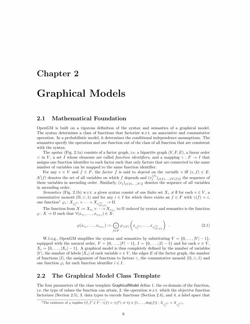


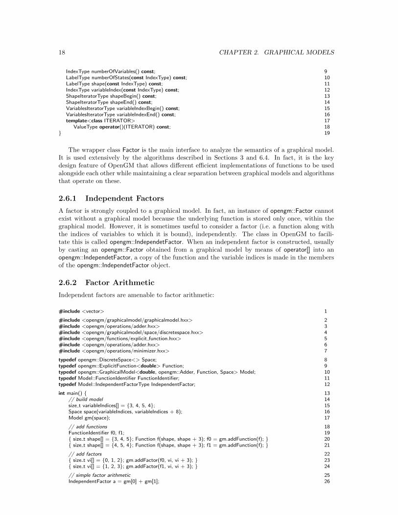


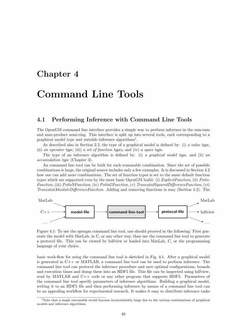


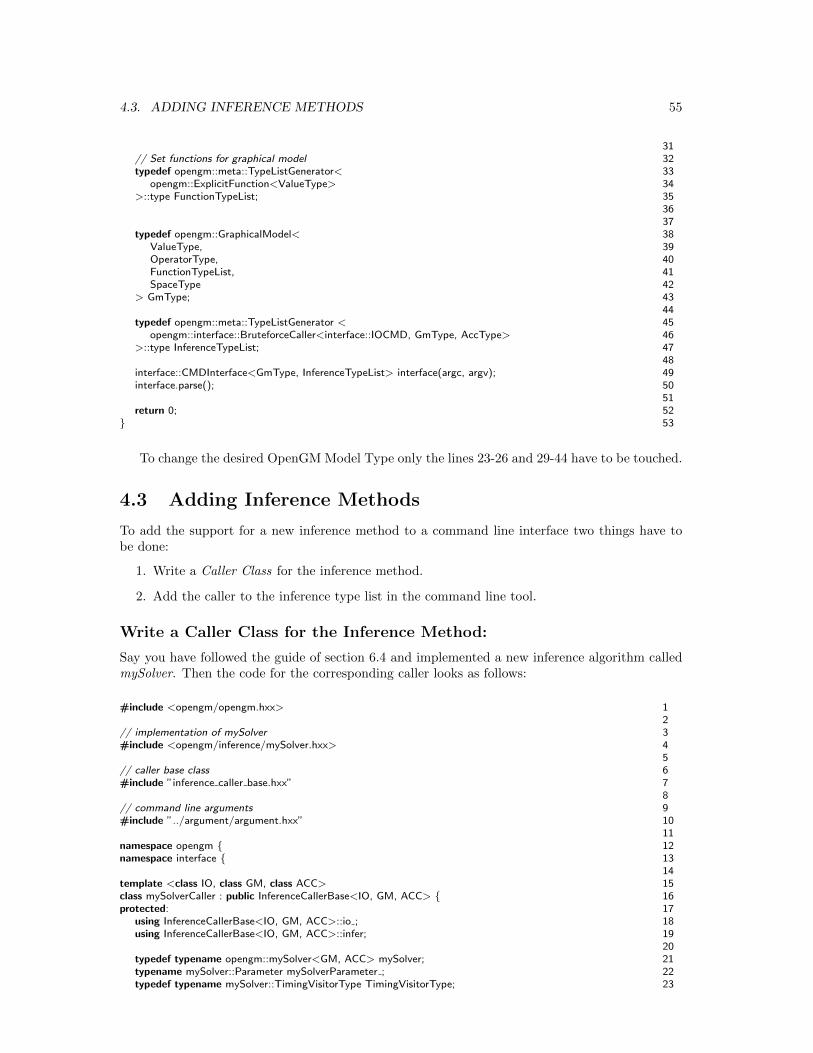

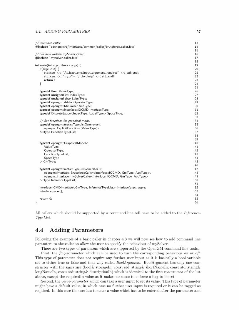

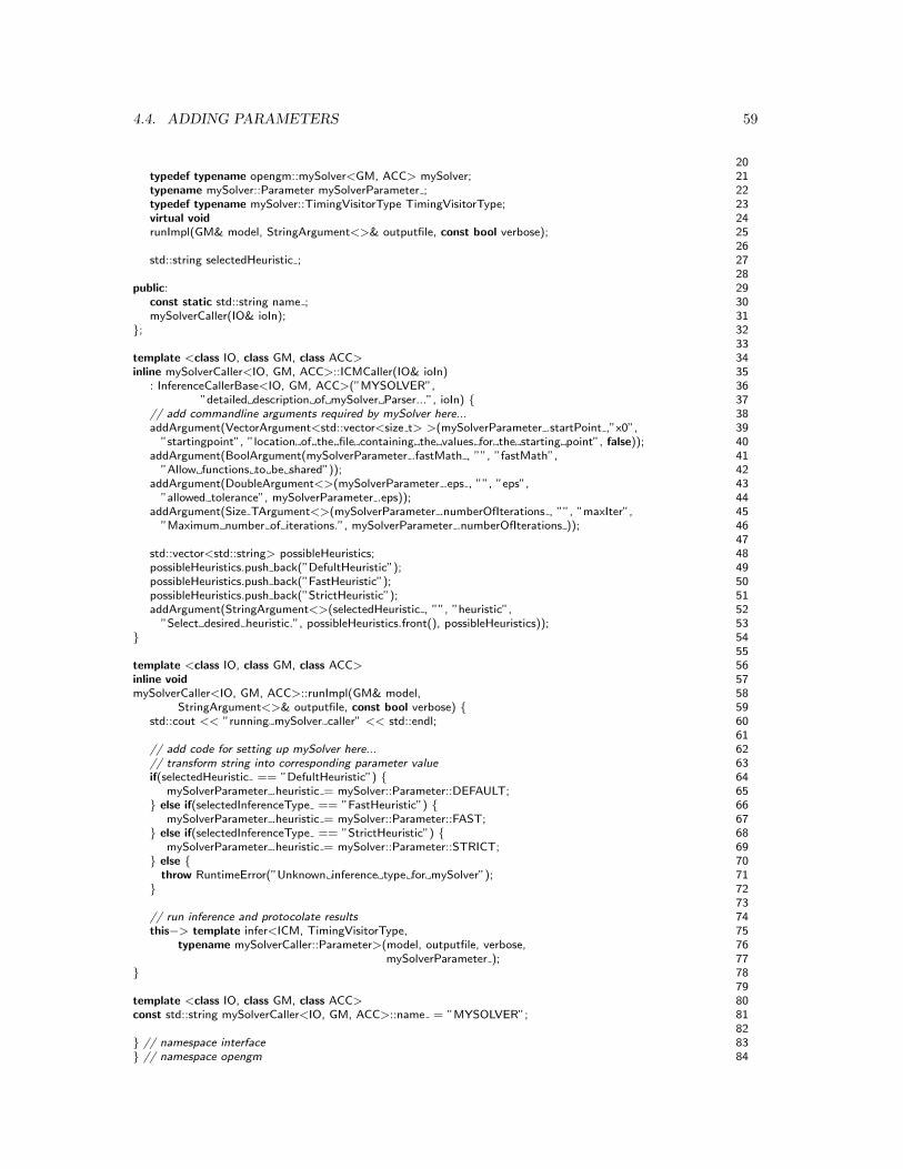


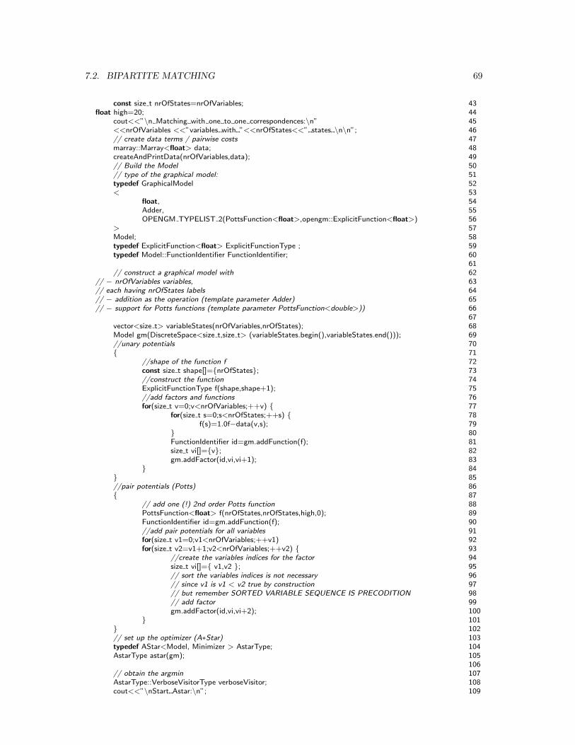
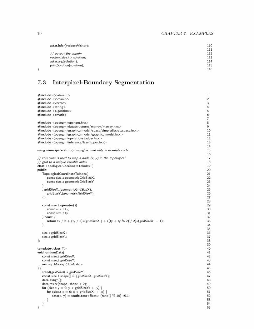
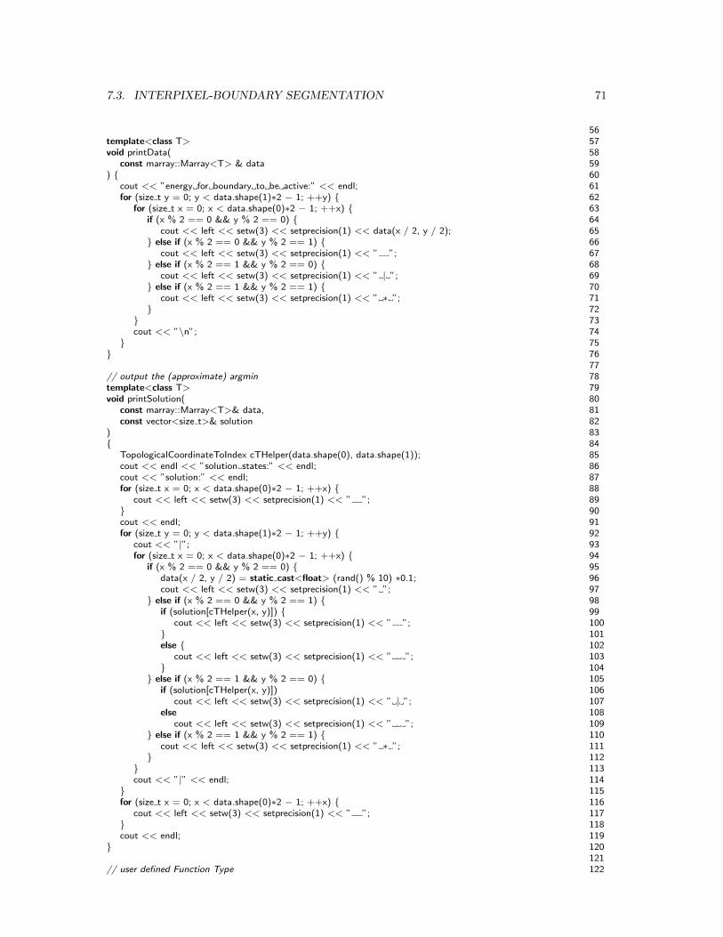


![Install Windows Cvs[1]](https://static.documents.pub/doc/80x56/577d21f81a28ab4e1e965107/install-windows-cvs1.jpg)


