Openness, Growth and Inflation: Evidence from South Korea Jang C. Jin Faculty of Business Administration The Chinese University of Hong Kong Shatin, New Territories Hong Kong Tel: (852) 2609-7902 Fax: (852) 2603-5104 Email: [email protected]
Transcript
Openness, Growth and Inflation: Evidence from South Korea
Jang C. JinFaculty of Business Administration
The Chinese University of Hong KongShatin, New Territories
provided further evidence that the measure of openness constructed by Sachs and Warner had robust
results on growth, whereas Harrison and Hanson (1999) failed to establish a robust result. Frankel and
Romer (1999) further constructed the geographic component of trade, and found a positive effect of
trade on real GDP per worker. Finally, the sample period used also matters. For the late 19th century,
O’Rourke (2000) provided evidence that increasing tariffs (and thus protection) was positively related
to growth. This would imply that increased openness slowed growth during this period.4
B. Openness and Inflation
The link between openness and inflation is based on the Barro-Gordon-type model that an
unanticipated monetary expansion can cause inflation to rise (Kydland and Prescott, 1977; Barro and
Gordon, 1983). Based on this model, Romer (1993) suggests that an inverse relationship between
openness and inflation arise through the impact of openness on policy-makers' incentives to pursue
expansionary policies. Unanticipated monetary expansion induces real exchange rates to depreciate.
The more a country's openness, the greater the harms of real depreciation, and thus less expansion of
monetary surprise is expected for more open economies. In this case, inflation falls.
Romer (1993) provided evidence that openness generally exerts a significant negative effect on
inflation in a broad cross-section of countries. Lane (1997) also found the inverse relationship between
openness and inflation across countries, based on the argument that the inverse relationship was due to
imperfect competition and price rigidity in non-traded sectors. Terra (1998) however argued that the
inverse relationship was due to indebted countries' need to raise revenue to repay their debts, and
significant negative relationships were found only for severely indebted countries.
7
C. Motivations
This brief review of the literature on openness and growth and openness and inflation relations
reveals three important considerations. First, many studies use cross-country data for LDCs. Some
studies use cross-industry data within a country. Little has been done for dynamics of the impact of
openness at a country level. Accordingly, this study differs importantly from others in the literature by
using time-series data for a developing country, Korea, to examine the dynamics of openness-growth
and openness-inflation relations simultaneously. The dynamics are examined through computation of
impulse response functions and forecast error variance decompositions, which are based on the moving-
average representation of the VAR model.
Second, many cross-section studies employ various measures of openness to find their
relationships with economic growth and inflation, but it is difficult to obtain long historical data for the
openness measures. Perhaps, this has led many studies in this area to the estimation of cross-country
averages of LDCs. For time-series analysis, the imports/GDP ratio is generally acknowledged in the
literature to be the best measure currently available (e.g. Romer, 1993). Alternative measures of
openness in financial markets, as well as in trade, will also be discussed in Section V.
Finally, as noted in Harrison (1996) and Edwards (1998), the issue of causality has not been
adequately addressed in this relevant literature. Although the Granger’s (1969) definition of causality
is not causality as it is usually understood, in practice, however, we would like to know whether a time
series openness precedes a time series GDP, or GDP precedes openness. This is the purpose of the
Granger causality test. Harrison (1996) briefly introduced causal orderings between openness and
growth. Yet it is widely known that the causal orderings are sensitive to the number of variables included
in the model. This study thus constructs a VAR as a small macro model of the Korean economy and
8employs IRFs and VDCs techniques to investigate the issues related to causal orderings between
openness and growth and openness and inflation.
III. Data Description and Model Specification
As noted earlier, the macroeconomic effects of openness are examined within the context of a
seven-variable VAR model. The model is specified and estimated using quarterly data for 1960:1-
1997:3. The period 1960:1-1963:1 is used as pre-sample data to generate the lags in the VAR, and
the model is estimated over the period 1963:2-1997:3. The beginning of our sample roughly coincides
with the period in which the Korean government placed increased reliance on international trade. The
end of our sample coincides with breaking out of 1997 financial crisis in Korea.
Quarterly data are used for two reasons. First, the size of our system requires quarterly data
in order to have enough degrees of freedom for estimation. The second reason is based on a desire to
minimize any problems with temporal aggregation (see Christiano and Eichenbaum, 1987) that might
arise with the use of annual data. In addition, the quarterly series is seasonally unadjusted. As pointed
out by Sims (1974) and Wallis (1974), seasonally adjusted data may create distortions in the
information content of the raw data and render valid inferences somewhat difficult. Several varied
procedures to remove seasonal components from the raw data may generate different series, depending
on the methodology and time periods used. Therefore, the use of seasonally unadjusted data is
warranted to avoid the smoothing problems inherent in the process of seasonal adjustment.
A vector autoregressive process of order p, VAR(p), for a system of k variables can be written
as
Xt = A + B(L) Xt + ut, (1)
9
where Xt is a k x 1 vector of system variables, A is a k x 1 vector of constants, B(L) is k x k matrix of
polynomials in the lag operator L, and ut is a k x 1 vector of serially uncorrelated white noise residuals.
As noted earlier, the standard Sims (1980) VAR is an unrestricted reduced-form approach and uses
a common lag length for each variable in each equation. That is, no restrictions are imposed on
coefficient matrices to be null, and the same lag length is used for all system variables.
Seven variables are included in the model: real gross domestic product (GDP) in 1990 prices
(y), the GDP deflator (P), the narrowly defined money supply (M), real government expenditures (g),
the imports/GDP ratio as an openness measure (OPEN), the industrial production index of industrial
countries as a foreign output shock measure (YSTAR), and the world commodity price index of all
exports as a foreign price shock variable (PSTAR). The data for all variables are obtained from the
international financial statistics.5
Following Romer (1993), the import share in GDP is used as a proxy for openness of an
economy. Since even protected economies like Japan have expanded exports to other countries, the
import share removes the export share from total trade. Unlike trade share in GDP, the import share
reveals import penetration that represents the degree of a country’s trade openness.
Since macroeconomic policies that are not directly related to trade may even cause a positive
correlation between openness and growth (e.g. Levine and Renelt, 1992), domestic monetary and fiscal
policy variables are included in the model as control variables and allow to influence aggregate demand.
M1 is used as a monetary policy variable. Real government expenditures are measured as the
consumption and investment of the consolidated central government in Korea and are deflated by the
GDP deflator (1990=100). It is important to include government expenditures in our model since the
fiscal policy variable can affect economic activity even if openness has no effect on output. Since
10monetary and fiscal policy variables can be correlated (e.g. debt monetization), macro effects due to
changes in government spending might be incorrectly attributed to money supply if government spending
were omitted from the model.
Because the Korean economy heavily depends on international trade, it is also important to
include variables like the foreign output and foreign price shocks. The foreign output shock variable,
YSTAR, is the industrial production index of industrial countries. The inclusion of YSTAR in our model
is similar to Genberg, Salemi, and Swoboda (1987) who used an index of European industrial
production to measure a foreign output shock variable in their study of the effects of foreign shocks on
the Swiss economy. The foreign price shock variable, PSTAR, is the world commodity price index of
all exports. A shock to PSTAR can be transmitted to the domestic economy through two different
channels. First, an increase in foreign prices may raise domestic exports but lower import demand.
Hence, the net exports may rise domestically. This transmission channel relates to an increase in
aggregate demand in which domestic output and prices rise through an increase in net exports. Second,
the foreign price shock may reduce aggregate supply because the import prices of intermediate goods
to be used in the domestic production process will be increased. Other things being equal, this would
tend to reduce domestic output and raise the price level.
Prior to estimation of the VAR, augmented Dickey-Fuller tests were employed to check for
first-order unit roots. These tests suggested that the first differences of the logs of YSTAR, PSTAR,
M, G, Y and P and the first differences of the level of OPEN should be used in specifying and estimating
the model. Based upon the arguments of Engle and Granger (1987), cointegration tests were also
performed for the seven variables that required differencing to achieve stationarity. Since no evidence
of cointegration was found, the system was estimated with differences of all system variables.
11IV. Basic Results
The sources of changes in the growth rates of output and of the price level are examined through
the computation of variance decompositions (VDCs) and impulse response functions (IRFs) which, in
turn, are based on the moving-average representations of the VAR model and reflect short-run dynamic
relationships between variables. The VDCs show the percent of the forecast error variance for each
variable that may be attributed to its own innovations and to fluctuations in other variables in the system.
The IRFs indicate the direction and size of the effect of a one standard deviation shock to one variable
on other system variables over time. Since model variables are converted to first differences prior to
estimation of the model, the VDCs and IRFs reported here indicate the effects of a shock to the
changes in openness on the growth rates of output and prices.
Since Runkle (1987) has argued that reporting VDCs and IRFs without standard errors is
similar to reporting regression coefficients without t-statistics, a Monte Carlo integration procedure is
employed to estimate standard errors for the VDCs and IRFs. One thousand draws are employed in
the Monte Carlo procedure. For the VDCs, the estimates of the proportion of forecast error variance
explained by each variable are judged to be significant if the estimate is at least twice the estimated
standard error. For the IRFs, a two standard deviation band is constructed around point estimates.
If this band include zero, the effect is considered insignificant.
Since the equations of the VAR contain only lagged values of the system variables, it is assumed
that the residuals of the VAR model are purged of the effects of past economic activity. Any
contemporaneous relations among the variables are reflected in the correlation of residuals across
equations. In this paper, the Choleski decomposition is used to orthogonalize the variance-covariance
matrix. In this approach, the variables are ordered in a particular fashion, and, in this way, some
structure is imposed in computation of the VDCs and IRFs. When a variable higher in the order changes,
12variables lower in the order are assumed to change. The extent of the change depends upon the
covariance of the variables higher in the order with that lower in the order.6
The variables are ordered as: YSTAR, PSTAR, OPEN, M, G, Y, P. Noting the potential
sensitivity of the results to variable orderings, theoretical considerations are used (e.g. Bernanke, 1986).
The placement of foreign output and price shocks first is based on the assumption that South Korea
is characterized as a small open economy so that current-period shocks to foreign output and prices are
allowed to influence domestic variables, but the domestic economy cannot contemporaneously affect
foreign shock variables. The placement of three domestic policy variables (OPEN, M, G) next is
consistent with the familiar textbook treatment of aggregate supply and aggregate demand in which
current period shocks to the policy variables can affect Y and P contemporaneously. Assumed in this
ordering is that current period shocks to Y have no contemporaneous effect on the three policy
variables. This is also consistent with the typical policy reaction functions in which the current values
of the policy variables depend only on the lagged values of domestic macro variables. Finally, the
placement of Y and P last allows the domestic output and prices to respond directly and indirectly to
contemporaneous shocks to domestic policy variables as well as foreign shocks.
The VAR order is set to twelve quarters to reduce serial correlation of the residuals. The
marginal significance levels of the Ljung-Box Q statistics range between 0.67 and 0.99. Choice of other
lag lengths merely reduces the significance levels of the Q statistics.
Figure 1 shows the point estimates of the IRFs, which are plotted with a dotted line, while the
solid lines represent a two standard deviation band around the point estimates. If this band excludes
zero, the effect is considered to be significant. For YSTAR and PSTAR innovations, the output effects
simply fluctuate around zero over horizons, while the price effects are observed to be positive and
significant at short horizons. In the case of OPEN innovation, the effect on output initially rises and the
13effect quickly becomes negative. The negative effect is significant at horizon of four quarters, and a
marginal significance is also observed at eight-quarter horizon. In the longer run, however, the effects
are not significantly different from zero. The price effects of OPEN are also initially negative and
significant, and significant negative effects are again observed at horizons of five, nine, eleven, and
thirteen quarters, although some positive effects appear significant at short horizons.
The significant, negative output effects of a shock to openness do not appear to support the new
growth theories that increasing openness helps the domestic economy to grow. The results also appear
to be at odds with the empirical findings of Lee (1995) and Kim (2000) for the Korean economy since
the short-run negative effects are in the opposite direction of those predicted by these studies. One
explanation for the negative effects found here has been suggested by Aitken and Harrison (1999)
based on a priori argument of Levine and Renelt (1992). The argument is that trade liberalization of
a developing country whose economic fundamentals are not very strong may discourage domestic
investment due to increased international competition, and its decrease would be greater than capital
inflows from abroad. In this case, net investment falls, as does aggregate demand. Therefore, increasing
openness has negative effects on the growth rates of output.
On the other hand, the observed negative price effects of openness are consistent with the
findings of Romer (1993), Lane (1997), and Terra (1998). The results appear to be consistent with
aggregate demand channel: a fall in net investment due to increased openness reduces aggregate demand
and hence the price level falls.
Other domestic policy shocks (M and G) also have non-trivial effects on economic growth and
inflation. Therefore, it is of interest to determine the relative importance of changes in openness to other
variable shocks. This information can be obtained by computing variance decompositions (VDCs) of
Y and P explained by other system variables.
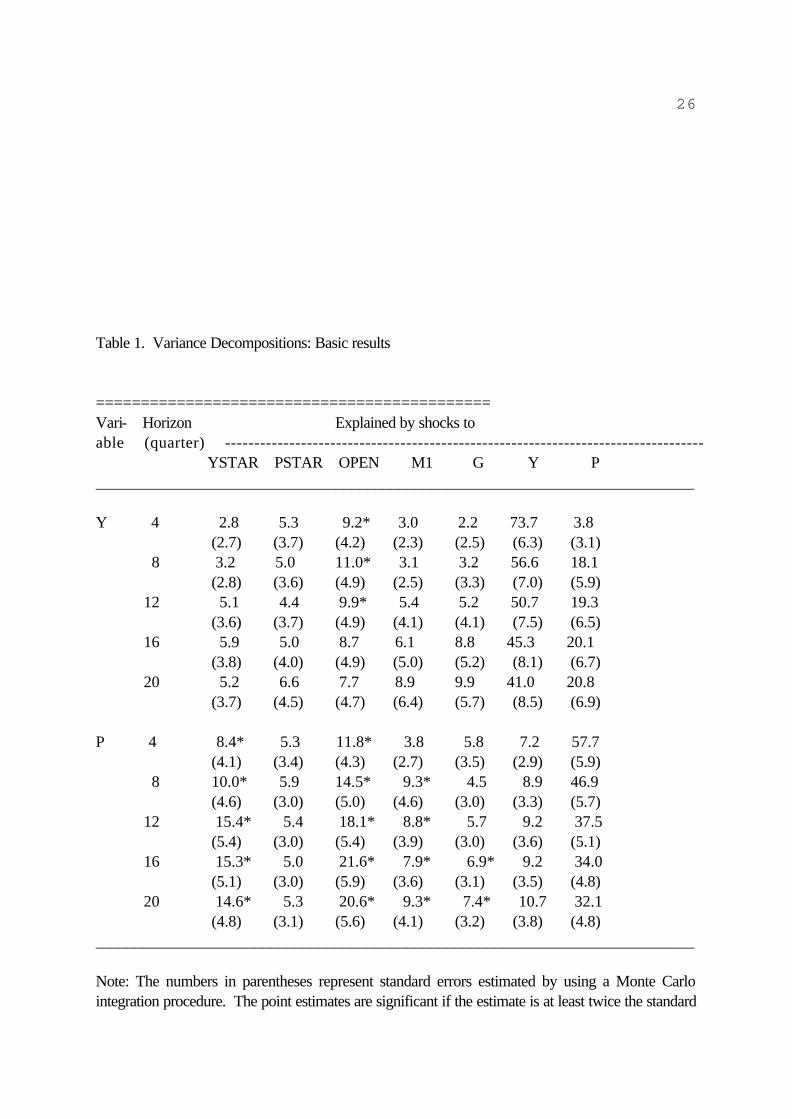
14Table 1 reports the VDC results. The estimated standard errors are in parentheses below the
point estimates. A * indicates that the point estimate is at least twice the standard error--our rule of
thumb for judging significance. VDCs at horizons of 4, 8, 12, 16, 20 quarters are shown in order to
convey a sense of the dynamics of the system. Only the effects on Y and P are shown in order to focus
upon the variables of central interest to the paper and to conserve space. The forecast error variance
of Y explained by OPEN innovation appears to be significant at short horizons, and the effect of
openness is greater than the effects of other variable shocks. The price effects of shock to openness
are also greater than the effects of other variable shocks, and the effects are significant at all horizons.
The results are generally consistent with the IRF results found in Figure 1. Furthermore, the price
effects of YSTAR innovations are relatively large and appear to be significant at all horizons. Shocks
to M and G also appear to be significant over longer horizons. The shocks emanating from domestic
policy variables such as M and G, as well as foreign output shocks, may transmit to the domestic
economy through the aggregate demand channel in which output and prices are affected by an increase
in aggregate demand. However, the results that price effects are greater and more significant than
output effects suggest that aggregate supply is relatively steep in Korea.
V. Alternative Specifications and Sensitivity Results
A. Lag Lengths
It is common practice to choose an ad hoc lag length when specifying distributed-lag models.
Because economic theory is often not very explicit about the lag lengths in time series relationships,
several VAR orders are employed to check on the robustness of the results.
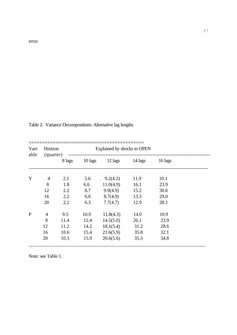
Table 2 shows the results of the VDCs with common lag lengths: 8, 10, 12, 14, and 16 quarters.
The 12-quarter lags employed for the basic results in Table 1 are used here as a benchmark lag length.
15 Although the sample period begins from 1960:1, estimation begins from 1962:2 1962:4, 1963:2,
1963:4, and 1964:2, respectively, due to different lag lengths used. The degrees of freedom reduce by
sixteen in each column, and thus the lag length longer than 16 quarters is not used here. The lag length
shorter than 8 quarters is not used as well since the serial correlation of residuals appears to be serious
with the use of shorter lags. Again, only the effects of OPEN on Y and P are shown to focus upon the
variables of central interest to the paper and to conserve space. The forecast error variance of output
explained by shocks to openness is small and insignificant for the 8-lag model, while the VDCs with 10-
quarter lags are all within one standard deviation of those in the 12-lag model. The results are more
convinced when longer lags are used. For 14-quarter and 16-quarter lags, the point estimates are even
greater than those in the 12-lag model. A similar pattern is observed for prices. When the lags smaller
than 12 quarters are used, the point estimates are relatively small; but the VDCs are large and significant
when longer lags are used. Thus, the significant output and price effects of openness are, with only a
few exceptions, qualitatively unchanged.
B. Variable Orderings
Another potential problem of this reduced-form VAR approach is that contemporaneous
correlation may exist among the residuals of the VAR model. For example, if the current value of the
residual in the first equation is correlated with the current value of the residual in the second equation,
the variable in the second equation is affected by changes in the variable of the first equation. Thus, a
pure innovation in a particular variable lower in order cannot be isolated. For this reason, innovation
accounting often uses the Choleski decomposition of the residual variance-covariance matrix to identify
orthogonal shocks to each variable. Although the Choleski decomposition orthogonalizes the VAR
residuals, it is generally recognized that innovation accounting results of the VAR are potentially sensitive
16to the ordering of system variables. Specifically, if there is substantial contemporaneous correlation,
variable ordering matters. When a variable higher in order changes, the variable lower in order also
changes. Consequently, innovation accounting results may be potentially sensitive to the ordering of
variables.
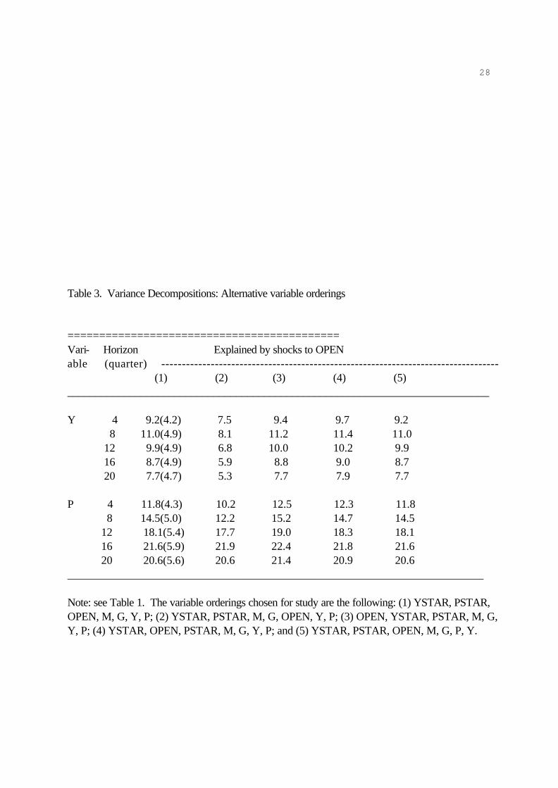
The orderings chosen for study are the following: (1) YSTAR, PSTAR, OPEN, M, G, Y, P;
(2) YSTAR, PSTAR, M, G, OPEN, Y, P; (3) OPEN, YSTAR, PSTAR, M, G, Y, P; (4) YSTAR,
OPEN, PSTAR, M, G, Y, P; and (5) YSTAR, PSTAR, OPEN, M, G, P, Y. As noted earlier, the
benchmark ordering (1) is designed to be consistent with a model in which the IS-LM model underlies
aggregate demand and where output and the price level respond to current innovations in domestic
policy variables as well as foreign shock variables. In ordering (2), OPEN is allowed affected by
contemporaneous shocks to M and G. This is the case that monetary and fiscal policy shocks may
cause large foreign exchange depreciation; the depreciation would increase exports but decrease
imports; and thus the imports/GDP ratio, which is our openness measure, would be affected.
Furthermore, this ordering is consistent with the set of structural models in which foreign shocks as well
as domestic policy variable shocks have both direct and perhaps indirect contemporaneous effects on
OPEN. Ordering (3), however, places OPEN first in the ordering, based on the assumption that any
contemporaneous effects flow from the openness variable to all other model variables. Ordering (4)
places the openness variable next to YSTAR but prior to PSTAR. Ordering (5) is the same as ordering
(1) except that the ordering of Y and P is switched.
The VDCs for all different orderings are reported in Table 3. Although OPEN is ordered in
several different places, the results are essentially unchanged. The point estimates in orderings (2) - (5)
are all within one standard deviation of those in column (1).7 The VDCs, thus, indicate that significant
effects of openness on the macroeconomy are not materially changed due to variable orderings.
17
C. Openness Measures
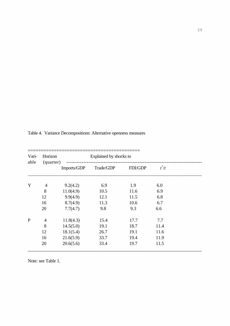
Table 4 further reports the VDC results, employing alternative openness measures. In addition
to the imports/GDP ratio, the trade/GDP ratio also reveals the degree of a country’s openness to world
trade: the more open a domestic economy is, the less is the restriction in world trade, and the higher is
the trade share in GDP. This trade share in GDP is most commonly used in the related literature (e.g.
Harrison, 1996). The results found in column (2) are similar to our earlier findings in column (1).
While both import shares and trade shares in GDP represent openness to trade, other openness
measures used in columns (3) and (4) represent the openness of financial markets. As indicated in
Levine and Renelt (1992), openness and growth relations may occur through investment, and hence
increasing openness may raise long-run growth only insofar as openness provides greater access to
investment goods. When countries begin to liberalize barriers in financial markets, foreign direct
investment (FDI) will be stimulated from abroad. Thus, the FDI/GDP ratio is used in column (3) as a
proxy for financial market openness. Column (4) further employs interest rate differentials in which a
large gap between domestic and foreign interest rates represents a small degree of openness. For these
two measures, our sample begins in 1977:1 since this is the earliest date for which we can obtain the
FDI and interest rate series. The beginning of our sample roughly coincides with the period in which
the Korean government placed increased reliance on FDI and the sale of bonds to foreign investors.
Ideally, a debt series that is held by foreigners as a percentage of total debt would also be preferred,
but no series of this type is available quarterly. Because sample periods are relatively short in columns
(3) and (4), eight rather than 12 lags are used for estimation. It is observed that changes in output and
price effects are all within one standard deviation of those in column (1), while the effects in column (4)
particularly shrink.
18Furthermore, the IRF results are presented in Figure 2. The significant short-run effects of
financial market openness are found to be negative on the growth rates of output and of the price level.
Trade openness measures are also observed to have significant negative effects on Y and P in the short
run. One exception is the insignificant response of P to shocks to the imports/GDP ratio.8 Other than
that, the significant short-run effects are all negative.
VI. Concluding Remarks
This paper has examined the effects of increasing openness on the growth rates of output and
of the price level in Korea. Unlike most studies that concentrate on the estimation of cross-country or
cross-industry averages, this study focuses upon the dynamics of openness-growth and openness-
inflation relations for a rapidly growing economy, one in which rapid growth has been accompanied by
a persistent government intervention in international trade and financial markets. This study also differs
from others in the literature by employing VAR techniques that are of a less restrictive empirical
framework. The framework of analysis is a seven-variable VAR model that consists of output, the price
level, the money supply, real government spending, foreign output and foreign price shocks, and
openness measures.
The effects of changes in openness on economic growth and inflation rates are evaluated
through the computation of impulse response functions and variance decompositions. The impulse
response functions indicate that significant effects of a shock to openness on the growth rates of output
and of the price level are negative. The variance decompositions also indicate that the effects of
openness on these variables are significant and greater than the effects of other variable shocks. The
results are, in general, robust across lag lengths, variable orderings, and alternative openness measures.
The impulse response functions further indicate that proxies for financial market openness, as well as
19trade openness, have negative impacts on the growth rates of output and of the price level.
In the new growth theories, openness improves productivity and hence economic growth. In
the short run, output is found affected negatively by openness measures although there are no longer-run
effects. The results do not appear to support the new growth theories, since the short-run negative
effects are in the opposite direction of those predicted by the new growth theories. The price effect of
openness is also found negative. The significant negative effects of increasing openness on output
growth and inflation appear to be consistent with the argument of Aitken and Harrison (1999) and
Levine and Renelt (1992) that the increased international competition due to openness may cause
domestic investment to decline and its decrease would be greater than an increase in capital inflows from
abroad. In this case, net investment falls, so does aggregate demand.
20
FOOTNOTES
1. Average annual growth rates of real GDP and GDP deflator since 1960 are 8.8% and 13.3%,
respectively, in South Korea.
2. The drawback of the VAR, of course, is that it is difficult to distinguish sharply among different
structural models, since the VAR technique is a reduced-form approach. Cooley and LeRoy
(1985) and Leamer (1985) have pointed out the limitation of the VAR approach.
3. Here, tariffs are assumed to be reduced on final goods, not intermediate inputs. Suppose tariffs are
reduced on intermediate inputs, then the tariff cut reduces the import price of inputs, which, in turn,
reduces costs of production to boost output. This type of effect would raise aggregate supply.
4. For the late 20th century, however, Edwards (1992, 1993, 1998), Lee (1993, 1995), Sachs and
Warner (1995), Sala-i-Martin (1997), and Kim (2000), among others, found that tariff rates had
negative effects on the rate of growth.
5. For more details, see the data appendix.
6. Several alternatives to the Choleski decomposition have been suggested. Bernanke (1986) uses
the residuals from a structural model as 'fundamental' shocks, and Blanchard and Quah (1989) use
long-run constraints that are, in principle, consistent with alternative structural models as fundamental
shocks. However, unless the structural models are just identified, in general, there will be
correlation across equations in the residuals of the structural model, and the issue of an appropriate
ordering arises again.
217. Note that, for ordering (5), the point estimates are identical to those in column (1) since the order
of OPEN is unchanged.
8. The results were slightly different from those in Figure 1 because here in Figure 2 eight lags were
used rather than twelve to be consistent with others.
22
REFERENCES
Aitken, Brian J. and Harrison, Ann E. (1999) “Do Domestic Firms Benefit from Direct Foreign
Investment? Evidence from Venezuela,” American Economic Review 89, 605-618.
Barro, Robert (1991) "Economic Growth in a Cross Section of Countries," Quarterly Journal of
Economics 106, 407-443.
Barro, Robert and Gordon, David (1983) "Rules, Discretion and Reputation in a Model of Monetary
Policy," Journal of Monetary Economics XII, 101-121.
Barro, Robert and Sala-i-Martin, Xavier (1995) Economic Growth, New York: McGraw-Hill.
Batra, Ravi (1992) "The Fallacy of Free Trade," Review of International Economics, 19-31.
Batra, Ravi and Beladi, Hamid (1996) “Gains from Trade in a Deficit-Ridden Economy,” Journal of
Institutional and Theoretical Economics 152, 540-554.
Bernanke, B. S. (1986) "Alternative Explanations of the Money-income Correlation," Carnegie-
Rochester Conference Series on Public Policy 25, 49-99.
Blanchard, O. J. and Quah, D. (1989) "The Dynamic Effects of Aggregate Demand and Supply
Disturbances," American Economic Review 79, 655-673.
Christiano, L.J. and Eichenbaum, M. (1987) "Temporal Aggregation and Structural Inference in
Macroeconometrics, Carnegie-Rochester Conference Series on Public Policy 26, 63-130.
Cooley, T. F. and LeRoy, S. F. (1985) "Atheoretical Macroeconomics: A Critique," Journal of
Monetary Economics 16, 283-308.
23Edwards, S. (1992) "Trade Orientation, Distortions, and Growth in Developing Countries," Journal of
Development Economics 39, 31-57.
Edwards, S. (1993) "Openness, Trade Liberalization and Growth in Developing Countries," Journal of
Economic Literature 31, 1358-1393.
Edwards, S. (1998) “Openness, Productivity and Growth: What Do We Really Know?” Economic
Journal 108, 383-398.
Engle, R. F. and Granger, C.W.J. (1987) "Cointegration and Error Correction: Representation,
Estimation, and Testing," Econometrica 55, 251-276.
Frankel J. A. and Romer, D. (1999) “Does Trade Cause Growth?” American Economic Review 89,
379-399.
Genberg, H., Salemi, M. K., and Swoboda, A. (1987) "The Relative Importance of Foreign and
Domestic Disturbances for Aggregate Fluctuations in the Open Economy: Switzerland, 1964-
81," Journal of Monetary Economics 19, 45-67.
Granger, C. W. J. (1969) “Investigating Causal Relations by Econometric Models and Cross-spectral
Methods,” Econometrica, 424-438.
Grossman, G. M. and Helpman E. (1991) Innovation and Growth in the Global Economy, Cambridge,
Massachusetts: MIT Press.
Harrison, A. (1996) "Openness and Growth: A Time-series, Cross-country Analysis for Developing
Countries," Journal of Development Economics 48, 419-447.
Harrison, A. and Hanson G. (1999) “Who Gains from Trade Reform? Some Remaining Puzzles,”
Journal of Development Economics 59, 125-154.
Kim, Euysung (2000) “Trade Liberalization and Productivity Growth in Korean Manufacturing
Industries: Price Protection, Market Power, and Scale Efficiency,” Journal of Development
24Economics 62, 55-83.
Kydland, Finn, and Prescott, Edward (1977) "Rules Rather than Discretion: The Inconsistency of
Optimal Plans," Journal of Political Economy LXXXV, 473-492.
Lane, Philip R. (1997) "Inflation in Open Economies," Journal of International Economics 42, 327-347.
Leamer, Edward E. (1985) "Vector Autoregressions for Causal Inference?" Carnegie-Rochester
Conference Series on Public Policy 22, 255-303.
Leamer, Edward E. (1995) "A Trade Economist's View of U.S. Wages and Globalization," Brookings
Conference Proceedings.
Lee, Jong Wha (1993) “International Trade, Distortions, and Long-Run Economic Growth,”
International Monetary Fund Staff Papers 40(2), 299-328.
Lee, Jong Wha (1995) “Government Interventions and Productivity Growth in Korean Manufacturing
Industries,” NBER Working Paper No. 5060.
Levine, R. and Renelt, D. (1992) "A Sensitivity Analysis of Cross-Country Growth Regressions,"
American Economic Review 82, 942-963.
Lucas, Robert E. (1988) “On the Mechanics of Economic Development,” Journal of Monetary
Economics 22(1), 3-42.
O’Rourke, K. H. (2000) “Tariffs and Growth in the Late 19th Century,” Economic Journal 110, 456-
483.
Romer, David (1993) "Openness and Inflation: Theory and Evidence," Quarterly Journal of Economics
108, 869-903.
Romer, David (1998) "A New Assessment of Openness and Inflation: Reply," Quarterly Journal of
Economics 113, 649-652.
Romer, Paul M. (1986) “Increasing Returns and Long Run Growth,” Journal of Political Economy 94
25(5), 1002-1037.
Romer, Paul M. (1992) “Two Strategies for Economic Development: Using Ideas and Producing
Ideas,” World Bank Annual Conference on Economic Development, Washington, DC, The
World Bank.
Sachs, J. and Warner, A. (1995) “Economic Reform and the Process of Global Integration,”
Brookings Papers Economic Activity 1, 1-117.
Sala-i-Martin, X. (1997) “I Just Ran Two Million Regressions,” American Economic Review 87, 178-
183.
Sims, Christopher A. (1974) "Seasonality in Regression," Journal of American Statistical Association,
618-626.
Solow, R. M. (1957) "Technical Change and the Aggregate Production Function," Review of
Economics and Statistics 39, 312-320.
Terra, Cristina T. (1998) "Openness and Inflation: A New Assessment," Quarterly Journal of
Economics 113, 641-648.
Wallis, K.F. (1974) "Seasonal Adjustment and Relations between Variables," Journal of American
Statistical Association, 18-34.
26
Table 1. Variance Decompositions: Basic results
============================================Vari- Horizon Explained by shocks toable (quarter) ---------------------------------------------------------------------------------- YSTAR PSTAR OPEN M1 G Y P___________________________________________________________________________
Note: The numbers in parentheses represent standard errors estimated by using a Monte Carlointegration procedure. The point estimates are significant if the estimate is at least twice the standard
27
error.
Table 2. Variance Decompositions: Alternative lag lengths
===========================================Vari- Horizon Explained by shocks to OPENable (quarter) --------------------------------------------------------------------------------- 8 lags 10 lags 12 lags 14 lags 16 lags___________________________________________________________________________
Note: see Table 1. The variable orderings chosen for study are the following: (1) YSTAR, PSTAR,OPEN, M, G, Y, P; (2) YSTAR, PSTAR, M, G, OPEN, Y, P; (3) OPEN, YSTAR, PSTAR, M, G,Y, P; (4) YSTAR, OPEN, PSTAR, M, G, Y, P; and (5) YSTAR, PSTAR, OPEN, M, G, P, Y.
29
Table 4. Variance Decompositions: Alternative openness measures
Note: Point estimates of the IRFs are plotted with a dotted line, while solid lines represent a twostandard deviation band around the point estimate.Figure 1 (continued)
32
Figure 2. Impulse Responses: Alternative Openness Measures
33
Note: Point estimates of the IRFs are plotted with a dotted line, while solid lines represent a twostandard deviation band around the point estimate.Figure 2 (continued)
34
DATA APPENDIX
Quarterly data were obtained from the International Financial Statistics. The numbers in
brackets are the IFS code for the variables used. The sample period with exception of those discussed
below is from 1960:1 to 1997:3.
Y: real gross domestic product (GDP) in 1990 prices [99b.p], billions of Korean won.
P: GDP deflator, 1990=100, generated by the ratios of nominal GDP to real GDP.
M: narrowly defined money supply [34], billions of Korean won.
G: real government expenditures [82], billions of Korean won, deflated by the GDP deflator
(1990=100).
YSTAR: industrial production index of industrial countries, 1990=100, obtained from the
35
industrial countries table [11066.I].
PSTAR: world commodity price index of all exports, 1990=100, obtained from the world table
[00176AXD].
OPEN: imports/GDP ratio. Since commodity imports in Korea [71.d] were measured in
millions of U.S. dollars, nominal exchange rates, period average [rf] were used to convert the imports
in U.S. dollars to Korean won. Other openness measures used were as follows. Trade/GDP: total
trade converted to Korean won was divided by nominal GDP. FDI/GDP: foreign direct investment in
Korea [78bed], millions of U.S. dollars, was again converted to Korean won by using the nominal
exchange rates. r*/r: SDR interest rates [99260S] were used as a proxy for foreign interest rates (r*),
and the money market rate of interest [60B] in Korea was used for domestic interest rates (r). For the
FDI and interest rate series, the sample period begins from 1977:1 to 1997:3 due to data availability