Heizer Operations Management 10th edition Module C
20
Quantitative Module L EARNING O BJECTIVES When you complete this module you should be able to IDENTIFY OR DEFINE: Transportation modeling Facility location analysis EXPLAIN OR BE ABLE TO USE: Northwest-corner rule Stepping-stone method C Transportation Models Module Outline TRANSPORTATION MODELING DEVELOPING AN INITIAL SOLUTION The Northwest-Corner Rule The Intuitive Lowest-Cost Method THE STEPPING-STONE METHOD SPECIAL ISSUES IN MODELING Demand Not Equal to Supply Degeneracy SUMMARY KEY TERMS USING SOFTWARE TO SOLVE TRANSPORTATION PROBLEMS SOLVED PROBLEMS INTERNET AND STUDENT CD-ROM EXERCISES DISCUSSION QUESTIONS PROBLEMS INTERNET HOMEWORK PROBLEMS CASE STUDY: CUSTOM VANS, INC. ADDITIONAL CASE STUDIES BIBLIOGRAPHY
Transcript
Quantitative Module
LEARNING OBJECTIVESWhen you complete this module youshould be able to
IDENTIFY OR DEFINE:
Transportation modeling
Facility location analysis
EXPLAIN OR BE ABLE TO USE:
Northwest-corner rule
Stepping-stone method
CTransportation Models
Module OutlineTRANSPORTATION MODELING
DEVELOPING AN INITIAL SOLUTION
The Northwest-Corner Rule
The Intuitive Lowest-Cost Method
THE STEPPING-STONE METHOD
SPECIAL ISSUES IN MODELING
Demand Not Equal to Supply
Degeneracy
SUMMARY
KEY TERMS
USING SOFTWARE TO SOLVE TRANSPORTATION
PROBLEMS
SOLVED PROBLEMS
INTERNET AND STUDENT CD-ROM EXERCISES
DISCUSSION QUESTIONS
PROBLEMS
INTERNET HOMEWORK PROBLEMS
CASE STUDY: CUSTOM VANS, INC.
ADDITIONAL CASE STUDIES
BIBLIOGRAPHY
HEIZMX0C_013185755X.QXD 5/4/05 2:44 PM Page 723
724 MO D U L E C TR A N S P O RTAT I O N MO D E L S
TransportationmodelingAn iterative procedure forsolving problems thatinvolves minimizing thecost of shipping productsfrom a series of sources toa series of destinations.
The problem facing rental companies like Avis, Hertz, and National is cross-country travel. Lots of it. Cars rented in
New York end up in Chicago, cars from L.A. come to Philadelphia, and cars from Boston come to Miami. The scene
is repeated in over 100 cities around the U.S. As a result, there are too many cars in some cities and too few in
others. Operations managers have to decide how many of these rentals should be trucked (by costly auto carriers)
from each city with excess capacity to each city that needs more rentals. The process requires quick action for the
most economical routing; so rental car companies turn to transportation modeling.
Because location of a new factory, warehouse, or distribution center is a strategic issue with sub-stantial cost implications, most companies consider and evaluate several locations. With a widevariety of objective and subjective factors to be considered, rational decisions are aided by a num-ber of techniques. One of those techniques is transportation modeling.
The transportation models described in this module prove useful when considering alternativefacility locations within the framework of an existing distribution system. Each new potential plant,warehouse, or distribution center will require a different allocation of shipments, depending on itsown production and shipping costs and the costs of each existing facility. The choice of a new loca-tion depends on which will yield the minimum cost for the entire system
TRANSPORTATION MODELINGTransportation modeling finds the least-cost means of shipping supplies from several origins toseveral destinations. Origin points (or sources) can be factories, warehouses, car rental agencies likeAvis, or any other points from which goods are shipped. Destinations are any points that receivegoods. To use the transportation model, we need to know the following:
1. The origin points and the capacity or supply per period at each.2. The destination points and the demand per period at each.3. The cost of shipping one unit from each origin to each destination.
The transportation model is actually a class of the linear programming models discussed inQuantitative Module B. As it is for linear programming, software is available to solve transporta-tion problems. To fully use such programs, though, you need to understand the assumptions thatunderlie the model. To illustrate one transportation problem, in this module we look at a companycalled Arizona Plumbing, which makes, among other products, a full line of bathtubs. In ourexample, the firm must decide which of its factories should supply which of its warehouses.Relevant data for Arizona Plumbing are presented in Table C.1 and Figure C.1. Table C.1 shows,for example, that it costs Arizona Plumbing $5 to ship one bathtub from its Des Moines factory toits Albuquerque warehouse, $4 to Boston, and $3 to Cleveland. Likewise, we see in Figure C.1
HEIZMX0C_013185755X.QXD 5/4/05 2:44 PM Page 724
DE V E L O P I N G A N IN I T I A L SO L U T I O N 725
TABLE C.1 �
Transportation Costs perBathtub for ArizonaPlumbing
that the 300 units required by Arizona Plumbing’s Albuquerque warehouse may be shipped in var-ious combinations from its Des Moines, Evansville, and Fort Lauderdale factories.
The first step in the modeling process is to set up a transportation matrix. Its purpose is to summa-rize all relevant data and to keep track of algorithm computations. Using the information displayed inFigure C.1 and Table C.1, we can construct a transportation matrix as shown in Figure C.2.
DEVELOPING AN INITIAL SOLUTIONOnce the data are arranged in tabular form, we must establish an initial feasible solution to the prob-lem. A number of different methods have been developed for this step. We now discuss two of them,the northwest-corner rule and the intuitive lowest-cost method.
Albuquerque(300 unitsrequired)
Des Moines(100 unitscapacity)
Evansville(300 unitscapacity)
Cleveland(200 unitsrequired)
Boston(200 unitsrequired)
Fort Lauderdale(300 unitscapacity)
FIGURE C.1 �
Transportation Problem
FromTo
Des Moines
$5
Albuquerque
Evansville
$8
Fort Lauderdale
$9
$4
Boston
$4
$7
$3
Cleveland
$3
$5
Factorycapacity
Warehouserequirement 300 200 200 700
300
300
100
Clevelandwarehouse demand
Cost of shipping 1 unit from FortLauderdale factory to Boston warehouse
Total demandand total supply
Cellrepresenting a possiblesource-to-destinationshippingassignment(Evansvilleto Cleveland)
Des Moinescapacityconstraint
FIGURE C.2 �
Transportation Matrix forArizona Plumbing
HEIZMX0C_013185755X.QXD 5/4/05 2:44 PM Page 725
Example C1The northwest-corner rule
Northwest-corner ruleA procedure in thetransportation modelwhere one starts at theupper left-hand cell of a table (the northwestcorner) andsystematically allocatesunits to shipping routes.
726 MO D U L E C TR A N S P O RTAT I O N MO D E L S
FromTo
(D) Des Moines
(E) Evansville
(F) Fort Lauderdale
$9
$4 $3
(A)Albuquerque
(B)Boston
(C)Cleveland
$3
Factorycapacity
Warehouserequirement 300 200 200 700
300
300
100
200
100
100
100
200
Means that the firm is shipping 100bathtubs from Fort Lauderdale to Boston
$5
$8 $4
$7 $5
FIGURE C.3 �Northwest-CornerSolution to ArizonaPlumbing Problem
TABLE C.2 � Computed Shipping Cost
ROUTE
FROM TO TUBS SHIPPED COST PER UNIT TOTAL COST
D A 100 $5 $ 500E A 200 8 1,600E B 100 4 400F B 100 7 700F C 200 5 $1,000
Total: $4,200
The northwest-corner ruleis easy to use, but it totallyignores costs.
Intuitive methodA cost-based approachto finding an initial solutionto a transportationproblem.
The Northwest-Corner RuleThe northwest-corner rule requires that we start in the upper left-hand cell (or northwest corner) ofthe table and allocate units to shipping routes as follows:
1. Exhaust the supply (factory capacity) of each row (e.g., Des Moines: 100) before movingdown to the next row.
2. Exhaust the (warehouse) requirements of each column (e.g., Albuquerque: 300) beforemoving to the next column on the right.
3. Check to ensure that all supplies and demands are met.
Example C1 applies the northwest-corner rule to our Arizona Plumbing problem.
The solution given is feasible because it satisfies all demand and supply constraints.
The Intuitive Lowest-Cost MethodThe intuitive method makes initial allocations based on lowest cost. This straightforward approachuses the following steps:
1. Identify the cell with the lowest cost. Break any ties for the lowest cost arbitrarily.2. Allocate as many units as possible to that cell without exceeding the supply or demand.
Then cross out that row or column (or both) that is exhausted by this assignment.3. Find the cell with the lowest cost from the remaining (not crossed out) cells.4. Repeat steps 2 and 3 until all units have been allocated.
In Figure C.3 we use the northwest-corner rule to find an initial feasible solution to the Arizona Plumbingproblem. To make our initial shipping assignments, we need five steps:
1. Assign 100 tubs from Des Moines to Albuquerque (exhausting Des Moines’s supply).2. Assign 200 tubs from Evansville to Albuquerque (exhausting Albuquerque’s demand).3. Assign 100 tubs from Evansville to Boston (exhausting Evansville’s supply).4. Assign 100 tubs from Fort Lauderdale to Boston (exhausting Boston’s demand).5. Assign 200 tubs from Fort Lauderdale to Cleveland (exhausting Cleveland’s demand and Fort
Lauderdale’s supply).
The total cost of this shipping assignment is $4,200 (see Table C.2).
HEIZMX0C_013185755X.QXD 5/4/05 2:44 PM Page 726
TH E ST E P P I N G-STO N E ME T H O D 727
Stepping-stone methodAn iterative technique for moving from an initialfeasible solution to anoptimal solution in thetransportation method.
FromTo
(D) Des Moines
(E) Evansville
(F) Fort Lauderdale
Warehouse requirement
(A)Albuquerque
(B)Boston
(C)Cleveland
300 200 200 700
300
300
100
100
100
200
$9
$8
$5 $4
$4
$7
$3
$3
$5
300
Factorycapacity
Second, cross out column C afterentering 100 units in this $3 cellbecause column C is satisfied.
First, cross out top row (D) afterentering 100 units in $3 cellbecause row D is satisfied.
Finally, enter 300 units in the only remaining cell to complete the allocations.
Third, cross out row E and column B afterentering 200 units in this $4 cell because a total of 300 units satisfies row E.
FIGURE C.4 � Intuitive Lowest-Cost Solution to Arizona Plumbing Problem
When we use the intuitive approach on the data in Figure C.2 (rather than the northwest-corner rule) for ourstarting position we obtain the solution seen in Figure C.4.
The total cost of this approach = $3(100) + $3(100) + $4(200) + $9(300) = $4,100.
(D to C) (E to C) (E to B) (F to A)
While the likelihood of a minimum-cost solution does improve with the intuitive method, we wouldhave been fortunate if the intuitive solution yielded the minimum cost. In this case, as in the north-west-corner solution, it did not. Because the northwest-corner and the intuitive lowest-costapproaches are meant only to provide us with a starting point, we often will have to employ an addi-tional procedure to reach an optimal solution.
THE STEPPING-STONE METHODThe stepping-stone method will help us move from an initial feasible solution to an optimal solu-tion. It is used to evaluate the cost effectiveness of shipping goods via transportation routes not cur-rently in the solution. When applying it, we test each unused cell, or square, in the transportationtable by asking: What would happen to total shipping costs if one unit of the product (for example,one bathtub) was tentatively shipped on an unused route? We conduct the test as follows:
1. Select any unused square to evaluate.2. Beginning at this square, trace a closed path back to the original square via squares that are
currently being used (only horizontal and vertical moves are permissible). You may, how-ever, step over either an empty or an occupied square.
3. Beginning with a plus (+) sign at the unused square, place alternating minus signs and plussigns on each corner square of the closed path just traced.
4. Calculate an improvement index by first adding the unit-cost figures found in each squarecontaining a plus sign and then by subtracting the unit costs in each square containing aminus sign.
5. Repeat steps 1 through 4 until you have calculated an improvement index for all unusedsquares. If all indices computed are greater than or equal to zero, you have reached an opti-mal solution. If not, the current solution can be improved further to decrease total shippingcosts.
Example C3 illustrates how to use the stepping-stone method to move toward an optimal solu-tion. We begin with the northwest-corner initial solution developed in Example 1.
Example C2The intuitive lowest-costapproach
Example C3Checking unused routeswith stepping stone
We can apply the stepping-stone method to the Arizona Plumbing data in Figure C.3 (see Example 1) toevaluate unused shipping routes. As you can see, the four currently unassigned routes are Des Moines toBoston, Des Moines to Cleveland, Evansville to Cleveland, and Fort Lauderdale to Albuquerque.
Steps 1 and 2. Beginning with the Des Moines–Boston route, first trace a closed path using only currentlyoccupied squares (see Figure C.5). Place alternating plus and minus signs in the corners of this path. In the
HEIZMX0C_013185755X.QXD 5/4/05 2:44 PM Page 727
728 MO D U L E C TR A N S P O RTAT I O N MO D E L S
Result of proposed shift in allocation = 1 $4 – 1 $5 + 1 $8 – 1 $4 = + $3
Evaluation of Des Moines to Boston square
FromTo
(D) Des Moines
(E) Evansville
(F) Fort Lauderdale
$9
$3
(A)Albuquerque
(B)Boston
(C)Cleveland
$3
Factorycapacity
Warehouserequirement 300 200 200 700
300
300
100
200
100
100
100
200
$5
$8 $4
$7 $5
$4Start
201200
$8 99 $4
99$5 1 $4100
100
� � ��
FIGURE C.5 � Stepping-Stone Evaluation of Alternative Routes forArizona Plumbing
upper left square, for example, we place a minus sign because we have subtracted 1 unit from the original 100.Note that we can use only squares currently used for shipping to turn the corners of the route we are tracing.Hence, the path Des Moines–Boston to Des Moines–Albuquerque to Fort Lauderdale–Albuquerque to FortLauderdale–Boston to Des Moines–Boston would not be acceptable because the Fort Lauderdale–Albuquerquesquare is empty. It turns out that only one closed route exists for each empty square. Once this one closed pathis identified, we can begin assigning plus and minus signs to these squares in the path.
Step 3. How do we decide which squares get plus signs and which squares get minus signs? The answeris simple. Because we are testing the cost-effectiveness of the Des Moines–Boston shipping route, we tryshipping 1 bathtub from Des Moines to Boston. This is 1 more unit than we were sending between the twocities, so place a plus sign in the box. However, if we ship 1 more unit than before from Des Moines toBoston, we end up sending 101 bathtubs out of the Des Moines factory. Because the Des Moines factory’scapacity is only 100 units, we must ship 1 bathtub less from Des Moines to Albuquerque. This change pre-vents us from violating the capacity constraint.
To indicate that we have reduced the Des Moines–Albuquerque shipment, place a minus sign in its box.As you continue along the closed path, notice that we are no longer meeting our Albuquerque warehouserequirement for 300 units. In fact, if we reduce the Des Moines–Albuquerque shipment to 99 units, we mustincrease the Evansville–Albuquerque load by 1 unit, to 201 bathtubs. Therefore, place a plus sign in thatbox to indicate the increase. You may also observe that those squares in which we turn a corner (and onlythose squares) will have plus or minus signs.
Finally, note that if we assign 201 bathtubs to the Evansville–Albuquerque route, then we must reducethe Evansville–Boston route by 1 unit, to 99 bathtubs, to maintain the Evansville factory’s capacity con-straint of 300 units. To account for this reduction, we thus insert a minus sign in the Evansville–Boston box.By so doing we have balanced supply limitations among all four routes on the closed path.
Step 4. Compute an improvement index for the Des Moines–Boston route by adding unit costs insquares with plus signs and subtracting costs in squares with minus signs.
Des Moines–Boston index = $4 � $5 + $8 � $4 = +$3
This means that for every bathtub shipped via the Des Moines–Boston route, total transportation costs willincrease by $3 over their current level.
There is only one closedpath that can be traced foreach unused cell.
Excel OM Data FileModCExC3.xla
HEIZMX0C_013185755X.QXD 5/4/05 2:44 PM Page 728
TH E ST E P P I N G-STO N E ME T H O D 729
FromTo
(D) Des Moines
(E) Evansville
(F) Fort Lauderdale
$9
(A)Albuquerque
(B)Boston
(C)Cleveland
$3
Warehouserequirement 300 200 200 700
300
300
100
200
100
100
100
200
$5
$7 $5
$4 Start $3
$8 $4
Factorycapacity
FIGURE C.6 � Testing Des Moines to Cleveland
Let us now examine the unused Des Moines–Cleveland route, which is slightly more difficult to tracewith a closed path (see Figure C.6). Again, notice that we turn each corner along the path only at squareson the existing route. Our path, for example, can go through the Evansville–Cleveland box but cannotturn a corner; thus we cannot place a plus or minus sign there. We may use occupied squares only asstepping-stones:
Des Moines–Cleveland index = $3 � $5 + $8 � $4 + $7 � $5 = +$4
Again, opening this route fails to lower our total shipping costs.Two other routes can be evaluated in a similar fashion:
Because this last index is negative, we can realize cost savings by using the (currently unused) FortLauderdale–Albuquerque route.
In Example C3, we see that a better solution is indeed possible because we can calculate a negativeimprovement index on one of our unused routes. Each negative index represents the amount bywhich total transportation costs could be decreased if one unit was shipped by the source-destination combination. The next step, then, is to choose that route (unused square) with the largestnegative improvement index. We can then ship the maximum allowable number of units on thatroute and reduce the total cost accordingly.
What is the maximum quantity that can be shipped on our new money-saving route? That quan-tity is found by referring to the closed path of plus signs and minus signs drawn for the route andthen selecting the smallest number found in the squares containing minus signs. To obtain a newsolution, we add this number to all squares on the closed path with plus signs and subtract it from allsquares on the path to which we have assigned minus signs.
One iteration of the stepping-stone method is now complete. Again, of course, we must test tosee if the solution is optimal or whether we can make any further improvements. We do this by eval-uating each unused square, as previously described. Example C4 continues our effort to helpArizona Plumbing arrive at a final solution.
Evansville–Cleveland index
(Closed path = EC EB FB FC)
Fort Lauderdale–Albuquerque index
(Closed path FA FB EB EA)
= − + − = +− + −
= − + − = −= − + −
$ $ $ $ $
$ $ $ $ $
3 4 7 5 1
9 7 4 8 2
Because the cities in thetables are in random order,crossing an unoccupiedcell is fine.
Example C4Improvement indices
To improve our Arizona Plumbing solution, we can use the improvement indices calculated in Example C3.We found in Example C3 that the largest (and only) negative index is on the Fort Lauderdale–Albuquerqueroute (which is the route depicted in Figure C.7).
The maximum quantity that may be shipped on the newly opened route, Fort Lauderdale–Albuquerque(FA), is the smallest number found in squares containing minus signs—in this case, 100 units. Why 100units? Because the total cost decreases by $2 per unit shipped, we know we would like to ship the maximum
HEIZMX0C_013185755X.QXD 5/4/05 2:44 PM Page 729
730 MO D U L E C TR A N S P O RTAT I O N MO D E L S
FromTo
(D) Des Moines
(E) Evansville
(F) Fort Lauderdale
Warehouse demand
(A)Albuquerque
(B)Boston
(C)Cleveland
$3
300 200 200 700
300
300
100
200
100
100
200
$5
$7 $5
$4 $3
$8 $4
$9
100
Factorycapacity
FIGURE C.7 � Transportation Table: Route FA
FromTo
(D) Des Moines
(E) Evansville
(F) Fort Lauderdale
Warehouse demand
(A)Albuquerque
(B)Boston
(C)Cleveland
$3
300 200 200 700
300
300
100100
100
100
200
200
$5
$7 $5
$4 $3
$8 $4
$9
Factorycapacity
FIGURE C.8 � Solution at Next Iteration (Still Not Optimal)
possible number of units. Previous stepping-stone calculations indicate that each unit shipped over the FAroute results in an increase of 1 unit shipped from Evansville (E) to Boston (B) and a decrease of 1 unit inamounts shipped both from F to B (now 100 units) and from E to A (now 200 units). Hence, the maximumwe can ship over the FA route is 100 units. This solution results in zero units being shipped from F to B.Now we take the following four steps:
1. Add 100 units (to the zero currently being shipped) on route FA.2. Subtract 100 from route FB, leaving zero in that square (though still balancing the row total for F).3. Add 100 to route EB, yielding 200.4. Finally, subtract 100 from route EA, leaving 100 units shipped.
Note that the new numbers still produce the correct row and column totals as required. The new solution isshown in Figure C.8.
Total shipping cost has been reduced by (100 units) × ($2 saved per unit) = $200 and is now $4,000. Thiscost figure, of course, can also be derived by multiplying the cost of shipping each unit by the number ofunits transported on its respective route, namely: 100($5) + 100($8) + 200($4) + 100($9) + 200($5) =$4,000.
Looking carefully at Figure C.8, however, you can see that it, too, is not yet optimal. Route EC(Evansville–Cleveland) has a negative cost improvement index. See if you can find the final solutionfor this route on your own. (Programs C.1 and C.2, at the end of this module, provide an Excel OMsolution.)
SPECIAL ISSUES IN MODELING
Demand Not Equal to SupplyA common situation in real-world problems is the case in which total demand is not equal to totalsupply. We can easily handle these so-called unbalanced problems with the solution procedures thatwe have just discussed by introducing dummy sources or dummy destinations. If total supply is
Dummy sourcesArtificial shipping sourcepoints created in thetransportation methodwhen total demand isgreater than total supplyto effect a supply equalto the excess of demandover supply.
Dummy destinationsArtificial destinationpoints created in thetransportation methodwhen the total supply isgreater than the totaldemand; they serve toequalize the totaldemand and supply.
HEIZMX0C_013185755X.QXD 5/4/05 2:44 PM Page 730
SP E C I A L IS S U E S I N MO D E L I N G 731
FromTo
(D) Des Moines
(E) Evansville
(F) Fort Lauderdale
(A)Albuquerque
(B)Boston
(C)Cleveland
$3
Dummy
50
250
200
150
$7 $5
$4
$8 $4
$9
50
Factorycapacity
Warehouserequirement 300 200 200 850
300
300
250
NewDes Moinescapacity
150
150
$5 $3
0
0
0
FIGURE C.9 � Northwest-Corner Rule with Dummy
greater than total demand, we make demand exactly equal the surplus by creating a dummy desti-nation. Conversely, if total demand is greater than total supply, we introduce a dummy source(factory) with a supply equal to the excess of demand. Because these units will not in fact beshipped, we assign cost coefficients of zero to each square on the dummy location. In each case,then, the cost is zero. Example C5 demonstrates the use of a dummy destination.
DegeneracyAn occurrence intransportation models inwhich too few squares orshipping routes are beingused, so that tracing aclosed path for eachunused square becomesimpossible.
DegeneracyTo apply the stepping-stone method to a transportation problem, we must observe a rule about thenumber of shipping routes being used: The number of occupied squares in any solution (initial orlater) must be equal to the number of rows in the table plus the number of columns minus 1.Solutions that do not satisfy this rule are called degenerate.
Degeneracy occurs when too few squares or shipping routes are being used. As a result, itbecomes impossible to trace a closed path for one or more unused squares. The Arizona Plumbingproblem we just examined was not degenerate, as it had 5 assigned routes (3 rows or factories + 3columns or warehouses � 1).
When the navy in Thailand drafts a young
man, he first reports to the induction center
closest to his home. From one of 36 centers,
he is transported by truck to one of four
naval bases. The problem of deciding how
many men should be assigned and
transported from each center to each base is
solved using the transportation model. Each
base gets the number of recruits it needs,
and costly extra trips are avoided.
Excel OM Data FileModCExC5.xla
Let’s assume that Arizona Plumbing increases the production in its Des Moines factory to 250 bathtubs,thereby increasing supply over demand. To reformulate this unbalanced problem, we refer back to the datapresented in Example C1 and present the new matrix in Figure C.9. First, we use the northwest-corner ruleto find the initial feasible solution. Then, once the problem is balanced, we can proceed to the solution inthe normal way.
Excel, Excel OM, and POM for Windows may all be used to solve transportation problems. Excel uses Solver,which requires that you enter your own constraints. Excel OM also uses Solver but is prestructured so that youneed enter only the actual data. POM for Windows similarly requires that only demand data, supply data, andshipping costs be entered.
U s i n g E x c e l O M
Excel OM’s Transportation module uses Excel’s built-in Solver routine to find optimal solutions to transportationproblems. Program C.1 illustrates the input data (from Arizona Plumbing) and total-cost formulas. To reach an opti-mal solution, we must go to Excel’s Tools bar, request Solver, then select Solve. The output appears in Program C.2.
S U M M A R Y
Check the unused squaresto be sure that number ofrows + number of columns� 1 equals the number offilled squares.
To handle degenerate problems, we must artificially create an occupied cell: That is, we place azero or a very small amount (representing a fake shipment) in one of the unused squares and thentreat that square as if it were occupied. Remember that the chosen square must be in such a posi-tion as to allow all stepping-stone paths to be closed. We illustrate this procedure in Example C6.
The transportation model, a form of linear programming, is used to help find the least-cost solutionsto systemwide shipping problems. The northwest-corner method (which begins in the upper-left cor-ner of the transportation table) or the intuitive lowest-cost method may be used for finding an initialfeasible solution. The stepping-stone algorithm is then used for finding optimal solutions.Unbalanced problems are those in which the total demand and total supply are not equal. Degeneracyrefers to the case in which the number of rows + the number of columns � 1 is not equal to the num-ber of occupied squares. The transportation model approach is one of the four location modelsdescribed earlier in Chapter 8. Additional solution techniques are presented on your CD in Tutorial 4.
Excel OM Data FileModCExC6.xla
Martin Shipping Company has three warehouses from which it supplies its three major retail customers inSan Jose. Martin’s shipping costs, warehouse supplies, and customer demands are presented in thetransportation table in Figure C.10. To make the initial shipping assignments in that table, we apply thenorthwest-corner rule.
The initial solution is degenerate because it violates the rule that the number of used squares must equalthe number of rows plus the number of columns minus 1. To correct the problem, we may place a zero in theunused square, which permits evaluation of all empty cells. Some experimenting may be needed becausenot every cell will allow tracing a closed path for the remaining cells. Also, we want to avoid placing the 0in a cell that has a negative sign in a closed path. No reallocation will be possible if we do this.
For this example, we try the empty square that represents the shipping route from Warehouse 2 toCustomer 1. Now we can close all stepping-stone paths and compute improvement indices.
Example C6Dealing withdengeneracy
HEIZMX0C_013185755X.QXD 5/4/05 2:44 PM Page 732
US I N G SO F T WA R E TO SO LV E TR A N S P O RTAT I O N PRO B L E M S 733
The total cost is created here bymultiplying the data table by theshipment table using the SUMPRODUCT function.
Enter the origin anddestination names,the shipping costs,and the total supplyand demand figures.
Our target cell is the total cost cell (B21), whichwe wish to minimize by changing the shipmentcells (B16 through D18). The constraints ensurethat the number shipped is equal to the numberdemanded, that the shipments are integer andnonnegative, and that we don’t ship more thanwe have on hand.
The total shipments to and from eachlocation are calculated here.
These are the cells in which Solver will place the shipments.
PROGRAM C.1 � Excel OM Input Screen and Formulas, Using Arizona Plumbing Data
PROGRAM C.2 � Output from Excel OM with Optimal Solution to Arizona Plumbing Problem
U s i n g P O M f o r W i n d o w s
POM for Windows’ Transportation module can solve both maximization and minimization problems by a vari-ety of methods. Input data are the demand data, supply data, and unit shipping costs. See Appendix IV for fur-ther details.
HEIZMX0C_013185755X.QXD 5/4/05 2:44 PM Page 733
734 MO D U L E C TR A N S P O RTAT I O N MO D E L S
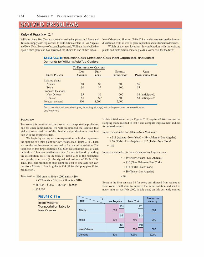
SOLVED PROBLEMSSolved Problem C.1Williams Auto Top Carriers currently maintains plants in Atlanta andTulsa to supply auto top carriers to distribution centers in Los Angelesand NewYork. Because of expanding demand, Williams has decided toopen a third plant and has narrowed the choice to one of two cities—
New Orleans and Houston. Table C.3 provides pertinent production anddistribution costs as well as plant capacities and distribution demands.
Which of the new locations, in combination with the existingplants and distribution centers, yields a lower cost for the firm?
SOLVED PROBLEMS
Solution
To answer this question, we must solve two transportation problems,one for each combination. We will recommend the location thatyields a lower total cost of distribution and production in combina-tion with the existing system.
We begin by setting up a transportation table that representsthe opening of a third plant in New Orleans (see Figure C.11). Thenwe use the northwest-corner method to find an initial solution. Thetotal cost of this first solution is $23,600. Note that the cost of eachindividual “plant-to-distribution-center” route is found by addingthe distribution costs (in the body of Table C.3) to the respectiveunit production costs (in the right-hand column of Table C.3).Thus, the total production-plus-shipping cost of one auto top car-rier from Atlanta to Los Angeles is $14 ($8 for shipping plus $6 forproduction).
Total cost = × + ×+ × + ×
= + + +=
( $ ) ( $ )( $ ) ( $ )
$ , $ , $ , $ ,
$ ,
600 14 200 9700 12 500 10
8 400 1 800 8 400 5 000
23 600
units units units units
Is this initial solution (in Figure C.11) optimal? We can use thestepping-stone method to test it and compute improvement indicesfor unused routes:
Improvement index for Atlanta–New York route
Improvement index for New Orleans–Los Angeles route
Because the firm can save $6 for every unit shipped from Atlanta toNew York, it will want to improve the initial solution and send asmany units as possible (600, in this case) on this currently unused
= +−+−
=
$
$
$
$
$
9
10
12
9
2
(New Orleans–Los Angeles)
(New Orleans–New York)
(Tulsa–New York)
(Tulsa–Los Angeles)
= + −+ −
= −
$ $$ $
$
11 149 12
6
(Atlanta–New York) (Atlanta–Los Angeles) (Tulsa–Los Angeles) (Tulsa–New York)
TABLE C.3 � Production Costs, Distribution Costs, Plant Capabilities, and MarketDemands for Williams Auto Top Carriers
TO DISTRIBUTION CENTERS
LOS NEW NORMAL UNIT
FROM PLANTS ANGELES YORK PRODUCTION PRODUCTION COST
aIndicates distribution cost (shipping, handling, storage) will be $6 per carrier between Houston and New York.
HEIZMX0C_013185755X.QXD 5/4/05 2:44 PM Page 734
IN T E R N E T A N D ST U D E N T CD-ROM EX E R C I S E S 735
FromTo
Atlanta
Tulsa
New Orleans
Demand
Los Angeles New York
800 1,200 2,000
500
900
600
800 100
$14
500
600
$9
$9
$11
$12
$10
Productioncapacity
FIGURE C.12 �
Improved TransportationTable for Williams
route (see Figure C.12). You may also want to confirm that the totalcost is now $20,000, a savings of $3,600 over the initial solution.
Next, we must test the two unused routes to see if theirimprovement indices are also negative numbers:
Index for Atlanta–Los Angeles
= $14 � $11 + $12 � $9 = $6
Index for New Orleans–Los Angeles
= $9 � $10 + $12 � $9 = $2
Because both indices are greater than zero, we have already reachedour optimal solution using the New Orleans plant. If Williams electsto open the New Orleans plant, the firm’s total production and distri-bution cost will be $20,000.
This analysis, however, provides only half the answer toWilliams’s problem. The same procedure must still be followed todetermine the minimum cost if the new plant is built in Houston.Determining this cost is left as a homework problem. You can helpprovide complete information and recommend a solution by solvingProblem C.8 (on p. 737).
Solved Problem C.2In Solved Problem C.1, we examined the Williams Auto Top Carriersproblem by using a transportation table. An alternative approach is to
structure the same decision analysis using linear programming (LP),which we explained in detail in Quantitative Module B.
Solution
Using the data in Figure C.11 (p. 734), we write the objective function and constraints as follows:
Subject to: XAtl,LA + XAtl,NY ≤ 600 (production capacity at Atlanta)
XTul,LA + XTul,NY ≤ 900 (production capacity at Tulsa)
XNO,LA + XNO,NY ≤ 500 (production capacity at New Orleans)
XAtl,LA + XTul,LA +XNO,LA ≥ 800 (Los Angeles demand constraint)
XAtl,NY + XTul,NY + XNO,NY ≥ 1200 (New York demand constraint)
INTERNET AND STUDENT CD-ROM EXERCISESINTERNET AND STUDENT CD-ROM EXERCISESVisit our Companion Web site or use your student CD-ROM to help with material in this module.
On Your Student CD-ROMOn Our Companion Web site, www.prenhall.com/heizer
• Self-Study Quizzes
• Practice Problems
• Internet Homework Problems
• Internet Cases
• PowerPoint Lecture
• Practice Problems
• Excel OM
• Excel OM Example Data Files
• POM for Windows
HEIZMX0C_013185755X.QXD 5/4/05 2:44 PM Page 735
�736 MO D U L E C TR A N S P O RTAT I O N MO D E L S
DISCUSSION QUESTIONS
1. What are the three information needs of the transportation model?2. What are the steps in the intuitive lowest-cost method?3. Identify the three “steps” in the northwest-corner rule.4. How do you know when an optimal solution has been reached?5. Which starting technique generally gives a better initial solution,
and why?6. The more sources and destinations there are for a transportation
problem, the smaller the percentage of all cells that will be used inthe optimal solution. Explain.
7. All of the transportation examples appear to apply to long dis-tances. Is it possible for the transportation model to apply on amuch smaller scale, for example, within the departments of a storeor the offices of a building? Discuss; create an example or provethe application impossible.
8. Develop a northeast-corner rule and explain how it would work.Set up an initial solution for the Arizona Plumbing problem ana-lyzed in Example C1.
9. What is meant by an unbalanced transportation problem, and howwould you balance it?
10. How many cells must all solutions use?11. Explain the significance of a negative improvement index in a
transportation-minimizing problem.12. How can the transportation method address production costs in
addition to transportation costs?13. Explain what is meant by the term degeneracy within the context
of transportation modeling.
PROBLEMS*
C.1 Find an initial solution to the following transportation problem.a) Use the northwest-corner method.b) Use the intuitive lowest-cost approach.c) What is the total cost of each method?
TO
FROM LOS ANGELES CALGARY PANAMA CITY SUPPLY
Mexico City $ 6 $18 $ 8 100
Detroit $17 $13 $19 60
Ottawa $20 $10 $24 40
Demand 50 80 70
C.2 Using the stepping-stone method, find the optimal solution to Problem C.1. Compute the total cost.
C.3 a) Use the northwest-corner method to find an initial feasible solution to the following problem. What must youdo before beginning the solution steps?
b) Use the intuitive lowest-cost approach to find an initial feasible solution. Which is better?
TO
FROM A B C SUPPLY
X $10 $18 $12 100
Y $17 $13 $ 9 50
Z $20 $18 $14 75
Demand 50 80 70
C.4 Find the optimal solution to Problem C.3 using the stepping-stone method.
C.5 Tharp Air Conditioning manufactures room air conditioners at plants in Houston, Phoenix, and Memphis.These are sent to regional distributors in Dallas, Atlanta, and Denver. The shipping costs vary, and the com-pany would like to find the least-cost way to meet the demands at each of the distribution centers. Dallas
*Note: means the problem may be solved with POM for Windows; means the problem may be solved with Excel
OM; and means the problem may be solved with POM for Windows and/or Excel OM.P
�P
�P
�P
�P
�P
HEIZMX0C_013185755X.QXD 5/4/05 2:44 PM Page 736
PRO B L E M S 737
FromTo
Demand
A
B
C
1 2 3
40
Capacity
50
30
75
1555560
10
20
30
10
30
30
45
1040
30
10
10 25
5
needs to receive 800 air conditioners per month, Atlanta needs 600, and Denver needs 200. Houston has 850air conditioners available each month, Phoenix has 650, and Memphis has 300. The shipping cost per unitfrom Houston to Dallas is $8, to Atlanta $12, and to Denver $10.The cost per unit from Phoenix to Dallas is$10, to Atlanta $14, and to Denver $9. The cost per unit from Memphis to Dallas is $11, to Atlanta $8, andto Denver $12. How many units should owner Devorah Tharp ship from each plant to each regional distrib-ution center? What is the total transportation cost? (Note that a “dummy” destination is needed to balancethe problem.)
C.6 The following table is the result of one or more iterations:
a) Complete the next iteration using the stepping-stone method.b) Calculate the “total cost” incurred if your results were to be accepted as the final solution.
C.7 The three blood banks in Franklin County are coordinated through a central office that facilitates blooddelivery to four hospitals in the region. The cost to ship a standard container of blood from each bank toeach hospital is shown in the table below. Also given are the biweekly number of containers available ateach bank and the biweekly number of containers of blood needed at each hospital. How many shipmentsshould be made biweekly from each blood bank to each hospital so that total shipment costs areminimized?
C.8 In Solved Problem C.1 (page 734), Williams Auto Top Carriers proposed opening a new plant in eitherNew Orleans or Houston. Management found that the total system cost (of production plus distribution)would be $20,000 for the New Orleans site. What would be the total cost if Williams opened a plant inHouston? At which of the two proposed locations (New Orleans or Houston) should Williams open the newfacility?
C.9 For the following Karen-Reifsteck Corp. data, find the starting solution and initial cost using the northwest-corner method. What must you do to balance this problem?
a) Find an initial solution using the northwest-corner rule. What special condition exists?b) Explain how you will proceed to solve the problem.c) What is the optimal solution?
C.12 Bell Mill Works (BMW) ships French doors to three building-supply houses from mills in Mountpelier, Nixon,and Oak Ridge. Determine the best shipment schedule for BMW from the data provided by Kelly Bell, the traf-fic manager at BMW. Use the northwest-corner starting procedure and the stepping-stone method. Refer to thefollowing table. (Note: You may face a degenerate solution in one of your iterations.)
C.13 Captain Cabell Corp. manufacturers fishing equipment. Currently, the company has a plant in Los Angeles anda plant in New Orleans. David Cabell, the firm’s owner, is deciding where to build a new plant—Philadelphiaor Seattle. Use the following table to find the total shipping costs for each potential site. Which should Cabellselect?
FromTo
Factory W
Factory Y
$3
Dress ShopA
Dress ShopB
Dress ShopC
Factoryavailability
Storedemand 30 65 135
50
50
35
$6 $7
$5
$6
Factory Z
$3
$2
$4
$8
40
Walsh Clothing Group
C.10 The Tara Tripp Clothing Group owns factories in three towns (W, Y, and Z), which distribute to three Walshretail dress shops in three other cities (A, B, and C). The following table summarizes factory availabilities, pro-jected store demands, and unit shipping costs:
�P
�P
�P
�P
HEIZMX0C_013185755X.QXD 5/4/05 2:44 PM Page 738
PRO B L E M S 739
From
Susan Helms Manufacturing Data
To
Factory 1
Factory 2
10
Warehouse1
Warehouse2
Warehouse3
Plantcapacity
Warehousedemand 1,000 2,000
2,200
2,500
2,000
7 5
6
8
Factory 3
7
8
4
9
2,000
12
Warehouse4
9
11
1,2006,700
6,200
WAREHOUSE
PLANT PITTSBURGH ST. LOUIS DENVER CAPACITY
Los Angeles $100 $75 $50 150New Orleans $ 80 $60 $90 225
Philadelphia $ 40 $50 $90 350Seattle $110 $70 $30 350
Demand 200 100 400
C.14 Susan Helms Manufacturing Co. has hired you to evaluate its shipping costs. The following table shows pre-sent demand, capacity, and freight costs between each factory and each warehouse. Find the shipping patternwith the lowest cost.
C.15 Drew Rosen Corp. is considering adding a fourth plant to its three existing facilities in Decatur, Minneapolis,and Carbondale. Both St. Louis and East St. Louis are being considered. Evaluating only the transportationcosts per unit as shown in the table, decide which site is best.
C.16 Using the data from Problem C.15 and the unit production costs in the following table, show which locationsyield the lowest cost.
LOCATION PRODUCTION COSTS ($)
Decatur $50Minneapolis 60Carbondale 70East St. Louis 40St. Louis 50
C.17 Duffy Pharmaceuticals enjoys a dominant position in the southeast U.S. with over 800 discount retail outlets.These stores are served by twice-weekly deliveries from Duffy’s 16 warehouses, which are in turn supplieddaily by 7 factories that manufacture about 70% of all of the chain’s products.
�P
�P
�P
��P
HEIZMX0C_013185755X.QXD 5/4/05 2:44 PM Page 739
740 MO D U L E C TR A N S P O RTAT I O N MO D E L S
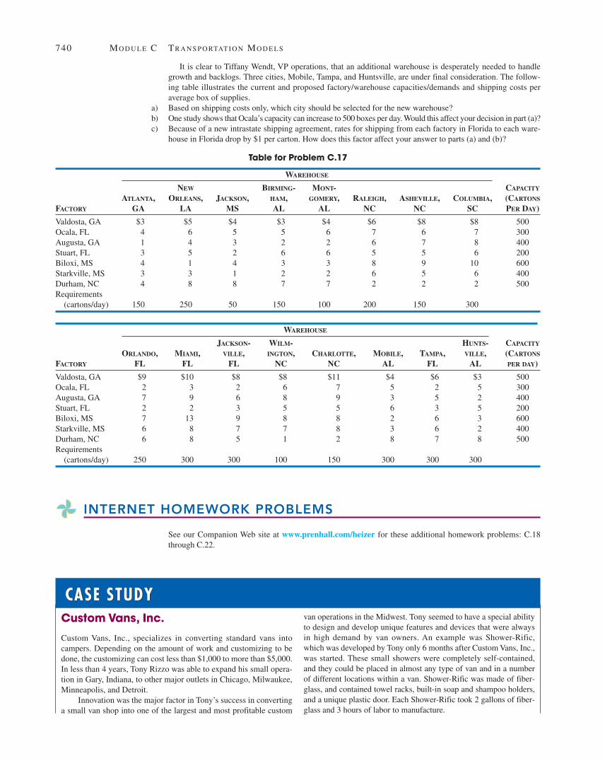
It is clear to Tiffany Wendt, VP operations, that an additional warehouse is desperately needed to handlegrowth and backlogs. Three cities, Mobile, Tampa, and Huntsville, are under final consideration. The follow-ing table illustrates the current and proposed factory/warehouse capacities/demands and shipping costs peraverage box of supplies.
a) Based on shipping costs only, which city should be selected for the new warehouse?b) One study shows that Ocala’s capacity can increase to 500 boxes per day. Would this affect your decision in part (a)?c) Because of a new intrastate shipping agreement, rates for shipping from each factory in Florida to each ware-
house in Florida drop by $1 per carton. How does this factor affect your answer to parts (a) and (b)?
Table for Problem C.17
WAREHOUSE
NEW BIRMING- MONT- CAPACITY
ATLANTA, ORLEANS, JACKSON, HAM, GOMERY, RALEIGH, ASHEVILLE, COLUMBIA, (CARTONS
See our Companion Web site at www.prenhall.com/heizer for these additional homework problems: C.18through C.22.
CASE STUDYCASE STUDYvan operations in the Midwest. Tony seemed to have a special abilityto design and develop unique features and devices that were alwaysin high demand by van owners. An example was Shower-Rific,which was developed by Tony only 6 months after Custom Vans, Inc.,was started. These small showers were completely self-contained,and they could be placed in almost any type of van and in a numberof different locations within a van. Shower-Rific was made of fiber-glass, and contained towel racks, built-in soap and shampoo holders,and a unique plastic door. Each Shower-Rific took 2 gallons of fiber-glass and 3 hours of labor to manufacture.
Custom Vans, Inc.
Custom Vans, Inc., specializes in converting standard vans intocampers. Depending on the amount of work and customizing to bedone, the customizing can cost less than $1,000 to more than $5,000.In less than 4 years, Tony Rizzo was able to expand his small opera-tion in Gary, Indiana, to other major outlets in Chicago, Milwaukee,Minneapolis, and Detroit.
Innovation was the major factor in Tony’s success in convertinga small van shop into one of the largest and most profitable custom
HEIZMX0C_013185755X.QXD 5/4/05 2:44 PM Page 740
Most of the Shower-Rifics were manufactured in Gary in thesame warehouse where Custom Vans, Inc., was founded. The manu-facturing plant in Gary could produce 300 Shower-Rifics in a month,but this capacity never seemed to be enough. Custom Van shops inall locations were complaining about not getting enough Shower-Rifics, and because Minneapolis was farther away from Gary thanthe other locations, Tony was always inclined to ship Shower-Rificsto the other locations before Minneapolis. This infuriated the man-ager of Custom Vans at Minneapolis, and after many heated discus-sions, Tony decided to start another manufacturing plant for Shower-Rifics at Fort Wayne, Indiana. The manufacturing plant at FortWayne could produce 150 Shower-Rifics per month.
The manufacturing plant at Fort Wayne was still not able tomeet current demand for Shower-Rifics, and Tony knew that thedemand for his unique camper shower would grow rapidly in thenext year. After consulting with his lawyer and banker, Tony con-cluded that he should open two new manufacturing plants as soon aspossible. Each plant would have the same capacity as the Fort Waynemanufacturing plant. An initial investigation into possible manufac-turing locations was made, and Tony decided that the two new plantsshould be located in Detroit, Michigan; Rockford, Illinois; orMadison, Wisconsin. Tony knew that selecting the best location forthe two new manufacturing plants would be difficult. Transportationcosts and demands for the various locations would be importantconsiderations.
The Chicago shop was managed by Bill Burch. This shop wasone of the first established by Tony, and it continued to outperformthe other locations. The manufacturing plant at Gary was supplying200 Shower-Rifics each month, although Bill knew that the demandfor the showers in Chicago was 300 units. The transportation cost perunit from Gary was $10, and although the transportation cost fromFort Wayne was double that amount, Bill was always pleading withTony to get an additional 50 units from the Fort Wayne manufacturer.The two additional manufacturing plants would certainly be able tosupply Bill with the additional 100 showers he needed. The trans-portation costs would, of course, vary, depending on which two loca-tions Tony picked. The transportation cost per shower would be $30from Detroit, $5 from Rockford, and $10 from Madison.
Wilma Jackson, manager of the Custom Van shop inMilwaukee, was the most upset about not getting an adequate supplyof showers. She had a demand for 100 units, and at the present time,she was only getting half of this demand from the Fort Wayne manu-facturing plant. She could not understand why Tony didn’t ship herall 100 units from Gary. The transportation cost per unit from Garywas only $20, while the transportation cost from Fort Wayne was$30. Wilma was hoping that Tony would select Madison for one ofthe manufacturing locations. She would be able to get all the showersneeded, and the transportation cost per unit would only be $5. If notin Madison, a new plant in Rockford would be able to supply hertotal needs, but the transportation cost per unit would be twice asmuch as it would be from Madison. Because the transportation costper unit from Detroit would be $40, Wilma speculated that even ifDetroit became one of the new plants, she would not be getting anyunits from Detroit.
Custom Vans, Inc., of Minneapolis was managed by Tom Poanski.He was getting 100 showers from the Gary plant. Demand was 150units. Tom faced the highest transportation costs of all locations. Thetransportation cost from Gary was $40 per unit. It would cost $10 moreif showers were sent from the Fort Wayne location. Tom was hopingthat Detroit would not be one of the new plants, as the transportationcost would be $60 per unit. Rockford and Madison would have a costof $30 and $25, respectively, to ship one shower to Minneapolis.
The Detroit shop’s position was similar to Milwaukee’s—onlygetting half of the demand each month. The 100 units that Detroit didreceive came directly from the Fort Wayne plant. The transportationcost was only $15 per unit from Fort Wayne, while it was $25 fromGary. Dick Lopez, manager of Custom Vans, Inc., of Detroit, placedthe probability of having one of the new plants in Detroit fairly high.The factory would be located across town, and the transportationcost would be only $5 per unit. He could get 150 showers from thenew plant in Detroit and the other 50 showers from Fort Wayne.Even if Detroit was not selected, the other two locations were notintolerable. Rockford had a transportation cost per unit of $35, andMadison had a transportation cost of $40.
Tony pondered the dilemma of locating the two new plants forseveral weeks before deciding to call a meeting of all the managersof the van shops. The decision was complicated, but the objectivewas clear—to minimize total costs. The meeting was held in Gary,and everyone was present except Wilma.
Tony: Thank you for coming. As you know, I have decided toopen two new plants at Rockford, Madison, or Detroit.The two locations, of course, will change our shippingpractices, and I sincerely hope that they will supply youwith the Shower-Rifics that you have been wanting. Iknow you could have sold more units, and I want you toknow that I am sorry for this situation.
Dick: Tony, I have given this situation a lot of consideration,and I feel strongly that at least one of the new plantsshould be located in Detroit. As you know, I am nowonly getting half of the showers that I need. My brother,Leon, is very interested in running the plant, and I knowhe would do a good job.
Tom: Dick, I am sure that Leon could do a good job, and I knowhow difficult it has been since the recent layoffs by theauto industry. Nevertheless, we should be considering totalcosts and not personalities. I believe that the new plantsshould be located in Madison and Rockford. I am fartheraway from the other plants than any other shop, and theselocations would significantly reduce transportation costs.
Dick: That may be true, but there are other factors. Detroit hasone of the largest suppliers of fiberglass, and I havechecked prices. A new plant in Detroit would be able topurchase fiberglass for $2 per gallon less than any of theother existing or proposed plants.
Tom: At Madison, we have an excellent labor force. This isdue primarily to the large number of students attendingthe University of Wisconsin. These students are hardworkers, and they will work for $1 less per hour than theother locations that we are considering.
Bill: Calm down, you two. It is obvious that we will not beable to satisfy everyone in locating the new plants.Therefore, I would like to suggest that we vote on thetwo best locations.
Tony: I don’t think that voting would be a good idea. Wilmawas not able to attend, and we should be looking at all ofthese factors together in some type of logical fashion.
742 MO D U L E C TR A N S P O RTAT I O N MO D E L S
BIBLIOGRAPHY
Drezner, Z. Facility Location: A Survey of Applications and Methods.Secaucus, NJ: Springer-Verlag (1995).
Haksever, C., B. Render, and R. Russell. Service Management andOperations, 2nd ed. Upper Saddle River, NJ: Prentice Hall (2000).
Koksalan, M., and H. Sural. “Efes Beverage Group Makes Locationand Distribution Decisions for Its Malt Plants.” Interfaces 29(March–April 1999): 89–103.
Ping, J., and K. F. Chu. “A Dual-Matrix Approach to theTransportation Problem.” Asia–Pacific Journal of OperationsResearch 19 (May 2002): 35–46.
Render, B., R. M. Stair, and R. Balakrishnan. Managerial DecisionModeling with Spreadsheets. 2nd. ed. Upper Saddle River, NJ:Prentice Hall (2006).
Render, B., R. M. Stair, and M. Hanna. Quantitative Analysis forManagement, 9th ed. Upper Saddle River, NJ: Prentice Hall(2006).
Schmenner, R. W. “Look Beyond the Obvious in Plant Location.”Harvard Business Review 57, 1 (January–February 1979):126–132.
Taylor, B. Introduction to Management Science, 8th ed., Upper SaddleRiver, NJ: Prentice Hall (2005).
ADDITIONAL CASE STUDIESADDITIONAL CASE STUDIES
Internet Case Studies: Visit our Companion Web site at www.prenhall.com/heizer for thesefree case studies:• Consolidated Bottling (B): This case involves determining where to add bottling capacity.
• Northwest General Hospital: This case involves minimizing the time to distribute hot food in a hospital.


![[Jay Heizer, Barry Render]Operations Management 10e](https://static.documents.pub/doc/80x56/55cf8e81550346703b92d9f3/jay-heizer-barry-renderoperations-management-10e-56427fb5ecb7b.jpg)


