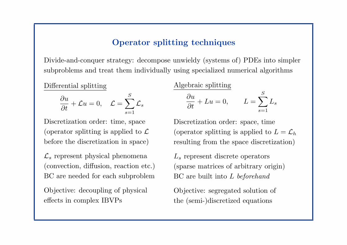
Operator splitting techniques

Divide-and-conquer strategy: decompose unwieldy (systems of) PDEs into simpler

subproblems and treat them individually using specialized numerical algorithms

Differential splitting

∂u

∂t+ Lu = 0, L =

S∑

s=1

Ls

Discretization order: time, space

(operator splitting is applied to Lbefore the discretization in space)

Ls represent physical phenomena

(convection, diffusion, reaction etc.)

BC are needed for each subproblem

Objective: decoupling of physical

effects in complex IBVPs

Algebraic splitting

∂u

∂t+ Lu = 0, L =

S∑

s=1

Ls

Discretization order: space, time

(operator splitting is applied to L = Lh

resulting from the space discretization)

Ls represent discrete operators

(sparse matrices of arbitrary origin)

BC are built into L beforehand

Objective: segregated solution of

the (semi-)discretized equations

First-order operator splitting

Initial value problem ∂u∂t + Lu = 0 in (0, T ) u(0) = u0

(Marchuk-)Yanenko method L =S∑

s=1Ls (differential or algebraic)

∂u(s)

∂t+ Lsu

(s) = 0 in (tn, tn+1) s = 1, . . . , S

u(s)(tn) = u(s−1)(tn+1), u(0)(tn+1) = un, un+1 = u(S)(tn+1)

• subproblems can be discretized independently using different methods

• the splitting error is O(∆t) so that a first-order time-stepping will do

• it is possible to treat some subproblems explicitly and some implicitly

• substepping (different time steps for different subproblems) is feasible

Remark. The decomposition of L is non-unique: L =S∑

s=1Ls =

S∑

s=1Ls

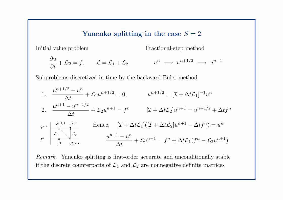
Yanenko splitting in the case S = 2

Initial value problem

∂u

∂t+ Lu = f, L = L1 + L2

Fractional-step method

un −→ un+1/2 −→ un+1

Subproblems discretized in time by the backward Euler method

1.un+1/2 − un

∆t+ L1u

n+1/2 = 0, un+1/2 = [I + ∆tL1]−1un

2.un+1 − un+1/2

∆t+ L2u

n+1 = fn [I + ∆tL2]un+1 = un+1/2 + ∆tfn

L2L1 un+1un+1=2

un+1=2tn+1tn un Hence, [I + ∆tL1]([I + ∆tL2]un+1 − ∆tfn) = un

un+1 − un

∆t+ Lun+1 = fn + ∆tL1(f

n − L2un+1)

Remark. Yanenko splitting is first-order accurate and unconditionally stable

if the discrete counterparts of L1 and L2 are nonnegative definite matrices

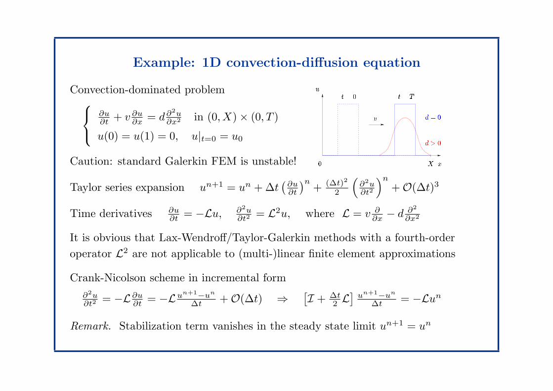
Example: 1D convection-diffusion equation

Convection-dominated problem

∂u∂t + v ∂u

∂x = d∂2u∂x2 in (0, X) × (0, T )

u(0) = u(1) = 0, u|t=0 = u0

Caution: standard Galerkin FEM is unstable!

v d = 0d > 0t = T

X x0t = 0u

Taylor series expansion un+1 = un + ∆t(

∂u∂t

)n+ (∆t)2

2

(

∂2u∂t2

)n

+ O(∆t)3

Time derivatives ∂u∂t = −Lu, ∂2u

∂t2 = L2u, where L = v ∂∂x − d ∂2

∂x2

It is obvious that Lax-Wendroff/Taylor-Galerkin methods with a fourth-order

operator L2 are not applicable to (multi-)linear finite element approximations

Crank-Nicolson scheme in incremental form

∂2u∂t2 = −L∂u

∂t = −Lun+1−un

∆t + O(∆t) ⇒[

I + ∆t2 L

]

un+1−un

∆t = −Lun

Remark. Stabilization term vanishes in the steady state limit un+1 = un

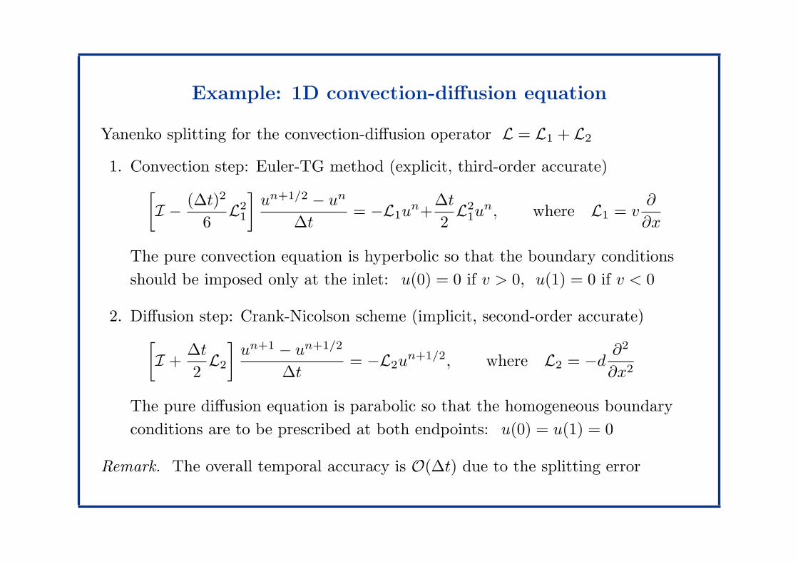
Example: 1D convection-diffusion equation

Yanenko splitting for the convection-diffusion operator L = L1 + L2

1. Convection step: Euler-TG method (explicit, third-order accurate)

[

I − (∆t)2

6L2

1

]

un+1/2 − un

∆t= −L1u

n+∆t

2L2

1un, where L1 = v

∂

∂x

The pure convection equation is hyperbolic so that the boundary conditions

should be imposed only at the inlet: u(0) = 0 if v > 0, u(1) = 0 if v < 0

2. Diffusion step: Crank-Nicolson scheme (implicit, second-order accurate)

[

I +∆t

2L2

]

un+1 − un+1/2

∆t= −L2u

n+1/2, where L2 = −d∂2

∂x2

The pure diffusion equation is parabolic so that the homogeneous boundary

conditions are to be prescribed at both endpoints: u(0) = u(1) = 0

Remark. The overall temporal accuracy is O(∆t) due to the splitting error

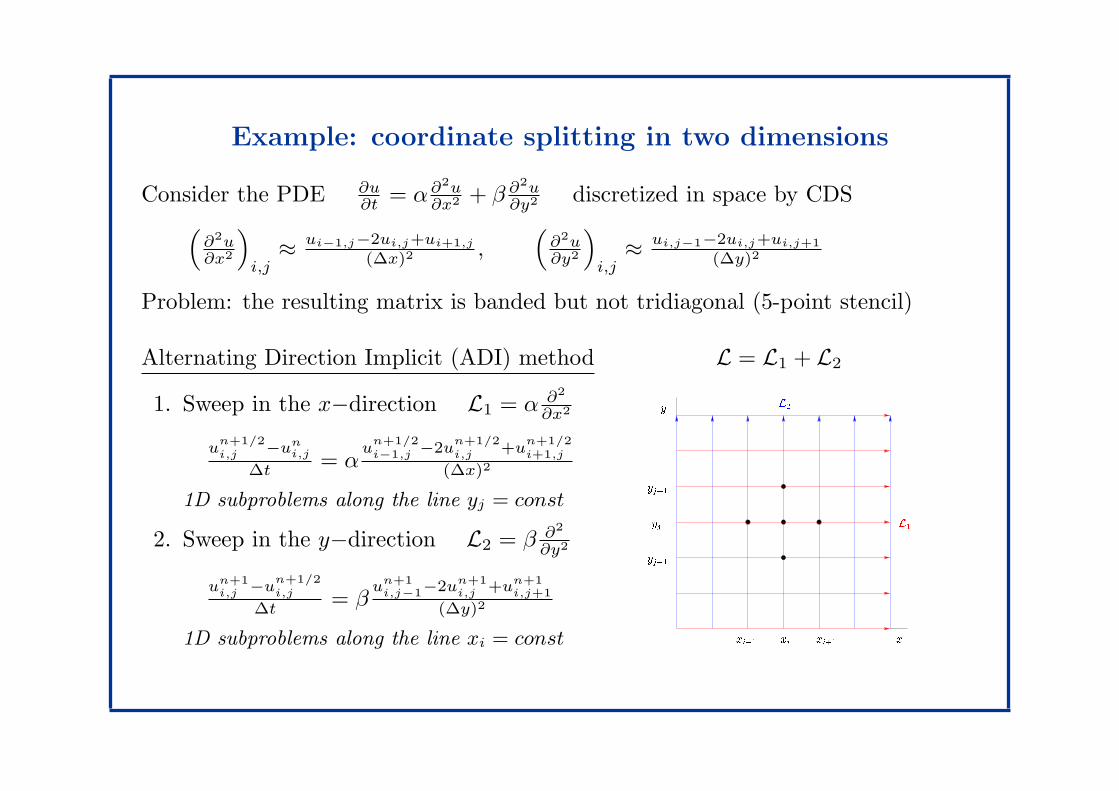
Example: coordinate splitting in two dimensions

Consider the PDE ∂u∂t = α∂2u

∂x2 + β ∂2u∂y2 discretized in space by CDS

(

∂2u∂x2

)

i,j≈ ui−1,j−2ui,j+ui+1,j

(∆x)2 ,(

∂2u∂y2

)

i,j≈ ui,j−1−2ui,j+ui,j+1

(∆y)2

Problem: the resulting matrix is banded but not tridiagonal (5-point stencil)

Alternating Direction Implicit (ADI) method L = L1 + L2

1. Sweep in the x−direction L1 = α ∂2

∂x2

un+1/2

i,j −uni,j

∆t = αu

n+1/2

i−1,j −2un+1/2

i,j +un+1/2

i+1,j

(∆x)2

1D subproblems along the line yj = const

2. Sweep in the y−direction L2 = β ∂2

∂y2

un+1

i,j −un+1/2

i,j

∆t = βun+1

i,j−1−2un+1

i,j +un+1

i,j+1

(∆y)2

1D subproblems along the line xi = consty

yj+1yj1

xi1 xi xi+1 xL2

L1yj

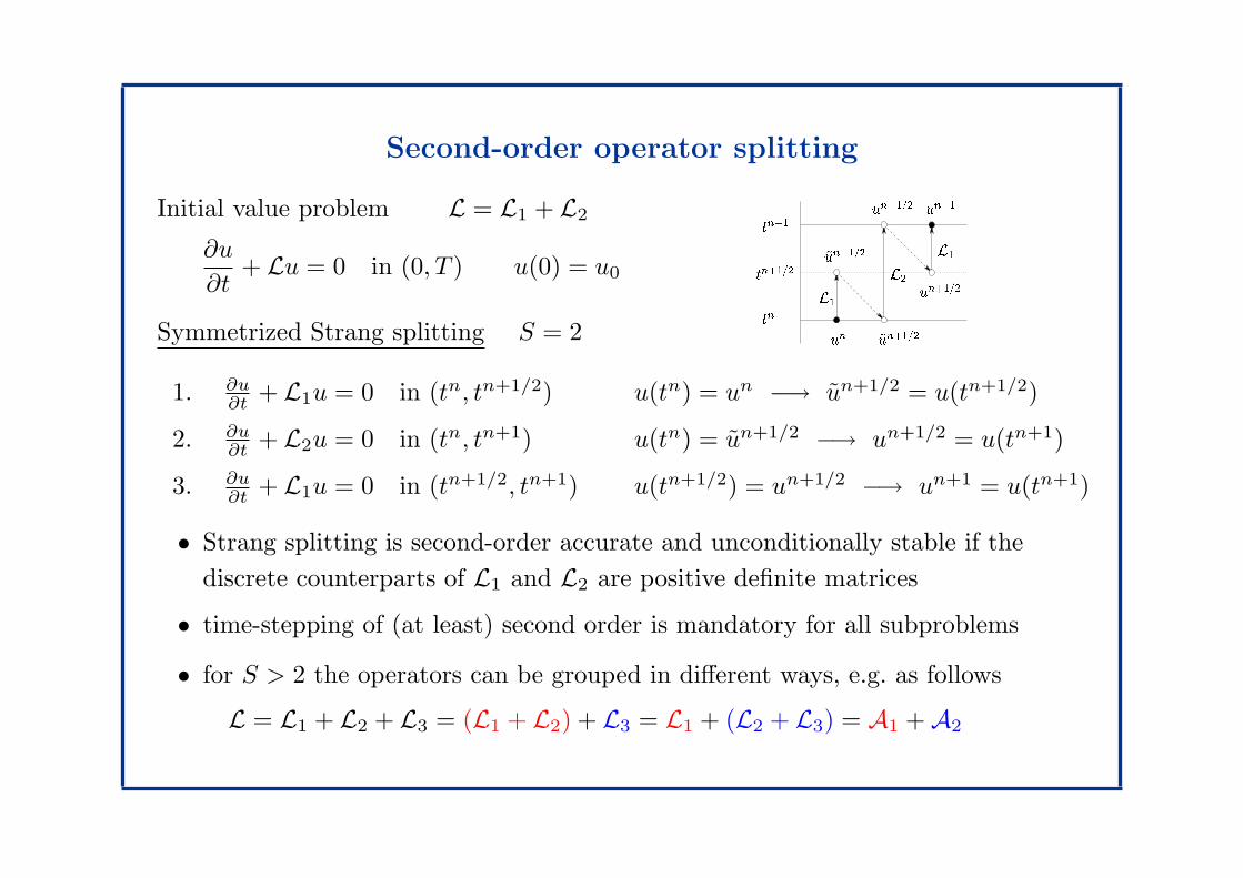
Second-order operator splitting

Initial value problem L = L1 + L2

∂u

∂t+ Lu = 0 in (0, T ) u(0) = u0

Symmetrized Strang splitting S = 2

L1L2L1 ~un+1=2tn+1=2 ~un+1=2 un+1=2un+1un+1=2tn+1

tn un

1. ∂u∂t + L1u = 0 in (tn, tn+1/2) u(tn) = un −→ un+1/2 = u(tn+1/2)

2. ∂u∂t + L2u = 0 in (tn, tn+1) u(tn) = un+1/2 −→ un+1/2 = u(tn+1)

3. ∂u∂t + L1u = 0 in (tn+1/2, tn+1) u(tn+1/2) = un+1/2 −→ un+1 = u(tn+1)

• Strang splitting is second-order accurate and unconditionally stable if the

discrete counterparts of L1 and L2 are positive definite matrices

• time-stepping of (at least) second order is mandatory for all subproblems

• for S > 2 the operators can be grouped in different ways, e.g. as follows

L = L1 + L2 + L3 = (L1 + L2) + L3 = L1 + (L2 + L3) = A1 + A2

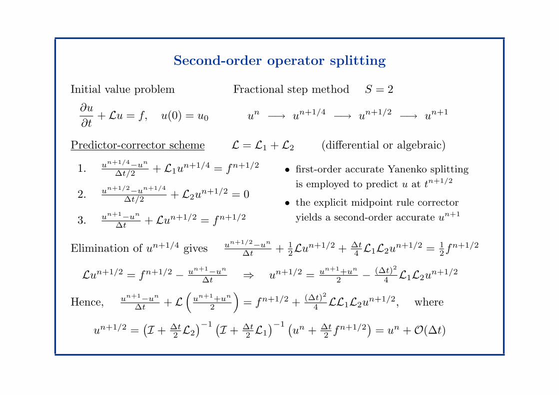
Second-order operator splitting

Initial value problem

∂u

∂t+ Lu = f, u(0) = u0

Fractional step method S = 2

un −→ un+1/4 −→ un+1/2 −→ un+1

Predictor-corrector scheme L = L1 + L2 (differential or algebraic)

1. un+1/4−un

∆t/2 + L1un+1/4 = fn+1/2

2. un+1/2−un+1/4

∆t/2 + L2un+1/2 = 0

3. un+1−un

∆t + Lun+1/2 = fn+1/2

• first-order accurate Yanenko splitting

is employed to predict u at tn+1/2

• the explicit midpoint rule corrector

yields a second-order accurate un+1

Elimination of un+1/4 gives un+1/2−un

∆t + 12Lun+1/2 + ∆t

4 L1L2un+1/2 = 1

2fn+1/2

Lun+1/2 = fn+1/2 − un+1−un

∆t ⇒ un+1/2 = un+1+un

2 − (∆t)2

4 L1L2un+1/2

Hence, un+1−un

∆t + L(

un+1+un

2

)

= fn+1/2 + (∆t)2

4 LL1L2un+1/2, where

un+1/2 =(

I + ∆t2 L2

)−1 (

I + ∆t2 L1

)−1 (

un + ∆t2 fn+1/2

)

= un + O(∆t)

Second-order operator splitting

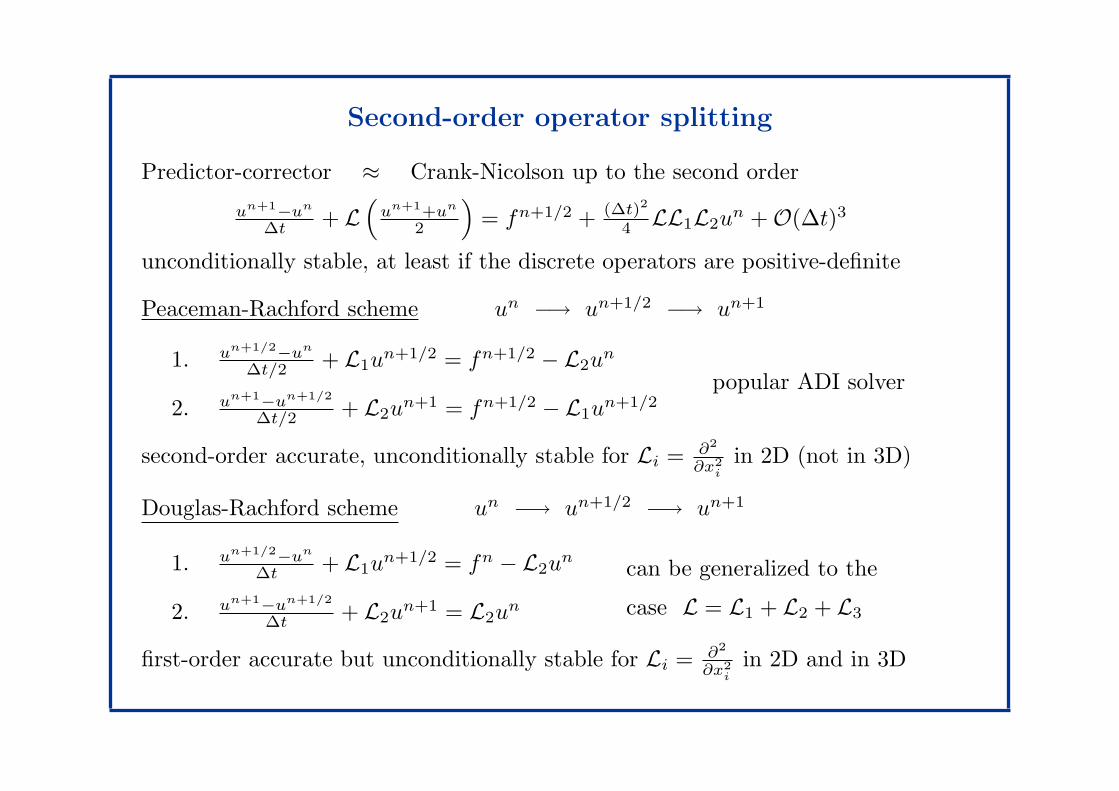
Predictor-corrector ≈ Crank-Nicolson up to the second order

un+1−un

∆t + L(

un+1+un

2

)

= fn+1/2 + (∆t)2

4 LL1L2un + O(∆t)3

unconditionally stable, at least if the discrete operators are positive-definite

Peaceman-Rachford scheme un −→ un+1/2 −→ un+1

1. un+1/2−un

∆t/2 + L1un+1/2 = fn+1/2 − L2u

n

2. un+1−un+1/2

∆t/2 + L2un+1 = fn+1/2 − L1u

n+1/2popular ADI solver

second-order accurate, unconditionally stable for Li = ∂2

∂x2i

in 2D (not in 3D)

Douglas-Rachford scheme un −→ un+1/2 −→ un+1

1. un+1/2−un

∆t + L1un+1/2 = fn − L2u

n

2. un+1−un+1/2

∆t + L2un+1 = L2u

n

can be generalized to the

case L = L1 + L2 + L3

first-order accurate but unconditionally stable for Li = ∂2

∂x2i

in 2D and in 3D

Second-order operator splitting

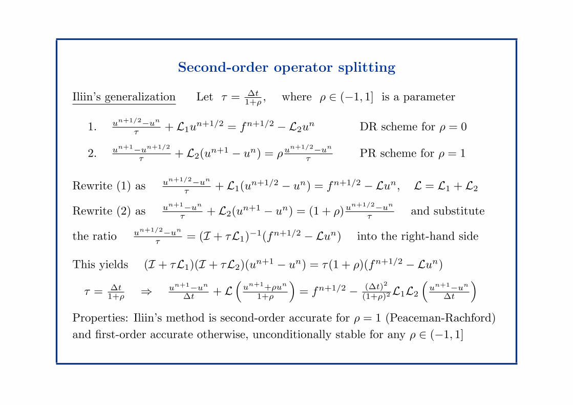
Iliin’s generalization Let τ = ∆t1+ρ , where ρ ∈ (−1, 1] is a parameter

1. un+1/2−un

τ + L1un+1/2 = fn+1/2 − L2u

n DR scheme for ρ = 0

2. un+1−un+1/2

τ + L2(un+1 − un) = ρun+1/2−un

τ PR scheme for ρ = 1

Rewrite (1) as un+1/2−un

τ + L1(un+1/2 − un) = fn+1/2 − Lun, L = L1 + L2

Rewrite (2) as un+1−un

τ + L2(un+1 − un) = (1 + ρ)un+1/2−un

τ and substitute

the ratio un+1/2−un

τ = (I + τL1)−1(fn+1/2 − Lun) into the right-hand side

This yields (I + τL1)(I + τL2)(un+1 − un) = τ(1 + ρ)(fn+1/2 − Lun)

τ = ∆t1+ρ ⇒ un+1−un

∆t + L(

un+1+ρun

1+ρ

)

= fn+1/2 − (∆t)2

(1+ρ)2L1L2

(

un+1−un

∆t

)

Properties: Iliin’s method is second-order accurate for ρ = 1 (Peaceman-Rachford)

and first-order accurate otherwise, unconditionally stable for any ρ ∈ (−1, 1]

Second-order operator splitting

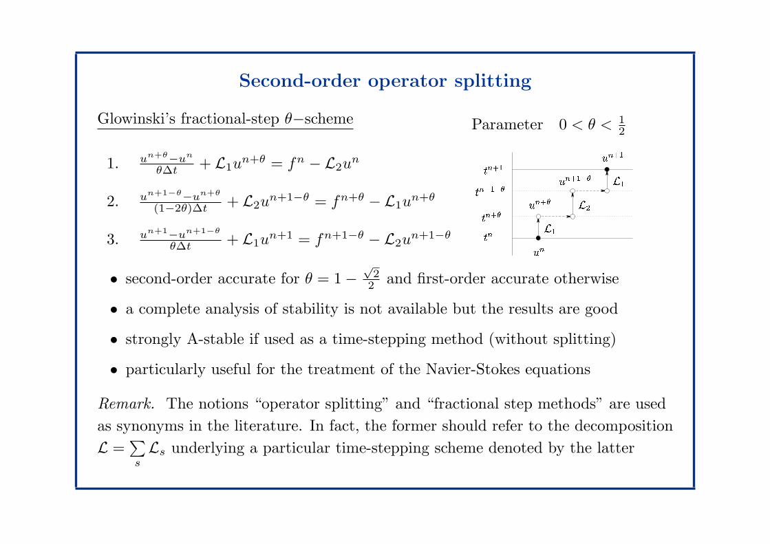
Glowinski’s fractional-step θ−scheme

1. un+θ−un

θ∆t + L1un+θ = fn − L2u

n

2. un+1−θ−un+θ

(1−2θ)∆t + L2un+1−θ = fn+θ − L1u

n+θ

3. un+1−un+1−θ

θ∆t + L1un+1 = fn+1−θ − L2u

n+1−θ

Parameter 0 < θ < 12L1L2L1tn+ un+ un+1tn+1 un+1tn+1

tn un

• second-order accurate for θ = 1 −√

22 and first-order accurate otherwise

• a complete analysis of stability is not available but the results are good

• strongly A-stable if used as a time-stepping method (without splitting)

• particularly useful for the treatment of the Navier-Stokes equations

Remark. The notions “operator splitting” and “fractional step methods” are used

as synonyms in the literature. In fact, the former should refer to the decomposition

L =∑

sLs underlying a particular time-stepping scheme denoted by the latter

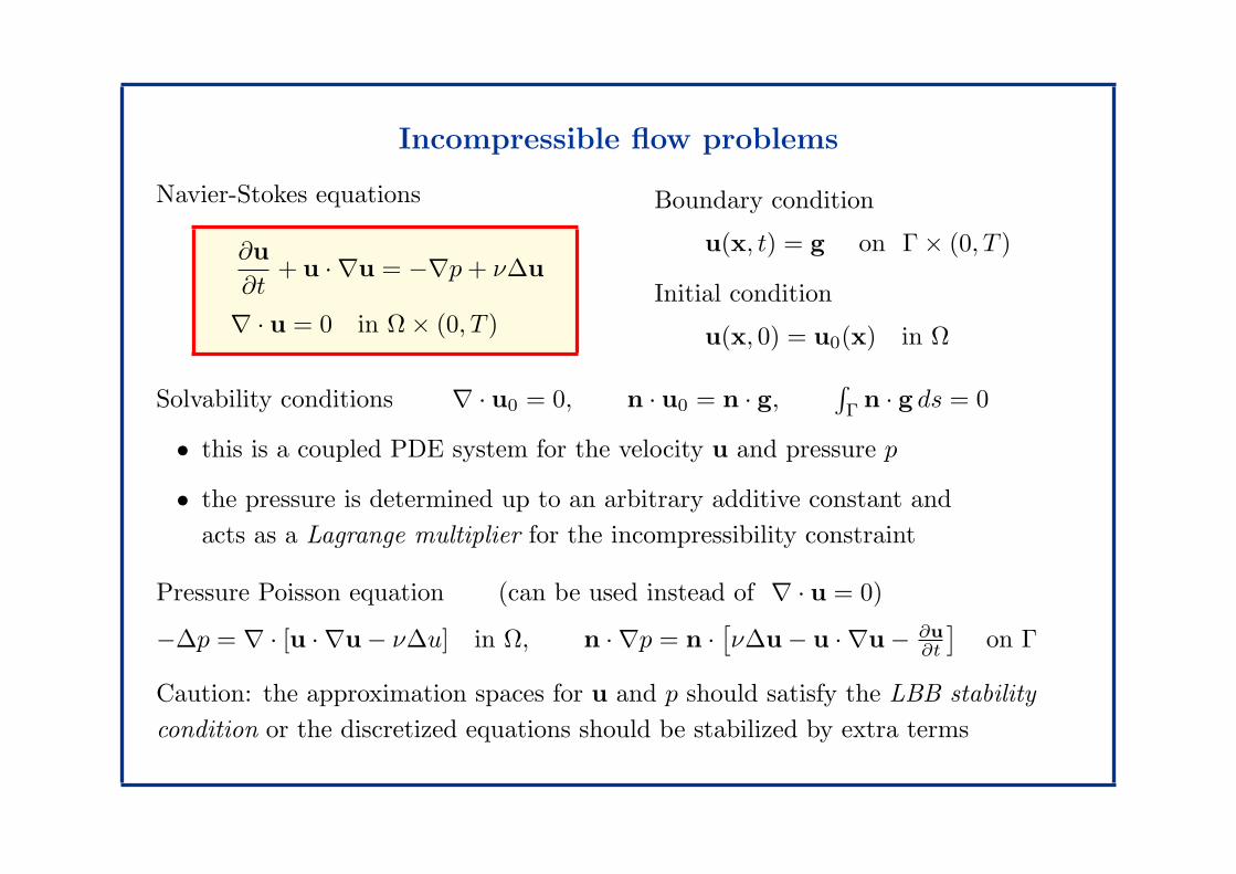
Incompressible flow problems

Navier-Stokes equations

∂u

∂t+ u · ∇u = −∇p + ν∆u

∇ · u = 0 in Ω × (0, T )

Boundary condition

u(x, t) = g on Γ × (0, T )

Initial condition

u(x, 0) = u0(x) in Ω

Solvability conditions ∇ · u0 = 0, n · u0 = n · g,∫

Γn · g ds = 0

• this is a coupled PDE system for the velocity u and pressure p

• the pressure is determined up to an arbitrary additive constant and

acts as a Lagrange multiplier for the incompressibility constraint

Pressure Poisson equation (can be used instead of ∇ · u = 0)

−∆p = ∇ · [u · ∇u − ν∆u] in Ω, n · ∇p = n ·[

ν∆u − u · ∇u − ∂u

∂t

]

on Γ

Caution: the approximation spaces for u and p should satisfy the LBB stability

condition or the discretized equations should be stabilized by extra terms

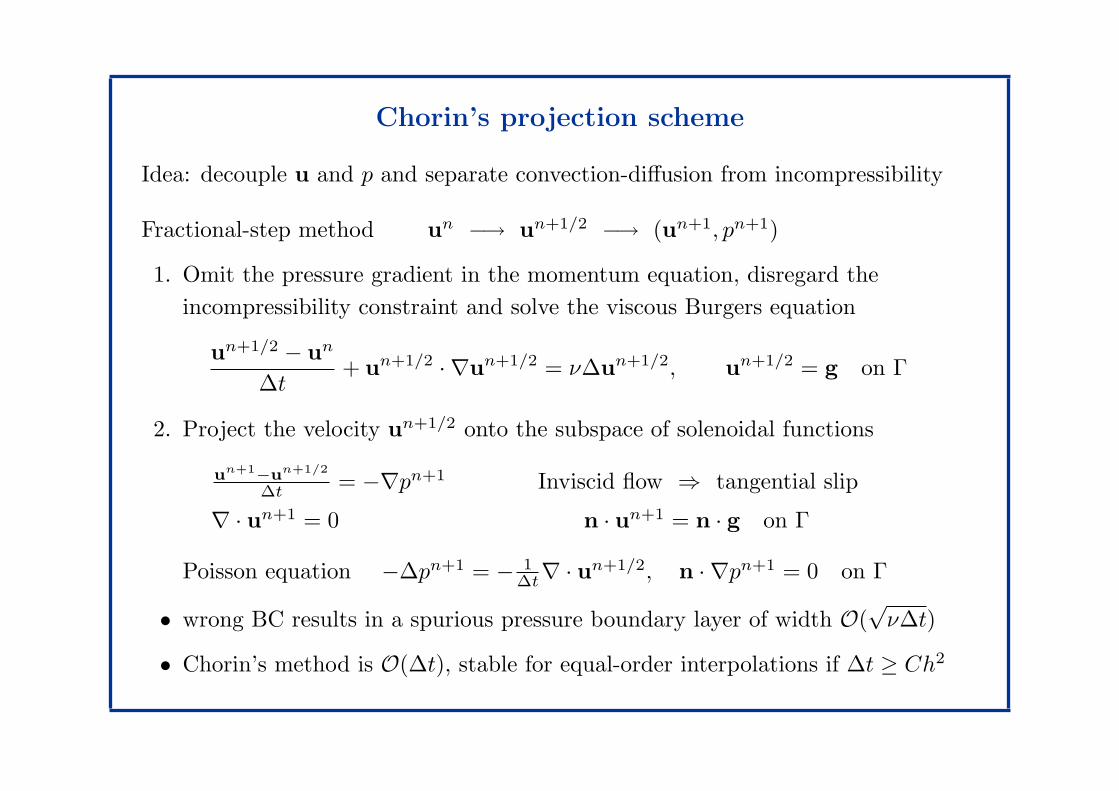
Chorin’s projection scheme

Idea: decouple u and p and separate convection-diffusion from incompressibility

Fractional-step method un −→ un+1/2 −→ (un+1, pn+1)

1. Omit the pressure gradient in the momentum equation, disregard the

incompressibility constraint and solve the viscous Burgers equation

un+1/2 − un

∆t+ un+1/2 · ∇un+1/2 = ν∆un+1/2, un+1/2 = g on Γ

2. Project the velocity un+1/2 onto the subspace of solenoidal functions

un+1−u

n+1/2

∆t = −∇pn+1 Inviscid flow ⇒ tangential slip

∇ · un+1 = 0 n · un+1 = n · g on Γ

Poisson equation −∆pn+1 = − 1∆t∇ · un+1/2, n · ∇pn+1 = 0 on Γ

• wrong BC results in a spurious pressure boundary layer of width O(√

ν∆t)

• Chorin’s method is O(∆t), stable for equal-order interpolations if ∆t ≥ Ch2

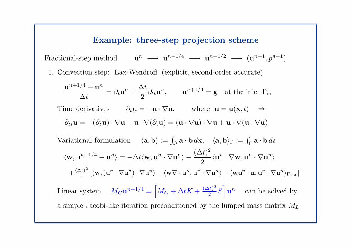
Example: three-step projection scheme

Fractional-step method un −→ un+1/4 −→ un+1/2 −→ (un+1, pn+1)

1. Convection step: Lax-Wendroff (explicit, second-order accurate)

un+1/4 − un

∆t= ∂tu

n +∆t

2∂ttu

n, un+1/4 = g at the inlet Γin

Time derivatives ∂tu = −u · ∇u, where u = u(x, t) ⇒

∂ttu = −(∂tu) · ∇u − u · ∇(∂tu) = (u · ∇u) · ∇u + u · ∇(u · ∇u)

Variational formulation 〈a,b〉 :=∫

Ωa · b dx, 〈a,b〉Γ :=

∫

Γa · b ds

〈w,un+1/4 − un〉 = −∆t〈w,un · ∇un〉 − (∆t)2

2〈un · ∇w,un · ∇un〉

+ (∆t)2

2[〈w, (un · ∇u

n) · ∇un〉 − 〈w∇ · un

,un · ∇u

n〉 − 〈wun · n,u

n · ∇un〉Γout ]

Linear system MCun+1/4 =[

MC + ∆tK + (∆t)2

2 S]

un can be solved by

a simple Jacobi-like iteration preconditioned by the lumped mass matrix ML

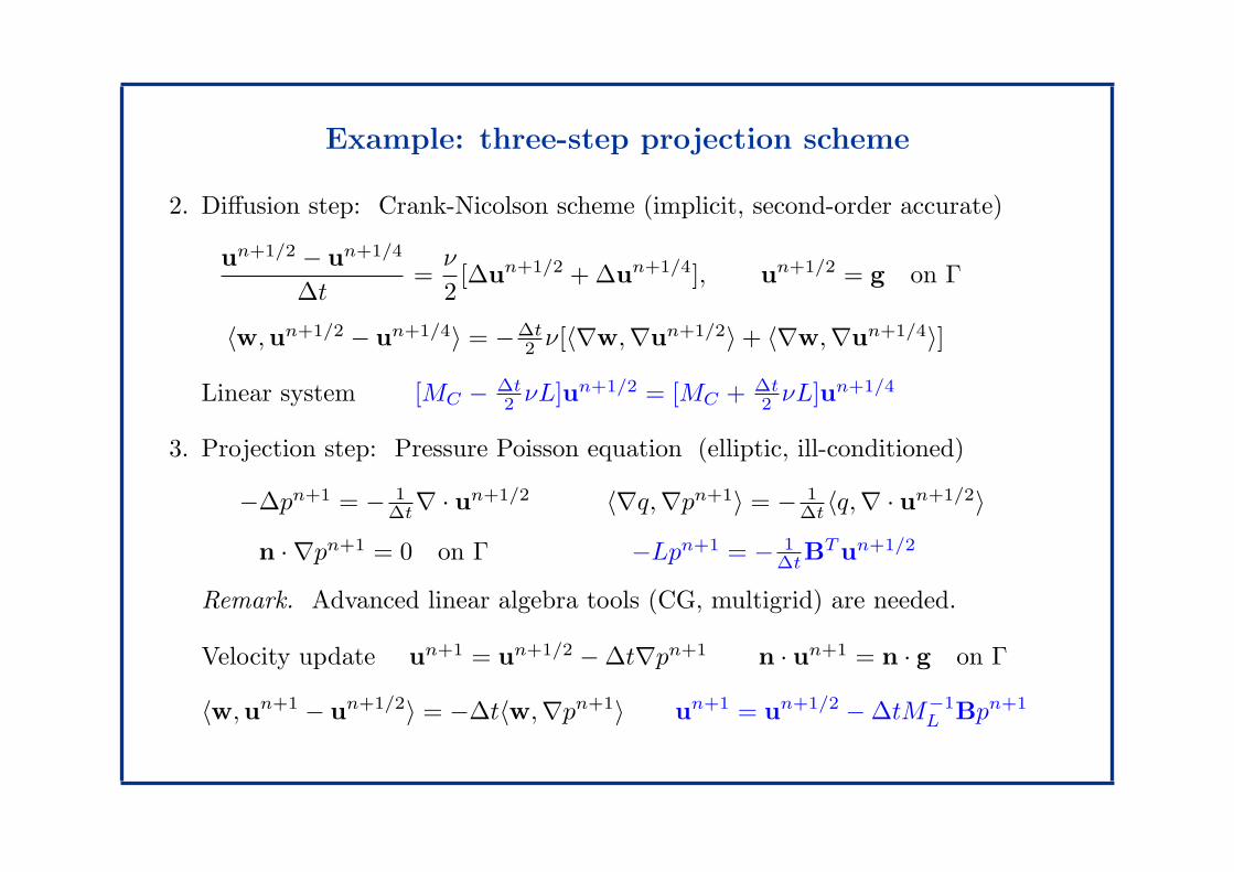
Example: three-step projection scheme

2. Diffusion step: Crank-Nicolson scheme (implicit, second-order accurate)

un+1/2 − un+1/4

∆t=

ν

2[∆un+1/2 + ∆un+1/4], un+1/2 = g on Γ

〈w,un+1/2 − un+1/4〉 = −∆t2 ν[〈∇w,∇un+1/2〉 + 〈∇w,∇un+1/4〉]

Linear system [MC − ∆t2 νL]un+1/2 = [MC + ∆t

2 νL]un+1/4

3. Projection step: Pressure Poisson equation (elliptic, ill-conditioned)

−∆pn+1 = − 1∆t∇ · un+1/2

n · ∇pn+1 = 0 on Γ

〈∇q,∇pn+1〉 = − 1∆t 〈q,∇ · un+1/2〉

−Lpn+1 = − 1∆tB

T un+1/2

Remark. Advanced linear algebra tools (CG, multigrid) are needed.

Velocity update un+1 = un+1/2 − ∆t∇pn+1 n · un+1 = n · g on Γ

〈w,un+1 − un+1/2〉 = −∆t〈w,∇pn+1〉 un+1 = un+1/2 − ∆tM−1L Bpn+1

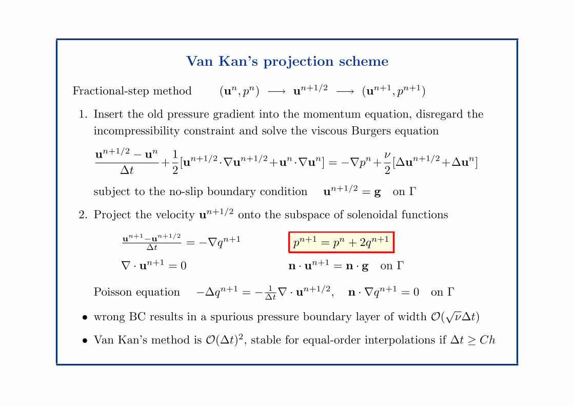
Van Kan’s projection scheme

Fractional-step method (un, pn) −→ un+1/2 −→ (un+1, pn+1)

1. Insert the old pressure gradient into the momentum equation, disregard the

incompressibility constraint and solve the viscous Burgers equation

un+1/2 − un

∆t+

1

2[un+1/2 ·∇un+1/2+un ·∇un] = −∇pn+

ν

2[∆un+1/2+∆un]

subject to the no-slip boundary condition un+1/2 = g on Γ

2. Project the velocity un+1/2 onto the subspace of solenoidal functions

un+1−u

n+1/2

∆t = −∇qn+1 pn+1 = pn + 2qn+1

∇ · un+1 = 0 n · un+1 = n · g on Γ

Poisson equation −∆qn+1 = − 1∆t∇ · un+1/2, n · ∇qn+1 = 0 on Γ

• wrong BC results in a spurious pressure boundary layer of width O(√

ν∆t)

• Van Kan’s method is O(∆t)2, stable for equal-order interpolations if ∆t ≥ Ch

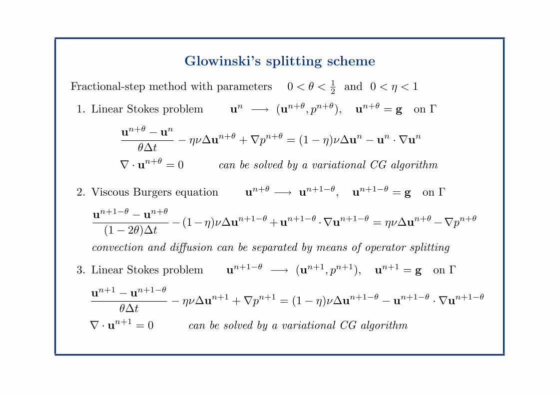
Glowinski’s splitting scheme

Fractional-step method with parameters 0 < θ < 12 and 0 < η < 1

1. Linear Stokes problem un −→ (un+θ, pn+θ), un+θ = g on Γ

un+θ − un

θ∆t− ην∆un+θ + ∇pn+θ = (1 − η)ν∆un − un · ∇un

∇ · un+θ = 0 can be solved by a variational CG algorithm

2. Viscous Burgers equation un+θ −→ un+1−θ, un+1−θ = g on Γ

un+1−θ − un+θ

(1 − 2θ)∆t− (1−η)ν∆un+1−θ +un+1−θ ·∇un+1−θ = ην∆un+θ −∇pn+θ

convection and diffusion can be separated by means of operator splitting

3. Linear Stokes problem un+1−θ −→ (un+1, pn+1), un+1 = g on Γ

un+1 − un+1−θ

θ∆t− ην∆un+1 + ∇pn+1 = (1 − η)ν∆un+1−θ − un+1−θ · ∇un+1−θ

∇ · un+1 = 0 can be solved by a variational CG algorithm

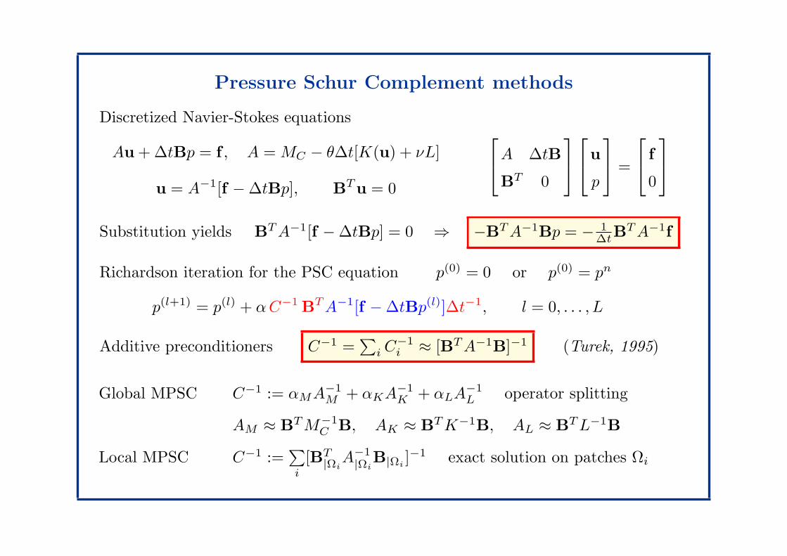
Pressure Schur Complement methods

Discretized Navier-Stokes equations

Au + ∆tBp = f , A = MC − θ∆t[K(u) + νL]

u = A−1[f − ∆tBp], BT u = 0

A ∆tB

BT 0

u

p

=

f

0

Substitution yields BT A−1[f − ∆tBp] = 0 ⇒ −BT A−1Bp = − 1∆tB

T A−1f

Richardson iteration for the PSC equation p(0) = 0 or p(0) = pn

p(l+1) = p(l) + α C−1 BT A−1[f − ∆tBp(l)]∆t−1, l = 0, . . . , L

Additive preconditioners C−1 =∑

i C−1i ≈ [BT A−1B]−1 (Turek, 1995)

Global MPSC C−1 := αMA−1M + αKA−1

K + αLA−1L operator splitting

AM ≈ BT M−1C B, AK ≈ BT K−1B, AL ≈ BT L−1B

Local MPSC C−1 :=∑

i

[BT|Ωi

A−1|Ωi

B|Ωi]−1 exact solution on patches Ωi

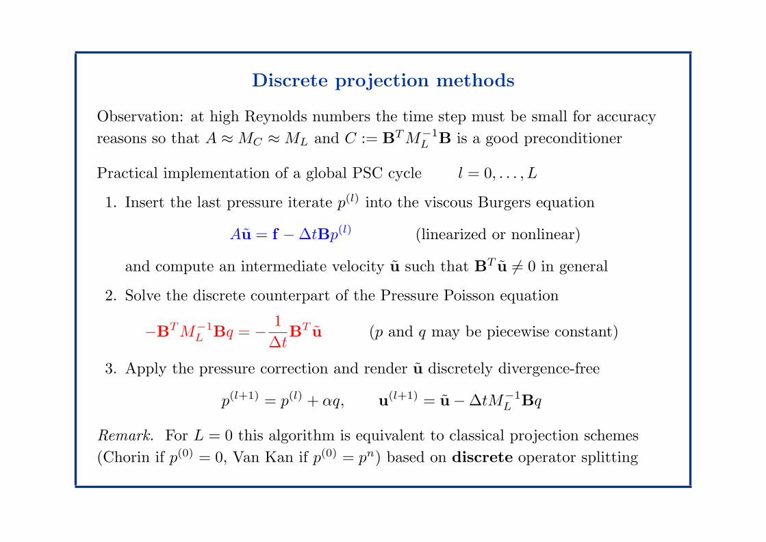
Discrete projection methods

Observation: at high Reynolds numbers the time step must be small for accuracy

reasons so that A ≈ MC ≈ ML and C := BT M−1L B is a good preconditioner

Practical implementation of a global PSC cycle l = 0, . . . , L

1. Insert the last pressure iterate p(l) into the viscous Burgers equation

Au = f − ∆tBp(l) (linearized or nonlinear)

and compute an intermediate velocity u such that BT u 6= 0 in general

2. Solve the discrete counterpart of the Pressure Poisson equation

−BT M−1L Bq = − 1

∆tBT u (p and q may be piecewise constant)

3. Apply the pressure correction and render u discretely divergence-free

p(l+1) = p(l) + αq, u(l+1) = u − ∆tM−1L Bq

Remark. For L = 0 this algorithm is equivalent to classical projection schemes

(Chorin if p(0) = 0, Van Kan if p(0) = pn) based on discrete operator splitting

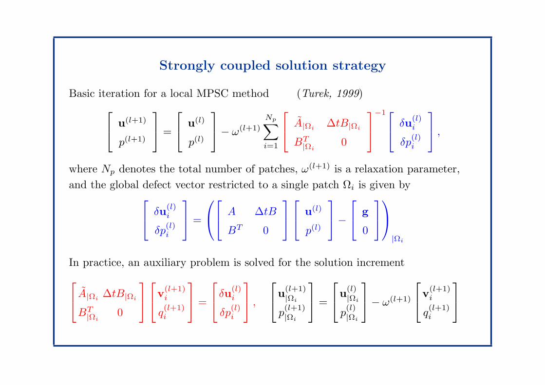
Strongly coupled solution strategy

Basic iteration for a local MPSC method (Turek, 1999)

u(l+1)

p(l+1)

=

u(l)

p(l)

− ω(l+1)

Np∑

i=1

A|Ωi∆tB|Ωi

BT|Ωi

0

−1

δu(l)i

δp(l)i

,

where Np denotes the total number of patches, ω(l+1) is a relaxation parameter,

and the global defect vector restricted to a single patch Ωi is given by

δu(l)i

δp(l)i

=

A ∆tB

BT 0

u(l)

p(l)

−

g

0

|Ωi

In practice, an auxiliary problem is solved for the solution increment

A|Ωi∆tB|Ωi

BT|Ωi

0

v(l+1)i

q(l+1)i

=

δu(l)i

δp(l)i

,

u(l+1)|Ωi

p(l+1)|Ωi

=

u(l)|Ωi

p(l)|Ωi

− ω(l+1)

v(l+1)i

q(l+1)i

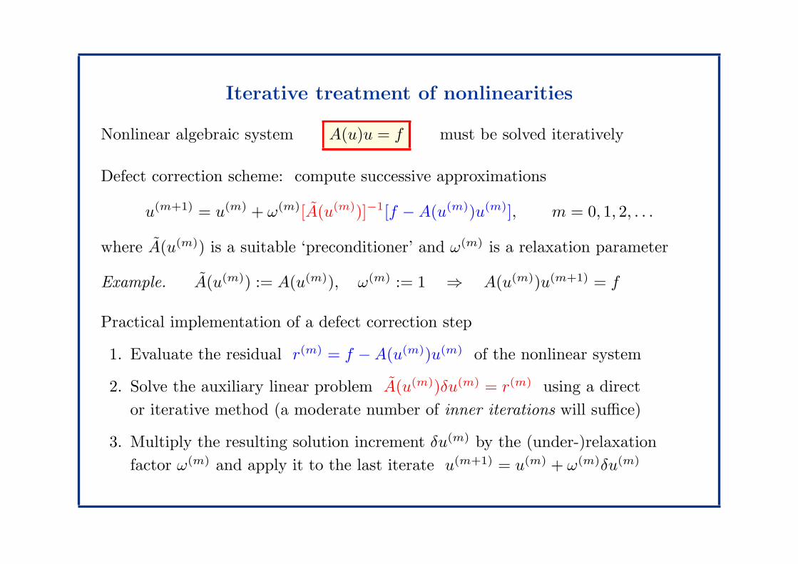
Iterative treatment of nonlinearities

Nonlinear algebraic system A(u)u = f must be solved iteratively

Defect correction scheme: compute successive approximations

u(m+1) = u(m) + ω(m)[A(u(m))]−1[f − A(u(m))u(m)], m = 0, 1, 2, . . .

where A(u(m)) is a suitable ‘preconditioner’ and ω(m) is a relaxation parameter

Example. A(u(m)) := A(u(m)), ω(m) := 1 ⇒ A(u(m))u(m+1) = f

Practical implementation of a defect correction step

1. Evaluate the residual r(m) = f − A(u(m))u(m) of the nonlinear system

2. Solve the auxiliary linear problem A(u(m))δu(m) = r(m) using a direct

or iterative method (a moderate number of inner iterations will suffice)

3. Multiply the resulting solution increment δu(m) by the (under-)relaxation

factor ω(m) and apply it to the last iterate u(m+1) = u(m) + ω(m)δu(m)